MRI channel flows and their parasites

Abstract

Local simulations of the magnetorotational instability (MRI) in accretion disks can exhibit recurrent coherent structures called channel flows. The formation and destruction of these structures may play a role in the development and saturation of MRI-induced turbulence, and consequently help us understand the time-dependent accretion behaviour of certain astrophysical objects. Previous investigations have revealed that channel solutions are attacked by various parasitic modes, foremost of which is an analogue of the Kelvin-Helmholtz instability. We revisit these instabilities and show how they relate to the classical instabilities of plasma physics, the kink and pinch modes. However, we argue that in most cases channels emerge from developed turbulence and are eventually destroyed by turbulent mixing, not by the parasites. The exceptions are the clean isolated channels which appear in systems near criticality or which emerge from low amplitude initial conditions. These structures inevitably achieve large amplitudes and are only then destroyed, giving rise to eruptive behaviour.

1 Introduction

The initiator of magnetohydrodynamic turbulence in accretion disks, and consequently of accretion itself, is most likely the magnetorotational instability (MRI) (Balbus and Hawley 1991, 1998). As its name suggests, the MRI marries differential rotation and magnetic tension which in combination draw energy from the orbital motion and direct it into rapidly growing perturbations. Numerical simulations show that the MRI excites and sustains disordered flows that transport significant angular momentum under a broad range of conditions (Hawley et al. 1995, Hawley 2000). In addition, local simulations of the MRI exhibit recurring coherent structures in which the flow vertically splits into two countermoving planar streams (Sano 2007, Lesur and Longaretti 2007). These have been termed ‘channel flows’ and coincide exactly with unstable and axisymmetric linear MRI modes (Goodman and Xu 1994). It is to these structures, their stability and role in MRI saturation, that this paper is devoted.

Goodman and Xu (1994) conducted the first analysis of the formation and breakup of channel flows. They revealed that these structures are linearly unstable to two kinds of three-dimensional parasitic mode, the fastest growing being a generalisation of the Kelvin-Helmholtz instability. However, some simulations suggest that channel destruction may in many cases be a nonlinear process involving the interaction of a number of active MRI modes; on the other hand, simulations which achieve strong magnetic fields report destabilisation by magnetic reconnection (Hawley et al. 1995, Fleming et al. 2000, Lesaffre et al. submitted). The last point highlights the potential importance of plasma microphysics in the development and saturation of the MRI, an issue that has greatly interested researchers of late (Lesaffre and Balbus 2007, Fromang et al. 2007, Pessah et al. 2007).

In this paper we investigate, with semi-analytic techniques and numerical simulations, the salient characteristics and dynamical role of channel solutions in the development of the MRI. We first revisit the study of Goodman and Xu (1994) and reinterpret their results, connecting them to work in the field of magnetic jets, while also generalising the analysis to include resistivity. Motivated by the appearance of thin intense channels in our simulations, we also generalise the analysis to include compressibility and more ‘extreme’ channel profiles. These predictions are compared to compressible three-dimensional simulations. Lastly, we argue that the mechanism of channel breakdown in most cases is inherently nonlinear, involving turbulent fluctuations, and is not a result of linear parasitic modes. We discuss briefly how this behaviour connects to the geometry of the computational domain and the plasma beta parameter $\beta$.

2 Goodman and Xu (1994) revisited

The natural starting point of our discussion is the important study of Goodman and Xu (1994), hereafter referred to as ‘GX’. This work not only revealed that certain linear MRI modes are exact nonlinear solutions, it also detailed the various instabilities to which they are subject. In this section we return to these results and clarify a few issues pertaining to the behaviour of the secondary parasitic instabilities.

In addition, we generalise the results to non-ideal MHD by introducing Ohmic resistivity. It is true in most astrophysical situations, particularly those that involve fully ionised plasmas, that resistivities are exceedingly small (though in numerical simulations they must inconveniently take larger values). But a small resistivity can have important effects in a layer encompassing the magnetic null surfaces of the channel solution: within this layer one class of parasitic mode functions similarly to the tearing mode and reconnects magnetic field.

On the other hand, we neglect viscosity, mainly for simplicity, but also because we expect its impact to be minimal on the modes in which we are interested — lowering their growth rates and slightly restricting instability to longer wavelengths. Viscosity will also alter the MRI channel structure itself, but this is only appreciable when the Reynolds number is extremely small, less than about 10 (Pessah and Chan 2008), much smaller than in astrophysical systems and simulations. Recently, research has explored the connection between the magnetic Prandtl number and the saturation of MRI induced turbulence (Fromang et al. 2007, Lesur and Longaretti 2007). We do not believe, however, that this connection extends to parasitic modes as well, nor their dependence on viscosity. More likely, the magnetic Prandtl number dependence issues from the separation of the two dissipative scales, the viscous and resistive, and how this impacts on the turbulent cascade of energy (Balbus and Hawley 1998, Balbus and Henri 2008).

Before we plunge into the analysis we must first set up the problem, exhibit the governing equations, and provide a little background to the MRI itself. This is undertaken in the following section.

2.1 Governing equations

We study a disk of conducting fluid orbitting a massive compact object. Its motion is described by the orbital frequency $\Omega(r)$ (a function of cylindrical radius $r$) and it is threaded by vertical magnetic field $\mathbf{B}=B_{0}\,\mathbf{e}_{z}$. Initially we assume the imposed magnetic field is weak and the Alfvén speed much less than the sound speed. Typical fluid velocities are also assumed much less than the sound speed because fluid motion is (at first) triggered by magnetic tension. As a consequence, we adopt the equations of incompressible nonideal MHD.

The equations are framed in the geometry of the shearing sheet, which is a standard local approximation that describes a small ‘block’ of disk centred at a radius $r_{0}$ moving on the circular orbit $r_{0}$ prescribes. The model provides an adequate approximation to phenomena that vary on length-scales much less than the large-scale properties of the disk. The block is represented in Cartesian coordinates with the $x$ and $y$ directions corresponding to the radial and azimuthal directions respectively. To account for the differential rotation we add a Coriolis force and impose a background linear shear, $\mathbf{v}=2A_{0}\,x\,\mathbf{e}_{y}$, where

$$A_{0}=\frac{r_{0}}{2}\left(\frac{d\Omega}{dr}\right)_{0}.$$

A Keplerian disk yields $A_{0}=-3/4$. Though we leave $A_{0}$ free in the following, we nearly always let it take its Keplerian value for applications.

The governing equations are

$$\frac{\partial\mathbf{v}}{\partial t}+\mathbf{v}\cdot\nabla\mathbf{v}=-\frac{1}{\rho_{0}}\nabla\left(P+\frac{B^{2}}{8\pi}\right)+\frac{\mathbf{B}\cdot\nabla\mathbf{B}}{4\pi\rho_{0}}$$

$$\hskip 113.81102pt-2\mathbf{\Omega}\times\mathbf{v}-4A_{0}\Omega_{0}\,x\,\mathbf{e}_{x},$$ (1)

$$\frac{\partial\mathbf{B}}{\partial t}=\nabla\times(\mathbf{v}\times\mathbf{B})+\eta\nabla^{2}\mathbf{B},$$ (2)

$$\nabla\cdot\mathbf{B}=0,$$ (3)

$$\nabla\cdot\mathbf{v}=0$$ (4)

where $\mathbf{\Omega}=\Omega_{0}\mathbf{e}_{z}$, and $\Omega_{0}=\Omega(r_{0})$. The resistivity is denoted by $\eta$ and $\rho_{0}$ is the homogeneous background mass density, a constant. To this set we must add appropriate boundary conditions. For convenience, the ‘0’ subscripts on $A_{0}$ and $\Omega_{0}$ will be dropped.

By construction, the governing equations admit the equilibrium solution of linear shear and uniform vertical field: $\mathbf{v}=2\,A\,x\,\mathbf{e}_{y}$ and $\mathbf{B}=B_{0}\,\mathbf{e}_{z}$. But this configuration, as has been well established, is violently unstable to the MRI for a sufficiently weak imposed $\mathbf{B}$ (Balbus and Hawley 1991). Small perturbations of the form $e^{st+iKz}$ grow rapidly and exhibit growth rates of order an orbital period. The most vigorous mode grows at a rate $s=-A$.

The instability gives rise to a vertical sequence of planar countermoving fluid streams, or channels. What is remarkable is that this configuration not only corresponds to the linear eigenfunction of the MRI but to a nonsteady but exact nonlinear solution to the set Eqs (1)-(4) (GX). As a consequence, in our discussion on channels it will be as an exact nonlinear solution that we treat the MRI, not as a Fourier-decomposed linear mode. In the next section it is described mathematically.

2.2 MRI channels

We adhere to the approach of GX, differing only in the introduction of resistivity. Our ansatz for the MRI channel solution is

$$\mathbf{v}^{\text{ch}}=b\,e^{st}\,v_{0}\,\sin(Kz)\,(\mathbf{e}_{x}\cos\theta+\mathbf{e}_{y}\sin\theta)$$ (5)

$$\mathbf{B}^{\text{ch}}=b\,e^{st}\,B_{0}\,\cos(Kz)\,(\mathbf{e}_{x}\cos\phi+\mathbf{e}_{y}\sin\phi)$$ (6)

where $s$ is the growth rate of the mode, $K$ is its vertical wavenumber, $b$ is a dimensionless measure of the channel amplitude, and $v_{0}$ and $B_{0}$ are dimensional constants. Note that there exist two orientation angles $\theta$ and $\phi$; if resistivity were absent we would only require one, because the $\mathbf{B}$ field is then perpendicular to $\mathbf{v}$ (i.e. $\phi=\theta-\pi/2$).

These functions are superimposed on the background linear shear and vertical field, so that

$$\mathbf{v}=\mathbf{v}^{\text{ch}}+2A\,x\,\mathbf{e}_{y},\qquad\mathbf{B}=\mathbf{B}^{\text{ch}}+B_{0}\,\mathbf{e}_{z},$$

and then substituted into the $x$ and $y$ components of the governing equations (1) and (2). Because $\mathbf{v}^{\text{ch}}\cdot\nabla\mathbf{v}^{\text{ch}}=\mathbf{B}^{\text{ch}}\cdot\nabla\mathbf{B}^{\text{ch}}=0$ and $\mathbf{v}^{\text{ch}}\cdot\nabla\mathbf{B}^{\text{ch}}=\mathbf{B}^{\text{ch}}\cdot\nabla\mathbf{v}^{\text{ch}}=0$ the nonlinear equations coincide with their linearised counterparts, and the solution is straightforward. It yields the dimensionless growth rate $s/\Omega$, the scaled flow speed $v_{0}K/\Omega$, the scaled channel wavenumber $v_{A}K/\Omega$, and the orientation of the magnetic field $\phi$, as functions of the dimensionless inputs $A/\Omega$, $\theta$, and $R_{m}$, where the Alfvén velocity and magnetic Reynolds number are defined through

$$v_{A}\equiv\frac{B_{0}}{\sqrt{4\pi\rho_{0}}},\qquad\qquad R_{m}\equiv\frac{\Omega}{\eta K^{2}}.$$

After a little algebra one finds

$$s =-A\,\sin 2\theta-\frac{\Omega}{R_{m}}\,\left(1+\frac{A}{\Omega}\,\cos^{2}\theta\right),$$ (7)

$$\left(v_{A}K\right)^{2} =-4\,\Omega\,A\,\sin^{2}\theta\left(1+\frac{A}{\Omega}\,\cos^{2}\theta\right)\left(1+\tfrac{1}{2}R_{m}^{-1}\,\cot\theta\right)^{2},$$ (8)

$$v_{0} =-2\frac{A}{K}\,\sin^{2}\theta\left(1+\tfrac{1}{2}R_{m}^{-1}\cot\theta\right)^{2}\,\left(1+\tfrac{1}{4}R_{m}^{-2}\right)^{-1/2},$$ (9)

$$\phi =\left(\theta-\frac{\pi}{2}\right)+\cot^{-1}\left(2R_{m}\right),$$ (10)

In the limit of $R_{m}\to\infty$ the GX ideal MHD expressions are recovered, cf. their Eqs (5)-(7). A large $R_{m}$ introduces a small correction of $1/R_{m}$ to these expressions.

The dispersion relation is a quartic in $s$ and can be computed by eliminating $\theta$ from equations (7) and (8). It is

$$(s\tilde{s}+v_{A}^{2}K^{2})^{2}+4\Omega(\Omega+A)\tilde{s}^{2}+4A\Omega v_{A}^{2}K^{2}=0,$$

with $\tilde{s}=s+\eta K^{2}$. This agrees with a number of examples in the literature; for instance, see Sano and Miyama (1999), Fleming et al.  (2000), Lesur and Longaretti (2007), or Pessah and Chan (2008). The most vigorously growing channel takes an orientation of

$$\theta_{\text{max}}=\frac{\pi}{4}+\frac{1}{2}\,\cot^{-1}(2R_{m})$$

and exhibits the growth rate

$$s_{\text{max}}=-A\sqrt{1+\tfrac{1}{4}R_{m}^{-2}}-\frac{1}{2R_{m}}(2\Omega+A).$$

At leading order in large $R_{m}$ we recover $\theta=\pi/4$ and $s_{\text{max}}=-A$, as expected.

Equation (8) tells us that $(v_{A}K)^{2}$ is a decreasing function of $\theta$. Therefore, longer wavelength MRI modes possess flows that are more radial and magnetic fields that are more toroidal. In fact, $\theta\to 0$ as $K$ approaches 0 (the marginal stability limit of very long modes). In contrast, $\theta$ approaches a value near $\pi/2$ as $K$ approaches $K_{c}$ (the marginal stability limit of short modes). Thus short wavelength MRI modes near criticality possess flows nearly azimuthal and magnetic fields nearly radial.

The Alfvénic Mach number is defined by $M_{A}\equiv v_{0}/v_{A}$, and can be computed from (8) and (9). We find that the strongest growing channels are characterised by fluid speeds comparable and less than the Alfvén velocity, $M_{A}\lesssim 1$. This is because the acceleration which drives the flow issues from magnetic tension. Generally, sub-Alfvénic flows are stable to shear instabilities because of the (relatively) large magnetic tension (Chandrasekhar 1961). That being so, shear instabilities in MRI channel flows may orient themselves perpendicular to $\mathbf{B}^{\text{ch}}$ and escape this constraint. Happily for them, $\mathbf{B}^{\text{ch}}$ and $\mathbf{v}^{\text{ch}}$ are nearly perpendicular, and it is this fortuitous orientation that allows so much scope for the parasitic instabilities that afflict channel solutions.

Finally, from Eq. (10) it is clear that decreasing $R_{m}$ also decreases the opening angle between the magnetic and velocity fields. The effect, however, is rather small until $R_{m}\lesssim 10$. In most ionised plasma the angle should be virtually 90 degrees; but in the interiors of protostellar disks it may be somewhat less.

Being a nonlinear solution, a channel mode will retain its structure and grow exponentially regardless of its amplitude. Unperturbed it will continue to do so until the approximation of incompressiblity fails. This will happen when the Alfvén speed, and the speed of the fluid jets, approach the sound speed of the fluid itself. At this point in the evolution, layers of magnetic field either side of a channel will give rise to a magnetic pressure ‘sink’ sufficiently strong to squeeze mass towards the magnetic null surfaces at $Kz=(2n+1)\,\pi/2$ (for $n=0,1,\dots$). These altitudes are also where the fluid jets are maximal. As a consequence, the channel structure will evolve from the sinusoidal profiles of (5) and (6) towards a more ‘extreme’ configuration. In fact, if undisturbed, we may end up with a sequence of discontinuous current sheets concentrating nearly all the mass and all the velocity upon the magnetic null surfaces. Such sheets were briefly analysed by GX who rightly exhibited them as the opposite (compressible) limit to the incompressible MRI channels (see Fig. 13 later for a numerical approximation).

In any case, if an incompressible MRI channel is to reach the amplitudes at which compressibility plays a role, the channel must grow undisrupted for a significant amount of time. One could be forgiven for thinking that this may not be all that frequent an occurrence. On one hand, early in its growth, an MRI channel may interact with a different competing MRI mode, and this interaction could lead to the early disruption of both. On the other hand, parasitic instabilities may emerge upon the channel structure feeding off its energy and ultimately leading to its demise. For the remainder of this section we examine the latter possibility; in so doing we rediscuss the analysis of GX and connect it to relevant work in the field of magnetohydrodynamical jets and magnetic reconnection. Once this is finished we suggest that, in fact, the large amplitude regime is more likely than one might think.

2.3 Parasitic modes

The linear stability of nonlinear channel solutions is complicated for a number of reasons, not least by the fact that the channels are time-dependent: they grow exponentially. This means we are not strictly permitted to deploy the familiar techniques of linear analysis. In particular, small perturbations cannot be, in general, Fourier-decomposed in time. Modal solutions of the type $e^{\sigma t}$ exist only when the growth rate $\sigma$ is much larger than the growth rate $s$ of the channel solution itself, because then, as far as the mode is concerned, the background is steady (GX). This is the case when the amplitudes of the channels are large, as a consequence of the scaling $\sigma\sim b\Omega$. So when $b\gg 1$, it follows that $\sigma\gg\Omega\sim s$.

In order to make progress, we assume the limit of large channel amplitude and search for parasitic modes of type $\propto e^{\sigma t}$. The task then simplifies, requiring the solution of a boundary value problem in one variable with eigenvalue $\sigma$.

2.3.1 Linearised equations

The channel solutions outlined in the previous section are perturbed by a small disturbance so that

$$\mathbf{v}=2Ax\,\mathbf{e}_{y}+\mathbf{v}^{\text{ch}}+\mathbf{v}^{\prime},\quad\mathbf{B}=B_{0}\,\mathbf{e}_{z}+\mathbf{B}^{\text{ch}}+\mathbf{B}^{\prime},\quad P=P_{0}+P^{\prime},$$

where the prime denotes the small perturbation. These are subtituted into Eqs (1), (2), and (4) which are linearised in the perturbations. The next step is to assume that the channel amplitudes are large, i.e. $b\gg 1$, and that the time dependence of the perturbation scales as $\partial_{t}\sim b\Omega$. This renders the background shear, Coriolis force, uniform vertical field, and the exponential growth of the channel solution all negligible. The channel structure is hence reduced to a stationary equilibrium and so (within the assumptions made) we are permitted to search for Fourier modes of the type $\mathbf{v}^{\prime},\mathbf{B}^{\prime},P^{\prime}\propto e^{\sigma t+ik_{x}x+ik_{y}y}$. The analysis reduces to an 8th order boundary value problem in $z$ with eigenvalue $\sigma$. Its details are now sketched out.

Units are chosen so that $K=1$ and $b\Omega=1$. The velocity, magnetic, and pressure perturbations are scaled by $bv_{0}$, $bB_{0}$, and $bv_{0}^{2}$ respectively. The linearised equations read as

$$\sigma\,\mathbf{v}^{\prime} =-V\left\{\,v_{z}^{\prime}\,\partial_{z}\mathbf{v}^{0}+i(\mathbf{k}\cdot\mathbf{v}^{0})\,\mathbf{v}^{\prime}+(i\mathbf{k}+\mathbf{e}_{z}\,\partial_{z})\Psi^{\prime}\,\right\}$$

$$\hskip 49.79231pt+\frac{V}{M_{A}^{2}}\left\{B_{z}^{\prime}\,\partial_{z}\mathbf{B}^{0}+i(\mathbf{k}\cdot\mathbf{B}^{0})\,\mathbf{B}^{\prime}\right\},$$ (11)

$$\sigma\,\mathbf{B}^{\prime} =V\left\{\,B_{z}^{\prime}\,\partial_{z}\mathbf{v}^{0}-u_{z}^{\prime}\,\partial_{z}\mathbf{B}^{0}\right.$$

$$\left.+\,i(\mathbf{k}\cdot\mathbf{B}^{0})\,\mathbf{v}^{\prime}-i(\mathbf{k}\cdot\mathbf{v}^{0})\,\mathbf{B}^{\prime}\,\right\}-\frac{1}{bR_{m}}(k^{2}-\partial_{z}^{2})\mathbf{B}^{\prime}$$ (12)

$$0 =i\mathbf{k}\cdot\mathbf{v}^{\prime}+\partial_{z}v_{z}^{\prime},$$ (13)

where the total pressure is

$$\Psi^{\prime}=P^{\prime}+\frac{|B^{\prime}|^{2}}{8\pi\rho_{0}},$$

the scaled channel velocity is $V=v_{0}K/\Omega$, which can be computed from Eq. (9), the planar wavenumber is defined by $\mathbf{k}=(k_{x},k_{y},0)$, and $M_{A}$ is the Alfvénic Mach number. Finally, the background equilibrium fields are given by

$$\mathbf{v}^{0}=\sin z\,(\mathbf{e}_{x}\,\cos\theta+\mathbf{e}_{y}\,\sin\theta),$$

$$\mathbf{B}^{0}=\cos z\,(\mathbf{e}_{x}\,\cos\phi+\mathbf{e}_{y}\,\sin\phi).$$

The linear operator associated with this problem is $2\pi$-periodic in $z$, and we thus make the Floquet ansatz:

$$\mathbf{v}^{\prime}=\widetilde{\mathbf{v}}(z)\,e^{ik_{z}z},\qquad\mathbf{B}^{\prime}=\widetilde{\mathbf{B}}(z)\,e^{ik_{z}z},\qquad\Psi^{\prime}=\widetilde{\Psi}(z)\,e^{ik_{z}z},$$

where the functions $\widetilde{\mathbf{v}}(z)$, $\widetilde{\mathbf{B}}(z)$, $\widetilde{\Psi}(z)$ are $2\pi$-periodic in $z$. The Floquet exponent $k_{z}$ denotes the wavenumber of the perturbations’ vertical ‘envelope’, i.e. the large-scale structure greater than the channel width. The envelope wavenumber $k_{z}$ takes values between $0$ and $0.5$. If $k_{z}$ extends beyond this range then we repeat, or ‘alias’, eigensolutions which appear when $0<k_{z}<0.5$. The Floquet decomposition reduces the problem to the domain $[0,2\pi]$, one channel wavelength, and furnishes us with the appropriate boundary conditions: the tilde eigenfunctions must be periodic.

Now the problem is fully determined. Given the parameters $A/\Omega$, $\theta$, $R_{m}$, and $b$, on one hand, and $k_{x}$, $k_{y}$, and $k_{z}$ on the other we can compute the eigenfunctions of the parasites and their growth rates $\sigma$. Usually, we replace $k_{x}$ and $k_{y}$ with the planar wavenumber magnitude $k=\sqrt{k_{x}^{2}+k_{y}^{2}}$ and orientation angle $\theta_{k}=\arctan(k_{y}/k_{x})$. Also, for most occasions $\theta=\pi/4$ which corresponds to the fastest growing channel in ideal MHD. Other orientations were tried but we observed no change in the qualitative features of the results. A more meaningful parameter, therefore, may be $(\theta-\theta_{k})$ rather than $\theta_{k}$ itself. This angle difference measures the relative orientation of the mode’s wavevector to the fluid flow, and hence the degree to which it can extract shear energy, on one hand, and the degree to which it escapes magnetic tension, on the other.

In GX, the linearised equations could be worked into a neat second order ODE by shifting to Lagrangian variables. Unfortunately, the resistive term prevents us from attempting a similar trick: the magnetic field is no longer frozen into the fluid and as a consequence the induction equation cannot be immediately integrated. Instead, we solve the set of equations numerically via a pseudospectral technique. The $z$-domain is partitioned into $N$ grid points and the operator (2.3.1)-(13) discretised, with the derivatives computed using Fourier cardinal functions (see Boyd 2000). A $7N\times 7N$ matrix equation ensues taking the form of a generalised algebraic eigenvalue problem; this yields a spectrum that approximates that of the original differential operator. The eigenvalues $\sigma$ are obtained using standard linear algebra routines (the QZ algorithm, inverse iteration, etc). In the next few subsections we present the results: in the ideal MHD case, and with finite $R_{m}$. But first, we discuss the interpretation of the parasitic modes.

2.3.2 Mode identification

In GX two classes of parasitic mode were shown to assail a developed MRI channel solution. They were named Type 1 and Type 2 modes. The first was identified as the familiar Kelvin-Helmholtz instability, but the nature of the second was a little more difficult to assess. In fact, the Type 2 mode can be understood in the context of MHD jets as something of a hybrid mode, consisting of motions associated with both the kink and pinch modes (Drazin and Reid 1981, Biskamp 2000). In this subsection we sketch out this idea.

In the fluids literature the classic jet profile takes the form $\text{sech}^{2}(z)$, the so-called ‘Bickley jet’ (Bickley 1937), though other jet profiles offer the same qualitative behaviour (Drazin and Reid 1981). The Bickley jet is susceptible to two classes of growing mode that have picked up a variety of names: there are the ‘kink’ (or ‘odd’, ‘Kelvin-Helmholtz’, ‘sinuous’) modes, and the ‘pinch’ (or ‘even’, ‘sausage’, ‘varicose’) modes. The names arise because the former buckles (or kinks) the jet vertically, while the other squeezes and expands adjacent regions into a pattern akin to a sausage. Quite generally, the kink mode grows faster than the pinch mode. But when a parallel magnetic field is present the kink mode can be suppressed by magnetic tension which resists the mode’s attempt to bend the jet and its embedded magnetic field lines (Chandrasekhar 1961). On the other hand, the pinch mode can tap into the free energy locked up in the magnetic configuration, to some extent, and enhance its growth (Biskamp et al. 1998, Biskamp 2000). If field lines are permitted to break and reconnect (i.e. if $R_{m}$ is finite) further energy is available to the pinch mode and it adopts some of the characteristics of a tearing mode.

The Type 1 and Type 2 parasitic modes of the MRI channel problem are the generalisations of the kink and pinch modes to a situation comprising an infinite periodic lattice of countermoving jets. As such, they are global modes, attacking all the channels concurrently and are hence able to exhibit structure larger than one channel width. This larger scale structure is summarised by the Floquet factor $e^{ik_{z}z}$. In comparison, the classical pinch and kink modes are local modes which attack an isolated channel. (In real accretion disks, this ‘global structure’ — and the structure of the channel itself — will be influenced by the disk’s vertical stratification and boundary conditions.) The Type 1 mode we interpret as the straightforward generalisation of the kink mode; it is a stationary instability and buckles both sets of inward and outward jets concurrently. The Type 2 mode is a little more complicated. We interpret it as a hybrid kink and pinch mode: each Type 2 mode ‘kinks’ one set of jets (either the inward or the outward sets) while ‘pinching’ the other set of jets. There are hence two Type 2 modes and their growth rates are complex conjugates, meaning they manifest as travelling waves. We sometimes refer to the Type 2 mode as ‘the kink-pinch mode’.

The key parameter which distinguishes between the two types of parasite is the Floquet exponent, $k_{z}$. The generalised kink mode is characterised by small $k_{z}$ and the pinch mode by larger $k_{z}$. The transition between the two, as $k_{z}$ is varied, is rapid but smooth.

2.3.3 Ideal MHD

We begin by reexamining the ideal MHD case, setting the resistive terms to zero. The problem now returns to that tackled by GX; we briefly restate some of their results.

First, we exhibit the analytic stability criteria derived by GX which are derived in the long horizontal wavelength limit. Because these long modes are the most susceptible to instability they give conditions on stability generally. When $k_{z}=0$, which corresponds to a classic Type 1 instability, or ‘kink’ mode, stability is assured if

$$|\theta-\theta_{k}|>\arctan M_{A}.$$ (14)

Note that the Alfvénic Mach number is a complicated function of $\theta$ but is always $\lesssim 1$. Therefore, a very rough, but revealing, estimate of stability is $|\theta-\theta_{k}|>\pi/4$. For the $k_{z}=0$ kink mode to grow, its wavevector must be sufficiently aligned with the jet velocity, within some angle less than 45 degrees. The more the wavevector $\mathbf{k}$ points away from $\mathbf{v}^{\text{ch}}$, the less shear energy is available and the greater the magnetic tension. Two-stream channels appear regularly in numerical studies and in such simulations only $k_{z}=0$ kink parasites can fit into the computational domain. Thus the criterion (14) is the key one to keep in mind.

In contrast, when $k_{z}$ is non zero (a parameter choice associated with some Type 1 kink modes and all the Type 2 modes) the stability criterion is more stringent: these modes grow more easily. We have stability when

$$|\theta-\theta_{k}|>\arctan(M_{A}/3),$$ (15)

from which the rough estimate $|\theta-\theta_{k}|>\pi/3$ can be derived as above. Such modes grow for a wider range of orientations. Somehow the global structure, absent in the $k_{z}=0$ case, allows them to better resist magnetic tension.

The two types of mode discovered by GX can be distinguished by the parameter $k_{z}$. If $k$ and $\theta_{k}$ are fixed and we vary $k_{z}$ from $0$ to $0.5$, the mode transforms smoothly (though not uniformly) from the Type 1 kink mode to the Type 2 kink-pinch mode. When $0\leq k_{z}\lesssim 0.2$ we obtain kink modes, and when $0.2\lesssim k_{z}\leq 0.5$ we obtain kink-pinch modes. The actual values, however, depend somewhat on $k$ and in a complicated fashion, so we omit these details. We also omit the graphs of the growth rates as functions of $k$, as these appear in GX. In summary, Type 1 modes grow at a rate an order of magnitude larger than Type 2 modes with the maximum rate at values near $k=1/2$. Neither class of mode can grow when $k\geq 1$.

In the following four figures we plot representative examples of the two classes of mode. We set $\mathbf{k}$ and $\mathbf{v}^{\text{ch}}$ parallel to each other, by enforcing $\theta_{k}=\theta=\pi/4$. At this orientation both kink and pinch modes enjoy the greatest access to the shear energy of the background flow. At the same time, they are completely free of magnetic tension, being perpendicular to $\mathbf{B}^{\text{ch}}$. Consequently, these modes are virtually hydrodynamic, consigning their magnetic perturbations to the total pressure.

Fig. 1 shows three components of the kink mode eigenfunction, for which $k_{z}=0$. Note that the total pressure perturbation $\widetilde{\Psi}$ changes sign at the two altitudes $z=\pi/2$ and $3\pi/2$, which are where the two magnetic null surfaces are located, and to where the fluid jets are concentrated. Hence a pressure gradient exists across each jet and this gives rise to a buckling, or kink, motion. This motion can be observed in the $\widetilde{u}_{z}$ perturbation, which possesses maxima and minima at the jet centres: the jets are deflected upward or downward. To emphasise this point, we present in Fig. 2 the real part of the $x$ component of $\mathbf{v}^{\text{ch}}+\mathbf{v}^{\prime}$ in the $(x,z)$ plane. The background is a four-stream channel and we show two periods (in $x$) of the velocity. The kinking of the four inward and the four outward jets is pronounced, as is the formation of nascent Kelvin-Helmholtz type billows.

Fig. 3 shows three components of the Type 2 mode for the same parameters save $k_{z}$, which takes the value $0.5$. If we turn our attention first to the altitude $z=3\pi/2$ we notice that the eigenfunction behaves similarly to the kink mode: the total pressure perturbation changes sign at the centre of the jet and $\widetilde{u}_{z}$ possesses a maximum there. However, the companion jet at altitude $z=\pi/2$ undergoes a different kind of perturbation. Here it is the $\widetilde{u}_{z}$ perturbation which changes sign; accordingly, fluid above and below the jet will be either attracted to the centre of the jet or repelled. This is characteristic of the pinch, or sausage, motion. In Fig. 4 the $x$-component of the perturbed four-stream channel velocity is presented, as before, in which we can observe the alternate kinking and pinching of neighbouring jets. There exists a companion Type 2 mode with complex conjugate growth rate, and its eigenfunction reverses the kink and pinch motions to $z=\pi/2$ and $3\pi/2$ respectively.

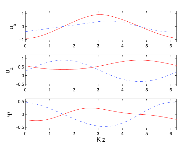
Figure 1: The $\widetilde{u}_{x}$, $\widetilde{u}_{z}$, and $\widetilde{\Psi}$ components of the eigenfunction of the kink mode with $\theta=\theta_{k}=\pi/4$ and $k/K=0.5$ and $k_{z}=0$. The solid line represents the real part and the dashed line represents the imaginary part. Note that the pressure pertubation $\widetilde{\Psi}$ changes sign at $Kz=\pi/2$ and $3\pi/2$ which are the altitudes at which the two jets are concentrated. A kinking or buckling of the jet is the outcome. Because $\theta=\theta_{k}$ the mode is effectively hydrodynamic. The total eigenfunction is normalised so that $\text{max}|\tilde{u}_{x}|=1$. The growth rate is $\sigma/(b\Omega)=0.1959$.

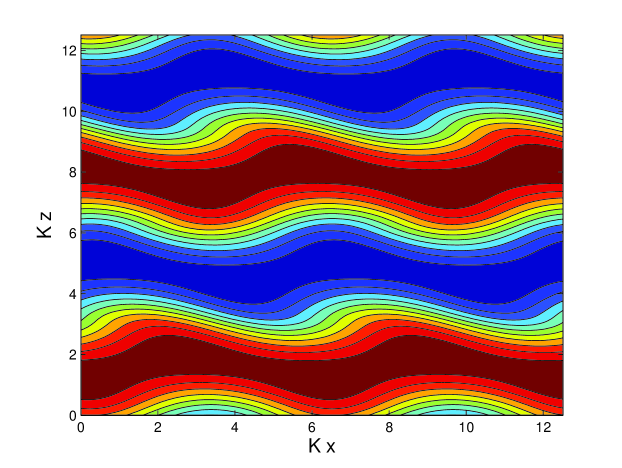
Figure 2: Coloured iso-contours of the real part of $v^{\text{ch}}_{x}+v_{x}^{\prime}$ at $y=0$ for the kink mode in the $(x,z)$ plane. Parameters chosen are $\theta=\theta_{k}=\pi/4$, $k_{x}/K=0.5$, and $k_{z}=0$. The background is a four-stream MRI channel with jets centred at $Kz=n\pi/2$ with $n=1$, $3$, $5$, and $7$. The perturbation is normalised so that $\text{max}|u_{x}^{\prime}|$ is a a quarter of $\mathbf{v}^{\text{ch}}$.

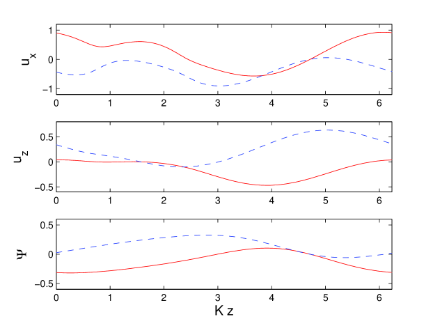
Figure 3: The $\widetilde{u}_{x}$, $\widetilde{u}_{z}$, and $\widetilde{\Psi}$ components of the eigenfunction of the kink-pinch mode with $\theta=\theta_{k}=\pi/4$ and $k/K=0.5$ and $k_{z}/K=0.5$. Note that the pressure perturbation $\widetilde{\Psi}$ changes sign at $Kz=3\pi/2$, giving rise to a kinking motion upon the jet centred there, while the vertical velocity perturbation $\widetilde{u}_{z}$ changes sign at $Kz=\pi/2$ giving rise to a pinching motion upon the jet centred there. Because $\theta=\theta_{k}$ the mode is effectively hydrodynamic. The growth rate is $\sigma/(b\Omega)=0.0931-0.1319\,i$.

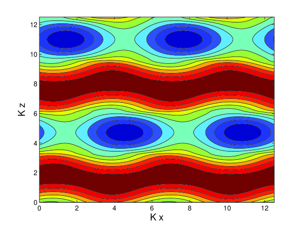
Figure 4: Coloured iso-contours of the real part of $v^{\text{ch}}_{x}+v_{x}^{\prime}$ at $y=0$ for the kink-pinch mode in the $(x,z)$ plane. Parameters chosen are $\theta=\theta_{k}=\pi/4$, $k_{x}/K=0.5$, and $k_{z}/K=0.5$. The background is a four-stream MRI channel with jets centred as before. Note the alternate kinking and pinching of the jets. Also the entire pattern is moving to the right because $\sigma$ possesses a negative imaginary component.

Next we examine the eigenmodes for different wavevector orientations. In particular, we examine axisymmetric modes, $\theta_{k}=0$, when $\theta=\pi/4$. At this configuration only modes with nonzero $k_{z}$ grow (Eq. (14)), and we limit ourselves to $k_{z}=0.5$. In these cases the background magnetic field plays a larger role in the dynamics, and leads to smaller growth rates and more stable short scales. In Figs 5 and 6 we present six components of the eigenfunction when $k=0.25$. In Fig. 5 the $\widetilde{u}_{z}$ and $\widetilde{\Psi}$ perturbations are similar to their ‘hydrodynamical’ $\theta_{k}=\theta$ cousins in Fig. 3. Note however the extra structure exhibited by the $\widetilde{u}_{x}$ component near $z=\pi/2$, $\pi$ and $2\pi$. These abrupt variations react to the contortions of the $\widetilde{B}_{x}$ and $\widetilde{B}_{y}$ magnetic perturbations frozen into the fluid. But at the pinch altitude $z=\pi/2$, the magnetic perturbations are precisely zero; this means that the pinch motion here preserves the magnetic null surface of the background channel flow. Here the channel’s magnetic field lines are symmetrically squeezed towards the null surface, or symmetrically repelled. In contrast, at the kink altitude $z=3\pi/2$, the null surface is distorted upward or downward alongside the field lines.

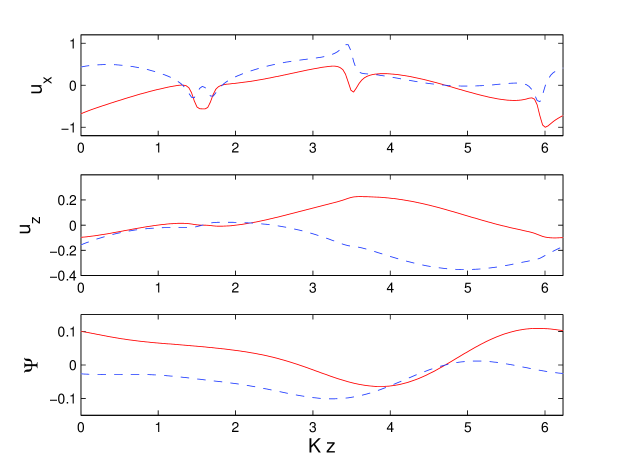
Figure 5: The $\widetilde{u}_{x}$, $\widetilde{u}_{z}$, and $\widetilde{\Psi}$ components of the eigenfunction of the kink-pinch mode when $\theta=\pi/4$ and $\theta_{k}=0$ with $k/K=0.25$ and $k_{z}/K=0.5$. Resistivity is set to zero. The mode is hence axisymmetric and magnetic stresses play an important part in the dynamics. The pinch motion is located at $Kz=\pi/2$ and the kink at $Kz=3\pi/2$. The growth rate is $\sigma/(b\Omega)=0.0142-0.1216\,i$.

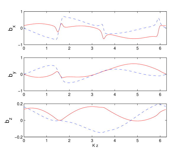
Figure 6: The magnetic components of the eigenfunction of the kink-pinch mode of Fig. 5 when $\theta=\pi/4$ and $\theta_{k}=0$ with $k/K=0.25$ and $k_{z}/K=0.5$. Note that at the pinch at $Kz=\pi/2$ the components are all zero and thus the magnetic null surface of the channel solution is preserved.

GX suspected that the pinch motion associated with the Type 2 mode would lead to reconnection at the null surface when resistivity is present, and to the consequent formation of magnetic islands, or plasmoids. Such behaviour has been seen in isolated jets by Wang et al. (1988) and Biskamp et al. (1998). We investigate this phenomenon in the next subsection in the case of a periodic lattice of MRI channels.

2.3.4 Resistive MHD

The magnetic Reynolds number $R_{m}$ is now set to finite values and the channel amplitude $b$ enters as another parameter. A number of changes take place: (a) the structure and growth rate of the kink-pinch mode alters, and (b) new growing ‘pure-pinch’, or ‘pinch-tearing’, modes emerge. Meanwhile, the kink mode’s structure and growth rate do not change significantly, nor those modes that possess wavevectors perpendicular to $\mathbf{B}^{\text{ch}}$.

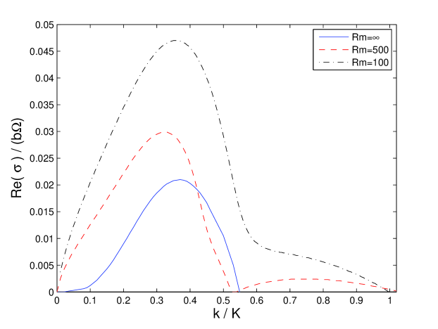
Figure 7: The real part of the growth rate $\sigma$ as a function of $k$ for an axisymmetric Type 2 mode ($\theta_{k}=0$) when $\theta=\pi/4$ and $k_{z}/K=0.5$ in the resistive and ideal cases. The solid curve corresponds to the ideal $R_{m}=\infty$ case, the dashed line to the $R_{m}=500$ and $b=5$ case, and the dotted-dashed line to the $R_{m}=100$ and $b=5$ case. Note the larger growth rates and the extended range of instability when resistivity is present. Note also that for intermediate $R_{m}$ there is a range of $k$ for which resistivity plays a ‘diffusive’ damping role. Also be aware that changing $R_{m}$ also alters the underlying equilibria slightly in each case.

The resistive Type 2 modes achieve growth rates larger than their ideal MHD counterparts, an increase which seems to scale like $(bR_{m}/M_{A})^{-3/5}$ (in agreement with studies of the tearing mode, cf. White 1986). By removing the constraint of flux conservation, the mode can reconnect magnetic field where it pinches the field lines. It thus gains access to extra energy stored in the channel’s magnetic configuration. Such energy is additional to that extracted from the velocity shear and allows the mode to grow more rapidly. These increases can be observed in Fig. 7 for an axisymmetric pinch mode with $b=5$ and $R_{m}=\infty$, $500$, and $100$. Resistivity also transforms the long wavelength behaviour of the mode: its growth rate no longer scales as $k^{3}$ for small $k$; instead, $\sigma$ possesses a much steeper dependence on $k$ (some fractional power). Conversely, instability emerges on shorter scales previously forbidden by ideal MHD: the ‘second hump’ in Fig. 7. Similar short-scale behaviour has been reported by Biskamp et al. (1998) for an isolated two-dimensional jet but with $\mathbf{B}^{\text{ch}}$ parallel to $\mathbf{v}^{\text{ch}}$.

The $R_{m}=500$ curve reflects more complicated behaviour at intermediate $R_{m}$ and deserves a few extra comments. On a small band of $k$ near $0.5$ the ideal MHD mode grows faster than the resistive mode; in addition the large and small $k$ branches of $\sigma$ detach. Note that resistivity alters the background equilibria, so the two modes are not exactly analogous. But even if this is taken into account, the resistive growth rates remain slightly lower for these values of $k$. We conclude that resistivity’s ‘diffusive role’ is anomalously important on this narrow range of intermediate scales and counteracts the extra growth stimulated by reconnection. When resistivity is sufficiently strong ($R_{m}\lesssim 250$) the effect vanishes.

The eigenfunction of the resistive kink-pinch mode does not differ significantly from its ideal MHD counterpart. The most notable distinction is in the magnetic perturbations which no longer preserve the magnetic null surface at the pinch altitude (cf. Fig. 6). Instead, a chain of magnetic islands are formed. (In the interest of brevity these profiles are not presented.)

Resistivity stimulates the growth of new ‘pure-pinch’ or ‘pinch-tearing’ modes. These extract little to no energy from the velocity shear their growth relying solely on the reconnection of magnetic field. Consequently, they favour wavevector orientations along or near $\mathbf{B}^{\text{ch}}$ and do not grow at all when $\mathbf{k}$ is perpendicular to the magnetic field. Typically the growth rates are small with $\sigma\sim 0.01$, though they can appear for all $k_{z}$ (unlike the kink and kink-pinch modes).

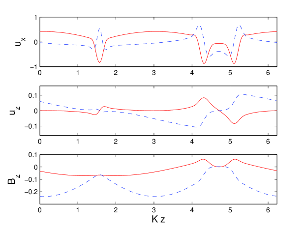
Figure 8: Selected eigenfunction profile for a general pinch-tearing mode. Parameters are $\theta=\pi/4$, $\theta_{k}=-\pi/6$, $k_{z}=0$ and $k/K=0.4$, while $R_{m}=500$ and $b=5$. The growth rate is $\sigma/(b\Omega)=0.0096$. Though the mode pinches both jets concurrently it localises preferentially on the upper one. A companion mode, growing at the same rate, localises on the lower jet.

Their fastest growth is achieved, naturally, when $\theta_{k}=\phi$. At this orientation the structure of the mode is akin to the ‘double tearing mode’ — a pinching motion upon each channel (Pritchet, Lee, and Drake 1980). That being said, the growth rates of modes oriented this way scale at the slower rate of the single tearing mode: $\sigma\sim(bR_{m}/M_{A})^{-3/5}$. When $\theta_{k}$ departs from $\phi$ the mode structure and growth rate change rapidly. The pinch-tearing mode splits into two modes, each localised primarily to one or the other channel. In addition, the growth rates decrease and pick up imaginary parts. In Fig. 8 we plot a representative eigenfunction. At larger $k_{z}$ these modes generally do not appear for all $\theta_{k}$; they are more likely to be supplanted by the resistive Type 2 modes. Pinch-tearing modes, like the kink and kink-pinch modes, grow only on long lengthscales. When $k\geq 1$ they decay.

As the reader may have noticed, the kink modes, kink-pinch modes, and the pinch-tearing modes paint a rather complicated picture as we vary the governing parameters, especially for intermediate $k_{z}$. The main points to take away, however, may be summarised neatly. Resistivity aids in the destabilisation of a channel solution by exacerbating ideal instabilities (the Type 2 mode), and by introducing the pinch-tearing instability. Resistivity allows unstable modes for all combinations of $\theta_{k}$ and $k_{z}$; unlike ideal MHD, growth need not be restricted to orientations in a sector around $\theta$. The only restriction that remains is on the magnitude of $k$ (which must be less than $1$). Still, the fastest growing mode remains the hydrodynamical kink instability. The other slower instabilities may be important in simulations where the geometry of the computational domain excludes certain wavevector orientations and hence certain growing modes.

2.4 Discussion

Our main assumptions so far have been incompressibility, and that $b\gg 1$ (i.e. the condition that channels are well developed). Unfortunately, these two assumptions may not be consistent in practice. Once the channel reaches the regime $b\gg 1$, and our modal incompressible analysis applicable, the magnetic pressure and thermal pressure become comparable. But this may render compressibility important, and our incompressible modal analysis inapplicable ! We hasten to add that the preceding work may still make adequate qualitative predictions in the $b\gg 1$ (and perhaps the $b\sim 1$) regime, even if the quantitative details go astray. Compressible shear modes should emerge and attack narrow compressible channels in ways analogous to their incompressible counterparts. On the other hand, at low channel amplitudes ‘Kelvin-Helmholtz processes’, be they kinking or pinching, should be present, even if they can no longer take modal form (i.e. be $\propto e^{\sigma t}$).

We examine these two regimes in more detail, the $b\sim 1$ regime with qualitative arguments, and the $b\gg 1$ regime by solving another boundary value problem (the full details of which we put in an appendix).

2.4.1 The incompressible $b\sim 1$ regime

When $b\sim 1$ the situation is complicated by the rotation and shear issuing from orbital motion, on one hand, and the exponential growth of the channel solution itself, on the other. If we were to attack the problem directly we would reframe the linear perturbation equations in shearing coordinates (Goldreich and Lynden-Bell 1965) and then massage them into an initial value problem consisting of 6 coupled PDEs in $t$ and $z$. To then compute a numerical solution is a somewhat laborious task, which we decline, but a few qualitative points can be made.

The shearing background’s main effect is in introducing a time-dependence to the pertubation’s wavevector. Specifically, the modes’ orientation angle $\theta_{k}=\theta_{k}(t)$ should decrease from positive to negative values with $t$ (corresponding to clockwise rotation of $\mathbf{k}$). First consider how this would impact on the ideal MHD modes. If we apply, naively, the criterion that perturbations grow only when their $\theta_{k}$ is within some range encompassing $\theta$ (the orientation of the channel) then we would expect a burst of growth as $\theta_{k}(t)$ passes through a neighbourhood of $\theta$, and little change before and afterwards. The amplification of the perturbation during this period may be sufficient to disrupt the channel. This bursting behaviour is observed in GX’s solution to the inital value problem. They find a short period of exponential growth in a region encompassing $\theta_{k}=\pi/2$, which makes sense because the background they chose was a marginal MRI channel with $\theta\approx\pi/2$.

When resistivity is added, however, there should be growing perturbation for all values of $\theta_{k}(t)$, because of the new pinch-tearing process which favours those orientations ignored by the kink (and kink-pinch) mode. Earlier we showed that as pinch-tearing modes, this process grows at a rate of order $0.01\,b\Omega$, significantly less than the kink parasites. But if we simply extrapolate to the $b\sim 1$ regime, then the analogous modes will grow significantly less than the rate of change of the wavevector itself. In the time the wavevector $\mathbf{k}$ sweeps through the sector of favourable growth, the pinch-tearing instability will probably not have grown sufficiently fast to disturb the channel. We, as a consequence, envisage more or less the same behaviour in the ideal and resistive cases.

Much more important than the shearing background is the role of the channel’s exponential increase. We argue that the rapid growth of the channel necessarily delays the advent of the parasitic instabilities until the channel achieves large amplitudes. A small perturbation on a low amplitude channel ($b\sim 1$) grows at a rate $\lesssim\Omega$, a similar rate to the channel itself. But this means that as time progresses the amplitude of the parasite relative to the channel will remain small: an MRI channel can ‘outrun’ its (small amplitude) parasites, simply by virtue of growing at a similar rate. When it reaches the regime $b\gg 1$ only then can the parasitic growth overtake the channel and overwhelm it. It follows that the regime $b\gg 1$, and the strong magnetic fields associated with it, are natural outcomes of the channel formation mechanism. As we show a little later, some simulations reveal this behaviour, and aside from numerical applications, this may be of relevance to observed singular flaring events.

2.4.2 The compressible $b\gg 1$ regime

The delayed onset of the parasitic modes allows the MRI channels to achieve large amplitudes before they collapse. But, as mentioned in Section 2.1, the strong magnetic pressure associated with $b\gg 1$ emperils the incompressibility assumption. In addition, channel structure will depart significantly from the simple sinusoidal profiles of (5) and (6) and its time dependence will not be limited to the amplitude factor $e^{st}$. For these reasons the analysis of Section 2 offers only the most general guide.

To understand channel breakdown in this regime more fully, we conducted a linear stability analysis of ‘extreme’ compressible channels. For simplicity we assumed that the disk was composed of an isothermal ideal gas, characterised by the sound speed $c_{s}$. For the channel profiles, we constructed convenient analytic approximations motivated by profiles observed in 1D simulations (unfortunately, there is not a straightforward way to calculate these profiles a priori). See Appendix A for the detailed analysis. Here we offer a brief summary.

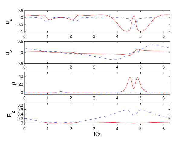
Figure 9: Selected eigenfunction components of the compressible pinch-tearing mode localised on the upper jet. Parameters of the equilibrium are $M_{A}=0.7$, $\beta=0.1$, $d=5$ (see Appendix A), and the perturbation is determined by $\theta_{k}=-\pi/4$ and $k_{x}/K=1$. The growth rate is $\sigma/(v_{0}K)=0.1041+0.6982\,i$. An equivalent mode exists, growing at the same rate, but is localised to the lower jet.

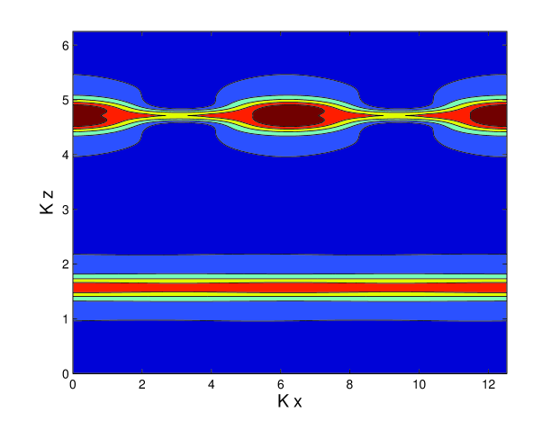
Figure 10: Coloured isocontours of the total density of the compressible pinch-tearing mode in Fig. 9 in the $(x,z)$ plane. The perturbation is normalised so that it is a fifth of the equilibrium density profile. Two periods in the $x$ direction are included.

The most important instabilities we found were the kink mode and the pinch-tearing mode. Importantly, their relative behaviour changes in interesting ways as the plasma beta parameter $\beta\equiv 2c_{s}^{2}/v_{A}^{2}$ varies from large values (the incompressible regime) to low values (narrow compressible channels). In summary, as $\beta$ shrinks (a) instability occurs on significantly shorter horizontal lengthscales, (b) the unstable modes generally localise on one or the other jet, (c) the pinch mode growth rate increases significantly and can reach levels comparable to the kink mode. For certain parameter choices the pinch mode can be the dominant mechanism of channel destruction. In Figs 9 and 10 we plot a representative example of a pinch mode on an extreme compressible channel, so as to compare with our numerical simulations in Section 3.

3 Compressible simulations

So far we have attacked the problem of the MRI’s nonlinear behaviour by reducing it to two linear calculations: that of the MRI channel flow, and that of the parasitic modes which feed on it. In essence, we have concentrated on the life of a single MRI mode and its associated nonlinear solution, while ignoring its possible nonlinear interactions with other MRI modes. In reality, such interactions are inevitable and may prevent the formation of the pure nonlinear channel structures upon which we have based our analyses. In the previous section, we argued that ‘pure’ isolated channels will grow naturally to enormous amplitudes before they collapse — the fact that simulations do not always report this suggests that nonlinear effects early in channel growth are important.

In this section we numerically simulate the equations of nonideal MHD in order to isolate the emergence of parasitic instabilities in various contexts. We then compare the observed behaviour to the predictions of the preceding linear analyses. Concurrently, we discuss the role of the parasites more broadly and make a few comments about the saturation of the MRI and the role of the computational geometry. But first, we review the simulation literature and some conclusions we can draw from it.

3.1 Brief review

Channel flows were discovered in the very first axisymmetric simulations of the MRI in a shearing box (Hawley and Balbus 1992). The box would be dominated initially by the fastest growing MRI channel, but if the vertical wavelength of this solution was smaller than the vertical dimensions of the box the system would witness an inverse cascade to longer wavelength channel flows. (The catalyzing process is perhaps the axisymmetric Type 2 parasitic instability — but see also Tatsuno and Dorland 2008.) Later fully three-dimensional simulations revealed that analogous channel solutions are a recurrent feature of MRI saturation — but only in the case when the imposed $\mathbf{B}$ field exhibits a net flux. Zero net flux runs have never exhibited these coherent structures. Notable works which simulate shearing boxes with a uniform $B_{z}$ are Hawley et al. (1995) and Sano et al. (2004), who work with the equations of compressible ideal MHD, Fleming et al. (2000), Sano and Inutsuka (2001), and Sano (2007), who add resistive dissipation explicitly, and Lesur and Longaretti (2007), who undertake incompressible runs with both resistivity and viscosity.

All these studies employ the classic ‘bar’ computational domain, a box with dimensions $L_{x}\times L_{y}\times L_{z}$, typically elongated in the $y$-direction so that $L_{x}=L_{z}=L$ and $L_{y}=4L$ or $2\pi L$. In this geometry simulations exhibit a pattern of irregular and recurrent ‘bursting’ events whereby two-stream channels form and then collapse in turbulence. For the most part, the amplitudes of these structures are never particularly large, possessing a magnetic pressure of order the thermal pressure at the peak of channel formation. In between the peaks, the disordered troughs possess a magnetic pressure of some tenth the thermal pressure. The troughs are never so low that the linear MRI modes decouple, which means the problem remains stubbornly nonlinear. Exceptions occur when the system is near criticality or, sometimes, in the initial stages of the evolution; in these cases clean isolated channels emerge and reach large amplitudes (Lesur and Longaretti 2007, Section 3.2).

Sano et al. (2004) show that the larger the initial $\beta$ the less prominent the intermittent channel formation; both the amplitudes and frequency of channels drop. In fact, when the imposed field is sufficiently weak ($\beta$ very large) the channels fail to appear at all. The same trend has been shown by Bodo et al. (2008) when they increase the radial size of the computational domain. In both cases (larger $\beta$, larger box) more active MRI modes can fit into the computational domain, and hence a richer nonlinear dynamics is available. We suspect, as a consequence, that the nature of the recurrent channel behaviour is governed by nonlinear interactions between MRI modes, as opposed to linear parasitic behaviour, even if it is usually claimed that parasitic modes (as described in GX and Section 2) are responsible for the channels’ demise. This is explored in more detail in the following subsection.

3.1.1 Channel breakup in bar geometry

We restrict attention here to simulations of recurrent low amplitude channels in the ‘bar’ geometry. The first thing to note is that, according to the incompressible analysis of Section 2, most two-stream channels are stable to the kink mode. Generally, the two-stream channel possesses orientation $\theta\lesssim\pi/4$, and kink modes that are both properly oriented, cf. (14), and which can fit into the computational box, are of too short a wavelength to be unstable (they must have $k<K$). The only exceptions are two-stream MRI channels near marginal stability (as in Fleming et al. 2000 and Lesur and Longaretti 2007) for which $\theta\approx\pi/2$. On the other hand, two stream channels are unstable to the $k_{z}=0$ pinch-tearing mode. It is likely though, owing to their small growth rates ($\sim 0.01\,b\Omega$), that these modes play little role in the dynamics when $b\sim 1$. They should be swamped by the growth of the channel itself, which is at least an order larger. Moreover, simulations of recurrent channels show the breakup takes place on the orbital timescale, which is much shorter, and does not proceed by the formation of plasmoids, etc. Lastly, modes with nonzero $k_{z}$ cannot fit into the computational domain.

One, of course, could argue that the simulated channels possess $b\sim 1$ and hence are outside the jurisdiction of Section 2’s analysis (which requires $b\gg 1$). It may be that shorter wavelength kink instabilities ($k>K$) exist in this regime. But even if this is allowed for, like the resistive pinch modes, nascent kink modes cannot grow faster than their hosts and would therefore not provide a viable way to disrupt the channel. Indeed, we have simulations in larger domains of clean growing channels of low amplitude that remain undisrupted even when vulnerable to kink modes (see Section 3.2.1)

So how are low-amplitude recurrent channels destroyed? The critical issue, in our opinion, is the fact that the repeated two-stream channels emerge from a disordered turbulent trough which is outside the linear regime. For this reason the ‘background’ harbours other MRI modes of appreciable amplitudes which are competing against, and interacting with, the two-stream channel. The two-stream flow eventually dominates but it is highly ‘contaminated’ by its MRI counterparts: perturbations upon it have already achieved nonlinear amplitudes and the clean linear analysis of Section 2, nor a generalisation of it to the $b\sim 1$ regime, is valid. Perhaps it might be fruitful to instead consider the nonlinear stability of the two-channel structure in this situation: short wavelength kink disturbances in this regime may be unstable, in contrast with the linear analysis. Alternatively, we could regard the channel’s destruction simply as a result of turbulent mixing. The eddy turnover time of the MRI-induced turbulence, after all, is of order $\Omega^{-1}$ and hence similar to the growth time of the channel. The latter interpretation is supported by the system’s response to changes in $\beta$ and box size. Increasing either introduces more unstable MRI modes into the box, which enrich the nonlinear turbulent dynamics in the troughs and hence impede the formation and aid the destruction of two-stream channels. Admittedly, the precise details of how these new degrees of freedom work out in practice is not at all straightforward. But whatever the details are, we think it is incorrect to simply attribute channel destruction to a linear ‘parasitic mode’ along the lines of GX or Section 2.

3.2 Numerical results

We now put aside the interesting questions of saturation and concentrate a little on the perhaps more mundane but also more precise and tractable task of exhibiting and examining the parasitic modes as they appear in the simulations. The preceding studies never clearly isolated and revealed the structure of the parasites to which they often appealed. Once this is done, we briefly show simulations of recurrent channels.

Our computations employed a modification of Zeus3D (see Stone and Norman 1992a, b) to solve the equations of nonideal, isothermal, compressible MHD in a shearing box, while assuming an ideal gas law. Dissipation is modelled with an Ohmic resistivity and a Navier-Strokes viscous stress. The equations and numerical set up are described in Lesaffre et al. (submitted).

Dimensions are chosen so that $\Omega=1$, $\rho_{0}=1$, and $L_{z}=1$, where $\rho_{0}$ is the initial mass density and $L_{z}$ is the vertical length of the box. The sound speed is $c_{s}$ and is set to $\sqrt{5/3}$, except for one subsection where it is $10\sqrt{5/3}$. The pressure scale height is $H=c_{s}/\Omega$, and is thus roughly the vertical size of the box in the first case, and more than ten times it in the second. The other parameters are the initial Alfven velocity $v_{A}$, the viscosity $\nu$, and the resistivity $\eta$. These take the values: $\nu=\eta=2\times 10^{-3}$ and $v_{A}=\sqrt{2}/10\approx 0.141$. The plasma $\beta$ is consequently $1.67\times 10^{2}$ (when $c_{s}=\sqrt{5/3}$), or $1.67\times 10^{4}$ (when $c_{s}=10\sqrt{5/3}$). Our choice of $v_{A}$ ensures that the fastest growing channel mode has wavenumber close to $K=2\pi/L_{z}$ and thus exhibits two-stream structure whatever $c_{s}$. No other growing channel solutions fit in the box, though other $k_{x}\neq 0$ modes, and non-axisymmetric ‘modes’, can.

Typically 64 grid cells were used per scale height in the $x$ and $y$ directions and slightly fewer in the $y$ direction. This fixes dissipation above the grid scale. We also conducted runs with 128 grid cells, so as to confirm convergence.

3.2.1 Kink modes

First we exhibit some simulation results that reveal clearly the emergence of the kink instability. For comparison with Section 2 we implement parameters which generate, at least initially, a ‘nearly incompressible’ run. The sound speed is set large with $c_{s}=10\sqrt{5/3}$, and so $\beta=1.67\times 10^{4}$. The computational box is a ‘slab’, with dimensions $4L\times 4L\times L$. The slab geometry is chosen so that those growing kink modes which attack a two-stream channel can fit into the horizontal domain. Finally, the initial condition is an order one amplitude two-stream MRI channel sprinkled with small amplitude perturbations. This choice eliminates muddy nonlinear interactions with other MRI modes and allows the channel to grow and collapse cleanly.

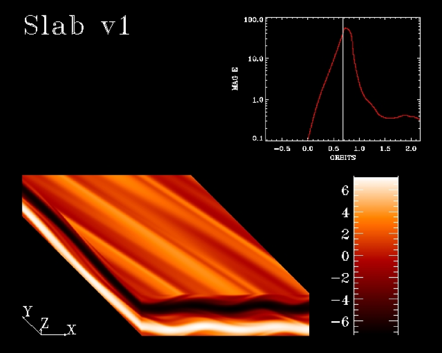
Figure 11: A linear kink mode attacking a two stream solution in slab geometry. The isosurfaces represent the $v_{x}$ component of the solution. In the top right is a graph of the time evolution of the magnetic energy scaled by thermal energy. Note the large magnitude it can achieve before breakdown. Parameters are as stated in the text with $\beta=1.67\times 10^{4}$.

As expected, the two-stream channel grows exponentially to a point and then breaks down. In accordance with the predictions of Section 2.4, the channel achieves large amplitudes before disrupting, even when we increase the amplitude of the perturbations to relatively large values: the channel’s rapid growth helps it ‘outrun’ its parasites, initially. In Fig. 11 we present a coloured 3D plot of the isosurfaces of $v_{x}$ near the peak of the channel growth. We have also inserted a time plot of the total magnetic energy, divided by thermal energy, in the top right corner. As is clear by comparison with Fig. 2, a $k_{z}=0$ kink mode is attacking the two-stream channel, forcing the characteristic sinusoidal pattern on each jet (a few streamers radiating from each peak can also be seen, heralding the coming nonlinear development). The mode possesses $k_{x}/K=1/2$ and $k_{y}/K=1/4$; or rather, $\theta_{k}$ is approximately 26 degrees and $k\approx 0.56$. The channel orientation $\theta$ on the other hand, is near 45 degrees because it is nearly the fastest growing mode (cf. Section 2.2). So the kink mode wavevector is not perfectly aligned with the flow, but its amplitude is nearly optimal for maximum growth. In contrast, parasites that are perfectly aligned with the background flow (and fit into the slab) possess wavenumbers closer to 0.35 and 0.71, which yield growth rates of the same order or less.

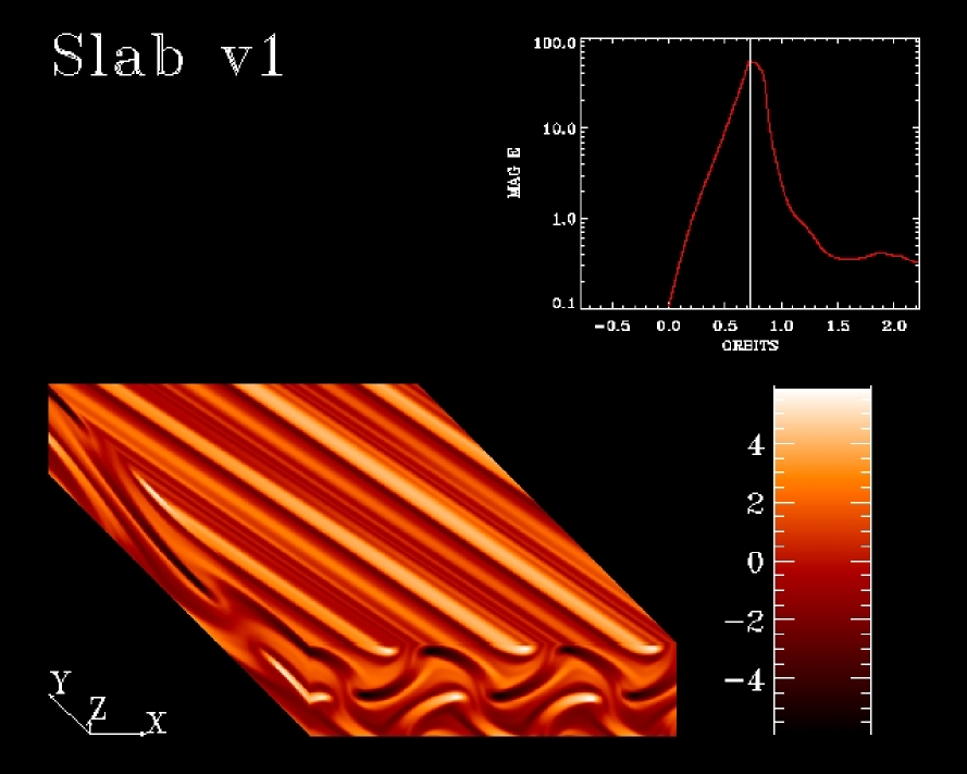
Figure 12: As before but at the nonlinear stage of the kink mode’s evolution and just before the channel’s catastrophic breakdown. Note how the billows have penetrated the adjacent jets.

The ‘billows’ associated with the kink mode grow rapidly but never appear to roll up into a series of ‘cats eye’ vortices. Magnetic field is swept up into each billow and magnetic tension exerts a torque against the vortex’ spin, as has been observed in other studies (Frank et al. 1996, Dahlburg et al. 1997, Biskamp et al. 1998). Before secondary parasitic instabilities destroy these structures they distort the two channels until they interpenetrate each other, fragment, and then disintegrate catastrophically in turbulence. The interpenetration stage, just before break down, is plotted in Fig. 12.

3.2.2 Compressible pinch modes

Next we isolate the compressible pinch mode in a simulation in the classic ‘bar’ geometry: $L\times 4L\times L$. To aid entrance into this regime we assign a lower sound speed $c_{s}=\sqrt{5/3}$ while keeping the Alfvénic speed constant, and so $\beta=1.67\times 10^{2}$. These parameters are shared by the remaining simulations presented in the paper. The initial conditions are set to very low amplitude noise (the early stages of the system’s evolution will select the two-stream channel preferentially and so we need not seed it explicitly).

As expected, the two-stream channel emerges cleanly from the early linear stage of the system’s evolution and continues to grow exponentially in the linear regime. As the amplitude becomes larger we observe the channel structure narrow to two thin planar jets accompanied by large spikes in mass density. The magnetic pressure across each channel is sufficient to efficiently squeeze matter onto the magnetic null surface. This is revealed in Fig. 13, where the variation in density between the troughs and the peaks is more than tenfold. This regime is reached before the slow growing tearing modes of Section 2 (the only unstable modes that can fit in the bar) achieve meaningful amplitudes. Recall that unstable incompressible kink modes cannot fit into the bar geometry because the channel has orientation $\theta\approx\pi/4$ .

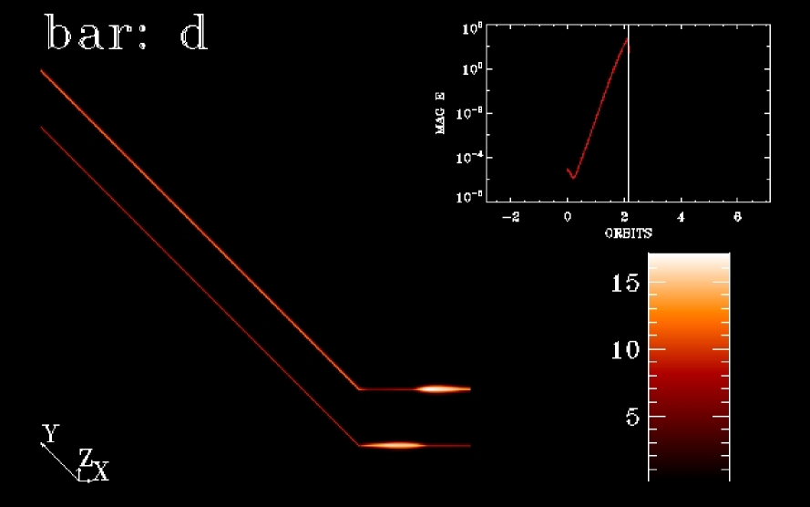
Figure 13: Two axisymmetric linear pinch modes on an extreme channel flow in bar geometry. In this plot the isocontours depict the total density $\rho$. The channel amplitude in this case is enormous, generating a magnetic pressure gradient sufficient to cause the massive variation in $\rho$ between the centre of the jet and the evacuated region outside it. Here the $\beta$ is $1.67\times 10^{2}$.

Once the jets have narrowed sufficiently they become susceptible to fast-growing compressible parasitic instabilities (Section 2.4.2) whose characteristic lengthscale is controlled by the jet width $l$, not the overall channel wavelength $\lambda$. Consistent with Appendix A, the dominant type of mode is the pinch instability, though on occasion it is joined by a compressible kink mode. Typical perturbation profiles of the pinch mode, cf. Fig. 13, correspond relatively well to those examined in the linear theory, cf. Fig. 10. The initial pinching motion subsequently generates a small magnetic island, or plasmoid, which is convected along the jet. As a consequence, the plasmoid adopts the typical ‘droplet’ shape — a leading blunt head and an attenuated tail (Biskamp 2000). Most simulations show that the plasmoids’ growth continues into the nonlinear regime until the perturbation impinges on its neighbouring jet or, as is more common, a fellow plasmoid on the neighbouring jet, at which point the two flows collide and break down in vigorous turbulence. A profile of a nonlinear plasmoid can be observed in Fig. 16 in cube geometry. Those simulations which exhibit the kink mode develop contorted jets more prone to collision.

3.2.3 Recurrent channels

The two preceding runs dealt only with the initial stages of a system’s evolution, in which a clean two-stream solution emerged, reached large amplitudes, and then collapsed due to a parasitic instability. We now turn our attention to what happens next.

After the inaugural outburst, the gas enters a disordered state, periodically organising itself into a turbulent, two-stream structure and then relaxing again. These aftershocks are much smaller than the first burst. In particular, our results agree with the observations of Bodo et al. (2008), confirming that computational boxes that are extended in the $x$-dimension sustain channel bursts of smaller amplitude and frequency. In Figs 14 and 15 we plot channels at the tips of their energy peaks in a bar and a slab when $\beta=1.67\times 10^{2}$. In neither geometry does a two-stream channel achieve much coherence; both suffer large amplitude perturbations even as they grow. But this is a more pronounced in the slab case, where the channel really does struggle to emerge from the turbulent background.

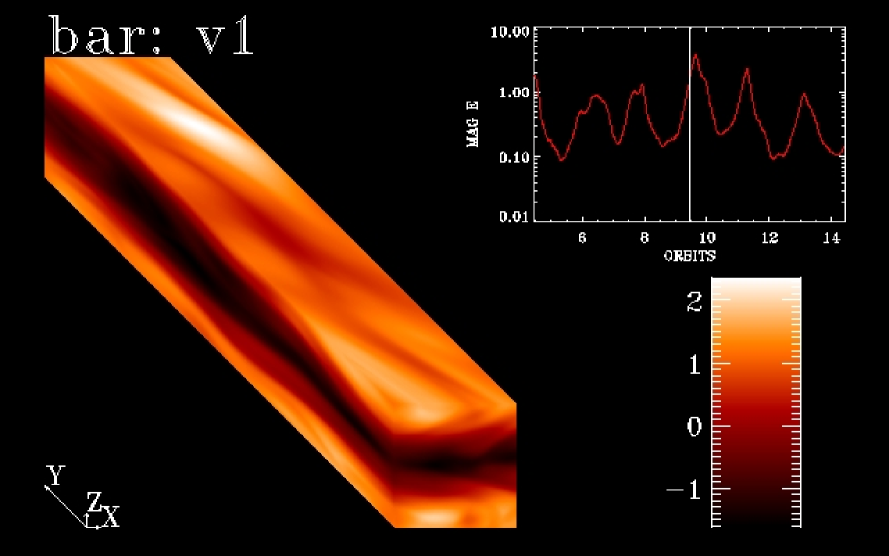
Figure 14: A $v_{x}$ snapshot of a channel peak in the later evolution of the MRI in the bar geometry. The channel is harrassed by large amplitude perturbations during its growth phase and never achieves the pure profiles of the previous cases; eventually it is folded up by the background disordered motions. Here the $\beta$ is $1.67\times 10^{2}$.

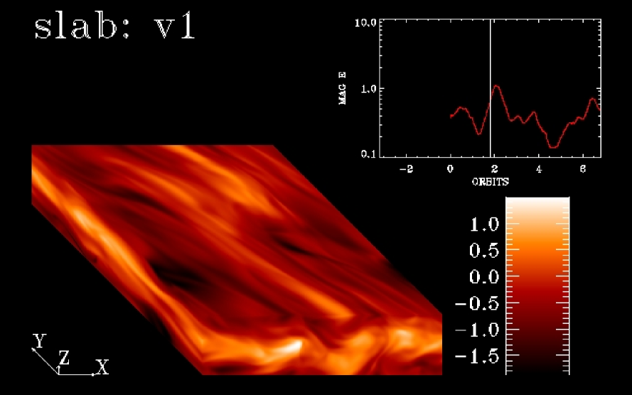
Figure 15: A $v_{x}$ snapshot of a channel peak in the later evolution of the MRI in the slab geometry. The channel emerges with greater difficulty and the perturbations upon it are larger. It is more difficult to sustain coherence in the longer computational domain when turbulence is present. Here the $\beta$ is $1.67\times 10^{2}$.

Though both the channels in Figs 14 and 15 exhibit ‘kinking motions’ it is incorrect to ascribe them to parasitic modes (in the sense of Section 2), as is often done in the literature. Consistent low level turbulence is the salient feature of these runs, and its fluctuations are what ultimately destroy the channel. In slab geometry more nonlinear interactions are available, because more modes can fit into the box, and hence the turbulence more developed. Channels in this case emerge with more difficulty and are destroyed more quickly. (The same behaviour, for the same reasons, proceeds for greater $\beta$.) The large perturbations that the turbulence impresses upon the channel structure are swept into the familiar Kelvin-Helmholtz-like pattern, but this is accordance with the generic vortex dynamics of velocity shear, not the particular dynamics of the linear kink mode. They are then folded-up and thoroughly ‘mixed’ by the turbulent eddies.

In contrast, when we choose parameters close to MRI marginal stability, as when $\beta$ is lowered further, turbulent fluctuations are absent in the troughs (there is only one growing MRI mode). This scenario permits the recurrent formation and growth and destruction of very large-amplitude two-stream channels (cf. Sections 3.2.1 and 3.2.2), as each burst is of the same magnitude as the very first. This eruptive behaviour has been observed in the incompressible simulations of Lesur and Longaretti (2007).

3.2.4 Cube geometry

Lastly, we look at the interesting case of MRI saturation in a cube. The computational domain is set to $L\times L\times L$ and other parameters take the fiducial values of the previous simulations with $\beta=1.67\times 10^{2}$.

In cubes two-stream flows are surprisingly robust and the basic channel structure never breaks down completely. Initially, the gas evolves just as in the bar simulations: a channel grows to a large amplitude and is subsequently attacked by a compressible pinch or kink mode. However, these instabilities do not destroy the structure entirely, instead transforming it into a disordered and fluctuating two-stream flow, characterised by plasmoid-type structures. The key point is that these secondary structures never catastrophically impinge on each other or their neighbouring channels — in fact, for most of the evolution the two streams appear relatively isolated from each other. The restrictive geometry of the cube does not offer sufficient room for the secondary structures to deflect the two jets into each others’ paths, and hence to destroy them. One could say that the channels are ‘stiffened’ by the short periodic boundaries.

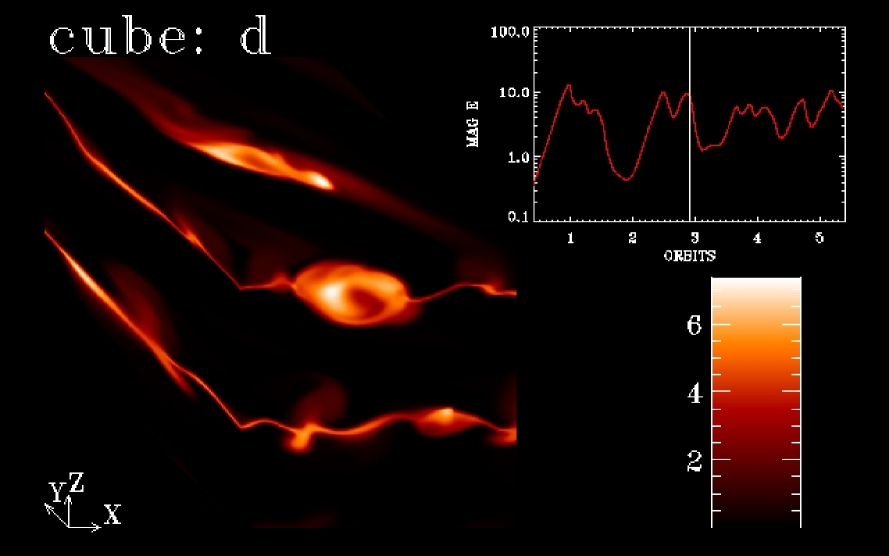
Figure 16: Saturated double jet in cube geometry as represented in density $\rho$. The upper jet exhibits a characteristic feature of the pinch mode’s nonlinear saturation — a fat asymmetrical plasmoid. At future times the lower jet broadens and exhibits wake structures, the characteristic pattern of the saturated kink mode. Here $\beta=1.67\times 10^{2}$.

Fig. 16 presents a snapshot from the saturated two-stream channel. Upon the upper jet travels a nonlinear plasmoid, looking much like the saturated endpoint of the pinch mode in isolated magnetic jets. At later times the lower jet broadens out and radiates ‘wakes’, looking much like the saturated endpoint of the kink mode in a magnetised jet (see Figs 4 and 5 in Biskamp et al. 1998). The appearance and disappearance of these structures is intriguing, and perhaps suggest that the system is oscillating about certain regions of phase space characteristic of magnetic jets more generally (see Balbus and Lesaffre 2008 for more on phase space analyses).

4 Conclusion

We briefly summarise the main results and ideas of the paper. Our principal goal was to understand in greater detail channel flows in the nonlinear saturation of the MRI. We began by revisiting the analysis of GX where we reinterpreted the two classes of parasitic mode that destroy incompressible channels: they can be understood as a ‘double kink mode’ and a hybrid kink-pinch mode, analogues of classic plasma instabilities. Resistivity was added, which slightly increased the growth rates of the latter and introduced slow growing ‘pinch-tearing modes’, both changes a result of the availability of field reconnection.

An important observation made in Section 2 is that, despite this family of parasitic instabilities, an isolated small amplitude channel will inevitably grow to significantly large amplitudes. A channel’s exponential growth allows it to ‘outrun’ nascent parasitic modes until $b\gg 1$, at which point the parasites grow sufficiently fast and overtake their host. Consequently, strong magnetic fields are inevitable whenever a clean channel flow forms: destruction of these flows is then usually due to those parasitic instabilities which can exploit reconnection and so access the fund of energy stored in both the velocity and magnetic shear. These observations are confirmed by numerical simulation in Sections 3.2.1 and 3.2.2.

Next we investigate numerically the recurrent generation and destruction of channels once the initial large amplitude channel is destroyed. The main observation we make here is that channel destruction is qualitatively different from that described by the linear parasite model. Such channels form out of a persistent turbulent flow, whose fluctuations interfere with its development, and ultimately tear it apart. The fact that channel behaviour is weaker when $\beta$ and the radial box are bigger provides evidence for this interpretation, because these changes enrich the nonlinear turbulent dynamics by adding more active MRI modes.

These observations prompt the question: what role do channel solution play in real accretion disks — are they only artefacts of the shearing box’s assumptions? It is too early to answer this conclusively at this point. But a start can be made by incorporating a vertical lengthscale into the problem, such as would issue from vertical stratification. The matter is complicated by the fact that in a stratified disk a linear MRI mode will not generally be a solution to the nonlinear equations. This suggests that isolated channels will never grow to the large amplitudes seen in Sections 3.2.1 and 3.2.2. Once $b\sim 1$, channels must begin interacting with other modes, and the clean channel structure would break down. However, weak recurrent channel behaviour might remain a feature of MRI-induced turbulence in stratified disks, though highly resolved simulations in a semi-local shearing box may be required to reveal them.

Appendix A ‘Extreme channels’ and their parasites

This appendix offers a brief analysis of compressible channels at large amplitudes (‘extreme channels’) and the parasites which beset them. Throughout, $b\gg 1$ is maintained so that the background shear, rotation, and imposed $B_{z}$ field are subdominant. We also assume, as earlier, that the parasitic modes grow at a rate that far outstrips the channel growth and the evolution of its $z$-profile. This permits us to assume a steady background.

We present the main disruption mechanisms of intense compressible channels and compare them with the incompressible case. The qualitative differences can be summarised neatly. When the MRI channels become thinner and more intense the wavelengths of the unstable modes decrease to significantly smaller values. We also find that the modes change their structure and generally localise on one or the other jet. The principle modes are the compressible kink and pinch-tearing modes, and the growth rates of the latter can approach the former as the plasma beta $\beta$ decreases to sufficiently low levels.

In the next subsection we outline the structure of the channel profiles adopted and in the following sketch out the mathematical eigenproblem for the compressible parasites. Once this is done the numerical results are summarised and the main points demonstrated.

A.1 Channel profile

There is no straightforward analytical way to obtain the profile of the compressible channel solution when $\beta$ is small, in contrast to the incompressible case. In this regime, not only will the solution grow exponentially, its $z$-profile will evolve with time as magnetic pressure gradually squeezes the jet into a narrower and narrower layer. Our analysis here is concerned with time-scales much shorter than this evolution, and demonstrates general qualitative points of behaviour. Therefore, we take simple, but well-motivated, approximations.

We consider a compressible channel at a moment in time when its amplitude dwarfs that of the imposed $B_{z}$ field and the background Keplerian shear flow. For convenience, we rotate our $(x,y)$ frame so that $\mathbf{e}_{x}$ points in the direction of the channel flow $\mathbf{v}^{\text{ch}}$. The spatial profiles can then be written as

$$\mathbf{v}^{\text{ch}} =v_{0}\,f(Kz)\,\mathbf{e}_{x}$$ (16)

$$\quad\mathbf{B}^{\text{ch}} =B_{0}\,g(Kz)\,(\mathbf{e}_{x}\,\cos\alpha+\mathbf{e}_{y}\,\sin\alpha),$$ (17)

$$\rho^{\text{ch}} =\rho_{0}\,h(Kz),$$ (18)

where $v_{0}$, $B_{0}$, and $\rho_{0}$ are dimensional constants, $f$, $g$, and $h$ are dimensionless functions, and $K$ is the vertical wavenumber of the channel.

The function $h$ can be related to $g$ if we assume, first, that the gas is isothermal and, second, that to leading order thermal pressure balances magnetic pressure in the $z$-component of the momentum equation. As to the second assumption, in a real simulation the total pressure possesses a small sink centred on each channel which gradually attracts matter: thermal pressure will increase to meet the large magnetic pressure gradients but can never exactly cancel it. This pressure gradient should play a relatively minor role, but may inhibit to some degree the compressible kink mode

We set $P=c_{s}^{2}\,\rho$ where $c_{s}$ is the constant sound speed; then the pressure balance implies

$$h\approx 1+\frac{1}{\beta}\,(1-g^{2}).$$

In so doing we take $\rho_{0}$ to be the density in the nearly evacuated regions between the jets. The plasma beta is defined through $\beta\equiv 2c_{s}^{2}/v_{A}^{2}$.

We employ the following analytic forms:

$$f=\frac{\sinh[d\,\sin Kz]}{\sinh d},\qquad g=\frac{\tanh[d\,\cos Kz]}{\tanh d}.$$ (19)

These profiles introduce the dimensionless parameter $d$ which is the ratio of the channel wavelength $\lambda=2\pi/K$ to the width of the jet, $l$. Thus $d\equiv\lambda/l$. It quantifies the compression of the fluid achieved by the magnetic pressure. It hence depends on $\beta$. Roughly, the smaller $\beta$ the greater the compression and hence the greater $d$. The profile choices above may not be immediately obvious but have the nice property that they connect naturally to the incompressible channels of Section 2 in the double limit $\beta,\,d^{-1}\gg 1$, on one hand, and the discontinuous current sheets, examined by GX, in the limit $\beta,\,d^{-1}\ll 1$, on the other. What remains undetermined are the relationships between $v_{0}$, $K$, $B_{0}$, which require solution of the nonlinear equations, something that can be accomplished in each limit but is difficult in between.

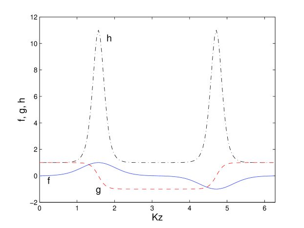
Figure 17: Plotted here are the dimensionless functions $f(Kz)$, $g(Kz)$, and $h(Kz)$ which characterise our approximation to the compressed channel solution. The parameters employed are $d=5$ and $\beta=0.1$. Note that the inward and outward jets are centred at $Kz=\pi/2$ and $3\pi/2$, altitudes which coincide with the magnetic null surfaces and the density maxima.

A.2 Parasitic modes

The approximate channel profiles introduced above are now perturbed by a small disturbance. We assume that these parasitic modes possess a growth rate of order the channel amplitude and thus we neglect the temporal evolution of the channel and the small $B_{z}$ and $v_{z}$ field associated with its gradual vertical compression. As earlier, we set

$$\mathbf{v}=\mathbf{v}^{\text{ch}}+\mathbf{v}^{\prime},\qquad\mathbf{B}=\mathbf{B}^{\text{ch}}+\mathbf{B}^{\prime},\qquad\rho=\rho^{\text{ch}}+\rho^{\prime},$$

linearise in the perturbations, and search for modes of the form $\propto e^{ik_{x}x+ik_{y}y+\sigma t}$. Next we choose units so that $K=1$, $v_{0}K=1$. The perturbations are scaled by $\rho_{0}$, $v_{0}$, and $B_{0}$. The governing compressible equations are now

$$\sigma\mathbf{v}^{\prime}=-i(\mathbf{k}\cdot\mathbf{v}^{0})\mathbf{v}^{\prime}-\partial_{z}\mathbf{v}^{0}\,v_{z}^{\prime}-\frac{1}{M^{2}\,h}(i\mathbf{k}+\mathbf{e}_{z}\partial_{z})\rho^{\prime}$$

$$\hskip 25.6073pt+\frac{1}{M_{A}^{2}\,h}\left\{i(\mathbf{k}\cdot\mathbf{B}^{0})\mathbf{B}^{\prime}+\partial_{z}\mathbf{B}^{0}\,B_{z}^{\prime}-(i\mathbf{k}+\mathbf{e}_{z}\partial_{z})(\mathbf{B}^{0}\cdot\mathbf{B}^{\prime})\right\}$$

$$\sigma\mathbf{B}^{\prime}=\left\{i(\mathbf{k}\cdot\mathbf{B}^{0})\mathbf{v}^{\prime}-i(\mathbf{k}\cdot\mathbf{v}^{0})\mathbf{B}^{\prime}\right\}+\left\{\partial_{z}\mathbf{v}^{0}\,B_{z}^{\prime}-\partial_{z}\mathbf{B}^{0}\,v_{z}^{\prime}\right\}$$

$$\hskip 71.13188pt-\left\{i(\mathbf{k}\cdot\mathbf{v}^{\prime})+\partial_{z}v_{z}^{\prime}\right\}\,\mathbf{B}^{0}-\frac{1}{R_{m}}\,(k^{2}-\partial_{z}^{2})\mathbf{B}^{\prime}$$

$$\sigma\rho^{\prime}=-i(\mathbf{k}\cdot\mathbf{v}^{0})\rho^{\prime}-(\partial_{z}h)\,v_{z}^{\prime}-h\left\{i(\mathbf{k}\cdot\mathbf{v}^{\prime})+\partial_{z}v_{z}^{\prime}\right\},$$

where most of the notation is carried over from Section 2.2 apart from the Mach number which is defined through

$$M=\frac{v_{0}}{c_{s}}$$

and the magnetic Reynolds number which we define differently

$$R_{m}=\frac{v_{0}}{\eta K}.$$

Note that $\beta=2M^{2}/M_{A}^{2}$. Finally, the equilibrium fields are given by

$$\mathbf{v}^{0}=f(z)\,\mathbf{e}_{x},\qquad\mathbf{B}^{0}=g(z)\,(\mathbf{e}_{x}\,\cos\alpha+\mathbf{e}_{y}\,\sin\alpha).$$

In the above, the incompressibility constraint has been replaced by the full continuity equation: $\partial_{t}\rho+\nabla\cdot(\rho\mathbf{v})=0$.

As in Section 2, we have a Floquet boundary value problem and so assume the Floquet ansatz and boundary conditions. This completes the statement of the problem. The task now is to compute the growth rates $\sigma$ and associated eigenfunctions given the following parameters: $M$, $M_{A}$, $R_{m}$, $\alpha$, and $d$, on one hand, and $k_{x}$, $k_{y}$, and $k_{z}$, on the other.

A.3 Numerical results

We numerically solve the linear eigenvalue problem using a Fourier pseudo-spectral method (Boyd 2000). This approach supplies us with an approximation to the full spectrum for the given parameters. There are unfortunately eight parameters, quite a number, and their various influences can obscure the main points we would like to make. Therefore, only a few combinations are considered, those that are most representative and which demonstrate the essential behaviour.

First, we examine modes which appear in two-channel flows in a periodic box; in this domain there is sufficient vertical space only for $k_{z}=0$ modes. Next we set $\alpha=-\pi/2$, so the $\mathbf{B}$ field is perpendicular to the $\mathbf{v}$ field. In practice, because of finite $R_{m}$, this angle will be slightly less but the effect we believe is small and warrants neglect. Also we set $R_{m}=500$, a representative value. As for the Alfvénic Mach number, channel flows appear in MRI linear theory and in nonlinear simulations as slightly sub-Alfvénic, hence we set $M_{A}$ to values between 0.5 and 1. These choices still leave four parameters parameters: $\beta$ (or $M$), $d$, and $k_{x}$ and $k_{y}$. The latter two we replace by magnitude and angle, $k$ and $\theta_{k}$.

A.3.1 Compressible kink modes

As in the incompressible case, the kink mode favours wavevectors oriented along the background channel flow, $\theta_{k}=0$. When $d$ takes very small and $\beta$ very large values we obtain the same modes and behaviour as in Section 2, the only difference being in the scaling. As we increase $d$ and decrease $\beta$ we enter the compressible regime and the behaviour of the kink mode changes in a number of ways.

First, the thinner channels allow instability on a wider range of lengthscales, and the scale of the fastest growing mode decreases. In the incompressible limit the fastest growing mode possesses $k\approx 0.6$, while in the regime associated with $d=10$, $\beta=0.05$ the fastest growing mode possesses $k\approx 1.6$.

Second, the structure of the kink mode alters, particularly on the newly unstable shorter scales. In the incompressible case, the kink mode attacked both channels concurrently. In the compressible case, higher $k$ kink modes localise on one or the other channel and thus appear in complex conjugate pairs (similar to the Type 2 and the pinch-tearing modes of Section 2). However, kink modes of long horizontal wavelength cannot support this vertical localisation and at a critical (small) $k$ the two modes ‘detach’ from each other, take different growth rates, and attack both channels concurrently.

Lastly, the growth rate of the mode does not alter significantly. At smaller $\beta$ (and hence larger $M$) extra work must be expended in deforming the compressible plasma, but at smaller $\beta$ we take larger $d$ and so the jet is also thinner and exhibits a greater vertical shear, exacerbating instability. The two effects appear to roughly cancel.

A.3.2 Compressible pinch-tearing modes

The compressible pinch-tearing mode appears for all orientations of $\theta_{k}$. On decreasing $d$ it transforms naturally into the $k_{z}=0$ incompressible pinch-tearing mode explored in Section 2.3.4. In contrast to the incompressible case, for general $d$ the compressible mode exists for orientations perpendicular to $\mathbf{B}^{\text{ch}}$. It hence resembles the pinch modes exhibited in other studies (Wang et al. 1988, Biskamp et al. 1998).

The structure of the mode is much the same as in Section 2, though the localisation is far more pronounced when $d$ is large. This is seen in Figs 9 and 10 where we plot a representative mode for $d=10$, $\beta=0.1$. There are two other striking changes as we approach the compressible, large $d$ low $\beta$ limit.

First, the mode grows on a very large range of wavelengths, down to scales of order $(Kd)^{-1}$, which reveals that it is strongly influenced by the jet width. As a consequence, the fastest growing mode possesses a significantly shorter wavelength than that of the overall channel structure $\lambda$ (and about half that of the fastest growing kink mode).

Second, the maximum growth rate is significantly larger in the compressible regime. The pinch mode can grow as fast as the kink mode for a wide range of parameters, in contrast to Section 2. The dominance of the pinch mode at low $\beta$ (large $d$) has been reported by Wang et al. (1988) for an isolated current sheet, which is the case in our analysis for certain parameters. The rapid growth of the pinch mode at small $\beta$ is due primarily to the thinness of the jets, a configuration that greatly facilitates the reconnection of magnetic field: because oppositely directed field lines are physically so much closer it requires less work to draw them together and break them. Hence, the increased growth rates of the pinch instability reflect the ease with which the modes can access the fund of energy stored in the background magnetic shear.

References

- (1) Balbus, S. A., Hawley, J. F., 1991. ApJ, 376, 214.
- (2) Balbus, S. A., Hawley, J. F., 1998. Rev. Mod. Phys., 70, 1.
- (3) Balbus, S. A., Lesaffre, P., 2008. New Astron. Rev., 51, 814.
- (4) Bickley, W. G., 1937. Phil. Mag., 23, 727.
- (5) Biskamp, D., 2000. Magnetic Reconnection in Plasmas. Cambridge Univ. Press, Cambridge.
- (6) Biskamp, D., Schwarz, E., Zeiler, A., 1998. Phys. Plasmas, 5, 2485.
- (7) Bodo, G., Mignone, A., Cattaneo, F., Rossi, P., Ferrari, A., 2008. A&A, 487, 1.
- (8) Boyd, J. P., 2000. Chebyshev and Fourier Spectral Methods (2nd ed.). Dover Publications, New York.
- (9) Chandrasekhar, S., 1961. Hydrodynamic and Hydromagnetic Stability. Dover Publications, New York.
- (10) Dahlburg, R. B., Boncinelli, P., Einaudi, G., 1997. Phys. Plasmas, 4, 1997.
- (11) Drazin, P. G., Reid, W. H., 1981. Hydrodynamic Stability. Cambridge Univ. Press, Cambridge, UK.
- (12) Fleming, T. P., Stone, J. M., Hawley, J. F., 2000. ApJ, 530, 464.
- (13) Frank, A., Jones, T. W., Ryu, D., Gaalaas, J. B., 1996. ApJ, 460, 777.
- (14) Fromang, S., Papaloizou, J., Lesur, G., Heinemann, T., 2007. A&A, 476, 1123.
- (15) Goldreich, P., Lynden-Bell, D., 1965. MNRAS, 130, 125.
- (16) Goodman, J., Xu, G., 1994. ApJ, 432, 213.
- (17) Hawley, J. F, 2000. ApJ, 528, 462.
- (18) Hawley, J. F., Balbus, S. A., 1992. ApJ, 400, 595.
- (19) Hawley, J. F, Gammie, C. F., Balbus, S. A, 1995. ApJ, 440, 742.
- (20) Lesaffre, P., Balbus, S. A., 2007. MNRAS, 381, 319.
- (21) Lesaffre, P., Balbus, S. A., Latter, H. N., 2009. Submitted to MNRAS.
- (22) Lesur, G., Longaretti, P-Y., 2007. MNRAS, 378, 1471.
- (23) Pessah, M. E., Chan, C., Psaltis, D., 2007. ApJ, 668, L51.
- (24) Pessah, M. E, Chan, C., 2008. ApJ, 684, 498.
- (25) Pritchett, P. L., Lee, Y. C., Drake, J. F., 1980. Phys. Fluids, 23, 1368.
- (26) Sano, T., 2007. Ap&SS, 307, 191.
- (27) Sano, T., Miyama, S. M, 1999. ApJ, 515, 776.
- (28) Sano, T., Inutsuka, S., 2001. ApJ, 561, L179.
- (29) Sano, T., Inutsuka, S., Turner, N. J.; Stone, J. M., 2004. ApJ, 605, 321.
- (30) Stone, J. M., Norman, M. L., 1992a. ApJS, 80, 753.
- (31) Stone, J. M., Norman, M. L., 1992b. ApJS, 80, 791.
- (32) Tatsuno, T., Dorland, W., 2008. Astron. Nachr., 329, 688.
- (33) Wang, S., Lee, L. C., Wei, C. Q., Akasofu, S.-I., 1988. Sol. Phys., 117, 157.
- (34) White, R. B., 1986. Rev. Mod. Phys, 58, 183.