Multi-mode states in decoy-based quantum key distribution protocols

Abstract

Every security analysis of quantum key distribution (QKD) relies on a faithful modeling of the employed quantum states. Many photon sources, like for instance a parametric down conversion (PDC) source, require a multi-mode description, but are usually only considered in a single-mode representation. In general, the important claim in decoy-based QKD protocols for indistinguishability between signal and decoy states does not hold for all sources. We derive new bounds on the single photon transmission probability and error rate for multi-mode states, and apply these bounds to the output state of a PDC source. We observe two opposing effects on the secure key rate. First, the multi-mode structure of the state gives rise to a new attack that decreases the key rate. Second, more contributing modes change the photon number distribution from a thermal towards a Poissonian distribution, which increases the key rate.

I Introduction

The security of classical cryptography is based on the high computational complexity of the decryption process combined with the condition that the adversary only has a limited amount of computational power. In contrast, quantum key distribution (QKD) allows two parties, Alice and Bob, to share a secret key that is inaccessible to an eavesdropper Eve whose power is only limited by the laws of quantum physics. In 1984, Bennett and Brassard introduced the first QKD protocol BB84 Bennett1984 . It is still the most commonly used protocol, although many more have been proposed since then Gisin2002 ; Duvsek2006 ; Mauerer2008a .

This first theoretical proposal assumed perfect devices, namely single-photon sources and error-free transmission and detection. With the development of sophisticated security proofs, these restrictions could gradually be lessened. First, security has been proved in the presence of noise Mayers1998 ; Shor2000 . In the next step, the necessity of single-photon sources has been taken out of the equation Gottesman2004 . This, however, reduced the achievable key rate drastically, because multiphoton events give rise to the photon number splitting (PNS) attack Lutkenhaus2000 ; Brassard2000 ; Lutkenhaus2002 , which Alice and Bob cannot distinguish from natural losses.

This issue can be resolved with the decoy method, which was introduced by Hwang Hwang2003 , and has been further developed to a practically realizable form by several researchers Lo2005 ; Wang2005a ; Ma2005 . In this method, additional decoy states with a different photon number distribution than the primary signal states are randomly introduced. It is crucial that decoy states share all other physical characteristics of the signal so that Eve cannot distinguish between decoy and signal. Consequently, the decoys are affected by the PNS attack in the same way as the signal states, and this perturbation of the system reveals Eve’s presence. Since Eve has to design her attack in a way that cannot be detected by Alice and Bob (otherwise the protocol is aborted), her attack possibilities are drastically limited when she is confronted with a decoy protocol. This enables Alice and Bob to achieve an improved key rate.

The important assumption that Eve cannot distinguish between photons arising from signal and decoy states is trivially fulfilled for a single-mode description where all photons are created by the same creation operator. However, this model does not match experimental reality well. Hence, in this paper, we treat the scenario where photons are excited into many different modes and the excitation probability for each mode differs between signal and decoy states. This multi-mode description is, for instance, necessary for a realistic representation of the states created by a parametric down conversion (PDC) source, in which case the different modes correspond to different spectral modes Mauerer2008 .

This paper is organized as follows. In Sec. II, we review the decoy method and introduce the notation necessary for the subsequent analysis. Sec. III presents the description of a multi-mode state with special emphasis on spectral modes for the description of a PDC state. In Sec. IV and V, we describe new attack possibilities when multi-mode states are used and derive new bounds that allow us to calculate the achievable key rate in this scenario. Sec. VI finally applies the analysis to the multimode PDC state and gives new bounds on the achievable key rate.

II Decoy Method

The security of BB84 is based on the no-cloning theorem Wootters1982 , which prevents Eve from making a copy of a transmitted single photon. However, the security argument is not applicable to multiphoton events, because for these events Alice implicitly encodes the same information on all photons in the pulse. This, in turn, allows Eve to obtain an identical copy of Bob’s state by splitting away one of the photons. Hence only detection events arising from single photons give a positive contribution to the secure key rate. With current technology, Alice is not able to determine the number of photons her source emitted. Thus Alice and Bob cannot simply ignore multiphoton events. In this scenario, a lower bound on the secure key rate $S$ is given by Gottesman2004 ; Lo2005

$$S\geq q\left[Y_{1}^{(\mathrm{s})}p_{1}^{(\mathrm{s})}\left(1-H(e_{1}^{(\mathrm{s})})\right)-Q^{(\mathrm{s})}f(E^{(\mathrm{s})})H(E^{(\mathrm{s})})\right].$$ (1)

Here $p_{n}^{(\mathrm{s})}$ ($n\in\mathbb{N}_{0}$) denotes the photon number distribution of Alice’s source, $f(E^{(\mathrm{s})})$ is the error correction efficiency, $H(x)=-x\log(x)-(1-x)\log(1-x)$ is the binary Shannon entropy and $q$ accounts for incompatible basis choices of Alice and Bob. In the standard BB84 protocol, $q=1/2$. The overall detection probability is given by the gain

$$Q^{(\mathrm{s})}=Y_{0}p_{0}^{(\mathrm{s})}+Y_{1}^{(\mathrm{s})}p_{1}^{(\mathrm{s})}+Y_{\mathrm{M}}^{(\mathrm{s})}p_{\mathrm{M}}^{(\mathrm{s})},$$ (2)

where the yields $Y_{0}^{(\mathrm{s})}$, $Y_{1}^{(\mathrm{s})}$ and $Y_{\mathrm{M}}^{(\mathrm{s})}$ are the detector click probabilities conditioned on emitted zero-, one-, and multiphoton events of Alice’s source, respectively. Analogously, the zero-, one- and multi-photon error rates, $e_{0}$, $e_{1}$ and $e_{\mathrm{M}}$, are defined as the error rates conditioned on emitted zero-, one-, and multiphoton events, respectively. The relation to the total quantum bit error rate (QBER) $E^{(\mathrm{s})}$ is given by

$$Q^{(\mathrm{s})}E^{(\mathrm{s})}=e_{0}Y_{0}p_{0}^{(\mathrm{s})}+e_{1}^{(\mathrm{s})}Y_{1}^{(\mathrm{s})}p_{1}^{(\mathrm{s})}+e_{\mathrm{M}}^{(\mathrm{s})}Y_{\mathrm{M}}^{(\mathrm{s})}p_{\mathrm{M}}^{(\mathrm{s})}.$$ (3)

The QBER and the gain $Q^{(\mathrm{s})}$ are directly accessible from the recorded data of the QKD protocol. However, since Alice and Bob do not know when a single photon was sent, they cannot determine the exact values of $Y_{1}^{(\mathrm{s})}$ and $e_{1}^{(\mathrm{s})}$, but need to estimate them using worst-case assumptions. Prior to the decoy method, they had to assume that all multiphoton events produce a click at Bob’s detector. This corresponds to $Y_{\mathrm{M}}^{(\mathrm{s})}=1$, and a lower bound on $Y_{1}^{(\mathrm{s})}$ can be calculated with Equation (2). This estimate, however, lies well below the single photon transmission probability caused by natural losses. In addition, Alice and Bob have to assume that all errors arise from single photon events, resulting in a very high estimate of $e_{1}^{(\mathrm{s})}$. These values are actually achieved if Eve performs a photon number splitting (PNS) attack Lutkenhaus2000 ; Brassard2000 ; Lutkenhaus2002 , and lead to a drastically reduced key rate Gottesman2004 .

The decoy method enables Alice and Bob to attain better estimates of $Y_{1}^{(\mathrm{s})}$ and $e_{1}^{(\mathrm{s})}$. This is achieved by randomly introducing “decoy” states with independent photon number distributions. For each photon number distribution, the gain and QBER can be determined individually, resulting in better bounds on $Y_{1}^{(\mathrm{s})}$ and $e_{1}^{(\mathrm{s})}$.

In this paper, we base our analysis on the so-called vacuum+weak decoy method Wang2005a ; Ma2005 , which uses two decoy states. Deliberately interspersing the signal stream with vacuum states ($p_{n}=\delta_{n0}$, gain $Q=Y_{0}$) allows Alice and Bob to determine the dark count probability $Y_{0}$. The second decoy state is of low intensity and features a photon number distribution $p_{n}^{(\mathrm{d})}$ that differs from the photon number distribution $p_{n}^{(\mathrm{s})}$ of the regular signal. In the following, we will refer to this state as the decoy state, and to the state with photon number distribution $p_{n}^{(\mathrm{s})}$ as the signal state. The gain for the decoy state is given by

$$Q^{(\mathrm{d})}=Y_{0}p_{0}^{(\mathrm{d})}+Y_{1}^{(\mathrm{d})}p_{1}^{(\mathrm{d})}+Y_{\mathrm{M}}^{(\mathrm{d})}p_{\mathrm{M}}^{(\mathrm{d})},$$ (4)

with the yields defined equivalently to the signal yields. The yield $Y_{0}$ for an emitted zero-photon state has to be the same for all states because Eve cannot distinguish between vacua arising from different states. However, there is no a priori reason for the single- and multiphoton yields to be the same for signal and decoy. In the analyses up to now, it was assumed that Eve cannot distinguish between $n$-photon events arising from signal and decoy state, resulting in $Y_{n}^{(\mathrm{s})}=Y_{n}^{(\mathrm{d})}$ ($n\in\mathbb{N}_{0}$). Note that this is the assumption we will loosen in Section IV, as it is generally not justified in a multi-mode description of the states. However, proceeding with $Y_{n}^{(\mathrm{s})}=Y_{n}^{(\mathrm{d})}$, from Equations (2) and (4) the lower bound

$$Y_{1,\mathrm{LB}}=\frac{p_{2}^{(\mathrm{s})}}{p_{2}^{(\mathrm{s})}p_{1}^{(\mathrm{d})}-p_{1}^{(\mathrm{s})}p_{2}^{(\mathrm{d})}}\times\\ \Bigg{(}Q^{(\mathrm{d})}-\frac{p_{2}^{(\mathrm{d})}}{p_{2}^{(\mathrm{s})}}Q^{(\mathrm{s})}-\frac{p_{2}^{(\mathrm{s})}p_{0}^{(\mathrm{d})}-p_{0}^{(\mathrm{s})}p_{2}^{(\mathrm{d})}}{p_{2}^{(\mathrm{s})}}Y_{0}\Bigg{)}$$ (5)

on the signal single photon yield can be derived if the additional condition

$$\frac{Y_{\mathrm{M}}^{(\mathrm{d})}}{Y_{\mathrm{M}}^{(\mathrm{s})}}\leq\frac{p_{2}^{(\mathrm{d})}/p_{\mathrm{M}}^{(\mathrm{d})}}{p_{2}^{(\mathrm{s})}/p_{\mathrm{M}}^{(\mathrm{s})}}$$ (6)

is satisfied. This is, for instance, fulfilled if both signal and decoy have a Poissonian or thermal distribution with a lower mean photon number for the decoy distribution.

With a similar Equation to (3) for the decoy QBER (i.e., $(.)^{(\mathrm{s})}\rightarrow(.)^{(\mathrm{d})}$), an upper bound on the single photon error rate of the decoy state can be calculated as

$$e_{1}^{(\mathrm{d})}\leq e_{1,\mathrm{ub}}^{(\mathrm{d})}=\frac{1}{p_{1}^{(\mathrm{d})}Y_{1,\mathrm{LB}}^{(\mathrm{d})}}\left[E^{(\mathrm{d})}Q^{(\mathrm{d})}-e_{0}Y_{0}p_{0}^{(\mathrm{d})}\right].$$ (7)

The postulated indistinguishability of $n$-photon states for signal and decoy gives $e_{1,\mathrm{ub}}^{(\mathrm{s})}=e_{1,\mathrm{ub}}^{(\mathrm{d})}$ and $Y_{1,\mathrm{LB}}^{(\mathrm{d})}=Y_{1,\mathrm{LB}}^{(\mathrm{s})}$, because $Y_{1}^{(\mathrm{d})}=Y_{1}^{(\mathrm{s})}$, and $e_{0}=1/2$, since a dark count gives the wrong result 50% of the time.

The derived bounds, Equations (5) and (7), are much tighter than the worst case assumptions without decoy states. Therefore using them in Equation (1) results in a significant improvement in the achievable secure key rate Lo2005 .

III The Multi-Mode State

QKD analyses generally assume that Alice’s output states are accurately represented by a single-mode description as

$$\rho^{(\mathrm{s/d})}=\sum_{n}p^{(\mathrm{s/d})}(n)\ket{n}\bra{n},$$ (8)

where $p^{(\mathrm{s/d})}(n)$ denotes the signal and decoy photon number distributions.

This form intrinsically implies that all emitted photons have identical properties, in particular they are all excited into the same spectral mode. This appears as an appropriate modeling for weak coherent pulses emitted by a laser as multi-mode effects can be expected to be less critical. However, designing a PDC source with single-mode emission is a complex task, as it requires two output beams with independent spatio-spectral mode structures Mosley2008 .

A type-II PDC process emits photons in two different polarization modes, called signal and idler. The photon numbers in signal and idler modes are strictly correlated. If PDC sources are used in ”prepare and measure” QKD protocols, only the photons of the signal mode are employed for information encoding. Describing the PDC output state in a single-mode description as $\ket{\Psi^{(\mathrm{s/d})}}=\sum_{n}c^{(\mathrm{s/d})}(n)\ket{n}_{\mathrm{s}}\ket{n}_{\mathrm{i}}$, we can obtain signal states of the form of Equation (8) by tracing over the idler mode.

A more realistic model of the PDC output state has to account for the multi-mode structure as follows Mauerer2008 :

$$\ket{\Psi^{(\mathrm{s/d})}}=\bigotimes_{k=1}^{N}\sum_{n}c^{(\mathrm{s/d})}(k,n)\ket{n,\xi_{k}}_{\mathrm{s}}\ket{n,\zeta_{k}}_{\mathrm{i}}$$ (9)

with

$$\ket{n,\xi_{k}}_{\mathrm{s}}=\frac{1}{\sqrt{n!}}\left(A_{\mathrm{s},\xi_{k}}^{\dagger}\right)^{n}\ket{0},$$ (10)

$$A_{\mathrm{s},\xi_{k}}^{\dagger}\equiv\int\mathrm{d}\omega\xi_{k}(\omega)a^{\dagger}_{\mathrm{s}}(\omega).$$ (11)

Equation (10) describes a state with $n$ photons in the spectral mode $\xi_{k}(\omega)$. Here $\xi_{k}(\omega)$ is a set of orthonormal functions, therefore the orthonormality condition $\braket{n,\xi_{i}}{m,\xi_{j}}=\delta_{nm}\delta_{ij}$ holds. For a detailed description of this notation, see Rohde2007 . Note that we consider only one spatial mode in Equation (9), which can be achieved by using a single mode fiber. The following analysis, however, does not depend on the mode type and thus can also be applied to states with more than one spatial mode.

Tracing out the idler mode gives the state

$$\rho^{(\mathrm{s/d})}=\bigotimes_{k=1}^{N}\sum_{n}p^{(\mathrm{s/d})}(k,n)\ket{n;\xi_{k}}\bra{n;\xi_{k}}$$ (12)

with $p^{(\mathrm{s/d})}(k,n)=|c^{(\mathrm{s/d})}(k,n)|^{2}=\operatorname{sech}^{2}r_{k}^{(\mathrm{s/d})}\tanh^{2n}r_{k}^{(\mathrm{s/d})}$ in the signal arm Mauerer2008 . Here the squeezing parameter $r_{k}^{(\mathrm{s/d})}\propto\sqrt{I^{(\mathrm{s/d})}}$ is proportional to the square root of the pump intensity. Hence, if signal and decoy states are created by pumping the crystal with different intensities, the mode distributions for signal and decoy states will be different and our multi-mode treatment becomes essential.

In our numerical simulations, Section VI, we will return to investigating the PDC state to illustrate the multi-mode effects in decoy-based QKD systems. Note, however, that the following analysis applies to all states of the form (12) and is by no means restricted to a PDC source or spectral modes.

IV New Bound on $Y_{1}^{(\mathrm{s})}$

Recall that in a single mode description, the yields for $n$-photon signal and decoy states are identical and thus a lower bound on $Y_{1}^{(\mathrm{s})}$ can be computed by Equation (5) from the known gains and photon number distributions.

In this section, we develop a means of computing a lower bound on $Y_{1}^{(\mathrm{s})}$ for multi-mode states as defined in Equation (12). For states of this type, $Y_{n}^{(\mathrm{s})}=Y_{n}^{(\mathrm{d})}$ is no longer valid for $n\geq 1$. Note, however, that $Y_{0}$ is still the same for signal and decoys, because for zero emitted photons the resulting state is always described by the same vacuum state and thus Eve cannot treat these pulses differently for signal and decoys. The derivation of the new lower bound on $Y_{1}^{(\mathrm{s})}$ proceeds in three steps. First, we derive a lower bound on the signal single-photon yield $Y_{1}^{(\mathrm{s})}$ for a given decoy single-photon yield $Y_{1}^{(\mathrm{d})}$. Then, we determine an upper bound on the decoy multiphoton yield $Y_{\mathrm{M}}^{(\mathrm{d})}$ for a given signal multiphoton yield $Y_{\mathrm{M}}^{(\mathrm{s})}$. Finally, with these two relations, we are able to calculate a lower bound on $Y_{1}^{(\mathrm{s})}$ for given signal and decoy gains, $Q^{(\mathrm{s})}$ and $Q^{(\mathrm{d})}$.

Step 1 - Lower bound on $Y_{1}^{(\mathrm{s})}$ for a given $Y_{1}^{(\mathrm{d})}$: Assume Eve has to let a certain fraction $Y_{1}^{(\mathrm{d})}$ of the decoy single-photon events pass to achieve the desired decoy gain. In this step, we are seeking the lowest possible value for the signal single-photon yield $Y_{1}^{(\mathrm{s})}$ that is compatible with the given $Y_{1}^{(\mathrm{d})}$. Using Equation (12), we find the conditioned one-photon state to be

$$\rho_{1}^{(\mathrm{s/d})}=\sum_{k}m_{k}^{(\mathrm{s/d})}\ket{1;\xi_{k}}\bra{1;\xi_{k}},$$ (13)

where we define the mode occupation probabilities by

$$m_{k}^{(\mathrm{s/d})}=\frac{p^{(\mathrm{s/d})}(k,1)\prod_{i\neq k}p^{(\mathrm{s/d})}(i,0)}{{P_{1}^{(\mathrm{s/d})}}},$$ (14)

and the single-photon probability is given by

$$P_{1}^{(\mathrm{s/d})}=\sum_{k}p^{(\mathrm{s/d})}(k,1)\prod_{i\neq k}p^{(\mathrm{s/d})}(i,0).$$ (15)

We have to assume that Alice does not have the technology to determine in which mode a photon resides. Remember that she cannot even determine the total number of emitted photons for a given event. However, an apparatus that measures the number of photons in each mode individually is possible in principle, because all modes are orthogonal. Therefore, if we want to claim unconditional security, we have to give Eve knowledge about how many photons each mode contains. For the single-photon case, this means that she knows in which mode the photon is. This, in turn, allows Eve to reach different single-photon yields for signals and decoys by selectively blocking modes if the mode occupation probabilities $m_{k}$ differ for signal and decoy state.

Figure 1 illustrates how this can be accomplished for the case of two different modes with $m_{1}^{(\mathrm{d})}=0.7$, $m_{2}^{(\mathrm{d})}=0.3$, $m_{1}^{(\mathrm{s})}=0.6$ and $m_{2}^{(\mathrm{s})}=0.4$. If Eve blocks all photons in the second mode, 70% of the decoy single-photons event are transmitted, but only 60% of the signal single-photons pass through the channel. This results in the yields $Y_{1}^{(\mathrm{s})}=0.6$ and $Y_{1}^{(\mathrm{d})}=0.7$.

Figure 1: (Color online) Eve blocks all photons in the second mode. This results in different single-photon yields for signal and decoy state.

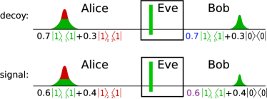
For a given decoy single-photon yield $Y_{1}^{(\mathrm{d})}$, we denote the smallest possible value Eve can achieve for $Y_{1}^{(\mathrm{s})}$ as $Y_{1,\mathrm{lb}}^{(\mathrm{s})}\big{(}Y_{1}^{(\mathrm{d})}\big{)}$. In our example above, we have $Y_{1,\mathrm{lb}}^{(\mathrm{s})}=6/7\cdot Y_{1}^{(\mathrm{d})}$ for $Y_{1}^{(\mathrm{d})}\leq 0.7$, because in this case the photons of the first mode are sufficient to reach $Y_{1}^{(\mathrm{d})}$. Thus Eve can completely block the second mode and let only photons of the first mode pass. For $Y_{1}^{(\mathrm{d})}>0.7$, Eve additionally has to let a fraction $(Y_{1}^{(\mathrm{d})}-0.7)/0.3$ of the photons in the second mode pass to reach $Y_{1}^{(\mathrm{d})}$, resulting in $Y_{1,\mathrm{lb}}^{(\mathrm{s})}=0.6+(Y_{1}^{(\mathrm{d})}-0.7)/0.3\cdot 0.4$.

This concept is easily extended to all $N$ modes that contribute to the state of Equation (13). Without loss of generality, we take $m_{1}^{(\mathrm{d})}/m_{1}^{(\mathrm{s})}\geq m_{2}^{(\mathrm{d})}/m_{2}^{(\mathrm{s})}\geq\ldots\geq m_{N}^{(\mathrm{d})}/m_{N}^{(\mathrm{s})}$. Only letting photons from the first mode pass results in the smallest ratio between $Y_{1}^{(\mathrm{s})}$ and $Y_{1}^{(\mathrm{d})}$, but this is only possible if $Y_{1}^{(\mathrm{d})}\leq m_{1}^{(\mathrm{d})}$. Otherwise, additional photons from other modes are needed to achieve the desired $Y_{1}^{(\mathrm{d})}$. The number $K$ of required modes is implicitly defined by

$$\sum_{k=1}^{K-1}m_{k}^{(\mathrm{d})}\leq Y_{1}^{(\mathrm{d})}<\sum_{k=1}^{K}m_{k}^{(\mathrm{d})},$$ (16)

such that both inequalities hold. Eve can achieve the lowest possible value for $Y_{1}^{(\mathrm{s})}$ by letting all photons of the first $K-1$ modes, and a fraction $\left(Y_{1}^{(\mathrm{d})}-\sum_{k=1}^{K-1}m_{k}^{(\mathrm{d})}\right)/m_{K}^{(\mathrm{d})}$ of the photons in the $K$th mode pass. This gives the desired value for the decoy single-photon yield

$$Y_{1}^{(\mathrm{d})}=\sum_{k=1}^{K-1}m_{k}^{(\mathrm{d})}+\frac{Y_{1}^{(\mathrm{d})}-\sum_{k=1}^{K-1}m_{k}^{(\mathrm{d})}}{m_{K}^{(\mathrm{d})}}m_{K}^{(\mathrm{d})},$$ (17)

and the lower bound

$$Y_{1,\mathrm{lb}}^{(\mathrm{s})}\left(Y_{1}^{(\mathrm{d})}\right)=\sum_{k=1}^{K-1}m_{k}^{(\mathrm{s})}+\frac{Y_{1}^{(\mathrm{d})}-\sum_{k=1}^{K-1}m_{k}^{(\mathrm{d})}}{m_{K}^{(\mathrm{d})}}m_{K}^{(\mathrm{s})}$$ (18)

for the signal single-photon yield for a given $Y_{1}^{(\mathrm{d})}$.

Step 2 - Upper bound on $Y_{\mathrm{M}}^{(\mathrm{d})}$ for a given $Y_{\mathrm{M}}^{(\mathrm{s})}$: In this step, we want to find the highest possible decoy multiphoton yield that is compatible with a given signal multiphoton yield. With minor modifications, this works out analogously to step 1, the only difference being that we have to keep track of all possible distributions of the photons among the modes. For this purpose, we introduce the set $Q=\{\mathbf{l}\in\mathbb{N}_{0}^{N}|\sum_{k=1}^{N}l_{k}\geq 2\}$. Each member of this set represents a multiphoton event with $l_{i}$ photons in the $i$th mode.

Similarly to $m_{k}$ for the single-photon case, we define $h_{\mathbf{l}}$ as the probability that a multiphoton event possesses the photon distribution specified by $\mathbf{l}\in Q$. It is given by

$$h_{\mathbf{l}}^{(\mathrm{s/d})}=\frac{1}{P_{\mathrm{M}}^{(\mathrm{s/d})}}\prod_{k=1}^{N}p^{(\mathrm{s/d})}(k,l_{k})$$ (19)

with the multiphoton probability

$$P_{\mathrm{M}}^{(\mathrm{s/d})}=\sum_{n\geq 2}P_{2}^{(\mathrm{s/d})}=1-P_{0}^{(\mathrm{s/d})}-P_{1}^{(\mathrm{s/d})},$$ (20)

where $P_{n}^{(\mathrm{s/d})}$ denotes the convoluted photon number distribution of all modes. Accordingly, $P_{0}^{(\mathrm{s/d})}=\prod_{k=1}^{N}p^{(\mathrm{s/d})}(k,0)$ and $P_{1}^{(\mathrm{s/d})}$ is given by Equation (15). Employing the mode distribution probabilities of Equation (19), the states of Equation (12) conditioned on a multiphoton event can be written as

$$\rho_{\mathrm{M}}^{(\mathrm{s/d})}=\sum_{\mathbf{l}\in Q}h_{\mathbf{l}}^{(\mathrm{s/d})}\bigotimes_{k=1}^{N}\ket{l_{k};\xi_{k}}\bra{l_{k};\xi_{k}}.$$ (21)

Again, Eve is not only allowed to make a photon number measurement but can also determine the mode distribution $\mathbf{l}$ of a multiphoton event. Thus she can selectively block multiphoton events with certain mode distributions. The highest possible $Y_{\mathrm{M}}^{(\mathrm{d})}$ for a given $Y_{\mathrm{M}}^{(\mathrm{s})}$ is achieved if Eve lets only events with the highest ratio between $h_{\mathbf{l}}^{(\mathrm{d})}$ and $h_{\mathbf{l}}^{(\mathrm{s})}$ pass. To sort the mode distributions accordingly, we define $L_{1}=\operatorname*{argmax}_{L\in Q}h_{L}^{(\mathrm{d})}/h_{L}^{(\mathrm{s})}$ and recursively

$$L_{i}=\operatorname*{argmax}_{L\in Q\setminus\{L_{1},\ldots,L_{i-1}\}}\frac{h_{L}^{(\mathrm{d})}}{h_{L}^{(\mathrm{s})}}\qquad\text{for }i\geq 2.$$ (22)

With that definition, we can apply the same method as in step 1. For a given $Y_{\mathrm{M}}^{(\mathrm{s})}$, we define $K$ implicitly by

$$\sum_{i=1}^{K-1}h_{L_{i}}^{(\mathrm{s})}\leq Y_{\mathrm{M}}^{(\mathrm{s})}<\sum_{i=1}^{K}h_{L_{i}}^{(\mathrm{s})}.$$ (23)

The highest possible $Y_{\mathrm{M}}^{(\mathrm{d})}$, compatible with a given $Y_{\mathrm{M}}^{(\mathrm{s})}$, is achieved if all multiphoton events with mode distributions $L_{1}$ to $L_{K-1}$, and the remaining fraction $\left(Y_{\mathrm{M}}^{(\mathrm{s})}-\sum_{i=1}^{K-1}h_{L_{i}}^{(\mathrm{s})}\right)/h_{L_{K}}$ with mode distribution $L_{K}$ are transmitted to Bob’s side. As a result we have the upper bound

$$Y_{\mathrm{M,ub}}^{(\mathrm{d})}(Y_{\mathrm{M}}^{(\mathrm{s})}) =\sum_{i=1}^{K-1}h_{L_{i}}^{(\mathrm{d})}+\frac{Y_{\mathrm{M}}^{(\mathrm{s})}-\sum_{i=1}^{K-1}h_{L_{i}}^{(\mathrm{s})}}{h_{L_{K}}^{(\mathrm{s})}}h_{L_{K}}^{(\mathrm{d})}$$ (24)

on the decoy multiphoton yield $Y_{\mathrm{M}}^{(\mathrm{d})}$ for a given signal multiphoton yield $Y_{\mathrm{M}}^{(\mathrm{s})}$.

Step 3 - The new bound on $Y_{1}^{(\mathrm{s})}$ for given gains $Q^{(\mathrm{s})}$ and $Q^{(\mathrm{d})}$: With the derived relations between the yields of signal and idler events, we are now able to calculate a new lower bound on $Y_{1}^{(\mathrm{s})}$ for given signal and decoy gains. If the relations were just given by a constant ratio, this would be in direct analogy to the single-mode case where the ratio of signal and decoy yields was fixed. This means we could plug the relations into Equation (4) and solve Equations (2) and (4) for a lower bound on $Y_{1}^{(\mathrm{s})}$. However, the derived relations, Equations (18) and (24), do not have a simple functional form. Hence an iterative approach is required to determine the new lower bound on $Y_{1}^{(\mathrm{s})}$.

We first solve Equations (2) and (4) for $Y_{\mathrm{M}}^{(\mathrm{s})}$ and $Y_{1}^{(\mathrm{d})}$, respectively:

$$Y_{\mathrm{M}}^{(\mathrm{s})} =\frac{1}{P_{\mathrm{M}}^{(\mathrm{s})}}\left[Q^{(\mathrm{s})}-P_{0}^{(\mathrm{s})}Y_{0}-P_{1}^{(\mathrm{s})}Y_{1}^{(\mathrm{s})}\right],$$ (25)

$$Y_{1}^{(\mathrm{d})} =\frac{1}{P_{1}^{(\mathrm{d})}}\left[Q^{(\mathrm{d})}-P_{0}^{(\mathrm{d})}Y_{0}-P_{\mathrm{M}}^{(\mathrm{d})}Y_{\mathrm{M}}^{(\mathrm{d})}\right].$$ (26)

Alice and Bob know $Y_{0}$ from the vacuum decoy state. They can measure $Q^{(\mathrm{s})}$ and $Q^{(\mathrm{d})}$, and they know $P_{0}$, $P_{1}$ and $P_{M}$ for both signal and decoy because they know the properties of their source. In addition, a trivial lower bound on $Y_{1}^{(\mathrm{s})}$ is given by $Y_{1}^{(\mathrm{s})}\geq Y_{1,\mathrm{LB}}^{(\mathrm{s})}=0$. Starting with that value, a tighter bound can be calculated by the following algorithm:

1. Start by calculating an upper bound on $Y_{\mathrm{M}}^{(\mathrm{s})}$ from $Y_{1,\mathrm{LB}}^{(\mathrm{s})}$, using Equation (25):

   $$Y_{\mathrm{M,UB}}^{(\mathrm{s})}=\frac{1}{P_{\mathrm{M}}^{(\mathrm{s})}}\left[Q^{(\mathrm{s})}-P_{0}^{(\mathrm{s})}Y_{0}-P_{1}^{(\mathrm{s})}Y_{1,\mathrm{LB}}^{(\mathrm{s})}\right]$$ (27)

2. Next, use $Y_{\mathrm{M,UB}}^{(\mathrm{s})}$ to derive an upper bound on $Y_{\mathrm{M}}^{(\mathrm{d})}$ with Equation (24)

   $$Y_{\mathrm{M,UB}}^{(\mathrm{d})}=Y_{\mathrm{M,ub}}^{(\mathrm{d})}\left(Y_{\mathrm{M,UB}}^{(\mathrm{s})}\right)$$ (28)

3. Obtain a lower bound on $Y_{1}^{(\mathrm{d})}$ from $Y_{\mathrm{M,UB}}^{(\mathrm{d})}$ with Equation (26):

   $$Y_{1,\mathrm{LB}}^{(\mathrm{d})}=\frac{1}{P_{1}^{(\mathrm{d})}}\left[Q^{(\mathrm{d})}-P_{0}^{(\mathrm{d})}Y_{0}-P_{\mathrm{M}}^{(\mathrm{d})}Y_{\mathrm{M,UB}}^{(\mathrm{d})}\right]$$ (29)

4. Finally, determine a lower bound on $Y_{1}^{(\mathrm{s})}$ from $Y_{1,\mathrm{LB}}^{(\mathrm{d})}$, using Equation (18)

   $$Y_{1,\mathrm{LB}}^{(\mathrm{s})}=Y_{1,\mathrm{lb}}^{(\mathrm{s})}\left(Y_{1,\mathrm{LB}}^{(\mathrm{d})}\right)$$ (30)

The value obtained in Equation (30) can iteratively be plugged into the previously described steps as initial value, which results in an even tighter bound. After each iteration step, the final value for $Y_{1,\mathrm{LB}}^{(\mathrm{s})}$ is at least as large as the starting value, so the iteratively obtained values are monotonically increasing. As $Y_{1,\mathrm{LB}}^{(\mathrm{s})}\leq 1$ is bounded from above (not more than 100% of the events can result in a click of Bob’s detector), the series converges, giving the final lower bound on the single-photon yield of the signal state.

V New Bound on $e_{1}^{(\mathrm{s})}$

We also need to bound the error rate of the single-photon events of the signal state from above. In this case, Eve wants to introduce as many errors as possible into the single-photon events of the signal state while leaving the measured QBERs as expected, because this way she can gain the maximal amount of information from the signal single-photon events. An upper bound on the decoy single-photon events is given by Equation (7) if we use $Y_{1,\mathrm{LB}}^{(\mathrm{d})}$ given by the value (29) obtained in the iteration for determining $Y_{1,\mathrm{LB}}^{(\mathrm{s})}$. Since the errors also have to be assumed to be under Eve’s control, she is free to choose the modes into which the errors occur. The highest error rate of the signal single-photon events compared to the error rate of the decoy single-photon events is obtained if the errors are introduced into modes with a large $m_{k}^{(\mathrm{s})}/m_{k}^{(\mathrm{d})}$ ratio. Hence, if we again define K implicitly by

$$\sum_{\mathchoice{\hbox to0.0pt{\hss$\displaystyle{k=K}$\hss}}{\hbox to0.0pt{\hss$\textstyle{k=K}$\hss}}{\hbox to0.0pt{\hss$\scriptstyle{k=K}$\hss}}{\hbox to0.0pt{\hss$\scriptscriptstyle{k=K}$\hss}}}^{N}m_{k}^{(\mathrm{d})}\leq e_{1,\mathrm{ub}}^{(\mathrm{d})}<\sum_{i=K-1}^{N}m_{k}^{(\mathrm{d})},$$ (31)

the worst case assumption is that all photons in modes $N,N-1,\ldots,K$ and a fraction $\left(e_{1,\mathrm{ub}}^{(\mathrm{d})}-\sum_{k=K}^{N}m_{k}^{(\mathrm{d})}\right)/m_{K-1}^{(\mathrm{d})}$ of the photons in mode $K-1$ are erroneous. This gives the new upper bound on the signal single-photon error rate,

$$e_{1,\mathrm{ub}}^{(\mathrm{s})}=\sum_{\mathchoice{\hbox to0.0pt{\hss$\displaystyle{k=K}$\hss}}{\hbox to0.0pt{\hss$\textstyle{k=K}$\hss}}{\hbox to0.0pt{\hss$\scriptstyle{k=K}$\hss}}{\hbox to0.0pt{\hss$\scriptscriptstyle{k=K}$\hss}}}^{N}m_{k}^{(\mathrm{s})}+\frac{e_{1,\mathrm{ub}}^{(\mathrm{d})}-\sum_{k=K}^{N}m_{k}^{(\mathrm{d})}}{m_{K-1}^{(\mathrm{d})}}m_{K-1}^{(\mathrm{s})}.$$ (32)

VI Numerical Simulations

With the new lower bound on $Y_{1}^{(\mathrm{s})}$, obtained by Equation (30) in the iteration, and the new upper bound on $e_{1}^{(\mathrm{s})}$ given by Equation (32), we can determine a lower bound on the achievable key rate for states of the form (12) with Equation (1).

In the following simulations, we consider the simplest example for the use of a PDC source in a QKD protocol. Signal and decoy states are created with different pump intensities, and only the photons in the signal mode are used for information encoding, while the photons in the idler mode are ignored. The PDC output state is modeled with a full multimode structure and is given by Equation (9), resulting in the state (12) after tracing over the idler mode. The photon number distribution for each spectral mode is given by

$$p^{(\mathrm{s/d})}(k,n)=\operatorname{sech}^{2}r_{k}^{(\mathrm{s/d})}\tanh^{2n}r_{k}^{(\mathrm{s/d})},$$ (33)

with $r_{k}^{(\mathrm{s/d})}\propto\lambda_{k}\sqrt{I^{(\mathrm{s/d})}}$ describing the corresponding squeezing parameters. $I^{(\mathrm{s})}$ and $I^{(\mathrm{d})}$ are the pump intensities for signal and decoy state, respectively, and $\lambda_{k}$ indicates how prominent the $k$th mode is. The coefficients $\lambda_{k}$ are properties of the PDC crystal and the pump.

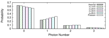
The photon number distribution for each spectral mode, Equation (33), is a thermal distribution. Thus the single-mode case ($\lambda_{k}=\delta_{k1}$) corresponds to thermal photon number distribution. With more contributing modes, the distribution is changed from thermal towards a Poissonian distribution. This is shown in Figure 2 for the values of Table 1 and a mean photon number of 0.6.

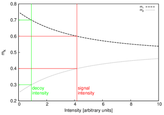
Let us first illustrate, by means of a simple example, how different mode occupation probabilities arise for signal and decoy state. Consider a PDC state with just two spectral modes that have $\lambda_{1}=\sqrt{0.75}$ and $\lambda_{2}=\sqrt{0.25}$. The mode occupation probabilities for a single-photon event are then given by

$$m_{1}(I) =\frac{p(1,1)p(2,0)}{p(1,1)p(2,0)+p(1,0)p(2,1)}$$

$$=\frac{\tanh^{2}r_{1}}{\tanh^{2}r_{1}+\tanh^{2}r_{2}},$$ (34)

$$m_{2}(I) =\frac{\tanh^{2}r_{2}}{\tanh^{2}r_{1}+\tanh^{2}r_{2}}.$$ (35)

They inherit the intensity dependence from the squeezing parameters $r_{1}$ and $r_{2}$. This intensity dependence is shown in Figure 3, along with chosen decoy and signal intensities such that we end up exactly with the states shown in Figure 1.

Now, we focus on a physically realistic case. Our source is a waveguided periodically poled KTP crystal with a grating period of $\Lambda=68.40\mu$m, length of 5 mm, and waveguide width and height both 4 $\mu$m. The pump laser spectrum is centered at a wavelength of 775nm and the signal and idler are frequency degenerate around 1550nm. We study four different pump bandwidths $\sigma$, which lead to different values for $\lambda_{k}$ Mauerer2008 . They are shown in Table 1.

Width $\sigma$	$\lambda_{k}$
1 nm	0.959, 0.194, 0.152, 0.098, 0.088, 0.033, 0.032, 0.014
2 nm	0.871, 0.463, 0.140, 0.064, 0.054, 0.028, 0.001
4 nm	0.690, 0.555, 0.383, 0.222, 0.107, 0.054, 0.050, 0.044,
	0.023, 0.012, 0.004, 0.003, 0.001
8 nm	0.511, 0.478, 0.427, 0.364, 0.296, 0.228, 0.167, 0.117,
	0.078, 0.056, 0.047, 0.037, 0.023, 0.015, 0.014, 0.011,
	0.006, 0.003, 0.001

Table 1: $\lambda_{k}$ for the KTP crystal for different pump widths.

Figure 2: (Color online) The photon number distributions for different pump widths $\sigma$.

Figure 3: (Color online) The mode occupation probabilities $m_{1}$ and $m_{2}$ for a single-photon event in dependence of the pump intensity.

We first consider the case of $\sigma=4$nm. For given pump intensities for signal and decoy state, the mode occupation probabilities can be calculated with Equations (14) and (19) for the single-photon and multiphoton state, respectively. We assume that Eve designs her attack such that her presence cannot be detected. This implies that the measured gains and error rates for signal and decoy state have the values that are expected from natural losses and detection errors. According to Lo2005 , they are given by

$$Q^{(\mathrm{s/d})}=\sum_{n}Y_{n}P_{n}^{(\mathrm{s/d})},$$ (36)

$$E^{(\mathrm{s/d})}=\frac{1}{Q^{(\mathrm{s/d})}}\sum_{n}e_{n}Y_{n}P_{n}^{(\mathrm{s/d})},$$ (37)

with the overall (i.e., convoluted) photon number distributions $P_{n}^{(\mathrm{s/d})}$ and

$$Y_{n}\approx\eta_{n}+p_{\textrm{dark}},$$ (38)

$$e_{n}=\frac{1}{Y_{n}}\left(e_{\textrm{det}}\eta_{n}+\frac{1}{2}p_{\textrm{dark}}\right).$$ (39)

In these equations, $p_{\textrm{dark}}$ is the dark count probability of Bob’s detector, $e_{\textrm{det}}$ is the detection error (i.e., the probability that Alice prepares a 0 (1), but Bob detects a 1 (0)), and $\eta_{n}=1-(1-\eta)^{n}$ is the probability that at least one of $n$ photons arrives at Bob’s side and is detected. The overall detection probability $\eta=10^{-\alpha/10}\cdot\eta_{\mathrm{det}}$ of each photon is determined by the channel attenuation $\alpha$ in dB and the detector efficiency $\eta_{\mathrm{det}}$. We use the experimental parameters of Ref. Gobby2004 in the simulations, which are shown in Table 2.

Dark count probability	$1.7\cdot 10^{-6}$
Detection error	3.3%
Detector efficiency	4.5%

Table 2: Characteristics of Bob’s detector.

With the gains and QBER for signal and decoy states, Equations (38) and (39), a lower bound on the signal single-photon yield $Y_{1}^{(\mathrm{s})}$, and an upper bound on the signal single-photon error rate $e_{1}^{(\mathrm{s})}$ can be calculated as described in Sections IV and V. This allows us to compute a lower bound on the achievable key rate according to Equation (1). We compare this key rate to the key rate for a single-mode source with the same photon number distribution. In other words, the secure key rate one would falsely expect to be achievable if the multi-mode structure of the PDC state is ignored. It is calculated by Equation (1) with the bounds on $Y_{1}^{(\mathrm{s})}$ and $e_{1}^{(\mathrm{s})}$ given by Equations (5) and (7). The corresponding key rates are both plotted in Figure 4 against the channel attenuation. We find that the key rate drops about 10% when Eve’s new possible attack is taken into account by adjusting the bounds on $Y_{1}^{(\mathrm{s})}$ and $e_{1}^{(\mathrm{s})}$ accordingly. In both scenarios, the mean photon number of the decoy state is 0.1, and the mean photon number of the signal state is optimized to give the highest key rate.

Figure 4: (Color online) Solid (red) line: Lower bound on the secure key rate for the KTP crystal with a pump width of 4 nm. Dashed (green) line: Lower bound on secure key rate for the same photon number distribution, but with all photons in the same spectral mode. The inset shows a zoom of the 50-55km region. The weak decoy mean photon number is 0.1 in both cases, and the signal mean photon number is optimized to result in the largest possible rate.

Figure 5: (Color online) Lower bound on the secure key rate for different pump width and therefore different mode contributions. The asymptotic cases are the rates for thermal and Poissonian distribution. The inset shows the optimized mean photon number of the signal state. The weak decoy mean photon number is fixed to 0.1 for all scenarios.

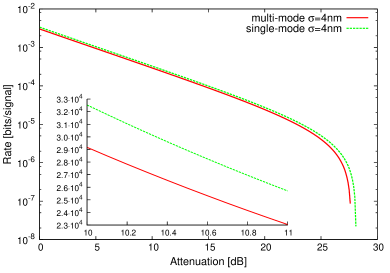
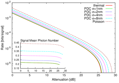
Figure 5 shows the secure key rate for all different pump widths given in Table 1. One can see that the secure key rate is higher when more modes contribute to the PDC process. This effect is explained by the change in the photon number distribution. With more contributing modes, the photon number distribution is shifted from a thermal distribution to a Poissonian distribution (see Figure 2). The Poissonian distribution is favorable in comparison to the thermal distribution, because the ratio between single-photon and multiphoton events increases. This permits a higher mean photon number for the signal state, which in turn increases the achievable key rate and distance. The resulting optimal mean photon numbers in dependence of the channel attenuation are depicted in the inset of Figure 5.

VII Conclusion

In summary, we have pointed out the necessity to carefully pay attention to the output states of the utilized sources, but likewise demonstrated that the demand for perfect indistinguishability of the signal and decoy photons, which is hard to implement in practice, can be loosened for only a small cost in the key rate.

The analysis was applied to a parametric down conversion (PDC) source, where the weak decoy state is created by pumping the crystal with a lower pump intensity. For about ten effectively contributing modes, we observed a drop of the key rate to roughly 90% of the corresponding value in the single-mode case with the same photon number distribution. The simulation was performed for different numbers of effectively contributing modes, leading to the conclusion that the advantageous change in the photon number distribution, which occurs if more modes contribute has a higher effect on the key rate than the aforementioned decrease due to the new attack possibility presented to Eve by the multi-mode structure of the states.

This analysis can also be used for a heralded PDC source, as long as the heralding detector is frequency independent, as the resulting states are also of the form of Equation (12). For heralding with a frequency dependent detector, the analysis has to be extended to the case where the density matrices for signal and decoy state are diagonal in different bases, contrary to our condition given by Equation (12).

Another possibility to produce the decoy state is by passive decoy generation Mauerer2007 ; Adachi2007 . In this scheme, the complications that arise because of the multi-mode structure of the PDC state can be avoided if a frequency independent detector is available for the decoy generation, as the spectral properties of $n$-photon states would then be the same for signal and decoy state. This, however, is not the case for a frequency dependent detector, because such a detector leads to signal and decoy states with different spectral properties. Again, the resulting states require an analysis for signal and decoy states that are diagonal in different bases.

We believe that this paper is a first step towards allowing more general signal and decoy states, which will significantly simplify the design of QKD sources.

References

- (1) C. H. Bennett and G. Brassard, in Proc. IEEE Int. Conf. on Computers, Systems, and Signal Processing (IEEE, New York, ADDRESS, 1984), pp. 175–179.
- (2) N. Gisin, G. Ribordy, W. Tittel, and H. Zbinden, Rev. Mod. Phys. 74, 145 (2002).
- (3) M. Dušek, N. Lütkenhaus, and M. Hendrych, Progress in Optics 49, 381 (2006).
- (4) W. Mauerer, W. Helwig, and C. Silberhorn, Ann. Phys. (Leipzig) 17, No. 2-3 158, 175 (2008).
- (5) D. Mayers, Journal of the ACM 3, 35 (1998).
- (6) P. W. Shor and J. Preskill, Phys. Rev. Lett. 85, 441 (2000).
- (7) D. Gottesman, H.-K. Lo, N. Lütkenhaus, and J. Preskill, Quant. Inf. Comp. 5, 325 (2004).
- (8) N. Lütkenhaus, Phys. Rev. A 61, 052304 (2000).
- (9) G. Brassard, N. Lütkenhaus, T. Mor, and B. C. Sanders, Phys. Rev. Lett. 85, 1330 (2000).
- (10) N. Lütkenhaus and M. Jahma, New J. Phys. 4, 44.1 (2002).
- (11) W.-Y. Hwang, Phys. Rev. Lett. 91, 057901 (2003).
- (12) H.-K. Lo, X. Ma, and K. Chen, Phys. Rev. Lett. 94, 230504 (2005).
- (13) X.-B. Wang, Phys. Rev. Lett. 94, 230503 (2005).
- (14) X. Ma, B. Qi, Y. Zhao, and H.-K. Lo, Phys. Rev. A 72, 012326 (2005).
- (15) W. Mauerer, M. Avenhaus, W. Helwig, and C. Silberhorn, arXiv:0812.3597v1 (2008).
- (16) W. K. Wootters and W. H. Zurek, Nature 299, 802 (1982).
- (17) P. J. Mosley et al., Physical Review Letters 100, 133601 (2008).
- (18) P. P. Rohde, W. Mauerer, and C. Silberhorn, New Journal of Physics 9, 91 (2007).
- (19) D. Gobby, Z. Yuan, and A. Shields, Appl. Phys. Lett. 84, 19 (2004).
- (20) W. Mauerer and C. Silberhorn, Phys. Rev. A 75, 050305 (R) (2007).
- (21) Y. Adachi, T. Yamamoto, M. Koashi, and N. Imoto, Phys. Rev. Lett. 99, 180503 (2007).