Néel Order and Electron Spectral Functions in the Two-Dimensional Hubbard Model:
a Spin-Charge Rotating Frame Approach

Abstract

Using recently developed quantum SU(2)$\times$ U(1) rotor approach, that provides a self-consistent treatment of the antiferromagnetic state we have performed electronic spectral function calculations for the Hubbard model on the square lattice. The collective variables for charge and spin are isolated in the form of the space-time fluctuating U(1) phase field and rotating spin quantization axis governed by the SU(2) symmetry, respectively. As a result interacting electrons appear as composite objects consisting of bare fermions with attached U(1) and SU(2) gauge fields. This allows us to write the fermion Green’s function in the space-time domain as the product CP¹ propagator resulting from the SU(2) gauge fields, U(1) phase propagator and the pseudo-fermion correlation function. As a result the problem of calculating the spectral line shapes now becomes one of performing the convolution of spin, charge and pseudo-fermion Green’s functions. The collective spin and charge fluctuations are governed by the effective actions that are derived from the Hubbard model for any value of the Coulomb interaction. The emergence of a sharp peak in the electron spectral function in the antiferromagnetic state indicates the decay of the electron into separate spin and charge carrying particle excitations.

I Introduction

Recent high-resolution angle-resolved photoemission spectroscopy (ARPES) studies revealed a complicated character of electronic structure and quasiparticle (QP) spectra in copper oxide superconductors.arpes In the discussion of photoemission on solids, and in particular on the correlated electron systems, the most powerful and commonly used approach is based on the Green’s–function formalism. In this context, the propagation of a single electron in a many-body system is described by the time-ordered one-electron Green’s propagator. A common approach in describing strong electron correlations is based on consideration of the Hubbard model.hubbard It allows to study a moderate correlation limit observed experimentally in cuprates and more consistently takes into account subtleties of the electronic structure, in particular, a spectral weight transfer.meind In qualitative sense the Hubbard model serves as the standard model of correlated electron systems, and has the same conceptional importance for interacting electrons as the Ising model for classical statistical mechanics. Here, the low number of explicit parameters provides the ideal condition for a thorough test of the power and quality of analytical and numerical methods. As a matter of fact intensive studies on this model have revealed subtlety of the results and controversies depending on approaches, and approximations. The two-dimensional (2D) Hubbard model was studied in Ref. zlatic, . The single particle self-energy was calculated by perturbation theory with the strength of the local Coulomb interaction as the expansion parameter to the second order. The main effect of correlations is the transfer of the spectral weight to the high energies. The 2D Hubbard model on the square lattice was also studied in the presence of lattice distortions in the adiabatic approximation.lamas In the absence of distortions the weight of the logarithmic singularity which characterizes the free system is reduced. Large $U$ values give rise to the typical two-peaks situation corresponding to the infinite $U$ limit. In other works, the 2D Hubbard model was considered with the quantum Monte Carlo method,monte1 ; monte2 ; monte3 recently also in the dynamical cluster approach.vidhya To solve the cluster problem the Hirsch-Fye quantum Monte Carlo method has been combined with the maximum entropy method to calculate the real frequency spectra. The effect of larger clusters and interactions was also explored however, these results were restricted by computational limitations including, especially, the minus sign problem.juillet1 Method based on numerical simulations for finite clusters precludes, however, to study subtle features of QP spectra due to poor energy and wave-vector resolutions in small size clusters.bulut Thus careful analyzes of finite-size effects are important in numerical studies, especially for low-energy excitations. In the dynamical mean field theory (DMFT) the self-energy is treated in the single-site approximation which is unable to describe wave-vector dependent phenomena.dmft To overcome the difficulties present in DMFT, various types of the dynamical cluster theory were developed.cluster In these methods only a restricted wave-vector and energy resolutions can be achieved, depending on the size of the clusters, while the physical interpretation of the origin of an anomalous electronic structure in numerical methods is not straightforward. In the Two-Particle Self-Consistent (TPSC) approach,vilk1 ; vilk2 that is based on enforcing sum rules and conservation laws, rather than on diagrammatic perturbative methods, a Luttinger-Ward functional is parametrized by two irreducible vertices that are local in space-time. This generates random phase approximation-like (RPA) equations for spin and charge fluctuations. The approach has the simple physical appeal of RPA but it satisfies key constraints that are always violated by RPA, namely the Mermin-Wagner theorem and the Pauli principle. The inherent difficulty of dealing with Hamiltonians appropriate for strongly correlated electronic systems originates from the non-perturbative nature of the problem and the presence of several competing physical mechanisms. In the fermionic systems with spin and charge excitations, however, the situation is much more complicated because dynamic quantum fluctuations are important even in large dimensions. Moreover, short-range spatial correlations play a key role, in particular magnetic correlations, leading to a strong tendency towards the formation of singlet bonds, as well as pair correlations. These correlations deeply affect the nature of quasiparticles. A new approach may therefore be needed, and a necessary requirement for a theory aiming to capture the essential physics of electrons correlated systems might be the inclusion of the fundamental ingredients of the physics as the underlying spin and charge symmetries as well as the associated ordered states. In this context the spectral properties of the two dimensional systems with strong magnetic fluctuations were investigated within the spin-fermion modelchubukov in the quasistatic approach that neglects the effect of dynamic spin fluctuations. The latter approach yields the two-peak structure of the spectral function for the antiferromagnetic correlations.

The other completely different approaches rest on gauge theories that arise in models of strongly interacting electrons: it is often convenient to change variables from electron operators to other degrees of freedom that represents the intrinsic symmetries of the system under study. This route turns out to be beneficial since several quantum phases of matter (for instance a antiferromagnet or a superconductor) may be characterized in terms of the symmetries that are broken spontaneously in that state. borejsza1 ; dupuis1 We employ this idea in the present paper to perform the one-particle spectral function calculations for the Hubbard model on the square lattice using a recently developed the quantum SU(2)$\times$U(1) rotor approach.zal The collective variables for charge and spin are isolated in the form of the space–time fluctuating U(1) phase field and rotating spin quantization axis governed by the SU(2) symmetry, respectively. As a result interacting electrons appear as a composite objects consisting of bare fermions with attached U(1) and SU(2) gauge fields. This allows us to write the fermion Green’s function in the space-time domain as the product of the complex-projective (CP¹) propagator (which results from the SU(2) gauge fields), U(1) phase propagator and the pseudo-fermion correlation function. The problem of calculating the spectral line shapes now becomes one of calculating the convolution of spin, charge and pseudo-fermion Green’s functions. The collective spin and charge fluctuations are governed by the effective actions that are derived from the Hubbard model for any value of the Coulomb interaction. We show that the method is useful for explicit calculation of spectral properties, enabling systematic inclusion of fluctuations of the charge as well as of the variable spin quantization axis. We demonstrate that the emergence of a sharp peak in the electron spectral function in the antiferromagnetic state points to the electron decaying into separate spin and charge carrying particle excitations.

The paper is organized as follows. After introduction of the model Hamiltonian in Section II, we present in Sec. III the transformations to the phase and spin angular variables that reflect the basic symmetries of the Hubbard model. Section IV is devoted to the derivation of the effective actions that govern the behavior of the system in the charge, spin and pseudo-fermion sectors, respectively. The self-consistent equations for the effective parameters of the model that follows from the effective actions are summarized in Section V. Section VI is devoted to a detailed analysis of the electronic spectral functions. Conclusions and discussions are given in Section VII. A number of technical details that pertain to the derivation of spectral functions is relegated to the Appendices.

II The Model

A prototype of theoretical understanding of the physics of strongly correlated systems is achieved by using simplified lattice fermionic systems, in particular, the Hubbard model given by the Hamiltonian ${\cal H}\equiv{\cal H}_{t}+{\cal H}_{U}$:

$${\cal H}=-t\sum_{\langle{\bf r}{\bf r}^{\prime}\rangle,\alpha}[c_{\alpha}^{\dagger}({\bf r})c_{\alpha}({\bf r}^{\prime})+{\rm h.c.}]-\mu\sum_{{\bf r}}n({\bf r})+\mathcal{H}_{U},$$ (1)

where the Hubbard interaction term is given by

$$\mathcal{H}_{U}=U\sum_{{\bf r}}n_{\uparrow}({\bf r})n_{\downarrow}({\bf r})$$ (2)

and $n({\bf r})=n_{\uparrow}({\bf r})+n_{\downarrow}({\bf r})$ is the number operator. Here, $\langle{\bf r},{\bf r}^{\prime}\rangle$ runs over the nearest-neighbor (n.n.) sites, $t$ is the hopping amplitude, $U$ stands for the Coulomb repulsion, while the operator $c_{\alpha}^{\dagger}({\bf r})$ creates an electron with spin $\alpha=\uparrow(\equiv 1),\downarrow(\equiv 2)$ at the lattice site ${\bf r}$, where $n_{\alpha}({\bf r})=c_{\alpha}^{\dagger}({\bf r})c_{\alpha}({\bf r})$. The chemical potential $\mu$ controls the average number of electrons. The kinetic energy operator ${\cal H}_{t}$ reflects the electrons’ itinerant features while the interaction operator ${\cal H}_{U}$ forces the electrons’ correlated motion or even their localization.

Since the partition function often serves as a starting point for the calculation of thermodynamic properties, it is instructive to take a closer look at how this quantity may be obtained within the path integral formalism. To this end it is customary to introduce Grassmann fields, $c_{\alpha}({\bf r}\tau)$ depending on the “imaginary time” $0\leq\tau\leq\beta\equiv 1/k_{B}T$, (with $T$ being the temperature) that satisfy the anti–periodic condition $c_{\alpha}({\bf r}\tau)=-c_{\alpha}({\bf r}\tau+\beta)$, to write the path integral for the statistical sum

$${\cal Z}=\int\left[{\cal D}\bar{c}{\cal D}c\right]e^{-{\cal S}[\bar{c},c]}$$ (3)

with the fermionic action

$${\cal S}[\bar{c},c]={\cal S}_{B}[\bar{c},c]+\int_{0}^{\beta}d\tau{\cal H}[\bar{c},c],$$ (4)

which contains the fermionic Berry termberry

$${\cal S}_{B}[\bar{c},c]=\sum_{{\bf r}\alpha}\int_{0}^{\beta}d\tau\bar{c}_{\alpha}({\bf r}\tau)\partial_{\tau}c_{\alpha}({\bf r}\tau)$$ (5)

that will play an important role in our considerations.

III Spin-charge rotating reference frame

The spin-rotational symmetry present in the Hubbard Hamiltonian is instrumental for obtaining proper low energetic properties. Therefore, it is crucial to construct a theoretical formulation that naturally preserves this symmetry. In particular, one should consider the spin-quantization axis to be a priori arbitrary and integrate over all possible directions in the partition function. It can be achieved when the density–density product in Eq.(1) is written, following Ref. schulz, , in a spin-rotational invariant way:

$${\cal H}_{U}=U\sum_{{\bf r}}\left\{\frac{1}{4}n^{2}({\bf r}\tau)-\left[{\bf\Omega}({\bf r}\tau)\cdot{\bf S}({\bf r}\tau)\right]^{2}\right\},$$ (6)

where $S^{a}({\bf r}\tau)=\frac{1}{2}\sum_{\alpha\alpha^{\prime}}c_{\alpha}^{\dagger}({\bf r}\tau)\hat{\sigma}_{\alpha\alpha^{\prime}}^{a}c_{\alpha^{\prime}}({\bf r}\tau)$ denotes the vector spin operator ($a=x,y,z$) with $\hat{\sigma}^{a}$ being the Pauli matrices. The unit vector

$${\bf\Omega}({\bf r}\tau) = [\sin\vartheta({\bf r}\tau)\cos\varphi({\bf r}\tau),\sin\vartheta({\bf r}\tau)\sin\varphi({\bf r}\tau),$$ (7)

$$\cos\vartheta({\bf r}\tau)]$$

written in terms of polar angles labels varying in space-time spin quantization axis. The explicit spin–rotation invariance comes from the angular integration over ${\bf\Omega}({\bf r}\tau)$ at each site and time:

$${\cal Z}=\int[{\cal D}{\bf\Omega}]\int\left[{\cal D}\bar{c}{\cal D}c\right]e^{-{\cal S}[{\bf\Omega},\bar{c},c]},$$ (8)

where $[{\cal D}{\bf\Omega}]\equiv\prod_{{\bf r}\tau_{k}}\frac{\sin\vartheta({\bf r}\tau_{k})d\vartheta({\bf r}\tau_{k})d\varphi({\bf r}\tau_{k})}{4\pi}$ is the spin-angular integration measure.

III.1 Hubbard-Stratonovich decoupling

The spin and charge density terms of the Hamiltonian in Eq.(6) are of the fourth order in fermionic operators, so they must be decoupled using Hubbard-Stratonovich (HS) formulahs with the auxiliary fields $\varrho({\bf r}\tau)$ and $iV({\bf r}\tau)$ respectively. The partition function can be written in the formpopov

$${\cal Z} = \int[{\cal D}{\bf\Omega}]\int[{\cal D}V{\cal D}\varrho]\int\left[{\cal D}\bar{c}{\cal D}c\right]e^{-{\cal S}\left[{\bf\Omega},V,\varrho,\bar{c},c\right]}.$$ (9)

Consequently, the effective action reads:

$${\cal S}\left[{\bf\Omega},V,\varrho,\bar{c},c\right] = \sum_{{\bf r}}\int_{0}^{\beta}d\tau\left[\frac{\varrho^{2}({\bf r}\tau)}{U}+\frac{V^{2}({\bf r}\tau)}{U}\right.$$ (10)

$$+ \left.iV({\bf r}\tau)n({\bf r}\tau)+2\varrho({\bf r}\tau){\bf\Omega}({\bf r}\tau)\cdot{\bf S}({\bf r}\tau)\right]$$

$$+ {\cal S}_{B}[\bar{c},c]+\int_{0}^{\beta}d\tau{\cal H}_{t}[\bar{c},c].$$

Since, $U$ is the largest energy in the problem, the simple Hartree–Fock theory won’t work. To proceed, one has to isolate strongly fluctuating modes generated by the Hubbard term according to the charge U(1) and spin SU(2) symmetries.

III.2 U(1) charge frame

Now, we switch from the particle-number representation to the conjugate phase representation of the electronic degrees of freedom that is governed by the compact U(1) group. To this end the second quantized Hamiltonian of the model is translated to the phase representation with the help of the topologically constrained path integral formalism.schulman As a result the electrons emerge as composite particles consisting of of spin-carrying neutral fermions and topological charged bosons in a form of a flux tubes with the quantum phase variable dual to the local electron density. To this end we write the fluctuating “imaginary chemical potential” $iV({\bf r}\tau)$ as a sum of a static $V_{0}({\bf r})$ and periodic function

$$V({\bf r}\tau)=V_{0}({\bf r})+\tilde{V}({\bf r}\tau),$$ (11)

where, using Fourier series

$$\tilde{V}({\bf r}\tau)=\frac{1}{\beta}\sum_{n=1}^{\infty}[\tilde{V}({\bf r}\omega_{n})e^{i\omega_{n}\tau}+c.c.]$$ (12)

with $\omega_{n}=2\pi n/\beta$ ($n=0,\pm 1,\pm 2$) being the (Bose) Matsubara frequencies. Now, we introduce the U(1) phase field $\phi({\bf r}\tau)$ via the Faraday–type relationkopec

$$\dot{\phi}({\bf r}\tau)\equiv\frac{\partial\phi({\bf r}\tau)}{\partial\tau}=e^{-i\phi({\bf r}\tau)}\frac{1}{i}\frac{\partial}{\partial\tau}e^{i\phi({\bf r}\tau)}=\tilde{V}({\bf r}\tau).$$ (13)

Furthermore, by performing the local gauge transformation to the new fermionic variables $f_{\alpha}({\bf r}\tau)$:

$$\left[\begin{array}[]{c}c_{\alpha}({\bf r}\tau)\\ \bar{c}_{\alpha}({\bf r}\tau)\end{array}\right]=\left[\begin{array}[]{cc}z({\bf r}\tau)&0\\ 0&\bar{z}({\bf r}\tau)\end{array}\right]\left[\begin{array}[]{c}f_{\alpha}({\bf r}\tau)\\ \bar{f}_{\alpha}({\bf r}\tau)\end{array}\right],$$ (20)

where the unimodular parameter $|z({\bf r}\tau)|^{2}=1$ satisfies $z({\bf r}\tau)=e^{i\phi({\bf r}\tau)}$, we remove the imaginary term $i\int_{0}^{\beta}d\tau\tilde{V}({\bf r}\tau)n({\bf r}\tau)$ for all the Fourier modes of the $V({\bf r}\tau)$ field, except for the zero frequency. We point out here that a similar phase representation was developed in the context of Coulomb blockade in mesoscopic systems.schon

III.3 SU(2) spin frame

Subsequent SU(2) transformation from $f_{\alpha}({\bf r}\tau)$ to $h_{\alpha}({\bf r}\tau)$ operators,

$$\left[f_{\uparrow}({\bf r}\tau),\,\,\,f_{\downarrow}({\bf r}\tau)\right] = {\bf R}({\bf r}\tau)\left[\begin{array}[]{c}h_{\uparrow}({\bf r}\tau)\\ h_{\downarrow}({\bf r}\tau)\end{array}\right],$$ (23)

$${\bf R}({\bf r}\tau) \equiv \left[\begin{array}[]{cc}\zeta_{\uparrow}({\bf r}\tau)&-\bar{\zeta}_{\downarrow}({\bf r}\tau)\\ \zeta_{\downarrow}({\bf r}\tau)&\bar{\zeta}_{\uparrow}({\bf r}\tau)\end{array}\right]$$ (26)

with the constraint

$$|\zeta_{\uparrow}({\bf r}\tau)|^{2}+|\zeta_{\downarrow}({\bf r}\tau)|^{2}=1$$ (27)

takes away the rotational dependence on ${\bf\Omega}({\bf r}\tau)$ in the spin sector. This is done by means of the Hopf map fradkin

$${\bf R}({\bf r}\tau)\hat{\sigma}^{z}{\bf R}^{\dagger}({\bf r}\tau)=\hat{\sigma}\cdot{\bf\Omega}({\bf r}\tau)$$ (28)

that is based on the enlargement from two-sphere $S_{2}$ to the three-sphere $S_{3}\sim SU(2)$. The unimodular constraint in Eq.(27) can be resolved by using the parametrization

$$\zeta_{1\uparrow}({\bf r}\tau) = e^{-\frac{i}{2}[\varphi({\bf r}\tau)+\chi({\bf r}\tau)]}\cos\left[\frac{\vartheta({\bf r}\tau)}{2}\right]$$

$$\zeta_{\downarrow}({\bf r}\tau) = e^{\frac{i}{2}[\varphi({\bf r}\tau)-\chi({\bf r}\tau)]}\sin\left[\frac{\vartheta({\bf r}\tau)}{2}\right]$$ (29)

with the Euler angular variables $\varphi({\bf r}\tau),\,\vartheta({\bf r}\tau)$ and $\chi({\bf r}\tau)$, respectively. Here, the extra variable $\chi({\bf r}\tau)$ represents the U(1) gauge freedom of the theory as a consequence of $S_{2}\to S_{3}$ mapping. One can summarize Eqs (20) and (26) by the single joint gauge transformation exhibiting electron operator factorization

$$c_{\alpha}({\bf r}\tau) = \sum_{\alpha^{\prime}}\mathcal{U}_{\alpha\alpha^{\prime}}({\bf r}\tau)h_{\alpha^{\prime}}({\bf r}\tau),$$

$$\mathcal{U}({\bf r}\tau) = z({\bf r}\tau){\bf R}({\bf r}\tau),$$ (30)

where $\mathcal{U}\left(\mathbf{r}\tau\right)$ is a U(2) matrix which rotates the charge and spin-quantization axis at site ${\bf r}$ and time $\tau$. This reflects the composite nature of the interacting electron formed from bosonic spin and charge degrees of freedom given by ${R}_{\alpha\alpha^{\prime}}({\bf r}\tau)$ and $z({\bf r}\tau)$, respectively as well as remaining fermionic part $h_{\alpha}({\bf r}\tau)$. Accordingly, the integration measure over the group manifold becomes

$$\int[{\cal D}\phi{\cal D}{\bf\Omega}]\equiv\sum_{\{m({\bf r})\}}\prod_{{\bf r}}\int_{0}^{2\pi}d\phi_{0}({\bf r})\int d{\bf\Omega}_{0}({\bf r})$$

$$\times\int\limits_{{\bf\Omega}({\bf r}0)={\bf\Omega}_{0}}^{{\bf\Omega}({\bf r}\beta)={\bf\Omega}_{0}}{\cal D}{\bf\Omega}({\bf r}\tau)\int\limits_{\phi({\bf r}0)=\phi_{0}({\bf r})}^{\phi({\bf r}\beta)=\phi_{0}({\bf r})+2\pi m({\bf r})}{\cal D}\phi({\bf r}\tau),$$ (31)

where $\int d{\bf\Omega}\dots=\frac{1}{4\pi}\int_{0}^{\pi}\sin\theta d\vartheta\int_{0}^{2\pi}d\varphi\dots$ and $[{\cal D}{\bf\Omega}({\bf r}\tau)]=\prod_{k}d{\bf\Omega}({\bf r}\tau_{k})$. Here, $m\in{Z}$ labels equivalence classes of homotopically connected paths schulman for the U(1) group.

III.4 Solutions for $V_{0}({\bf r})$ and $\varrho({\bf r}\tau)$

Once can anticipate that spatial and temporal fluctuations of the fields $V_{0}({\bf r})$ and $\varrho({\bf r}\tau)$ will be energetically penalized, since they are linked to the high energy scale set by $U$ and decouple from the angular and phase variables. Therefore, in order to make further progress we next subject the corresponding functionals to a saddle point analysis. The expectation value of the static (zero frequency) part of the fluctuating potential $V_{0}(\mathbf{r})$ calculated by the saddle point method to give

$$V_{0}(\mathbf{r})=i\left(\mu-\frac{U}{2}n_{h}\right)\equiv i\bar{\mu},$$ (32)

where $\bar{\mu}$ is the chemical potential with a Hartree shift originating from the saddle-point value of the static variable $V_{0}({\bf r})$ with $n_{h}=n_{h\uparrow}+n_{h\downarrow}$ and $n_{h\alpha}=\langle\bar{h}_{\alpha}({\bf r}\tau)h_{\alpha}({\bf r}\tau)\rangle$. Similarly in the magnetic sector we have

$$\rho({\bf r}\tau)=(-1)^{{\bf r}}\Delta_{c},$$ (33)

where $\Delta_{c}=U\langle S^{z}({\bf r}\tau\rangle$ sets the magnitude for the Mott-charge gap. The solution delineated in Eq.(33) correspond to the saddle point of the antifferomagnetic type (with staggering $\Delta_{c}$) . Note that the notion “antifferomagnetic” here does not mean an actual long–range ordering - for this the angular spin-quantization variables ${\bf\Omega}({\bf r}\tau)$ have to be ordered as well. The mean-field parameter $\Delta_{c}$ has to be determined by the stationary points of the action, e.g., by the mean-field equations that will be derived more explicitly later on for our special purpose.

IV Effective actions

IV.1 Total fermionic phase-angular action

In the new variables the action in Eq.(10) assumes the form

$${\cal S}\left[{\bf\Omega},\phi,\varrho,\bar{h},h\right]={\cal S}_{B}[\bar{h},h]+\int_{0}^{\beta}d\tau{\cal H}_{{\bf\Omega,\phi}}[\rho,\bar{h},h]$$

$$\,\,\,\,\,+{\cal S}_{0}\left[\phi\right]+2\sum_{{\bf r}}\int_{0}^{\beta}d\tau{\bf A}({\bf r}\tau)\cdot{\bf S}_{h}({\bf r}\tau),$$ (34)

where

$${\bf S}_{h}({\bf r}\tau)=\frac{1}{2}\sum_{\alpha\gamma}\bar{h}_{\alpha}({\bf r}\tau)\hat{\sigma}_{\alpha\gamma}h_{\gamma}({\bf r}\tau).$$ (35)

Furthermore,

$$S_{0}[\phi]=\sum_{{\bf r}}\int_{0}^{\beta}d\tau\left[\frac{\dot{\phi}^{2}({\bf r}\tau)}{U}+\frac{1}{i}\frac{2\mu}{U}\dot{\phi}({\bf r}\tau)\right]$$ (36)

stands for the kinetic and Berry term of the U(1) phase field in the charge sector. The SU(2) gauge transformation in Eq.(26) and the fermionic Berry term generate SU(2) potentials given by

$${\bf R}^{\dagger}({\bf r}\tau)\partial_{\tau}{\bf R}({\bf r}\tau) = {\bf R}^{\dagger}\left(\dot{\varphi}\frac{\partial}{\partial\varphi}+\dot{\vartheta}\frac{\partial}{\partial\vartheta}+\dot{\chi}\frac{\partial}{\partial\chi}\right){\bf R}$$ (37)

$$= -\bm{\sigma}\cdot{\bf A}({\bf r}\tau),$$

where

$$A^{x}({\bf r}\tau) = \frac{i}{2}\dot{\vartheta}({\bf r}\tau)\sin\chi({\bf r}\tau)-\frac{i}{2}\dot{\varphi}({\bf r}\tau)\sin\theta({\bf r}\tau)\cos\chi({\bf r}\tau)$$

$$A^{y}({\bf r}\tau) = \frac{i}{2}\dot{\vartheta}({\bf r}\tau)\cos\chi({\bf r}\tau)+\frac{i}{2}\dot{\varphi}({\bf r}\tau)\sin\theta({\bf r}\tau)\sin\chi({\bf r}\tau)$$

$$A^{z}({\bf r}\tau) = \frac{i}{2}\dot{\varphi}({\bf r}\tau)\cos\vartheta({\bf r}\tau)+\frac{i}{2}\dot{\chi}({\bf r}\tau).$$ (38)

are the SU(2) gauge potentials. The fermionic sector, in turn, is governed by the effective Hamiltonian

$$\mathcal{H}_{\Omega,\phi}=\mathcal{H}_{\Omega,\phi}^{(\rho)}+\mathcal{H}_{\Omega,\phi}^{(t)},$$ (39)

where

$${\cal H}_{{\bf\Omega,\phi}}^{(\rho)} = \sum_{{\bf r}}(-1)^{{\bf r}}\Delta_{c}[\bar{h}_{\uparrow}({\bf r}\tau)h_{\uparrow}({\bf r}\tau)-\bar{h}_{\downarrow}({\bf r}\tau)h_{\downarrow}({\bf r}\tau)]$$

$${\cal H}_{{\bf\Omega,\phi}}^{(t)} = -t\sum_{\langle{\bf r},{\bf r}^{\prime}\rangle}\sum_{\alpha\gamma}\left[\mathcal{U}^{\dagger}({\bf r}\tau)\mathcal{U}({\bf r^{\prime}}\tau)\right]_{\alpha\gamma}\bar{h}_{\alpha}({\bf r}\tau)h_{\gamma}({\bf r}^{\prime}\tau)$$ (40)

$$- \bar{\mu}\sum_{{\bf r}\alpha}\bar{h}_{\alpha}({\bf r}\tau)h_{\alpha}({\bf r}\tau).$$

The result of the gauge transformations is that we have managed to cast the strongly correlated problem into a system of mutually non-interacting pseudo fermions, submerged in the bath of strongly fluctuating U(1) and SU(2) fields whose dynamics is governed by the energy scale set by the Coulomb interaction $U$ coupled to fermions via hopping term and with the Zeeman-type contribution with the massive field ${\varrho}({\bf r}\tau)$.

IV.2 Charge (phase) action

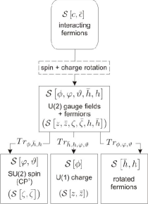
Figure 1: Scheme for the derivation of effective actions. The initial purely fermionic action of the Hubbard model is transformed into effective actions in spin, charge and fermionic sectors by performing the trace over selected set of variables.

In systems with Coulomb interactions, the phase variable dual to the charge is an important collective field. We start with a partition function for charge sector

$${\cal Z} = \int\left[{\cal D}\phi\right]e^{-\mathcal{S}[\phi]},$$ (41)

where the charge action requires tracing over fermionic and angular SU(2) variables

$$\mathcal{S}[\phi] = -\ln\int[{\cal D}\bar{h}{\cal D}h{\cal D}{\bf\Omega}]e^{-{\cal S}[\varphi,\phi,\vartheta,\bar{h},h]}.$$ (42)

To proceed, it is convenient to replace the phase degrees of freedom by the complex field

$$z\left(\mathbf{r}\tau\right) = e^{i\phi\left(\mathbf{r}\tau\right)}$$

$$\bar{z}\left(\mathbf{r}\tau\right) = e^{-i\phi\left(\mathbf{r}\tau\right)},$$ (43)

which satisfies the periodic boundary condition $z\left(\mathbf{r}\beta\right)=z\left(\mathbf{r}0\right)$. This can be done by implemented the Fadeev-Popov method with the Dirac delta functional resolution of the unity:kopec1

$$1\equiv\int\left[\mathcal{D}\bar{z}\mathcal{D}z\right]\delta\left[\frac{1}{N}\sum_{i}\left|z\left(\mathbf{r}\tau\right)\right|^{2}-1\right]$$

$$\times\prod_{i}\delta\left[z\left(\mathbf{r}\tau\right)-e^{i\phi\left(\mathbf{r}\tau\right)}\right]\delta\left[\bar{z}_{i}\left(\mathbf{r}\tau\right)-e^{-i\phi\left(\mathbf{r}\tau\right)}\right],$$ (44)

where we take $z\left(\mathbf{r}\tau\right)$ as continuous variable but constrained (on the average) to have the unimodular value. We can solve the constraint by introducing the Lagrange multiplier $\lambda$ which adds the quadratic terms (in the $z\left(\mathbf{r}\tau\right)$ fields) to the effective action. The partition function can be written in form

$$\mathcal{Z} = \int_{-i\infty}^{+i\infty}\left[\frac{{\cal D}\lambda_{z}}{2\pi i}\right]e^{-N\beta\mathcal{F}\left(\lambda_{z}\right)},$$ (45)

where the free energy per site $\mathcal{F}=-\ln\mathcal{Z}/\beta N$ is given by:

$$\mathcal{F} = -\lambda_{z}-\frac{1}{N\beta}\ln\int\left[\mathcal{D}\bar{z}\mathcal{D}z\right]e^{-{\cal S}_{\mathrm{eff}}[\bar{z},z]}$$

$${\cal S}_{\mathrm{eff}}[\bar{z},z] = \sum_{\langle\mathbf{r}\mathbf{r}^{\prime}\rangle}\int_{0}^{\beta}d\tau d\tau^{{}^{\prime}}\left[\lambda_{z}\delta_{\mathbf{r}\mathbf{r}^{\prime}}\delta\left(\tau-\tau^{\prime}\right)\right]$$ (46)

$$\left.-\mathcal{\gamma}\left(\mathbf{r}\tau,\mathbf{r}^{\prime}\tau^{\prime}\right)\right]\bar{z}(\mathbf{r}\tau)z(\mathbf{r}^{\prime}\tau^{\prime}),$$

where

$$\gamma\left(\mathbf{r}\tau,\mathbf{r}^{\prime}\tau^{\prime}\right)=\left\langle\exp\left\{-i\left[\phi\left(\mathbf{r}\tau\right)-\phi\left(\mathbf{r}^{\prime}\tau^{\prime}\right)\right]\right\}\right\rangle$$ (47)

is the two-point phase correlator associated with the order parameter field, where $\left\langle\dots\right\rangle$ is the averaging with respect to the action:

$$\mathcal{S}_{0}[\phi]=\sum_{{\bf r}}\int_{0}^{\beta}d\tau\left[\frac{\dot{\phi}^{2}({\bf r}\tau)}{U}+\frac{1}{i}\frac{2\mu}{U}\dot{\phi}({\bf r}\tau)\right].$$ (48)

The action with the topological contribution, after Fourier transform, we write as

$$\mathcal{S}_{\mathrm{eff}}[\bar{z},z]=\frac{1}{N\beta}\sum_{\mathbf{k},n}\bar{z}\left(\mathbf{k}\omega_{n}\right)\mathrm{G}_{z0\mathbf{k}}^{-1}\left(\omega_{n}\right)z\left(\mathbf{k}\omega_{n}\right),$$ (49)

where

$$\mathrm{G}_{z0\mathbf{k}}^{-1}\left(\omega_{n}\right)=\lambda_{z}+\gamma^{-1}\left(\omega_{n}\right)$$ (50)

is the inverse of the propagator, while the phase correlator after Fourier transform, can be written as as:

$$\gamma\left(\omega_{n}\right)=\frac{1}{\mathcal{Z}_{0}}\frac{4}{U}\sum_{m=-\infty}^{+\infty}\frac{e^{-\frac{\beta U}{2}\left(m+\frac{{\mu}}{U}\right)^{2}}}{1-4\left(m+\frac{{\mu}}{U}-\frac{i\omega_{n}}{U}\right)^{2}},$$ (51)

where

$$\mathcal{Z}_{0}=\sum_{m=-\infty}^{+\infty}\exp\left[-\frac{1}{2}\beta U\left(m+\frac{{\mu}}{U}\right)^{2}\right]$$ (52)

is the partition function for the set of non-interacting quantum rotors. Note that the presence of the integer winding numbers in Eqs (51) and (52) renders the phase propagator periodic in the reduced chemical potential $\mu/U$. The unimodular condition of the U(1) phase variables translates into the equation

$$1=\frac{1}{N\beta}\sum_{\mathbf{k},n}\frac{1}{\lambda_{z0}+\gamma^{-1}\left(\omega_{n}\right)},$$ (53)

which fixes the Lagrange multiplier $\lambda_{z0}$.

IV.3 Fermionic action

Now we turn to the effective action of pseudo–fermions by tracing out the gauge degrees of freedom. To this end we write the partition function as

$${\cal Z} = \int\left[{\cal D}\bar{h}{\cal D}{h}\right]e^{-{\cal S}[\bar{h},h]},$$ (54)

where

$${\cal S}[\bar{h},h] = -\ln\int[{\cal D}\phi{\cal D}{\bf\Omega}]e^{-{\cal S}[{\varphi,\phi,\vartheta},\bar{h},h]}$$ (55)

$$= \mathcal{S}_{B}[\bar{h},h]+{\cal S}_{t}^{(1)}[\bar{h},h]+{\cal S}_{t}^{(2)}[\bar{h},h]$$

$$+ \int_{0}^{\beta}d\tau{\cal H}_{{\bf\Omega,\phi}}^{(\rho)}\left[\bar{h},h\right].$$

The kinetic part is calculated in the cumulant expansion. In the first order of the expansion:

$$\mathcal{S}_{t}^{(1)}\left[\bar{h},h\right] = \sum_{\langle{\bf r}{\bf r}^{\prime}\rangle,\alpha}\int_{0}^{\beta}d\tau\left(tg+\bar{\mu}\delta_{\mathbf{r}\mathbf{r}^{\prime}}\right)$$ (56)

$$\times \left[\bar{h}_{{\alpha}}({\bf r}\tau)h_{\alpha}({\bf r}^{\prime}\tau)+h.c.\right].$$

The hopping $t$ is renormalized by a Gutzwiller–type parameterguz $g=g_{c}g_{s}$, where

$$g_{s} = \langle\left[{\bf R}^{\dagger}({\bf r}\tau){\bf R}({\bf r^{\prime}}\tau)\right]_{11}\rangle=\langle[{\bf R}^{\dagger}({\bf r}\tau){\bf R}({\bf r^{\prime}}\tau)]_{22}\rangle$$

$$g_{c} = \langle\bar{z}({\bf r}\tau)z({\bf r^{\prime}}\tau)\rangle$$ (57)

being a multiply of the renormalization parameters in charge and spin sectors. The parameters $g_{s}$ and $g_{c}$ have to be calculated self-consistently, they contribute to the band narrowing and eventually for the band collapse for strong correlations. Another contribution to the hopping amplitude comes from the the second order cumulant expansion which generates a term of the form:

$${\cal S}_{t}^{(2)}[\bar{h},h]=-\frac{2t^{2}}{U}\int_{0}^{\beta}d\tau\sum_{\langle{\bf r}{\bf r}^{\prime}\rangle}{\cal F}^{\dagger}({\bf r}\tau{\bf r}^{\prime}\tau){\cal F}({\bf r}\tau{\bf r}^{\prime}\tau)$$ (58)

with the bond operators

$${\cal F}({\bf r}\tau{\bf r}^{\prime}\tau)=\frac{\bar{h}_{\uparrow}({\bf r}\tau)h_{\uparrow}({\bf r^{\prime}}\tau)+\bar{h}_{\downarrow}({\bf r}\tau)h_{\downarrow}({\bf r^{\prime}}\tau)}{\sqrt{2}}.$$ (59)

The fourth-order fermionic operator terms in the action can be decoupled using HS transform which introduces additional field $v$. The resulting action becomes bilinear

$${\cal S}_{t}^{(2)}[\bar{h},h]=t_{J}\sum_{\langle{\bf rr^{\prime}}\rangle\alpha}\int_{0}^{\beta}d\tau[\bar{h}_{\alpha}({\bf r}\tau)h_{\alpha}({\bf r^{\prime}}\tau)+h.c.],$$ (60)

with the effective hopping that is proportional to the antiferromagnetic exchange constant

$$t_{J}=\frac{Jv}{4}.$$ (61)

This dispersive low-energy band, for which the band width is set by the exchange interaction is a clear signature of the coupling of the quasiparticles to antiferromagnetic correlations. The value of the $v$ field can be fixed self-consistently using saddle-point method to give

$$v=\sum_{\alpha}\langle\bar{h}_{\alpha}({\bf r}\tau)h_{\alpha}({\bf r^{\prime}}\tau)\rangle.$$ (62)

As we will see in the following for a certain range of model parameters the value of $v$ may vanish leading to the band collapse and the insulating state. Finally, one can write the resulting fermionic action in a compact Nambu form:

$${\cal S}[\bar{h},h]=\frac{1}{\beta N}\sum_{\mathbf{k},n}\bar{\Lambda}_{h}\left(\mathbf{k}\omega_{n}\right)G_{h0\mathbf{k}}^{-1}\left(\omega_{n}\right)\Lambda_{h}\left(\mathbf{k}\omega_{n}\right),$$ (63)

where the vectors $\Lambda_{h}\left(\mathbf{k}\tau\right)$ are defined by

$$\Lambda_{h}\left(\mathbf{k}\tau\right)=\left[\begin{array}[]{c}h_{\uparrow}\left(\mathbf{k}\omega_{n}\right)\\ h_{\downarrow}\left(\mathbf{k}\omega_{n}\right)\\ h_{\uparrow}\left(\mathbf{k}-\bm{\pi}\omega_{n}\right)\\ h_{\downarrow}\left(\mathbf{k}-\bm{\pi}\omega_{n}\right)\end{array}\right]$$ (64)

and the inverse propagator reads

$$G_{h0\mathbf{k}}^{-1}\left(\omega_{n}\right)=\left[\begin{array}[]{cccc}\omega_{h\mathbf{k}}^{-}&0&\Delta_{c}&0\\ 0&\omega_{h\mathbf{k}}^{-}&0&-\Delta_{c}\\ \Delta_{c}&0&\omega_{h\mathbf{k}}^{+}&0\\ 0&-\Delta_{c}&0&\omega_{h\mathbf{k}}^{+}\end{array}\right]$$ (65)

with $\omega_{h\mathbf{k}}^{\pm}=i\omega_{n}-\bar{\mu}\pm 2\chi\xi_{\mathbf{k}}$, where $\chi=t_{J}/2$.

IV.4 Spin-angular action

Since we are interested in the magnetic properties of the system a natural step is to obtain the effective action that involves the spin-directional degrees of freedom ${\bf\Omega}$, which important fluctuations correspond to rotations. This can be done by integrating out fermions:

$${\cal Z}=\int\left[{\cal D}{\bf\Omega}\right]e^{-{\cal S}[{\bf\Omega}]},$$ (66)

where

$${\cal S}[{\bf\Omega}]=-\ln\int[{\cal D}\phi{\cal D}\bar{h}{\cal D}h]e^{-{\cal S}[\varphi,\phi,\vartheta,\bar{h},h]}$$ (67)

generates the cumulant expansions for the low energy action in the form

$${\cal S}[{\bf\Omega}]=\mathcal{S}_{0}\left[\mathbf{\Omega}\right]+{\cal S}_{B}[{\bf\Omega}]+{\cal S}_{J}[{\bf\Omega}].$$ (68)

IV.4.1 AF exchange term

The part of the action that involves the spin stiffnesses is given by

$${\cal S}_{J}[{\bf\Omega}] = \frac{J\left(\Delta\right)}{4}\sum_{\langle{\bf r}{\bf r}^{\prime}\rangle}\int_{0}^{\beta}d\tau{\bf\Omega}({\bf r}\tau)\cdot{\bf\Omega}({\bf r^{\prime}}\tau)$$ (69)

with the AF-exchange coefficient

$$J(\Delta_{c})=\frac{4t^{2}}{U}(n_{\uparrow}-n_{\downarrow})^{2}\equiv\frac{4t^{2}}{U}\left(\frac{2\Delta_{c}}{U}\right)^{2}.$$ (70)

From the Eq. (70) it is evident that for $U\to\infty$ one has $J(\Delta_{c})\sim\frac{4t^{2}}{U}$ since $\frac{2\Delta_{c}}{U}\to 1$ in this limit. In general the AF-exchange parameter persists as long as the charge gap $\Delta_{c}$ exists. However, $J(\Delta_{c})$ diminishes rapidly in the $U/t\to 0$ weak coupling limit.

IV.4.2 Berry term

In general, in addition to the usual exchange term, the action describing antiferromagnetic spin systems is expected to have a topological Berry phase term

$${\cal S}_{B}[{\bf\Omega}] = -2\sum_{{\bf rr^{\prime}}}\int_{0}^{\beta}d\tau{\bf A}({\bf r}\tau)\cdot\langle{\bf S}_{h}({\bf r^{\prime}}\tau^{\prime})\rangle,$$ (71)

where

$$\langle S_{h}^{z}({\bf r}\tau)\rangle=\frac{\Delta_{c}}{U}\equiv\theta.$$ (72)

In terms of angular variables, the Berry term becomes

$${\cal S}_{B}[{\bf\Omega}]=\frac{\theta}{i}\sum_{{\bf r}}\int_{0}^{\beta}d\tau\left[\dot{\varphi}({\bf r}\tau)\cos\vartheta({\bf r}\tau)+\dot{\chi}({\bf r}\tau)\right].$$ (73)

If we work in Dirac “north pole” gauge $\chi({\bf r}\tau)=-\varphi({\bf r}\tau)$ one recovers the familiar form

$${\cal S}_{B}[{\bf\Omega}]=\frac{\theta}{i}\sum_{{\bf r}}\int_{0}^{\beta}d\tau\dot{\varphi}({\bf r}\tau)[1-\cos\vartheta({\bf r}\tau)].$$ (74)

Here, the integral of the first term in Eq. (73) has a simple geometrical interpretation as it is equal to a solid angle swept by a unit vector ${\bf\Omega}(\vartheta,\varphi)$ during its motion. The extra phase factor coming from the Berry phase, requires some little extra care, since it will induce quantum mechanical phase interference between configurations. In regard to the non-perturbative effects, we realized the presence of an additional parameter with the topological angle or so-called theta term that is related to the Mott gap. In the large-$U$ limit one has $\Delta_{c}\to U/2$, so that $\theta\to\frac{1}{2}$ relevant for the half-integer spin. However, for arbitrary $U$ the theta term will be different from that value, which, as we show, will be instrumental for destruction of the antifferomagnetic order away from the spin-localized $U\to\infty$ limit.

IV.4.3 Kinetic energy term for spin

In analogy to the charge U(1) field the SU(2) spin system exhibit emergent dynamics. Integration of fermions will generate the kinetic term for the SU(2) rotors

$$\mathcal{S}_{0}\left[\mathbf{\Omega}\right] = 2\sum_{\mathbf{r}}\int_{0}^{\beta}d\tau\left[\chi_{T}\sum_{a=x,y}A^{a}\left(\mathbf{r}\tau\right)A^{a}\left(\mathbf{r}\tau\right)+\right.$$ (75)

$$+ \left.\chi_{L}A^{z}\left(\mathbf{r}\tau\right)A^{z}\left(\mathbf{r}\tau\right)\right],$$

which can be written in a more compact form:

$$\mathcal{S}_{0}\left[\mathbf{\Omega}\right] = 2\sum_{\mathbf{r}}\int_{0}^{\beta}d\tau\left[\chi_{T}\sum\mathbf{A}\left(\mathbf{r}\tau\right)\cdot\mathbf{A}\left(\mathbf{r}\tau\right)+\right.$$ (76)

$$+ \left.\left(\chi_{L}-\chi_{T}\right)A^{z}\left(\mathbf{r}\tau\right)A^{z}\left(\mathbf{r}\tau\right)\right],$$

where:

$$\chi_{T} = \left\langle S_{h}^{x}\left(\mathbf{r}\tau\right)S_{h}^{x}\left(\mathbf{r}\tau\right)\right\rangle=\left\langle S_{h}^{y}\left(\mathbf{r}\tau\right)S_{h}^{y}\left(\mathbf{r}\tau\right)\right\rangle,$$

$$\chi_{L} = \left\langle S_{h}^{z}\left(\mathbf{r}\tau\right)S_{h}^{z}\left(\mathbf{r}\tau\right)\right\rangle.$$ (77)

The transverse susceptibility behaves in weak and strong coupling limit as followschubuk

$$\chi_{T}\sim\begin{cases}\frac{1}{8J}&\,\,\,t\ll U\\ \frac{1}{2\pi}\frac{1}{t}\sqrt{\frac{t}{U}}&\,\,\,t\gg U.\end{cases}$$ (78)

Thus, in the large–$U$ limit the spin kinetic part vanishes and the Hubbard model maps, as expected, onto a quantum spin -1/2 Heisenberg model with near neighbor antiferromagnetic exchange integral $J=4t^{2}/U$. Here, the superexchange interaction $J$ is determined by the virtual hopping of an electron of a given spin to an adjacent site containing an electron with an opposite spin. Thus the dynamics of $J$ involves virtual excitations above the Mott gap which is set by $U$, and the effective interaction is essentially instantaneous. However, the retarded contribution occurs on an energy scale which is small compared to the bare bandwidth and the onsite Coulomb interaction. For the correlated systems, the relative weight of the retarded and nonretarded contributions to the effective interaction remains an open question.

IV.4.4 CP¹ representation

Now, we use a compact matrix notation adapted to the SU(2)-invariant character of the Hamiltonian and the effective action including a consistent scheme of coherent states within a functional-integral formulation. It the CP¹ representation the spin-quantization axis, can be conveniently written as

$$\mathbf{\Omega}\left(\mathbf{r}\tau\right)=\sum_{\alpha\alpha^{\prime}}\bar{\zeta}_{\alpha}\left(\mathbf{r}\tau\right)\bm{\sigma}_{\alpha\alpha^{\prime}}\zeta_{\alpha^{\prime}}\left(\mathbf{r}\tau\right).$$ (79)

Therefore, all the terms in the spin action can be expressed as functions of $\zeta_{\alpha}\left(\mathbf{r}\tau\right)$, $\bar{\zeta}_{\alpha}\left(\mathbf{r}\tau\right)$ variables instead of angular variables, which are more complicated to be handled. The spin–kinetic and Berry phase term now assume the simpler form

$${\bf A}({\bf r}\tau)\cdot{\bf A}({\bf r}\tau)=-\frac{1}{4}\left[\dot{\vartheta}^{2}({\bf r}\tau)+\dot{\varphi}^{2}({\bf r}\tau)\right.$$

$$\,\,\,\,\,+\left.\dot{\chi}^{2}({\bf r}\tau)+2\dot{\varphi}({\bf r}\tau)\dot{\chi}({\bf r}\tau)\cos\vartheta({\bf r}\tau)\right]$$

$$\,\,\,\,\,\equiv-\dot{\bm{\zeta}}\left(\mathbf{r}\tau\right)\cdot\dot{\bm{\zeta}}\left(\mathbf{r}\tau\right),$$

$$A_{z}\left(\mathbf{r}\tau\right)=\frac{i}{2}\dot{\varphi}({\bf r}\tau)\cos\vartheta({\bf r}\tau)+\frac{i}{2}\dot{\chi}({\bf r}\tau)$$

$$\,\,\,\,\,\equiv\frac{1}{2}\left[\bar{\bm{\zeta}}\left(\mathbf{r}\tau\right)\cdot\dot{\bm{\zeta}}\left(\mathbf{r}\tau\right)-\dot{\bar{\bm{\zeta}}}\left(\mathbf{r}\tau\right)\cdot\bm{\zeta}\left(\mathbf{r}\tau\right)\right].$$ (80)

Consequently, the spin–angular action transforms into

$$\mathcal{S}\left[\bar{\bm{\zeta}},\bm{\zeta}\right]=\sum_{\mathbf{r}}\int_{0}^{\beta}d\tau\left\{2\chi_{T}\dot{\bm{\zeta}}\left(\mathbf{r}\tau\right)\cdot\dot{\bm{\zeta}}\left(\mathbf{r}\tau\right)\right.$$

$$+\frac{\chi_{L}-\chi_{T}}{2}\left[\bar{\bm{\zeta}}\left(\mathbf{r}\tau\right)\cdot\dot{\bm{\zeta}}\left(\mathbf{r}\tau\right)-\dot{\bar{\bm{\zeta}}}\left(\mathbf{r}\tau\right)\cdot\bm{\zeta}\left(\mathbf{r}\tau\right)\right]^{2}$$

$$-\left.\theta\left(-1\right)^{\mathbf{r}}\left[\bar{\bm{\zeta}}\left(\mathbf{r}\tau\right)\cdot\dot{\bm{\zeta}}\left(\mathbf{r}\tau\right)-\dot{\bar{\bm{\zeta}}}\left(\mathbf{r}\tau\right)\cdot\bm{\zeta}\left(\mathbf{r}\tau\right)\right]\right\}$$

$$-J\sum_{\left\langle\mathbf{r}\mathbf{r}^{\prime}\right\rangle}\int_{0}^{\beta}d\tau\bar{\mathcal{A}}\left(\mathbf{r}\tau\mathbf{r}^{\prime}\tau\right)\mathcal{A}\left(\mathbf{r}\tau\mathbf{r}^{\prime}\tau\right)$$ (81)

with the bond operators:

$$\bar{\mathcal{A}}\left(\mathbf{r}\tau\mathbf{r}^{\prime}\tau\right)\mathcal{A}\left(\mathbf{r}\tau\mathbf{r}^{\prime}\tau\right)=-\frac{1}{4}\mathbf{\Omega}\left(\mathbf{r}\tau\right)\cdot\mathbf{\Omega}\left(\mathbf{r}^{\prime}\tau\right)+\frac{1}{4}$$

$$\mathcal{A}\left(\mathbf{r}\tau\mathbf{r}^{\prime}\tau\right)=\frac{\zeta_{\uparrow}\left(\mathbf{r}\tau\right)\zeta_{\downarrow}\left(\mathbf{r}^{\prime}\tau\right)-\zeta_{\downarrow}\mathbf{\left(\mathbf{r}\tau\right)}\zeta_{\uparrow}\left(\mathbf{r}^{\prime}\tau\right)}{\sqrt{2}}$$ (82)

relevant for the bosonic representation of an antiferromagnet.auerbach

IV.4.5 Canonical transformation of CP¹ variables

In order to achieve a consistent representation of the underlying antiferromagnetic structure, it is unavoidable to explicitly split the degrees of freedom according to their location on sublattice A or B. Since the lattice is bipartite allowing one to make the unitary transformationauerbach

$$\zeta_{\uparrow}({\bf r}\tau) \to -\zeta_{\downarrow}({\bf r}\tau)$$

$$\zeta_{\downarrow}({\bf r}\tau) \to \zeta_{\uparrow}({\bf r}\tau)$$ (83)

for sites on one sublattice, so that the antiferromagnetic bond operator becomes

$${\cal A}({\bf r}\tau{\bf r^{\prime}}\tau) \to {\cal A}^{\prime}({\bf r}\tau{\bf r^{\prime}}\tau)=\sum_{\alpha=1}^{2}\frac{\zeta_{\alpha}({\bf r}\tau)\zeta_{\alpha}({\bf r}^{\prime}\tau)}{\sqrt{2}}.$$ (84)

This canonical transformation preserves the constraint in Eq. (27). Biquadratic (four-variable) terms in the Lagrangian cannot be readily integrated in the path integral. Introducing a complex variable for each bond that depends on “imaginary time” $Q({\bf r}\tau{\bf r^{\prime}}\tau)$ we decouple the four-variable terms $\bar{{\cal A}}^{\prime}({\bf r}\tau{\bf r^{\prime}}\tau){\cal A}^{\prime}({\bf r}\tau{\bf r^{\prime}}\tau)$. In a similar manner by introducing a local real field $a\left(\mathbf{r}\tau\right)$, we can decouple second term in the r.h.s. in the Eq. (81). To handle the unimodularity condition one introduces a Lagrange multiplier $\lambda_{\zeta}(\tau)$. to treat the variables $\zeta_{\alpha}({\bf r}\tau)$, $\bar{\zeta}_{\alpha}({\bf r}\tau)$ as unconstrained bosonic fields. Consequently the effective Hamiltonian becomes

$${\cal H}_{Q}[\bar{\bm{\zeta}},{\bm{\zeta}}] = \sum_{\langle{\bf r}{\bf r}^{\prime}\rangle}\int_{0}^{\beta}d\tau\left[a\left(\bar{\bm{\zeta}}\cdot\dot{\bm{\zeta}}-\dot{\bar{\bm{\zeta}}}\cdot\bm{\zeta}\right)\delta_{\mathbf{r}\mathbf{r}^{\prime}}\right.$$ (85)

$$+ \left.Q{\bar{\bm{\zeta}}}\cdot\bar{\bm{\zeta}}+\bar{Q}{\bm{\zeta}}\cdot{\bm{\zeta}}+\lambda_{\zeta}{\bar{\bm{\zeta}}}\cdot{\bm{\zeta}}\delta_{\mathbf{r}\mathbf{r}^{\prime}}\right]$$

where

$$\tilde{\chi}=\frac{\chi_{T}-\chi_{L}}{2}.$$ (86)

The saddle-point values of the $Q$, $a$ and $\lambda_{\zeta}$ fields are given by

$$a_{sp}\left(\mathbf{r}\tau\right) = \tilde{\chi}\left\langle\bar{\bm{\zeta}}\cdot\dot{\bm{\zeta}}-\dot{\bar{\bm{\zeta}}}\cdot\bm{\zeta}\right\rangle=0$$

$$Q_{{\rm sp}}({\bf r}\tau{\bf r}^{\prime}\tau) = -\frac{J}{2}\langle\bar{\bm{\zeta}}({\bf r}\tau)\cdot\bar{\bm{\zeta}}({\bf r}^{\prime}\tau)\rangle$$

$$1 = \langle\bar{\bm{\zeta}}({\bf r}\tau)\cdot\bm{\zeta}({\bf r}\tau)\rangle$$ (87)

and by assuming the uniform solutions $Q_{{\rm sp}}({\bf r}\tau{\bf r}^{\prime}\tau)\equiv Q$, $a_{sp}\left(\mathbf{r}\tau\mathbf{r}^{\prime}\tau\right)\equiv a$ and $\lambda_{\zeta sp}\left(\tau\right)\equiv\lambda_{\zeta}$ we obtain for the Hamiltonian in the spin-bosonic sector

$$\mathcal{H}\left[\bar{\bm{\zeta}},\bm{\zeta}\right]=\frac{1}{2\beta N}\sum_{\mathbf{k}n\sigma}\bar{\Lambda}_{\zeta\sigma}\left(\mathbf{k}\omega_{n}\right)G_{\zeta 0\mathbf{k}}^{-1}\left(\omega_{n}\right)\Lambda_{\zeta\sigma}\left(\mathbf{k}\omega_{n}\right)$$ (88)

with

$$\Lambda_{\zeta\sigma}\left(\mathbf{k}\omega_{n}\right)=\left[\begin{array}[]{c}\zeta_{\sigma}\left(\mathbf{k},\omega_{n}\right)\\ \bar{\zeta}_{\sigma}\left(-\mathbf{k},-\omega_{n}\right)\\ \zeta_{\sigma}\left(\mathbf{k}-\bm{\pi},\omega_{n}\right)\\ \bar{\zeta}_{\sigma}\left(-\mathbf{k}+\bm{\pi},-\omega_{n}\right)\end{array}\right]$$ (89)

and

$$G_{\zeta 0\mathbf{k}}^{-1}\left(\omega_{n}\right)=\left[\begin{array}[]{cccc}\frac{\omega_{n}^{2}}{\mathcal{E}_{s}}+\lambda_{\zeta}&2Q\xi_{\mathbf{k}}&-2i\theta\omega_{n}&0\\ 2Q\xi_{\mathbf{k}}&\frac{\omega_{n}^{2}}{\mathcal{E}_{s}}+\lambda_{\zeta}&0&2i\theta\omega_{n}\\ -2i\theta\omega_{n}&0&\frac{\omega_{n}^{2}}{\mathcal{E}_{s}}+\lambda_{\zeta}&-2Q\xi_{\mathbf{k}}\\ 0&2i\theta\omega_{n}&-2Q\xi_{\mathbf{k}}&\frac{\omega_{n}^{2}}{\mathcal{E}_{s}}+\lambda_{\zeta}\end{array}\right]$$ (90)

and $\mathcal{E}_{s}=1/\left(2\chi_{T}\right)$ sets the kinetic energy scale for the SU(2) rotors.

V Self-Consistent Equations

Procedure of decoupling of the Hubbard Hamiltonian in Eq. (1) introduces numerous decoupling fields, which values are fixed within saddle-point approximation. Also, the bosonic degrees of freedom in charge and spin sectors can condense leading to superconducting and magnetic ordering (although in the present paper we only consider magnetic ordering within the spin sector). Since, the ordering is described within quantum rotor model, it introduces additional constraints in each sectors for order parameters or Lagrange multipliers. Together, it creates a set of non-linear self-consistent equations, which allow for calculation of the effective variables of the present theory.

V.1 Charge sector

With the charge sector Green’s function from Eq. (50) one can write the constraint for Lagrange multiplier $\lambda_{z}$:

$$1=\frac{1}{\beta}\sum_{n}G_{z}\left(\omega_{n}\right)=\frac{\coth\left(\frac{\beta E_{c}^{+}}{2}\right)-\coth\left(\frac{\beta E_{c}^{-}}{2}\right)}{4\sqrt{f\left(\frac{2\mu}{U}\right)^{2}+\frac{2\delta\lambda_{z}}{U}}},$$ (91)

where

$$E_{c}^{\pm}=\frac{U}{2}\left[-f\left(\frac{2\mu}{U}\right)\pm\sqrt{f\left(\frac{2\mu}{U}\right)^{2}+\frac{2\delta\lambda_{z}}{U}}\right]$$ (92)

with $f\left(2\mu/U\right)=\mathrm{frac}\left(2\mu/U-1/2\right)-1/2,$ where $\mathrm{frac}\left(x\right)=x-\left[x\right]$ is a fractional part of $x$, since for temperatures much lower than $U$ ($\beta\ll U$) the summation over winding numbers leads to periodic dependence of the model on the chemical potential.

V.2 Fermionic sector

The fermionic sector introduces the Mott-charge gap $\Delta_{c}$ and the $v$ field, which renormalizes hopping in the second order of cumulant expansion:

$$\Delta_{c} = \frac{U}{\beta N}\sum_{\mathbf{k},n}\left[G_{h\mathbf{k}}^{11}\left(\nu_{n}\right)-G_{h\mathbf{k}-\bm{\pi}}^{22}\left(\nu_{n}\right)\right]$$

$$= \frac{U}{N}\sum_{\mathbf{k}}\frac{\Delta_{c}}{2E_{\mathbf{k}}}\left[n_{F}\left(E_{\mathbf{k}}^{-}\right)-n_{F}\left(E_{\mathbf{k}}^{+}\right)\right],$$

$$v = \frac{1}{\beta N}\sum_{\mathbf{k},n}\sum_{\alpha}F_{h}^{\alpha\alpha}\left(\mathbf{k}\nu_{n}\right)$$ (93)

$$= \frac{J}{z}\frac{v}{N}\sum_{\mathbf{k}}\frac{\xi_{\mathbf{k}}^{2}}{E_{\mathbf{k}}}\left[n_{F}\left(E_{\mathbf{k}}^{-}\right)-n_{F}\left(E_{\mathbf{k}}^{+}\right)\right],$$

where $n_{F}\left(E\right)$ is the Fermi distribution,

$$E_{\mathbf{k}}^{\pm}=-\bar{\mu}\pm E_{\mathbf{k}}\mathrm{,with~{}}E_{\mathbf{k}}=\sqrt{\Delta_{c}^{2}+\left(\frac{J}{2}v\xi_{\mathbf{k}}\right)^{2}}$$ (94)

and the lattice structure factor

$$\xi_{\mathbf{k}}=\cos k_{x}+\cos k_{y}.$$ (95)

The presence of $\Delta_{c}$ gives rise to a Fermi surface instability as first suggested by Slater.slater The basic principle behind an antiferromagnetic Slater insulator can be explained most easily by electrons living on a bipartite lattice. that could be separated into two inter-penetrating sublattices (let say, A and B) such that the nearest neighbor of any site are members of the opposite sublattice. In the corresponding band structure picture the lattice unit cell is doubled and the first Brillouin zone is cut in half.

V.3 Spin sector

In the Hubbard model the quantum-mechanical objects are not local spins but mobile electrons such that we have to expect that the analysis of the ground-state phase diagram as a function of the interaction strength is even more difficult than for the Heisenberg model. So far in the above discussion we did not consider the possibility of an ordering of magnetic moments. Thus, the concept of the Slater insulator has to be supplemented by that of the Mott -Heisenberg insulator displays long-range order. Since correlations are absent in a Hartree–Fock description the moments order at the very same temperature they are formed. In contrast, the moments are already present in the Mott –Heisenberg insulating state and remain in the paramagnetic phase. Therefore the ordering of the pre-formed moments, the important signature of electron correlations, provide a clear distinction between the ideas of Slater (self-consistent single-electron theory) and Mott (many-electron correlations). Therefore, a nonzero value of $\Delta_{c}$ does not imply the existence of AF long–range order. For this the angular degrees of freedom ${\bf\Omega}({\bf r}\tau)$ have also to be ordered, whose low-lying excitations are in the form of spin waves. In the CP¹ representation (where the Neel field is represented by two Schwinger bosons) Bose-Einstein condensation of the Schwinger bosons at zero temperature signals the appearance of AF long-range order. The AF order parameter in terms of the original fermion operators is defined as

$$m_{AF} = \sum_{{\bf r}}(-1)^{{\bf r}}\langle S^{z}({\bf r}\tau)\rangle=$$ (96)

$$= \sum_{{\bf r}}(-1)^{{\bf r}}\langle{\bf\Omega}({\bf r}\tau)\rangle\cdot\langle{\bf S}_{h}({\bf r}\tau)\rangle.$$

Owing the fact that $\langle S_{h}^{a}({\bf r}\tau)\rangle=(-1)^{{\bf r}}\Delta_{c}\delta_{a,z}$ we obtain

$$m_{AF} = \Delta_{c}\sum_{{\bf r}}\langle{\Omega}^{z}({\bf r}\tau)\rangle$$ (97)

$$= \Delta_{c}\sum_{{\bf r}}\left[\langle{\bar{\zeta}}_{\uparrow}({\bf r}\tau){\zeta}_{\uparrow}({\bf r}\tau)\rangle-\langle{\bar{\zeta}}_{\downarrow}({\bf r}\tau){\zeta}_{\downarrow}({\bf r}\tau)\rangle\right].$$

Furthermore, the order parameter for the CP¹ “boson condensate” isauerbach

$$\langle{\bar{\zeta}}_{\alpha}({\bf k}\omega_{n})\rangle = \langle{\zeta}_{\alpha}({\bf k}\omega_{n})\rangle$$ (98)

$$= \sqrt{\frac{\beta N}{2}}m_{0}\delta_{0,\omega_{n}}\delta_{\uparrow,\alpha}\left(\delta_{{\bf k},0}+\delta_{{\bf k},{\bm{\pi}}}\right).$$

This yields a macroscopic contribution (i.e., order one) to the staggered magnetization and represents a macroscopic contribution to the CP¹ bosons density $m_{0}$, of the $\alpha=\uparrow$ bosons at the mode with ${\bf k}=0,\omega_{n}=0$ thus giving

$$m_{AF} = \frac{\Delta_{c}}{\beta UN}\sum_{{\bf k},\omega_{n}}\left[\langle{\bar{\zeta}}_{\uparrow}({\bf k}\omega_{n}){\zeta}_{\uparrow}({\bf k}\omega_{n})\rangle\right.$$ (99)

$$\left.-\langle{\bar{\zeta}}_{\downarrow}({\bf k}\omega_{n}){\zeta}_{\downarrow}({\bf k}\omega_{n})\rangle\right]=\frac{\Delta_{c}}{U}m_{0}^{2},$$

where the equation fixing the order parameter ${m}_{0}^{2}$ reads

$$1-{m}_{0}^{2}=\frac{1}{\beta N}\sum_{\mathbf{k}n\sigma}G_{\zeta\mathbf{k}}^{\sigma}\left(\omega_{n}\right)$$

$$=\frac{1}{N}\sum_{\mathbf{k}}\left\{\frac{\coth\left[\beta E_{s\mathbf{k}}^{-}\left(\omega_{\mathbf{k}}^{-}\right)\right]+\coth\left[\beta E_{s\mathbf{k}}^{+}\left(\omega_{\mathbf{k}}^{-}\right)\right]}{4\sqrt{\theta^{2}+\frac{\omega_{\mathbf{k}}^{-}}{\mathcal{E}_{s}}}}\right.$$

$$\left.+\frac{\coth\left[\beta E_{s\mathbf{k}}^{-}\left(\omega_{\mathbf{k}}^{+}\right)\right]+\coth\left[\beta E_{s\mathbf{k}}^{+}\left(\omega_{\mathbf{k}}^{+}\right)\right]}{4\sqrt{\theta^{2}+\frac{\omega_{\mathbf{k}}^{+}}{\mathcal{E}_{s}}}}\right\}.$$ (100)

Also, decoupling of the bond operators in the kinetic term of the spin action in Eq. (81) leads to additional field $Q$, which value is determined from the equation:

$$Q=\frac{2J}{z\beta N}\sum_{\mathbf{k},n}\xi_{\mathbf{k}}F_{\xi\mathbf{k}}\left(\omega_{n}\right)$$

$$=\frac{J}{zN}\sum_{\mathbf{k}}\xi_{\mathbf{k}}\left\{\frac{\coth\left[\beta E_{s\mathbf{k}}^{-}\left(\omega_{\mathbf{k}}^{-}\right)\right]+\coth\left[\beta E_{s\mathbf{k}}^{+}\left(\omega_{\mathbf{k}}^{-}\right)\right]}{4\sqrt{\theta^{2}+\frac{\omega_{\mathbf{k}}^{-}}{\mathcal{E}_{s}}}}\right.$$

$$\left.+\frac{\coth\left[\beta E_{s\mathbf{k}}^{-}\left(\omega_{\mathbf{k}}^{+}\right)\right]+\coth\left[\beta E_{s\mathbf{k}}^{+}\left(\omega_{\mathbf{k}}^{+}\right)\right]}{4\sqrt{\theta^{2}+\frac{\omega_{\mathbf{k}}^{+}}{\mathcal{E}_{s}}}}\right\},$$ (101)

where

$$E_{s\mathbf{k}}^{\pm}\left(\omega_{\mathbf{k}}^{\pm}\right)=\frac{\mathcal{E}_{s}}{2}\left(\sqrt{\theta^{2}+\frac{\omega_{\mathbf{k}}^{\pm}}{\mathcal{E}_{s}}}\pm\theta\right)$$ (102)

and

$$\omega_{\mathbf{k}}^{\pm}=\lambda_{\zeta}\pm 2Q\xi_{\mathbf{k}}.$$ (103)

From the Eq.(100) it follows that the magnetic order at finite temperatures is excluded in two dimensions in agreement with Mermin -Wagner theorem.mw

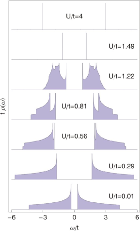
Figure 2: (Color online) Evolution of the density of states of the model for various interactions $U/t$ from strong to weak-coupling limit.

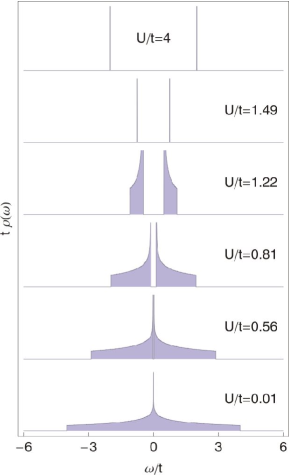
Figure 3: (Color online) Evolution of the pseudo-fermionic density of states [see, Eq. (128)] of the model for various interactions $U/t$ from strong to weak-coupling limit.

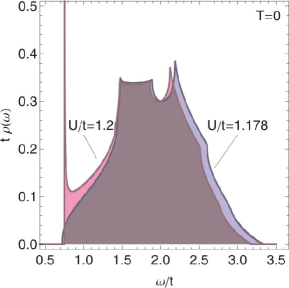
Figure 4: (Color online) Spectral weight relocation induced by change of $U/t$ interaction at zero temperature. The weight of coherence peak (equal to ${m}_{0}^{2}$) present for $U/t=1.2$ spectrum is relocated to the higher frequencies for $U/t=1.178$, so the norm (spectrum integrand over frequency) is preserved and equal to $1$.

VI Single-Particle Spectral Functions

We turn our attention now to the spectral function defined in terms of the electron Green’s function. Within our construction, it is possible to write the electron Green’s function as a product of U(1) phase, SU(2) spin (in CP¹ representation) and pseudo-fermion Green’s functions:

$$G_{z}\left(\mathbf{r}\tau,\mathbf{r}^{\prime}\tau^{\prime}\right) = -\left\langle z\left(\mathbf{r},\tau\right)\bar{z}\left(\mathbf{r}^{\prime},\tau^{\prime}\right)\right\rangle,$$

$$G_{\zeta}^{\alpha\alpha^{\prime}}\left(\mathbf{r}\tau,\mathbf{r}^{\prime}\tau^{\prime}\right) = -\left\langle\zeta_{\alpha}\left(\mathbf{r},\tau\right)\bar{\zeta}_{\alpha^{\prime}}\left(\mathbf{r}^{\prime},\tau^{\prime}\right)\right\rangle,$$

$$G_{h}^{\alpha\alpha^{\prime}}\left(\mathbf{r}\tau,\mathbf{r}^{\prime}\tau^{\prime}\right) = -\left\langle h_{\alpha}\left(\mathbf{r},\tau\right)\bar{h}_{\alpha^{\prime}}\left(\mathbf{r}^{\prime},\tau^{\prime}\right)\right\rangle,$$ (104)

while the full Green’s function of the system is the product:

$$G_{\alpha\alpha}\left(\mathbf{r}\mathbf{r}^{\prime}\tau\right) = -\sum_{\beta\gamma}\left\langle z_{\mathbf{r}}\bar{z}_{\mathbf{r}^{\prime}}\right\rangle\left\langle R_{\alpha\beta}\left(\mathbf{r}\tau\right)R_{\gamma\alpha}^{\dagger}\left(\mathbf{r}^{\prime}\tau\right)\right\rangle$$ (105)

$$\times \left\langle h_{\beta}\left(\mathbf{r}\tau\right)h_{\gamma}\left(\mathbf{r}^{\prime}\tau\right)\right\rangle.$$

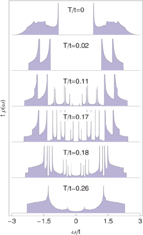
Figure 5: (Color online) Evolution of density of states as a function of the temperature (as indicated on the plot) for of $U/t=1.25$.

The problem of calculating the spectral line shapes now becomes one of calculating the convolution of the Green’s functions in Eq.(104). Since, in the antiferromagnetic phase we allow for ordering in the spin sector, the averages over spin variables can be non-zero since CP¹ Bose condensation signals the appearance of AF long-range order

$$\left\langle\bar{\zeta}_{\alpha}\left(\mathbf{k},\omega_{n}\right)\right\rangle = \left\langle\zeta_{\alpha}\left(\mathbf{k},\omega_{n}\right)\right\rangle$$ (106)

$$= \sqrt{\frac{\beta N}{2}}{m_{0}}\delta_{0,\omega_{n}}\delta_{\uparrow,\alpha}\left(\delta_{\mathbf{k},0}+\delta_{\mathbf{k},\bm{\pi}}\right),$$

where the order parameter ${m_{0}}$ measures the fraction of the condensed CP¹ bosons. Consequently, the spin Green’s function can be split into two contributions according to

$$G_{\zeta\mathbf{k}}^{\alpha\alpha}\left(\omega_{n}\right)=-\left\langle\zeta_{\alpha}\left(\mathbf{k}\omega_{n}\right)\bar{\zeta}_{\alpha}\left(\mathbf{k}\omega_{n}\right)\right\rangle$$

$$=-\left[\left\langle\zeta_{\alpha}\left(\mathbf{0}0\right)\bar{\zeta}_{\alpha}\left(\mathbf{0}0\right)\right\rangle+\left\langle\zeta_{\alpha}\left(\bm{\pi}0\right)\bar{\zeta}_{\alpha}\left(\bm{\pi}0\right)\right\rangle\right]\delta_{\omega_{n}0}\delta_{\alpha\uparrow}$$

$$-\left[1-\left(\delta_{\mathbf{k}0}+\delta_{\mathbf{k}\bm{\pi}}\right)\delta_{\omega_{n}0}\delta_{\alpha\uparrow}\right]\left\langle\zeta_{\alpha}\left(\mathbf{k}\omega_{n}\right)\bar{\zeta}_{\alpha}\left(\mathbf{k}\omega_{n}\right)\right\rangle.$$ (107)

Because, in this case the average is periodic with respect to $\mathbf{k}$:

$$\left\langle\zeta_{\alpha}\left(\mathbf{k}\omega_{n}\right)\bar{\zeta}_{\alpha}\left(\mathbf{k}\omega_{n}\right)\right\rangle=\left\langle\zeta_{\alpha}\left(\mathbf{k+\bm{\pi}}\omega_{n}\right)\bar{\zeta}_{\alpha}\left(\mathbf{k+\bm{\pi}}\omega_{n}\right)\right\rangle,$$ (108)

the spin sector Green’s function reads:

$$G_{\zeta\mathbf{k}}^{\alpha\alpha}\left(\omega_{n}\right) = -\beta N{m_{0}}^{2}\delta_{\alpha\uparrow}\delta_{\mathbf{k}0}\delta_{\omega_{n}0}$$ (109)

$$+ \left(1-2\delta_{\alpha\uparrow}\delta_{\mathbf{k}0}\delta_{\omega_{n}0}\right)G_{\zeta\mathbf{k}}^{\alpha\alpha}\left(\omega_{n}\right).$$

Substituting this result into Eq. (105) one can calculate spectral density of the system (for details, see Appendix B):

$$A_{c\mathbf{k}}^{\alpha\alpha}\left(\omega\right)=m_{0}^{2}A_{zh\mathbf{k}}^{\alpha\alpha}\left(\omega\right)$$

$$\,\,\,\,+\frac{2}{N}\sum_{\mathbf{q}\neq 0}\int_{-\infty}^{+\infty}\frac{d\omega^{\prime}}{2\pi}A_{zh\mathbf{k}-\mathbf{q}}^{\alpha\alpha}\left(\omega-\omega^{\prime}\right)A_{\zeta\mathbf{q}}^{\alpha\alpha}\left(\omega^{\prime}\right)$$

$$\,\,\,\,\times\left[n_{B}\left(-\omega+\omega^{\prime}\right)+n_{F}\left(\omega^{\prime}\right)\right]$$

$$\,\,\,\,=m_{0}^{2}A_{zh\mathbf{k}}^{\alpha\alpha}\left(\omega\right)+\sum_{\sigma}A_{zh\zeta\mathbf{k}}^{\sigma\sigma}\left(\omega\right)$$ (110)

and the density of states:

$$\rho_{c}^{\alpha\alpha}\left(\omega\right)=m_{0}^{2}\rho_{zh}^{\alpha\alpha}\left(\omega\right)+2\rho_{zh\zeta}^{\alpha\alpha}\left(\omega\right).$$ (111)

The single electron density of states contains then two terms. The first generates the the coherence peak associated with the log-range AF order, which is a product of the condensate density and the pseudo-fermion spectral function. To the extent that the peak and the background are distinguishable objects, see Fig. 2, the weight under this quasi-particle peak should be proportional to the condensate density of the CP¹ bosons. Additionally, we have calculated the density of states corresponding only to fermionic propagator $G_{h}^{\alpha\alpha}(\mathbf{k}\nu_{n})$ [see, Eq. (128)] to illustrate the correspondence between Hartree-Fock approach and our method. The outcome is presented in Fig. 3: the charge gap is a monotonic function of interaction strength $U$, which is the feature of Hartree-Fock approaches.schrieffer Upon crossing the antiferromagnetic phase boundary, one observes a remarkable feature in the spectral density plot. Figure 4 shows how the spectrum evolves upon entering the ordered magnetic state as a function of the Coulomb interaction. In a conventional Fermi liquid system, the spectrum would contain a narrow peak, which is the signature of a well-defined quasiparticle. In the AF state exactly such a peak is seen. As Fig. 4 shows, the quasiparticle peak disappears upon leaving of the ordered state. At the same time the gap is preserved, yet the narrow peak is gone. As the peak disappears the spectral weight is transferred to the incoherent excitation background. Evidently, the quasiparticle owes its existence to the of the condensation of the CP¹ bosons in the antiferromagnetic state, and not the energy gap. This exhibits a great similarity to that, which is seen in the ARPES spectra in the underdoped samples, however in this case the condensate density refers to the superconductor. The electron spectral function is very broad above the superconducting transition, but a sharp quasiparticle peak develops at the lowest binding energies, followed by a dip and a broader hump, giving rise to the so-called peak-dip-hump structure,damascelli which is very similar to our results depicted in Fig. 4, where the spectral density and density of states are sums of a coherent part consisting of convolved functions, proportional to the order parameter and incoherent – being a convolution of charge, pseudo-fermion and spin functions. It is interesting to note that the evolution of a Mott-Hubbard insulator into a correlated metal has been examined in the two-dimensional Hubbard model by using the cellular dynamical mean-field theory,kyung which incorporates short-range spatial correlations. At half filling these correlations create additional bands due to the ordered antiferromagnetic states that bear similarity to our results. As far as the comparison with earlier works based on perturbation theoryzlatic ; lamas is concerned, the main effect of correlations in the form of a transfer of the spectral weight to the high energies is reproduced. The evolution of the spectral density as a function of temperature is depicted in Fig. 5. At finite temperature there is no AF ordering according to the Mermin-Wagner theorem and consequently no coherence peak, but one observes the gap filling as the temperature increases.

VII Conclusions

In this paper we have presented a method of calculation of spectral densities for strongly correlated systems in terms of a collective phase variable, the rotating quantization axis and the fermionic degrees of freedom. In systems with strong Coulomb interactions, the phase variable dual to the local charge is an important collective field. A theory of the Hubbard model involving free fermionic degrees of freedom self consistently coupled to a quantum U(1) and SU(2) rotor model has been developed. The most interesting aspect of our approach lies however in the possibility of going beyond purely local mean-field description by incorporating the effect of spatial correlations and in particular the influence of the ordered states on the spectral properties of the system. This is very similar to the method implemented in Refs. borejsza1, ; dupuis1, , where the single-particle properties are obtained by writing the fermion field in terms of a Schwinger boson and a pseudofermion whose spin is quantized along the fluctuating Néel field. However, in the above works the charge sector was treated on the mean-field level only and the lattice was approximated by the continuous long-wave limit. In our approach, the inclusion of the antiferromagnetically ordered phase was done by resorting to the saddle-point analysis of the bosonic and fermionic effective actions, however the general architecture of the method is not resting on this assumption. The method is suitable for general value of the correlation energy $U$, which is in contrast to the TPSC methodvilk1 ; vilk2 valid in a weak-coupling limit and slave boson (fermion) approach, where the normalization of the spectral function is also violated.feng In the large-$U$ limit, the theory is controlled by the parameter $J=4t^{2}/U$, in agreement with previous approaches. Regarding the critical behavior, in the vicinity of the phase transition, our model based on the spherical approach will be equivalent to that of $n$-vector model in the limit $n\rightarrow\infty$, which is the same as in the TPSC approach. We investigated the transformation properties of Hubbard Hamiltonian leading to a symmetry adapted formulation, which explicitly exhibits the SU(2) and U(1) invariance included in the formalism. In this picture, the collective bosonic modes that represent charge and spin play an important role since the are related to the underlying symmetries of the system and the ordered states. The single-particle properties are obtained by writing the original fermion field in terms of a U(1) phase field related to the charge, CP¹ bosons that parametrize the variable quantization axis related to the rotational symmetry and a pseudo-fermion. This decomposition allows us to write down the fermion Green’s function by the product in real space of the phase, Schwinger boson propagator and the remaining fermionic propagator. Because spatial correlations are now included, we find important modifications of the electronic picture due to the formation of the ordered magnetic states. We have shown that the single electron density of states. consists of two pieces. The first generates the the peak which is a product of the condensate density of CP¹ bosons that represents the antiferromagnetic order and the and the pseudo-fermion spectral function. We found that this feature is an analog to the situation present in the normal state ARPES spectra in the underdoped samples, where the the superconducting condensate produces similar behavior.

Finally, it would be interesting to extend our calculation to the more interesting doped system, which will require additional numerical effort.

Appendix A Correlation Functions

A.1 Charge sector

The Green’s function in the charge sector reads:

$$G_{z}\left(\omega_{n}\right)=\frac{1}{\lambda_{z}+\frac{U}{8}+\frac{2}{U}\left[\omega_{n}-i\frac{U}{2}f\left(\frac{2\mu}{U}\right)\right]^{2}}.$$ (112)

Here, function $f\left(2\mu/U\right)=\mathrm{frac}\left(2\mu/U\right)-1,$ where $\mathrm{frac}\left(x\right)=x-\left[x\right]$ replaces summation over winding number in Eq. (51), which is valid for temperatures $\beta\ll U$.

A.2 Fermionic sector

In the fermionic sector, the Nambu notation of the fermionic action in Eq. (63) with vectors:

$$\bar{\Lambda}\left(\mathbf{k}\omega_{n}\right)=\left[\bar{h}_{\uparrow\mathbf{k}},\bar{h}_{\downarrow\mathbf{k}},\bar{h}_{\uparrow\mathbf{k}-\bm{\pi}},\bar{h}_{\downarrow\mathbf{k}-\bm{\pi}}\right]\left(\omega_{n}\right)$$ (113)

leads to the Green’s function matrix:

$$\mathbf{G}_{h\mathbf{k}}\left(\nu_{n}\right)=\left[\begin{array}[]{cccc}G_{h\mathbf{k}}^{\uparrow\uparrow}&0&F_{h\mathbf{k}}^{\uparrow\uparrow}&0\\ 0&G_{h\mathbf{k}}^{\downarrow\downarrow}&0&F_{h\mathbf{k}}^{\downarrow\downarrow}\\ F_{h\mathbf{k}}^{\uparrow\uparrow}&0&G_{h\mathbf{k}-\bm{\pi}}^{\uparrow\uparrow}&0\\ 0&F_{h\mathbf{k}}^{\downarrow\downarrow}&0&G_{h\mathbf{k}-\bm{\pi}}^{\downarrow\downarrow}\end{array}\right]\left(\nu_{n}\right)$$ (114)

with normal and anomalous Green’s functions

$$G_{h}^{\alpha\alpha}\left(\mathbf{k}\nu_{n}\right) = \frac{\mu+2\chi\xi_{\mathbf{k}}-i\nu_{n}}{\Delta_{c}^{2}+4\chi^{2}\xi_{\mathbf{k}}^{2}-\left(\mu-i\nu_{n}\right)^{2}},$$

$$F_{h}^{\alpha\alpha}\left(\mathbf{k}\nu_{n}\right) = \frac{\left(-1\right)^{\alpha}\Delta_{c}}{\Delta_{c}^{2}+4\chi^{2}\xi_{\mathbf{k}}^{2}-\left(\mu-i\nu_{n}\right)^{2}}.$$ (115)

A.3 Spin sector

In the spin sector, the spin action in Eq. (88) with vector

$$\bar{\Lambda}\left(\mathbf{k},\omega_{n}\right)=\left[\bar{\zeta}_{\sigma\mathbf{k}},\zeta_{\sigma-\mathbf{k}},\bar{\zeta}_{\sigma\mathbf{k}-\bm{\pi}},\zeta_{\sigma-\mathbf{k}+\bm{\pi}}\right]\left(\omega_{n}\right)$$ (116)

leads to spin Green’s function matrix:

$$\mathbf{G}_{\zeta\mathbf{k}}\left(\omega_{n}\right)=\left[\begin{array}[]{cccc}G_{\zeta\mathbf{k}},&F_{\zeta\mathbf{k}},&\tilde{G}_{\zeta\mathbf{k}},&\tilde{F}_{\zeta\mathbf{k}}\\ F_{\zeta\mathbf{k}},&G_{\zeta\mathbf{k}},&\tilde{F}_{\zeta\mathbf{k}-\bm{\pi}},&\tilde{G}_{\zeta\mathbf{k}-\bm{\pi}}\\ \tilde{G}_{\zeta\mathbf{k}},&\tilde{F}_{\zeta\mathbf{k}-\bm{\pi}},&G_{\zeta\mathbf{k}-\bm{\pi}},&F_{\zeta\mathbf{k}-\bm{\pi}}\\ \tilde{F}_{\zeta\mathbf{k}},&\tilde{G}_{\zeta\mathbf{k}-\bm{\pi}}&F_{\zeta\mathbf{k}-\bm{\pi}}&G_{\zeta\mathbf{k}-\bm{\pi}}\end{array}\right]\left(\omega_{n}\right),$$ (117)

which elements read

$$G_{\xi\mathbf{k}}\left(\omega_{n}\right) = \frac{1}{2}\left[\gamma_{-}\left(\mathbf{k},\omega_{n}\right)+\gamma_{+}\left(\mathbf{k},\omega_{n}\right)\right]$$

$$\tilde{G}_{\xi\mathbf{k}}\left(\omega_{n}\right) = \frac{1}{2}\left[\gamma_{-}\left(\mathbf{k},\omega_{n}\right)-\gamma_{+}\left(\mathbf{k},\omega_{n}\right)\right]$$

$$F_{\xi\mathbf{k}}\left(\omega_{n}\right) = -\frac{1}{2}\left[\gamma_{-}^{Q}\left(\mathbf{k},\omega_{n}\right)+\gamma_{+}^{Q}\left(\mathbf{k},\omega_{n}\right)\right]$$

$$\tilde{F}_{\xi\mathbf{k}}\left(\omega_{n}\right) = \frac{1}{2}\left[\gamma_{-}^{Q}\left(\mathbf{k},\omega_{n}\right)-\gamma_{+}^{Q}\left(\mathbf{k},\omega_{n}\right)\right],$$ (118)

where

$$\gamma_{\pm}\left(\mathbf{k},\omega_{n}\right) = \frac{\frac{\omega_{n}^{2}}{\mathcal{E}_{s}}\pm 2i\theta\omega_{n}+\lambda_{\zeta}}{\left(\frac{\omega_{n}^{2}}{\mathcal{E}_{s}}\pm 2i\theta\omega_{n}+\lambda_{\zeta}\right)^{2}-4Q^{2}\xi_{\mathbf{k}}^{2}}$$

$$\gamma_{\pm}^{Q}\left(\mathbf{k},\omega_{n}\right) = \frac{2Q\xi_{\mathbf{k}}}{\left(\frac{\omega_{n}^{2}}{\mathcal{E}_{s}}\pm 2i\theta\omega_{n}+\lambda_{\zeta}\right)^{2}-4Q^{2}\xi_{\mathbf{k}}^{2}}.$$ (119)

Appendix B Spectral densities

The Green’s function of the system is the combination of Green’s functions of charge, spin and fermionic sectors:

$$G_{c}^{\alpha\alpha^{\prime}}\left(\mathbf{r}\tau,\mathbf{r}^{\prime}\tau^{\prime}\right) = \delta_{\alpha\alpha^{\prime}}G_{z}\left(\mathbf{r}\tau,\mathbf{r}^{\prime}\tau^{\prime}\right)$$ (120)

$$\times \left[G_{\zeta}^{11}\left(\mathbf{r}\tau,\mathbf{r}^{\prime}\tau^{\prime}\right)G_{h}^{11}\left(\mathbf{r}\tau,\mathbf{r}^{\prime}\tau^{\prime}\right)\right.$$

$$+ \left.G_{\zeta}^{22}\left(\mathbf{r}\tau,\mathbf{r}^{\prime}\tau^{\prime}\right)G_{h}^{22}\left(\mathbf{r}\tau,\mathbf{r}^{\prime}\tau^{\prime}\right)\right],$$

where its Fourier transform:

$$G_{c\mathbf{k}}^{\alpha\alpha}\left(\omega_{n}\right) = \frac{1}{\beta N}\sum_{\mathbf{r}\neq\mathbf{r^{\prime}}}\int_{0}^{\beta}d\tau e^{i\mathbf{k\left(r-r^{\prime}\right)}+i\omega_{n}\left(\tau-\tau^{\prime}\right)}$$ (121)

$$\times G^{\alpha\alpha}\left(\mathbf{r}-\mathbf{r^{\prime}},\tau-\tau^{\prime}\right).$$

The spectral density is the imaginary part of the single-particle Green’s function and therefore contains full information about the temporal and spatial evolution of a single electron or a single hole in the interacting many-electron system. The spectral density is defined for fermions as follows

$$G_{X\mathbf{k}}^{\alpha\alpha}\left(\nu_{n}\right)=\int_{-\infty}^{+\infty}\frac{d\omega}{2\pi}\frac{A_{X\mathbf{k}}^{\alpha\alpha}\left(\omega\right)}{i\nu_{n}-\omega}$$ (122)

with $X=c,\,h$ for full system and fermionic sector, respectively. Similarly, for bosonic sector:

$$G_{X\mathbf{k}}\left(\omega_{n}\right)=\int_{-\infty}^{+\infty}\frac{d\omega}{2\pi}\frac{A_{X\mathbf{k}}\left(\omega\right)}{i\omega_{n}-\omega},$$ (123)

where $X=z,\zeta$ for charge and spin part. The full spectral function of the system expressed in Fourier variables is a double convolution of three elementary spectral functions of charge, spin and fermionic sectors, which written in terms of the real frequencies are

$$A_{zh\mathbf{k}}^{\alpha\alpha}\left(\omega\right) = \frac{1}{N}\sum_{\mathbf{q}}\int_{-\infty}^{+\infty}\frac{d\omega^{\prime}}{2\pi}A_{z\mathbf{q}}\left(\omega^{\prime}\right)A_{h\mathbf{k}-\mathbf{q}}^{\alpha\alpha}\left(\omega-\omega^{\prime}\right)$$

$$\times \left[n_{B}\left(-\omega^{\prime}\right)+n_{F}\left(\omega-\omega^{\prime}\right)\right]$$

$$A_{zh\zeta\mathbf{k}}^{\alpha\alpha}\left(\omega\right) = \frac{1}{N}\sum_{\mathbf{q}\neq 0}\int_{-\infty}^{+\infty}\frac{d\omega^{\prime}}{2\pi}A_{\zeta\mathbf{q}}^{\alpha\alpha}\left(\omega^{\prime}\right)A_{zh\mathbf{k}-\mathbf{q}}^{\alpha\alpha}\left(\omega-\omega^{\prime}\right)$$ (124)

$$\times \left[n_{B}\left(-\omega^{\prime}\right)+n_{F}\left(\omega-\omega^{\prime}\right)\right].$$

Introducing a density of states being a local ($\mathbf{k}$-integrated) spectral density defined as

$$\rho_{c}^{\alpha\alpha}\left(\omega\right)=-\frac{1}{2\pi N}\sum_{\mathbf{k}}A_{c\mathbf{k}}^{\alpha\alpha}\left(\omega\right),$$ (125)

one obtains convolution expressions

$$\rho_{zh}^{\alpha\alpha}\left(\omega\right) = \int_{-\infty}^{+\infty}d\omega^{\prime}\rho_{z}\left(\omega^{\prime}\right)\rho_{h}^{\alpha\alpha}\left(\omega-\omega^{\prime}\right)$$

$$\times \left[n_{B}\left(-\omega^{\prime}\right)+n_{F}\left(\omega-\omega^{\prime}\right)\right]$$

$$\rho_{zh\zeta}^{\alpha\alpha}\left(\omega\right) = \int_{-\infty}^{+\infty}d\omega^{\prime}\rho_{\zeta}^{\alpha\alpha}\left(\omega^{\prime}\right)\rho_{zh}^{\alpha\alpha}\left(\omega-\omega^{\prime}\right)$$ (126)

$$\times \left[n_{B}\left(-\omega^{\prime}\right)+n_{F}\left(\omega-\omega^{\prime}\right)\right].$$

The density of states in the charge sector reads:

$$\rho_{z}\left(\omega\right)=\frac{\delta\left(\omega-E_{c}^{-}\right)-\delta\left(\omega-E_{c}^{+}\right)}{2\sqrt{f^{2}\left(\frac{2\mu}{U}\right)+\frac{2\delta\lambda_{z}}{U}}},$$ (127)

while in the fermionic sector

$$\rho_{h}^{\alpha\alpha}\left(\omega\right) = \frac{U^{2}\left|\omega-\bar{\mu}\right|}{4t^{4}v^{2}\left(B_{+}-B_{-}\right)}\Theta\left[\left(\omega-\bar{\mu}\right)^{2}-\Delta_{c}^{2}\right]$$ (128)

$$\times \left[\rho_{2D}\left(B_{-}\right)+\rho_{2D}\left(B_{+}\right)\right]$$

with

$$B_{\pm}=\pm\frac{U\sqrt{\left(\omega-\bar{\mu}\right)^{2}-\Delta_{c}^{2}}}{2t^{2}v}.$$ (129)

In a non-dispersive case ($t=0$ or $v=0$), the fermionic density of states

$$\rho_{h}^{\alpha\alpha}\left(\omega\right)=\frac{1}{2}\delta\left(\omega-\bar{\mu}+\Delta_{c}\right)+\frac{1}{2}\delta\left(\omega-\bar{\mu}-\Delta_{c}\right).$$ (130)

In the spin sector,

$$\rho_{\zeta}\left(\omega\right)=\frac{1}{4Q}\left[\mathrm{sgn}\left(\theta-\frac{\omega}{\mathcal{E}_{s}}\right)\rho_{2D}\left(\frac{\frac{\omega^{2}}{\mathcal{E}_{s}}-\lambda_{\zeta}-2\theta\omega}{2Q}\right)\right.$$

$$\,\,\,\,\,-\left.\mathrm{sgn}\left(\theta+\frac{\omega}{\mathcal{E}_{s}}\right)\rho_{2D}\left(\frac{\frac{\omega^{2}}{\mathcal{E}_{s}}-\lambda_{\zeta}+2\theta\omega}{2Q}\right)\right],$$ (131)

where

$$\rho_{2D}\left(x\right)=\frac{\Theta\left(1-\frac{x^{2}}{4}\right)}{\pi^{2}}\mathbf{K}\left(\sqrt{1-\frac{x}{4}^{2}}\right)$$ (132)

is the density of states for the square lattice and $\mathbf{K}(x)$ stands for the complete elliptic integral of the first kind.abram

Appendix C Normalization condition

Among the general properties of the spectral function there are several sum rules. A fundamental one is

$$\int_{-\infty}^{+\infty}\frac{d\omega}{2\pi}A_{c\mathbf{k}}^{\alpha\alpha}\left(\omega\right)=1.$$ (133)

which reminds us that $A_{c\mathbf{k}}^{\alpha\alpha}\left(\omega\right)$ describes the probability of removing/adding an electron with momentum $\bf k$ and energy $\omega$ to a many-body system. Therefore, correctly calculated spectral function of the system should meet the normalization condition. We can verify this is indeed the case for the scheme presented in the present work. Since, $A_{c\mathbf{k}}^{\alpha\sigma}\left(\omega\right)$ is given by the Eq. (110), its norm reads:

$$\int_{-\infty}^{+\infty}\frac{d\omega}{2\pi}A_{c\mathbf{k}}^{\alpha\alpha}\left(\omega\right)$$

$$=\int_{-\infty}^{+\infty}\frac{d\omega}{2\pi}\left[m_{0}^{2}A_{zh\mathbf{k}}^{\alpha\alpha}\left(\omega\right)+\sum_{\sigma}A_{zh\zeta\mathbf{k}}^{\sigma\sigma}\left(\omega\right)\right].$$ (134)

Considering the first of two terms $A_{zh\mathbf{k}}^{\alpha\alpha}\left(\omega\right)$ and using the expression for the convolved charge-fermionic spectral density from Eq. (124), one obtains:

$$\int_{-\infty}^{+\infty}\frac{d\omega}{2\pi}A_{zh\mathbf{k}}^{\alpha\alpha}\left(\omega\right)=\frac{1}{N}\sum_{\mathbf{q}\neq 0}\int_{-\infty}^{+\infty}\frac{d\omega}{2\pi}\frac{d\omega^{\prime}}{2\pi}A_{z\mathbf{q}}\left(\omega^{\prime}\right)$$

$$\,\,\,\,\times A_{h\mathbf{k}-\mathbf{q}}^{\alpha\alpha}\left(\omega-\omega^{\prime}\right)\left[n_{B}\left(-\omega^{\prime}\right)+n_{F}\left(\omega-\omega^{\prime}\right)\right].$$ (135)

Transforming the integration variable $\omega\rightarrow\omega-\omega^{\prime}$ we obtain:

$$\int_{-\infty}^{+\infty}\frac{d\omega}{2\pi}A_{zh\mathbf{k}}^{\alpha\alpha}\left(\omega\right) = \frac{1}{N}\sum_{\mathbf{q}\neq 0}\left[\int_{-\infty}^{+\infty}\frac{d\omega^{\prime}}{2\pi}A_{z\mathbf{q}}\left(\omega^{\prime}\right)n_{B}\left(-\omega^{\prime}\right)\right]\left[\int_{-\infty}^{+\infty}\frac{d\omega}{2\pi}A_{h\mathbf{k}-\mathbf{q}}^{\alpha\alpha}\left(\omega\right)\right]$$ (136)

$$+ \frac{1}{N}\sum_{\mathbf{q}\neq 0}\left[\int_{-\infty}^{+\infty}\frac{d\omega^{\prime}}{2\pi}A_{z\mathbf{q}}\left(\omega^{\prime}\right)\right]\left[\int_{-\infty}^{+\infty}\frac{d\omega}{2\pi}A_{h\mathbf{k}-\mathbf{q}}^{\alpha\alpha}\left(\omega\right)n_{F}\left(\omega\right)\right].$$

Since, the charge spectral function is antisymmetric $A_{z\mathbf{q}}\left(\omega\right)=-A_{z\mathbf{q}}\left(-\omega\right)$, its integral over frequencies vanishes:

$$\int_{-\infty}^{+\infty}\frac{d\omega}{2\pi}A_{z\mathbf{q}}\left(\omega\right)=0.$$ (137)

On the other hand, the integrand of fermionic spectral density is normalized

$$\int_{-\infty}^{+\infty}\frac{d\omega}{2\pi}A_{h\mathbf{k}-\mathbf{q}}^{\alpha\alpha}\left(\omega\right)=1.$$ (138)

The remaining factor:

$$\frac{1}{N}\sum_{\mathbf{q}^{\prime}\neq 0}\int_{-\infty}^{+\infty}\frac{d\omega^{\prime}}{2\pi}A_{z\mathbf{q}^{\prime}}\left(\omega^{\prime}\right)n_{B}\left(-\omega^{\prime}\right)=1$$ (139)

is simply a charge sector constraint, which can be checked by substituting Eq. (123) to Eq. (91) and using a summation rule:

$$\frac{1}{\beta}\sum_{n}\frac{e^{i0^{-}}}{i\omega_{n}-\omega}=\frac{1}{e^{-\beta\omega}-1}=n_{B}\left(-\omega\right).$$ (140)

Finally, the first term in the Eq. (134) reads:

$$\int_{-\infty}^{+\infty}\frac{d\omega}{2\pi}A_{zh\mathbf{k}}^{\alpha\alpha}\left(\omega\right)=1.$$ (141)

Similarly, one have to treat the second term in the Eq. (134)

$$\int_{-\infty}^{+\infty}\frac{d\omega}{2\pi}A_{zh\zeta\mathbf{k}}^{\sigma\sigma}\left(\omega\right)=\frac{1}{N}\sum_{\mathbf{q}\neq 0}\int_{-\infty}^{+\infty}\frac{d\omega}{2\pi}\frac{d\omega^{\prime}}{2\pi}A_{\zeta\mathbf{q}}^{\alpha\alpha}\left(\omega^{\prime}\right)$$

$$\,\,\,\,\times A_{zh\mathbf{k}-\mathbf{q}}^{\alpha\alpha}\left(\omega-\omega^{\prime}\right)\left[n_{B}\left(-\omega^{\prime}\right)+n_{F}\left(\omega-\omega^{\prime}\right)\right].$$ (142)

Once again $A_{\zeta\mathbf{q}}^{\alpha\alpha}\left(\omega\right)=-A_{\zeta\mathbf{q}}^{\alpha\alpha}\left(-\omega\right)$, which leads to the vanishing of the integral

$$\int_{-\infty}^{+\infty}\frac{d\omega}{2\pi}A_{\zeta\mathbf{q}}\left(\omega\right)=0.$$ (143)

The remaining part is the spin sector constraint

$$\frac{1}{N}\sum_{\sigma}\sum_{\mathbf{q}^{\prime}\neq 0}\int_{-\infty}^{+\infty}\frac{d\omega^{\prime}}{2\pi}A_{\zeta\mathbf{q}^{\prime}}^{\sigma\sigma}\left(\omega^{\prime}\right)n_{B}\left(-\omega^{\prime}\right)=1-m_{0}^{2}.$$ (144)

It means that the second term in the Eq. (134) is equal to

$$\sum_{\sigma}\int_{-\infty}^{+\infty}\frac{d\omega}{2\pi}A_{zh\zeta\mathbf{k}}^{\sigma\sigma}\left(\omega\right)=1-m_{0}^{2}.$$ (145)

Substituting the results to the Eq. (134) one can see that the normalization condition from the Eq. (133) is always fulfilled. The norm of the full spectral density directly depends on the constraints in the charge and spin bosonic sectors. Therefore, careful solution of the self-consistent equations in Sec. V is of primary importance to obtain physically reasonable results.

References

• (1) A. Damascelli, Z. Hussain, and Z.-X. Shen, Rev. Mod. Phys. 75, 473 (2003).
• (2) J. Hubbard, Proc. Roy. Soc. A 276, 238 (1963); N. F. Mott, Metal-insulator transitions (Taylor and Francis, London, 1990).
• (3) M.B. J. Meinders, H. Eskes, and G.A. Sawatzky, Phys. Rev. B 48, 3916 (1993).
• (4) V. Zlatić, K. D. Schotte, and G. Schliecker, Phys. Rev. B 52, 3639 (1995).
• (5) C. A. Lamas, arXiv:0708.4344v2.
• (6) N. Bulut, D. J. Scalapino, and S. R. White, Phys. Rev. Lett. 72 705 (1994);
• (7) A. Moreo, S. Haas, A. W. Sandvik, and E. Dagotto, Phys. Rev. B 51 12045 (1995);
• (8) R. Preuss, W. Hanke, and W. von der Linden, Phys. Rev. Lett. 75 1344 (1995);
• (9) N. S. Vidhyadhiraja, A. Macridin, C. Sen, M. Jarrell, and M. Ma, arXiv:0809.1477v1.
• (10) O. Juillet, New J. Phys. 9 163 (2007).
• (11) N. Bulut, Advances in Physics 51, 1587 (2002).
• (12) A. Georges, G. Kotliar, W. Krauth, and M. Rozenberg, Rev. Mod. Phys. 68, 13 (1996).
• (13) Th. Maier, M. Jarrel, Th. Pruschke, and M.H. Hettler, Rev. Mod. Phys. 77, 1027 (2005).
• (14) Y.M. Vilk, and A.-M.S. Tremblay, J. Phys. I France 7, 1309 (1997);
• (15) Y.M. Vilk, L. Chen, and A.-M.S. Tremblay, Phys. Rev. B 49 13267 (1994).
• (16) A.V. Chubukov, A.M. Finkelstein, R. Haslinger, and D.K. Morr, Phys. Rev. Lett.90, 077002 (2003); A. V. Chubukov, Phys. Rev. B71, 245123 (2005).
• (17) K. Borejsza, and N. Dupuis, Phys. Rev. B 69 085119 (2004).
• (18) N. Dupuis, Phys. Rev. B bf 65 245118 (2002).
• (19) T.A. Zaleski and T.K. Kopeć Phys. Rev. B 77, 125120 (2008).
• (20) M.V. Berry, Proc. R. Soc. London, Ser. A 392, 451 (1984).
• (21) H.J. Schulz, Phys. Rev. Lett. 65, 2462 (1990).
• (22) J. Hubbard Phys. Rev. Lett. 3, 77 (1959); R.L. Stratonovich, Sov. Phys. Doklady 2 416 (1958).
• (23) V.N. Popov, Functional integrals and collective excitations (Cambridge Univesity Press, 1987).
• (24) L.S. Schulman, Techniques and Applications of Path Integration (Wiley, New York, 1981).
• (25) T.K. Kopeć, Phys. Rev. B 72, 132503 (2005).
• (26) H. Schoeller and G. Schön, Phys. Rev. B 50, 18436 (1994).
• (27) E. Fradkin, Field Theories of Condensed Matter Systems (Addison Wesley, Reading, 1991).
• (28) T.K. Kopeć, Phys. Rev. B 73, 104505 (2006).
• (29) M.C. Gutzwiller, Phys. Rev. Lett. 10, 159 (1963). M.C. Gutzwiller, Phys. Rev. 137, A1726 (1965).
• (30) A.V. Chubukov, D.M. Frenkel, Phys. Rev. B 46, 11884 (1992).
• (31) A. Auerbach, Interacting Electrons and Quantum Magnetism (Springer–Verlag, New York, 1994).
• (32) J.C. Slater, Phys. Rev. 82, 538 (1951).
• (33) N.D. Mermin and H. Wagner, Phys. Rev. Lett. 17, 1133 (1966).
• (34) J.R. Schrieffer, X.G. Wen, and S.C. Zhang, Phys. Rev. B 39, 11663 (1989).
• (35) A. Damascelli, Z. Hussain, and Z.-X. Shen, Rev. Mod. Phys. 75 473 (2003).
• (36) B. Kyung, S. S. Kancharla, D. Sénéchal, A.-M. S. Tremblay, M. Civelli, and G. Kotliar, Phys. Rev. B 73 165114 (2006).
• (37) S. Feng, J.B. Wu, Z.B. Su, and L. Yu, Phys. Rev. B 47 15192 (1993).
• (38) M. Abramovitz and I. Stegun, Handbook of Mathematical Functions (Dover, New York, 1970).