Quantum Mechanics and Nonlocality:
In Search of Instructive Description

Abstract

A problem with an instructive description of measurement process for sufficiently separated entangled quantum systems is well known. More precise and crafty experiments together with new technological challenges raise questions about sufficiency of formal use of “black-box” Copenhagen paradigm without subtleties of transition between quantum and classical worlds. In this work are discussed applications both standard interpretation of quantum mechanics and “unconventional” models, like relative state formulation, multiple clocks formalism, and extended probabilities.

1 Introduction

There are certain problems with description of nonlocality in quantum mechanics. A “black-box” scheme of a standard experiment is represented on Fig. 1: initially interacting quantum systems are separated on some distance and two independent measurements are performed after that.

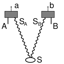
Figure 1: Scheme of measurement

In a conclusion to a description of an experimental test of “realism” conception in quantum mechanics, performed not so long time ago [1] was mentioned, that these “results lend strong support to the view that any future extension of quantum theory that is in agreement with experiments must abandon certain features of realistic descriptions.” Rather broad notion of the realistic description may be found in very beginning of the same paper [1]: “Physical realism suggests that the results of observations are a consequence of properties carried by physical systems.”

It looks like suggestion for any future extension of quantum theory to evade ideas about results of observation as a consequence of properties carried by physical systems. The claim about limitations on “realism” considered in [1] is more strong, than in most other works, because it is “experimentally excluded” both local models and “a class of important non-local hidden-variable theories.” It is also mentioned, that non-local models outside of this class are “highly counterintuitive.”

On the other hand, yet another experiment suggested in [2, 3, 4] may be considered as an illustration, that paradox of quantum nonlocality may be irrelevant with discussions about reality of wave functions or density matrixes. The Conway-Kochen Free State (Free Will) theorem [2] is formulated about results of observations and so illustration of a problem is transferred to classical level.

Formally, it even does not matter for SPIN and TWIN axioms [2], if the measurements are a consequence of quantum or classical properties carried by physical systems or not. Only FIN axiom about finite speed of information transfer [2] or MIN axiom about locality [4] include some suggestions about properties of physical processes.

Problem with locality demonstrated by Conway-Kochen theorem is not produced by realism or any other property of physical model. An advantage of such result declared in [2] “is that it applies directly to the real world rather than just to theories. It is this that prevents the existence of local mechanisms for reduction.”

In order to avoid discussions about free will [2, 3, 4, 5, 6] it could be suggested few explanations:

1. Nonlocality.

2. Some effects (e.g., relativistic, stochastic, etc.) obstructing possibility to use abridged version of quantum theory expressed by SPIN, TWIN postulates [2].

3. Inapplicability of suggestion about definite outcomes (e.g., theories without reduction like Everett formulation).

So, from the one hand, there are ideas about necessity to abandon realism to have an agreement with experiment [1], but from the other hand there is no any guarantee about resolution of problems with consistent description of more complicated tests [2]. It could be even said informally, that if classical notion of realism “is not enough” to establish interdependences displayed by quantum systems, then the idea to “abandon certain features of realistic descriptions” may be a step in a wrong direction.

The purpose of presented excursus was not a criticism of some particular ideas, but demonstration of rather objective difficulties in modern interpretations of experiments with a few quantum systems. Nowadays quantum physics displays enormous progress in predicting and explaining of properties of elementary quantum particles, but already description of two simplest quantum systems may raise conceptual problems illustrated above.

Contents:

In Sec. 2 is reminded simple nonlocal model of measurement for arbitrary quantum system with finite-dimensional space of states. Nowadays such kind of models ensures possibility to use classical computer for modeling of not very large quantum systems in quantum information science. Problem with nonlocality may be formally avoided in formulations without collapse and it is discussed in Sec. 3. Particular example of entangled spin-1 particles used in Conway-Kochen theorem is developed for the “no-collapse” formulation in App. B.

Sec. 4 is devoted to introduction of two-time (or, rather, two-clocks) formalism earlier suggested by Bell for description of EPR paradox and GRW models. Von Neumann measurement scheme is applied further in Sec. 5 and problem of definite outcomes is revisited in Sec. 6. This problem is especially illustrative for Conway-Kochen scheme with two entangled spin-1 particles discussed in Sec. 7 and App. A.

Feynman ideas about negative probabilities are affected in Sec. 8 and App. C with concrete example of decomposition with positive and negative terms for entangled state of two spin-1 particles. Finally, in Sec. 9 is touched upon a relation of nonlocality and inseparability in quantum mechanics.

2 Simple Nonlocal Model

A simple nonlocal hidden variable model for discussed experiments is known and may be even considered as direct consequence of quantum mechanical definitions.

Let us discuss briefly such a model for experiments with two possible outcomes of each measurement like [1]. If there are known equations for probabilities ($P_{1}\equiv P_{++}$, $P_{2}\equiv P_{+-}$, $P_{3}\equiv P_{-+}$, $P_{4}\equiv P_{--}$) for four possible combinations of events like $\sf a=\pm 1$ and $\sf b=\pm 1$ we may use “roulette” Fig. 2 with four sectors proportional to given probabilities and angle of rotation of pointer is corresponding to a hidden variable $0\leq\phi<2\pi$. Pair of outcomes is defined by pairs of indexes $(+1,+1)$, $(+1,-1)$, $(-1,+1)$, $(-1,-1)$ assigned with each sector of the roulette.

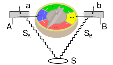
Figure 2: Nonlocal hidden variables model

It is usual example of a model for generation of given probability distribution for known probabilities and so it may be considered as rather “mechanical” consequence of Born rules with squares of modules of quantum amplitudes. But this “minimal” model is really counterintuitive for separated systems because for application of such “nonlocal roulette” it is necessary to know parameters of measurements for both parties A and B.

In general case there are set of probabilities $P_{\sf ab}$ defined for entangled state $\Psi$ and projectors $\hat{\mathtt{P}}_{\sf a}$ and $\hat{\mathtt{P}}_{\sf b}$ with equation like

$$P_{\sf ab}=\langle\Psi|\hat{\mathtt{P}}_{\sf a}\otimes\hat{\mathtt{P}}_{\sf b}|\Psi\rangle.$$ (2.1)

For a product state $|\Phi\rangle=|\psi\rangle|\phi\rangle$ it is possible to write

$$P_{\sf ab}=\langle\Phi|\hat{\mathtt{P}}_{\sf a}\otimes\hat{\mathtt{P}}_{\sf b}|\Phi\rangle=\langle\psi|\hat{\mathtt{P}}_{\sf a}|\psi\rangle\langle\phi|\hat{\mathtt{P}}_{\sf b}|\phi\rangle=P_{\sf a}P_{\sf b},\quad P_{\sf a}=\langle\psi|\hat{\mathtt{P}}_{\sf a}|\psi\rangle,~{}P_{\sf b}=\langle\phi|\hat{\mathtt{P}}_{\sf b}|\phi\rangle.$$ (2.2)

In classical probability theory Eq. (2.2) $P_{\sf ab}=P_{\sf a}P_{\sf b}$ corresponds to independent events and may be modeled with two local roulettes.

It is also possible to reproduce correlated events, if to use analogue of classical equation for conditional probabilities [7]

$$\textstyle P(a,b)=P(a)P(b|a)=P(b)P(a|b),$$ (2.3)

and instead of model with two correlated events $P(a,b)\equiv P_{\sf ab}$ Eq. (2.1) (Fig. 3a), one event is considered as local one with probability $P_{\sf a}$ and the second one is dependent event with conditional probability $P_{\sf b|a}=P_{\sf ab}/P_{\sf a}$ (Fig. 3c). It is also possible to use an opposite order of events with probabilities $P_{\sf b}$ and $P_{\sf a|b}=P_{\sf ab}/P_{\sf b}$ (Fig. 3b). Equations for $P_{\sf a}$ and $P_{\sf b}$ for given entangled state $|\Psi\rangle$ may be written directly

$$P_{\sf a}=\langle\Psi|\hat{\mathtt{P}}_{\sf a}\otimes\hat{\mathtt{1\!\!I}}|\Psi\rangle,\quad P_{\sf b}=\langle\Psi|\hat{\mathtt{1\!\!I}}\otimes\hat{\mathtt{P}}_{\sf b}|\Psi\rangle$$ (2.4)

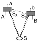
a) b) c)

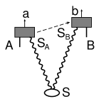
Figure 3: Schemes of possible dependencies

Such nonsymmetrical models are even more known due to direct analogue with Einstein-Podolsky-Rosen consideration [8] evolved further in many modifications [9] and intensively tested and analyzed till nowadays [10]. The arrows on Fig. 3b,c correspond to Einstein’s “spooky action at a distance” or “SF mechanism” [11].

3 Everett’s Formulation

A known method to resolve the problem with nonlocality is Everett’s formulation of quantum mechanics [12, 13, 14, 15] and due to difficulties with standard interpretation, it devotes an accurate consideration. An essential idea Fig. 4 is a claim, what correlations are uncovered by some local operation of comparison C Fig. 4a.

a)   b)

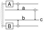
Figure 4: Alternative scheme of measurements

A concrete calculations for two spin-half systems may be found in [13, 14, 15] with a scheme of quantum network like Fig. 4b [13]. Analogous model for spin-1 systems used in Conway-Kochen (thought) experiment is discussed below in App. B

In a quantum network model each system denoted as a line (“wire”) and an unitary operator as a “gate” on one () or two () systems. Such a scheme Fig. 4b illustrates an additional carriers a and b used for resolution of nonlocality problem.

It is not even necessary to completely accept Everett’s formulation. Minimal implication of such a model may be suggestion, that it is enough to have entangled outcomes of measurements to explain quantum correlations.

It may be also raised a question about necessity of such entanglement. Really, all the nonclassical correlations, inequalities and paradoxes may be derived from quantum superposition principles. Is it possible to explain the correlations between nonlocal outcomes without entanglement, i.e., special kind of superposition?

It is possible to consider a question about treatment of some quantum correlations as an experimental test of Everett’s interpretation. Yet, such a confirmation of macroscopic superposition of different states of measurement devices is rather indirect in comparison with other modern experiments providing “powerful examples for the validity of unitary Schrödinger dynamics and the superposition principle on increasingly large length scales” [16].

Such indirect evidence could be justified only after proof on impossibility of other explanations of observed effects. More direct proof should include description, analysis and testable consequences of explicit models for reduction process.

It may appears, that relativity principle prevent any reasonable “internal” description of reduction for space-like separated measurements of two observers and it is necessary to act in spirit of Copenhagen interpretation and only talk about (classical) final results or probabilities. But even lack of possibility to introduce some order for such measurements may be overcome in description with local clocks.

4 Formalism with Local Clocks

The local clocks, i.e., application of two-time formalism to discussion about quantum nonlocality is not a new idea, e.g., it is represented in two last chapters of collection of Bell’s papers [17].

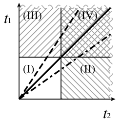
a)   b)

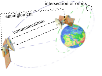
Figure 5: Model with local clocks

A classical probability (density) for two particles to have positions $x_{1}$ and $x_{2}$ is represented by a function $\varrho(x_{1},x_{2})$. A dynamical process is usually described via some function $\varrho(x_{1},x_{2},t)$. If there is some reason to use separate clocks for each particle, it is possible to introduce a function $\varrho(x_{1},t_{1},x_{2},t_{2})$.

Similar function $\varrho(x_{1},t_{1},x_{2},t_{2})=\bigl{|}\psi(x_{1},t_{1},x_{2},t_{2})\bigr{|}^{2}$ may be used in quantum mechanics for description of nonlocality in EPR correlations [17, §21] or GRW models [17, §22]. Here the same approach is used for description of measurement for two parties, if order of event is not defined.

Let $\hat{\rho}(x_{1},t_{1},x_{2},t_{2})$ is a density matrix for such a system. It is suggested, that measurement is performed by each party on time $\tau$ on local clock. So there are four zones on “two-time plane” Fig. 5a: (I) $t_{1}<\tau,\ t_{2}<\tau$, (II) $t_{1}<\tau,\ t_{2}\geq\tau$, (III) $t_{1}\geq\tau,\ t_{2}<\tau$, (IV) $t_{1}\geq\tau,\ t_{2}\geq\tau$.

Quite realistic example of such a scheme is entangled state used in experiments with satellites Fig. 5b. Difference between clocks due to relativistic effects in principle may be essential in modern experiments. Three lines (solid, dashed, dash-and-dot) on Fig. 5a represent different method of synchronization of $t_{1}$ and $t_{2}$ with some global clock $t$.

Equipment on both satellites may be programmed to performs measurement at the same time $\tau$ on local clocks, but order is not an absolute property due to relativity principle. Quantum cryptography with entangled states and free space communications [18] may make such schemes quite actual. Even if pair of entangled qubits used in such communications is not relevant with particular scheme suggested in [2], systems of quantum cryptography with qutrits [19, 20] are already valid area for such a discussion.

Let us denote measurement procedures as ${\tt M}_{\sf A}$ and ${\tt M}_{\sf B}$ for first and second party respectively. If initially there is some density matrix $\hat{\rho}$ and it is changed only due to measurements, then for each zone it may be written $\hat{\rho}_{I}=\hat{\rho}$, $\hat{\rho}_{II}={\tt M}_{\sf B}\hat{\rho}$, $\hat{\rho}_{III}={\tt M}_{\sf A}\hat{\rho}$, and for independent measurements $\hat{\rho}_{IV}={\tt M}_{\sf A}{\tt M}_{\sf B}\hat{\rho}={\tt M}_{\sf B}{\tt M}_{\sf A}\hat{\rho}$.

5 Von Neumann Measurements

The measurements above are presented in rather abstract way. It is possible first to consider von Neumann measurement [21] defined for single system and a measurement basis $\varphi_{k}$ as a linear map

$$\hat{\rho}\mapsto\sum_{k}\langle\varphi_{k}|\hat{\rho}|\varphi_{k}\rangle\hat{\mathtt{P}}_{[\varphi_{k}]},\quad\hat{\mathtt{P}}_{[\varphi_{k}]}\equiv|\varphi_{k}\rangle\langle\varphi_{k}|.$$ (5.1)

For more general case of incomplete von Neumann measurement [22] it may be rewritten as

$$\hat{\rho}\mapsto\breve{\mathtt{\Pi}}(\hat{\rho})=\sum_{m}\breve{\mathtt{\Pi}}_{m}(\hat{\rho}),\quad\breve{\mathtt{\Pi}}_{m}(\hat{\rho})=\hat{\mathtt{P}}_{m}\hat{\rho}\,\hat{\mathtt{P}}_{m},$$ (5.2)

where $\hat{\mathtt{P}}_{m}$ is not necessary one-dimensional projector. Now it is possible to define measurements for two-parties system

$${\tt M}_{\sf A}=\breve{\mathtt{\Pi}}_{\sf A}\otimes\breve{\mathtt{1\!\!I}},\quad{\tt M}_{\sf B}=\breve{\mathtt{1\!\!I}}\otimes\breve{\mathtt{\Pi}}_{\sf B},$$ (5.3)

where $\breve{\mathtt{1\!\!I}}=\hat{\mathtt{1\!\!I}}$ is identity (“unit superoperator”), $\breve{\mathtt{\Pi}}_{\sf A}$ and $\breve{\mathtt{\Pi}}_{\sf B}$ are defined by Eq. (5.2) using set of projectors for measurements of ${\sf A}$ and ${\sf B}$.

Let us consider an example with two possible decompositions of the same entangled state

$$|\Psi\rangle=\sum_{k}\alpha_{k}|a_{k}\rangle|u_{k}\rangle=\sum_{j}\beta_{j}|v_{j}\rangle|b_{j}\rangle,$$ (5.4)

there $|a_{k}\rangle$ and $|b_{j}\rangle$ are measurement bases chosen by ${\sf A}$ and ${\sf B}$ respectively. It is now possible to find values of density matrixes in all four zones:

$$\hat{\rho}_{I}=\hat{\rho}_{[\Psi]}=|\Psi\rangle\langle\Psi|,$$ (_I)

$$\textstyle\hat{\rho}_{II}=\sum_{j}|\alpha_{j}|^{2}\,|v_{j}\rangle\langle v_{j}|\otimes|b_{j}\rangle\langle b_{j}|,$$ (_II)

$$\textstyle\hat{\rho}_{III}=\sum_{k}|\beta_{k}|^{2}\,|a_{k}\rangle\langle a_{k}|\otimes|u_{k}\rangle\langle u_{k}|,$$ (_III)

$$\textstyle\hat{\rho}_{IV}=\sum_{k,j}q_{kj}\,|a_{k}\rangle\langle a_{k}|\otimes|b_{j}\rangle\langle b_{j}|,$$ (_IV)

where $q_{kj}$ in Eq. (_IV) is some matrix. It may be expressed in two different ways

$$q_{kj}=\bigl{|}\alpha_{j}\langle a_{k}|v_{j}\rangle\bigr{|}^{2}=\bigl{|}\beta_{k}\langle u_{k}|b_{j}\rangle\bigr{|}^{2}$$ (5.6)

using Eq. (_II) and Eq. (_III) respectively.

It is possible to use particular symmetric case of Eq. (5.4)

$$|\Upsilon\rangle=\frac{1}{\sqrt{N}}\sum_{k=1}^{N}|a_{k}\rangle|a_{k}\rangle=\frac{1}{\sqrt{N}}\sum_{k=1}^{N}|b_{k}\rangle|b_{k}\rangle,$$ (5.7)

appropriate for discussion on Conway-Kochen theorems [2] (see Eq. (B.3) and Eq. (B.5) in App. B). In such a case Eq. (5.5) become simpler

$$\hat{\rho}_{I}=\hat{\rho}_{[\Upsilon]}=|\Upsilon\rangle\langle\Upsilon|,$$ (_I)

$$\textstyle\hat{\rho}_{II}=N^{-1}\sum_{j=1}^{N}|b_{j}\rangle\langle b_{j}|\otimes|b_{j}\rangle\langle b_{j}|,$$ (_II)

$$\textstyle\hat{\rho}_{III}=N^{-1}\sum_{k=1}^{N}|a_{k}\rangle\langle a_{k}|\otimes|a_{k}\rangle\langle a_{k}|,$$ (_III)

$$\textstyle\hat{\rho}_{IV}=N^{-1}\sum_{k,j=1}^{N}\bigl{|}\langle a_{k}|b_{j}\rangle\bigr{|}^{2}|a_{k}\rangle\langle a_{k}|\otimes|b_{j}\rangle\langle b_{j}|,$$ (_IV)

Scheme of measurement Fig. 5a may be represented

$$\begin{array}[]{ccc|cc}{}^{(III)}&(\!(a,a)\!)&\longrightarrow&{}^{(IV)}&(\!(a,b)\!)\\ \hline\cr&\uparrow&\nearrow&&\uparrow\\ {}_{(I)}&\hat{\rho}_{[\Upsilon]}&\longrightarrow&{}_{(II)}&(\!(b,b)\!)\\ \end{array}$$ (5.9)

where $(\!(\cdot,\cdot)\!)$ is brief notation for sums in Eq. (5.8) and also may be considered in more general sense as an abstract representation of result of measurement(s).

6 Definite Outcomes

Introduction of von Neumann measurement only partially illustrates problem of reduction. It is used description of ensembles and transition between quantum mechanical description and classical statistical properties are given by known equations, like Born rule. Nonlocality of such equations is often demonstrated only indirectly and related with additional assumptions about class of reasonable local models [23, 24, 25].

Formally, description with ensembles still contains some analogue of multiple world formalism, because it is yet some equation with superposition of different states. The problem becomes more difficult, if to try to find a method for generation of certain outcome for each measurement. It is called sometimes the problem of definite outcomes [26].

In quantum mechanical description without reduction such a question looks incorrect, because there is no certain outcome in superposition. In description with ensembles such question may be correct, but often is weaved as something inappropriate. It is analogue of classical statistical theory with description of probabilities, but not reasons for given outcome in single test.

More abstract measure theory may represent an alternative view, then distribution of probabilities decribes all possible outcomes with different measure of “actuality.” Bell represents usual argument against such a view [17, §11] “Whereas Everett assumes that all configurations of his special variables are realized at any time, each in the appropriate branch universe, the de Broglie world has a particular configuration. I do not myself see that anything useful is achieved by the assumed existence of the other branches of which I am not aware.”

In cited paper Bell just discussed de Broglie-Bohm theories, i.e., models with possibility to assign certain outcome to each measurement. Certainly, usual scientific principle of “Occam’s razor” demands to “cut” all extra branches. On the other hand, we may be not aware about some phenomena, but have to accept that as most reasonable way to explain observed things.

The problem with suggestion about only one term in superposition may be illustrated with Conway-Kochen experiment [2]. It may be used particular case of Eq. (5.7) with three terms.

$$\Upsilon=\frac{1}{\sqrt{3}}\bigl{(}|1\rangle|1\rangle+|2\rangle|2\rangle+|3\rangle|3\rangle\bigr{)}$$ (6.1)

See App. A and App. B and Ref. [27] for more details.

First observer uses for measurement three basic states $|x\rangle$, $|y\rangle$ and $|z\rangle$ simply associated with three orthogonal axes and second observer is using $|x^{\prime}\rangle$, $|y^{\prime}\rangle$, and $|z^{\prime}\rangle$. Let’s consider particular situation with $|x^{\prime}\rangle=|y\rangle$, $|y^{\prime}\rangle=(|x\rangle+|z\rangle)/\sqrt{2}$, $|z^{\prime}\rangle=(|x\rangle-|z\rangle)/\sqrt{2}$.

Final (in “zone IV”) distribution of probabilities Eq. (_IV) may be represented by table

$$\frac{1}{3}\left(\begin{array}[]{ccc}\bigl{|}\langle x|x^{\prime}\rangle\bigr{|}^{2}&\bigl{|}\langle x|y^{\prime}\rangle\bigr{|}^{2}&\bigl{|}\langle x|z^{\prime}\rangle\bigr{|}^{2}\\ \bigl{|}\langle y|x^{\prime}\rangle\bigr{|}^{2}&\bigl{|}\langle y|y^{\prime}\rangle\bigr{|}^{2}&\bigl{|}\langle y|z^{\prime}\rangle\bigr{|}^{2}\\ \bigl{|}\langle z|x^{\prime}\rangle\bigr{|}^{2}&\bigl{|}\langle z|y^{\prime}\rangle\bigr{|}^{2}&\bigl{|}\langle z|z^{\prime}\rangle\bigr{|}^{2}\\ \end{array}\right)=\frac{1}{3}\left(\begin{array}[]{ccc}0&0.5&0.5\\ 1&0&0\\ 0&0.5&0.5\\ \end{array}\right)$$ (6.2)

In table Eq. (6.2) some combinations of outcomes have zero probabilities in zone (IV), e.g., $(\!(x,x^{\prime})\!)$. On the other hand, impossibility to have outcome $x$ for first observer is certain only for particular choice of the second one. In zone (III) outcomes $x$, $y$ and $z$ have equal weights, but may be impossible in combination with certain choice and outcome of second observer. The analogue is true for second observer, zone (II).

If to keep all terms in superposition, it could be considered as some formal redistribution, like $(1/3,1/3,1/3)\mapsto(1,0,0)$ or $(1/3,1/3,1/3)\mapsto(0,1/2,1/2)$, where combinations like $(\!(x,x^{\prime})\!)$ are excluded from final mixture at all. With definite outcome for each observer it is not clear, why the impossible pairs like $(\!(x,x^{\prime})\!)$ could not be produced, if both $x$ and $x^{\prime}$ are valid outcomes.

7 Conway-Kochen Theorems

Example below raises question about possibility to test existence of “invisible terms” indirectly. Such a question lay beyond the limits of quantum theory, there is not defined a receipt to choose and save only single term in some superposition. It may be discussed in some extensions like de Broglie-Bohm theories already mentioned above in Bell’s cite or Ghirardi-Rimini-Weber (GRW) models [28].

In [2, 3, 4] problem of nonlocal measurements was analysed also with relation to GRW theories and it was shown, that for wide class of theories (“Free State theories”) it is impossible to suggest local method to provide certain outcomes for pair of measurements of some entangled state in agreement with SPIN and TWIN axioms, considered as simple consequence of quantum theory.

It may be shown, that both SPIN and TWIN axioms formally do not respect Lorentz invariance [29], and so it is better to use limit of small speeds and formulation without appeal for relativity, like [4]. After all, only field theory may properly take into account relativistic effects [30] and so reasoning about isolated pair of particles may have some flaws. Yet another criticism may be found in [31, 32].

In fact, problem with “reconciliation” of quantum mechanics and special relativity is well known. One subject of Nobel Prize Lecture Asymptotic freedom: From paradox to paradigm [33] by Frank Wilczek in 2004 had quite illustrative title: “Paradox 2: Special Relativity and Quantum Mechanics Both Work” and declared “creative tension” of such paradoxes, leading to four Nobel Prizes (1933, 1965, 1999, 2004).

So Conway-Kochen arguments illustrating some problems with nonlocality even in nonrelativistic quantum mechanics [4] devote accurate consideration, especially because it is not suggested yet, how the field theory could avoid that.

A consequence of Conway-Kochen theorem necessary for present purpose is absence of “reasonable” local model with definite outcomes for state Eq. (6.1) with three terms. In [2, 3, 4] instead of term “reasonable” was used idea of “free state theories” describing “the evolution of a state from an initial arbitrary or “free” state according to laws that are themselves independent of space and time” [2]. In App. A is reproduced some arguments to do not limit problem in such a way and to use “any” instead of “reasonable” above.

Anyway, experiment with two entangled spin-1 particles suggested by Conway and Kochen [2, 3, 4] is very hard to explain by some analogue of de Broglie-Bohm theory and so argument of Bell et al against Everett multiple world formalism is not strong enough, because models with single branch may look much more weird than multiverse “science fiction.”

Authors of [2, 3, 4] are embarked in discussion about free will of particles and experimenters, but it is possible to suggest analogues of they theorems without any relation with possibility of free choice. It is also possible to argue, what accepting “free will” for particles in given experimental setup would produce possibility of superluminal information exchange, because it is suggested some coordinated choice between pair of outcomes like (0,0) or (1,1).

It is clear from analysis of [2, 3, 4] that even using instead of particles two intelligent human gamblers (Carl and Clara) with free will and perfect knowledge of quantum mechanics could not establish necessary correlations (if to exclude cooperation with Alice and Bob like preliminary agreement about setup of all future measurements). So term “free will” in [2, 3, 4] is rather used for some mysterious and subtle ability to make right choice without necessary information.

Here Conway-Kochen result is discussed due to very clear demonstration of contradiction between nonlocality and correlation of definite outcomes. In [2, 3, 4] a possibility of macroscopic quantum superposition between results of measurements is even not considered, but it is valid explanation of necessary correlations compatible with quantum mechanics.

A bias against Everett interpretation is so strong, that as more appropriate explanation are considered almost supernatural properties of elementary particles [2, 3, 4]. In [34] is suggested more “precise” statement of related idea: “quantum randomness can be controlled by influences from outside spacetime, and therefore by immaterial free will.”

The purpose of given paper is not an apology for multiverse. The idea of multiverse looks like some try of classical reasoning about quantum superposition in single universe. The more precise statement of problem is possibility to use macroscopic superposition of measurement outcomes as an explanation of quantum correlations observed in experiments.

Such macroscopic superposition may not be accepted without doubts. The possible loopholes often discussed in relation with local hidden variables models [35]. As an support for possibility of future achievements in next section is reproduced yet another “extravagant” local model.

It is astonishingly yet, that problem with theoretical model of reduction and definite outcomes may convert interpretation of many experiments claiming confirmation of quantum correlations with too high precision into argument against “standard” interpretation and an additional evidence for Everett’s formulation (if other alternatives may be even more strange). It may be considered as an argument to revisit results of even standard experiments with more attention [36].

8 Extended Probabilities

Quantum state of composite system is called separble [22] if density matrix may be represented as sum

$$\rho=\sum_{k}\lambda_{k}\rho_{k}^{\sf A}\otimes\rho_{k}^{\sf B},\quad\lambda_{k}>0.$$ (8.1)

For such a state nonlocal measurement discussed above may be modeled by local model, if to suggest that source emits different pairs of states $\rho_{k}^{\sf A}\otimes\rho_{k}^{\sf B}$ with probabilities $\lambda_{k}$.

On the other hand, if to exclude requirement about positivity of $\lambda_{k}$ in Eq. (8.1) any state may be represented as [38, 39]

$$\rho=\sum_{k=1}^{n^{+}}\lambda^{+}_{k}\hat{\rho}_{k}^{\sf A}\otimes\hat{\rho}_{k}^{\sf B}-\sum_{k=n^{+}+1}^{n^{+}+n^{-}}|\lambda^{-}_{k}|\,\hat{\rho}_{k}^{\sf A}\otimes\hat{\rho}_{k}^{\sf B}=\kappa\hat{\rho}^{+}-(\kappa-1)\hat{\rho}^{-},\quad\lambda^{+}_{k}>0,\quad\kappa=\sum_{k=1}^{n^{+}}\lambda^{+}_{k}$$ (8.2)

with $\hat{\rho}^{+}$ and $\hat{\rho}^{-}$ are two separable states. In App. C is shown such representation of state Eq. (6.1) for $N=3$ with $n^{+}=18$, $n^{-}=15$, and $\kappa=7$.

Association of entangled states with negative probability is not a new thing. Talk of Feynman about such negativity for Bell state [40] on PhysComp’81 may be included into origins of modern quantum information science and quantum cryptography. It was also discussed by Bell in a paper about two-time Wigner distribution and EPR already mentioned above [17, §21].

Figure 6: Venn diagram for ${\sf A}$, ${\sf B}$, ${\sf A}\cup{\sf B}$, ${\sf A}\cap{\sf B}$

In later paper [41] Feynman mentioned more examples in classical and quantum mechanics to conclude “…conditional probabilities and probabilities of imagined intermediary states may be negative in a calculation of probabilities of physical events and states.” Mathematical justification for such formalism is theory of signed measures (charges) [42]. Another trivial example is usual classical equation for calculation of probability for union of two overlapped classes of events $P({\sf A}\cup{\sf B})=P({\sf A})+P({\sf B})-P({\sf A}\cap{\sf B})$ [7] with negative sign before probability of events in class ${\sf A}\cap{\sf B}$, see Fig. 6.

Table Eq. (C.3) in App. C shows signed decomposition Eq. (8.2) for a state $|\Upsilon\rangle$ Eq. (6.1) used in examples above and related with Conway-Kochen theorems. For given state and choice of basis in space of density matrixes there are 18 positive and 15 negative terms. Formally, it is possible to use a local theory for calculation of some averages for physical values in agreement with quantum mechanics. Really, it is possible to represent

$$\hat{\rho}_{[\Upsilon]}\equiv|\Upsilon\rangle\langle\Upsilon|=7\,\hat{\rho}^{+}_{[\Upsilon]}-6\,\hat{\rho}^{-}_{[\Upsilon]}.$$ (8.3)

with some separable, i.e., classically correlated states $\rho^{\pm}_{[\Upsilon]}$. So there is local hidden variable model for both states. It just two sources, emitting pairs states $\hat{\rho}_{k}^{\sf A}\otimes\hat{\rho}_{k}^{\sf B}$ with probabilities of $\lambda^{+}_{k}/\kappa$ and $|\lambda^{-}_{k}|/(\kappa-1)$ respectively. Now if average of some operator $\hat{O}$ for each source $\langle\hat{O}\rangle_{[\Upsilon]}^{\pm}=\operatorname{Tr}(\hat{\rho}^{\pm}_{[\Upsilon]}\hat{O})$, due to Eq. (8.3) it is possible to write

$$\langle\hat{O}\rangle_{[\Upsilon]}=\langle\Upsilon|\hat{O}|\Upsilon\rangle=7\,\langle\hat{O}\rangle_{[\Upsilon]}^{+}-6\,\langle\hat{O}\rangle_{[\Upsilon]}^{-}.$$ (8.4)

Such two sources also could be joined in single one with two kinds of events: first kind with probabilities $\lambda^{+}_{k}$ increases some counter, second one with probabilities $|\lambda^{-}_{k}|$ decreases that. Some other ideas about work with negative probabilities my be also found in already mentioned Feynman publications [40, 41] and recent Hartle’s work on extended probabilities [43].

Sometimes such models may guarantee correct positive probabilities for observable events only for big number of trials and it is certain problem. Let us consider measurement of state Eq. (6.1) discussed above. If both parties use the same basis, probabilities of possible outcomes are represented as $P(k,k)=1/3$, $P(j,k)=0$, $j\neq k$, $j,k=1,\ldots,3$. It is also defined probability for each party for given outcome $P_{\sf A}(k)=P_{\sf B}(k)\equiv P(k)=1/3$.

Table Eq. (C.3) used for local modeling contains 33 different types of events: 18 for increasing counter and 15 for decreasing one. Mathematical expectation values for number of events with increasing and decreasing counters are $\langle N^{+}\rangle=\kappa=7$ and $\langle N^{-}\rangle=\kappa-1=6$ respectively. It is also possible to calculate values for number of events for any choice of measurement parameters.

For the measurement basis $|j\rangle|k\rangle$ it may be found $\langle N^{+}(k,k)\rangle=4/3$, $\langle N^{-}(k,k)\rangle=1$, $\langle N^{\pm}(j,k)\rangle=1/2$, $j\neq k$, $j,k=1,\ldots,3$. Expectations for each party are also may be defined $\langle N^{+}(k)\rangle=7/3$, $\langle N^{-}(k)\rangle=2$. It produces correct probabilities $P(j,k)=\langle N(j,k)\rangle=\langle N^{+}(j,k)\rangle-\langle N^{-}(j,k)\rangle$, $P(k)=\langle N(k)\rangle=\langle N^{+}(k)\rangle-\langle N^{-}(k)\rangle$ for big number of trials, but for single experiment it may not guarantee a proper behavior.

In usual experiment we should expect appearance of only one event between three possible combinations (1,1), (2,2), (3,3). In “balanced” model we have integer $N(j,k)=N^{+}(j,k)-N^{-}(j,k)$ and it even may be negative number. It is only in average $P(j,k)=\langle N(j,k)\rangle$, but incorrent numbers may be generated in single trial, i.e., $N(j,k)\neq 0$ for $j\neq k$, $N(1,1)+N(2,2)+N(3,3)\neq 1$ and, worst, $N(j,k)<0$.

Even if problem with negative counters could be resolved using additional correlation between “positive” and “negative” events, impossibility of completely correct simulation of measurement may be consequence of Conway-Kochen theorem [2]. On the other hand, if improved model would generate nonnegative numbers, but total number of events $N=N^{+}-N^{-}$ is “wrong” $N\neq 1$ (but $N\geq 0$), it could be considered as realistic situation with registration of more than one particle ($N>1$) or failure to detect something ($N=0$). For such a stochastic case arguments of Conway-Kochen theorem already may not be applied.

9 Quantum Nonlocality and Inseparability

Despite of use “nonlocality” term, in formulation of most problems discussed here was not even used any coordinates. More certain reason for some problems is lack of clear analogue of classical conception of subsystem in quantum mechanics.

Such quantum inseparability related with definition of compound system in quantum mechanics using tensor product. Contradictory properties of such construction are remarkably exploited in famous EPR paper [8].

It is strange to read in some modern papers interpretation of EPR view about quantum states as “narrow-minded” [49], because discussed problem is rather direct consequence of some mathematical structures used in quantum mechanics.

Formally, in theory of categories [50] tensor product is not product and so unlike direct product in classical physics it produces a problem with discussion about “parts of bipartite system.” Using some manipulations with dual spaces, i.e., combining “bras” and “kets,” it is possible only partially resolve some problems for Heisenberg representation or density matrix formalism. For each part we may associate operators with elements of some subspaces using notations like $\hat{A}\otimes\hat{\mathtt{1\!\!I}}$ and $\hat{\mathtt{1\!\!I}}\otimes\hat{B}$ and introduce spaces of operators for each subsystem.

However, operation of partial trace for preparation of reduced density matrix of subsystem may produce a useless result, e.g., both for Bell state and Conway-Kochen-Peres state $|\Upsilon\rangle$ Eq. (6.1), it produces maximally mixed state proportional to unit, but it is an equivalent of a system in an “unknown” state.

More technical manifestation of problem with tensor product is exponentially big number of parameters for compound system: union of two classical systems with dimensions $N_{1}$ and $N_{2}$ may be described by $N_{1}+N_{2}$ parameters, but dimension of tensor product for two spaces is $N_{1}N_{2}$.

For pair of spin-1 particles $N_{1}=N_{2}=3$ such consideration even more actual, than for qubits ($N_{1}=N_{2}=2$). If such bipartite system is local, we could not discuss an internal structure and consider some indivisible object with nine-dimensional Hilbert space, but for two separated systems without interaction problem with “superfluous” dimensions is more visual.

Nonlocality in such a consideration is only tool to emphasize the problem with separability. It is not clear, if acceptance of nonlocal theories could resolve all paradoxes. Let’s suggest existence of some nonlocal model for spacelike separation. It must take into account choice of both observers for generation of outcomes. At least one measurement for such a model should take into account choice of other party. It is possible to denote this party for certainty as ${\sf A}$.

Let us consider some analogue of twin paradox. Two satellites Fig. 5b at the same moment on local clocks are landing and performing measurements. Let for local clock on the Earth satellites ${\sf A}$ and ${\sf B}$ are landing to the same position at $t_{\sf B}>t_{\sf A}$. It is timelike separation, but if our model should resolve problem with inseparability without suggestion about kind of spacetime interval between events, we should accept dependency of measurement ${\sf A}$ form choice of ${\sf B}$ declared above. In such a case measurement ${\sf A}$ should depend on some future events.

Otherwise we could suggest, that equipment of each satellite should resolve if measurements are spacelike separated or not. Such model may include some unknown particles emitted at moment of measurements and travelling with speed of light. It is a model irrelevant with discussion above, because it may not resolve problem with spacelike separated measurements.

Finally, we should conclude that try to use nonlocality for resolution of spacelike separated measurement due to relativistic effects may result appearance of paradoxes with action backward in time.

10 Conclusion

It may be appropriate here a citation in relation with some topics of quantum field theory (the claster decomposition principle) [30, §4.3]: “It is one of the fundamental principles of physics (indeed, of all science) that experiments that are sufficiently separated in space have unrelated results. The probabilities for various collisions measured at Fermilab should not depend on what sort of experiments are being done at CERN at the same time. If this principle were not valid, then we could never make any predictions about any experiment without knowing everything about the universe.”

These words were written in a handbook on quantum theory not so long time ago, but experiments with photons separated over 144 km just display the specific quantum correlations for sufficiently separated measurements [18]. Current technology may even test some preliminary ideas about influence of ‘correct quantum gravity’ effects on state vector reduction [51] for spacelike separated correlation on distance 18 km resulting “displacement of a macroscopic mass” [52].

Resolution of problems with such correlations and description of phenomena “without knowing everything about the universe” (possibly, including future events) is not quite obvious. It is concluded in [9] that Bell’s theorem “forces us to choose between a nonlocal interpretation of QM (either well-defined like the Bohmian interpretation, or ill-defined like Bohr’s Copenhagen interpretation), and extreme subjectivism.” The Conway-Kochen theorem made problem with nonlocality in Copenhagen interpretation even more clear, if it “prevents the existence of local mechanisms for reduction” [2].

Anyway, the work also demonstrates an evidence for an optimistic view about possibility to overcome some problems. It was mentioned in Sec. 2 that quite simple nonlocal model exists for any quantum system. In Sec. 3 was recollected local model without collapse originated by Everett formulation of quantum mechanics. It is discussed with more details in App. B for Conway-Kochen scheme with two entangled spin-1 particles. In Sec. 4 is revisited nonlocal description of collapse without fixed order of events. So incompatibility between relativity principle and reduction process sometimes may be overestimated. Finally, extended stochastic models discussed in Sec. 8 demonstrate possibility of achievements in rather unexpected directions.

Appendixes

Appendix A Analysis of Conway-Kochen Scheme

A thought experiment considered in [2] let us raise problem with quantum nonlocality quite sharp: it is impossible to suggest a local model with definite outcomes of measurements for two entangled particles with spin one.

A.1 Conway-Kochen Theorem Revisited

This serious implication may be derived with axioms suggested in [2, 3, 4]. In this experiment two parties (A and B, e.g., Alice and Bob) are measuring square of spin in different directions. It may be zero or one. Let’s denote that as $J^{2}_{v}{}_{\sf A}$ and $J^{2}_{w}{}_{\sf B}$ for measurements in direction $v$ for A and $w$ for B respectively.

A local model for such experiments should describe independent methods to assign values of $J^{2}_{v}{}_{\sf A}$ and $J^{2}_{w}{}_{\sf B}$ for any $v$ and $w$ and, so, it is defined two functions $\boldsymbol{\mathbb{J}}_{n}^{\sf A}(v)$ and $\boldsymbol{\mathbb{J}}_{n}^{\sf B}(w)$. Here $n$ is number of experiment in a series, because measurement of the same direction in different experiments should not necessary produce the same value.

Due to the TWIN axiom for the same direction two measurements should produce the same result: $J^{2}_{v}{}_{\sf A}=J^{2}_{v}{}_{\sf B}.$ Such condition may be satisfied if and only if local model uses two equal functions $\boldsymbol{\mathbb{J}}_{n}^{\sf A}=\boldsymbol{\mathbb{J}}_{n}^{\sf B}\equiv\boldsymbol{\mathbb{J}}_{n}$, but experiment may be more complicated.

For first system it is possible at the same time to measure spins in three orthogonal directions $v_{1}$, $v_{2}$, $v_{3}$ and TWIN axiom is valid for any $v_{k}=w$, $k=1,2,3$. So for three orthogonal directions local model should use the same function $\boldsymbol{\mathbb{J}}_{n}(v_{k})$. On the other hand, measurements of squares of spins in three orthogonal directions due to SPIN axiom always should produce values 1,0,1 in some order and, so, functions $\boldsymbol{\mathbb{J}}_{n}(v)$ should have the same property.

Due to Kochen-Specker theorem [44] function with such property does not exist, i.e., it is impossible to assign values {0,1} to a sphere to guarantee two units and one zero associated in some order with any triple of orthogonal vectors.

Some basic ideas of Conway-Kochen theorem(s) [2, 3, 4] are recollected above for completeness and will be used further (but not “FREE” conclusion). To avoid some difficulties in discussion about relativity, causality, information transfer, etc., initial FIN axiom about finite speed of information transfer [2] was changed further to MIN axiom about impossibility of mutual influence of measurements performed by A and B [4].

The MIN axiom is simply axiom of locality, postulated without additional explanations about reason of such locality. The difference of nonlocal models is possibility to use instead of $\boldsymbol{\mathbb{J}}_{n}^{\sf A}(v)$ and $\boldsymbol{\mathbb{J}}_{n}^{\sf B}(w)$ pairs like $\boldsymbol{\mathbb{J}}_{n}^{\sf A}(v_{\sf A};w_{\sf B})$ and $\boldsymbol{\mathbb{J}}_{n}^{\sf B}(w_{\sf B};v_{\sf A})$. For such a symmetric case (Fig. 3a) pair of results of measurements may be modeled by a stochastic function: $(v_{\sf A},w_{\sf B})\mapsto(J^{2}_{v}{}_{\sf A},J^{2}_{w}{}_{\sf B})$ [27].

Models with nonsymmetrical pairs like $\boldsymbol{\mathbb{J}}_{n}^{\sf A}(v_{\sf A};w_{\sf B})$ and $\boldsymbol{\mathbb{J}}_{n}^{\sf B}(w_{\sf B})$ (Fig. 3b) or $\boldsymbol{\mathbb{J}}_{n}^{\sf A}(v_{\sf A})$ and $\boldsymbol{\mathbb{J}}_{n}^{\sf B}(w_{\sf B};v_{\sf A})$ (Fig. 3c) are also possible. They may be described using equations for conditional probabilities Eq. (2.3) and “SF mechanism” discussed earlier.

Authors of the Free Will theorem [2] suggest to avoid nonlocality using idea about some “spontaneous” information. If to denote such “spontaneous variables” as $\mathfrak{f}_{a}$, $\mathfrak{f}_{b}$, it may be defined a pair of functions $\boldsymbol{\mathbb{J}}_{n}^{\sf A}(v_{\sf A};\mathfrak{f}_{a})$ and $\boldsymbol{\mathbb{J}}_{n}^{\sf B}(w_{\sf B};\mathfrak{f}_{b})$, but it is not clear, if such situation may be distinguished from nonlocal model with pair $\boldsymbol{\mathbb{J}}_{n}^{\sf A}(v_{\sf A};w_{\sf B})$ and $\boldsymbol{\mathbb{J}}_{n}^{\sf B}(w_{\sf B})$, discussed earlier.

A.2 Free State Theories, Functions and Relations

The Free State theorem [2] provides more explicit claim about impossibility to use “free state,” i.e., “functional” or “evolutional” approach to description of considered experiments with two spin-1 particles. It may be formulated with notation above as impossibility to suggest local functions $\boldsymbol{\mathbb{J}}_{n}^{\sf A}(v)$ and $\boldsymbol{\mathbb{J}}_{n}^{\sf B}(w)$.

The problem with Free State theorem is negative formulation of main statement: there are no free state theories with necessary properties. It does not mean, what some “non-free-state” theory, e.g., models with “free will,” may satisfy suggested axioms. Let’s discuss this problem briefly.

Janus model, used in [2] is interesting for discussion about hidden violation of Lorentz invariance and FIN principle, but directly contradict to MIN axiom in [4] and so may not be used for proof of consistency. It is necessary to consider more general arguments and analogues of Janus model.

Simplest generalisation of functional dependence is relation, i.e., set of pairs $(x,y)\in R$. The function is particular case of relation with all first elements are different. A function $y=f(x)$ may be written as relation $(x,y)\in f$. Inversion and composition of relations may be simply defined [45].

For particular case of models with discrete time and evolution described by iteration like $\epsilon:x_{n}\mapsto x_{n+1}$ a “free state theory” may use only functions like $x_{n+1}=\epsilon(x_{n})$, but a relation $(x_{n},x_{n+1})\in\epsilon$ already may include a “free choice.” It is interesting also, that irreversible evolution (cf Ref. [46]) described by usual function after inversion of time arrow $t\to-t$ may be represented only by relation.

A relation may be also described by binary function: $R(x,y)=1$ for $(x,y)\in R$, $R(x,y)=0$ for $(x,y)\notin R$. There is some analogue of last definition with probability theory and quantum mechanics, if instead of the binary function to use real or complex one. Conversely, events with unit, positive and zero probability define some classes or relations like inevitable (deterministic), possible (stochastic) and impossible respectively.

Quantum mechanics gives rules for calculating of probabilities like $P(J^{2}_{v}{}_{\sf A}={\sf a},\ J^{2}_{w}{}_{\sf B}={\sf b})$. Model with relations is justified here, because it is suggested in [2] to consider only “deterministic” events with $P=1$, e.g., TWIN axiom may be associated with $P(J^{2}_{v}{}_{\sf A}={\sf a}|J^{2}_{v}{}_{\sf B}={\sf a})=1$, SPIN axiom is in agreement with $P(J^{2}_{v}{}_{\sf A}=1|J^{2}_{u}{}_{\sf A}=0)=1$ for orthogonal vectors $v\perp u$, etc.

Description with relation is not “free state theory”. Let’s denote $\mathfrak{Q}_{{\sf A}{\sf B}}(v_{\sf A},{\sf a},w_{\sf B},{\sf b})$ relation describing any possible measurements of two spins, i.e., $P(J^{2}_{v}{}_{\sf A}={\sf a},J^{2}_{v}{}_{\sf B}={\sf b})\neq 0$. Relation $\mathfrak{Q}_{{\sf A}{\sf B}}$ may not be expressed in general case as some function $(v_{\sf A},w_{\sf B})\mapsto({\sf a},{\sf b})$, because the same values $(v_{\sf A},w_{\sf B})$ may be related with different $({\sf a},{\sf b})$.

The local version of such a model would be pair of relations $\mathfrak{Q}_{{\sf A}}(v_{\sf A},{\sf a})$ and $\mathfrak{Q}_{{\sf B}}(w_{\sf B},{\sf b})$. It is possible to prove that such relation may not exist for any $v_{\sf A}$, $w_{\sf B}$ and it is consequence of the Conway-Kochen theorem discussed above. Really, such relation would define two functions $\boldsymbol{\mathbb{J}}_{\bot}^{\sf A}(v)$ and $\boldsymbol{\mathbb{J}}_{\bot}^{\sf B}(w)$. Result of $\boldsymbol{\mathbb{J}}_{\bot}^{\sf A}(v)$ is minimal second elements ${\sf a}$ between all pairs $(v,{\sf a})\in\mathfrak{Q}_{{\sf A}}$ with the same first element $v$ and $\boldsymbol{\mathbb{J}}_{\bot}^{\sf B}(w)$ is an analogue minimum ${\sf b}$ between $(w,{\sf b})\in\mathfrak{Q}_{{\sf B}}$.

$\mathfrak{Q}_{{\sf A}}$ and $\mathfrak{Q}_{{\sf B}}$ are defined as “possibility” relations, so local functions $\boldsymbol{\mathbb{J}}_{\bot}^{{\sf A}}$ and $\boldsymbol{\mathbb{J}}_{\bot}^{{\sf B}}$ should also define possible outcomes of measurement. On the other hand, the proof of Conway-Kochen theorem recollected above shows, that any local function would not satisfy SPIN and TWIN axiom for some set of arguments. But $\boldsymbol{\mathbb{J}}_{\bot}^{{\sf A}}$ and $\boldsymbol{\mathbb{J}}_{\bot}^{{\sf B}}$ as relations are subset of $\mathfrak{Q}_{{\sf A}}$ and $\mathfrak{Q}_{{\sf B}}$. So some members of $\mathfrak{Q}_{{\sf A}}$ and $\mathfrak{Q}_{{\sf B}}$ are impossible and should have probability zero, but it contradicts to definition of these relations.

It is also possible to use maximal values of ${\sf a,b}$ and to introduce functions $\boldsymbol{\mathbb{J}}_{\top}^{{\sf A}}$ and $\boldsymbol{\mathbb{J}}_{\top}^{{\sf B}}$. Union of $\boldsymbol{\mathbb{J}}_{\bot}^{{\sf A}}$ and $\boldsymbol{\mathbb{J}}_{\top}^{{\sf A}}$ is $\mathfrak{Q}_{{\sf A}}$, because there are only two possible values ${\sf a}=0,1$. The same is true for $\mathfrak{Q}_{{\sf B}}$

$$\mathfrak{Q}_{{\sf A}}=\boldsymbol{\mathbb{J}}_{\bot}^{{\sf A}}\cup\boldsymbol{\mathbb{J}}_{\top}^{{\sf A}},\quad\mathfrak{Q}_{{\sf B}}=\boldsymbol{\mathbb{J}}_{\bot}^{{\sf B}}\cup\boldsymbol{\mathbb{J}}_{\top}^{{\sf B}}.$$

So index of function can be considered as an additional variable and only nonlocal consideration may show, which values of such variables are compatible with laws of quantum mechanics.

Roughly speaking, introduction of “local free will” does not resolve a problem with too rigour axioms and additional freedom of choice rather intensifies that.

Appendix B Conway-Kochen Model Without Reduction

B.1 Quantum Network Model

If TWIN, SPIN and MIN axiom produce problem with reduction, it is reasonable to consider idea with resolution of nonlocality problem in interpretation(s) of quantum mechanics without reduction similar with developed in [13, 14] and already discussed briefly in [27].

It is convenient for given frame $F=(x,y,z)$ to consider operator [47]

$$\hat{K}\equiv\hat{K}^{F}=\hat{J}_{x}^{2}-\hat{J}_{y}^{2}$$ (B.1)

used to measure values {$J^{2}_{x}{}_{\sf A}$, $J^{2}_{y}{}_{\sf A}$, $J^{2}_{z}{}_{\sf A}$} in single measurement due to equations

$$\hat{J}_{x}^{2}=\hat{\mathtt{1\!\!I}}-(\hat{K}^{2}-\hat{K})/2,\quad\hat{J}_{y}^{2}=\hat{\mathtt{1\!\!I}}-(\hat{K}^{2}+\hat{K})/2,\quad\hat{J}_{z}^{2}=\hat{K}^{2}.$$ (B.2)

Operator $\hat{K}^{F}$ has eigenvalues $\mp 1$ and $0$ with eigenvectors $|\kappa_{1}^{F}\rangle$, $|\kappa_{2}^{F}\rangle$ and $|\kappa_{3}^{F}\rangle$

$$\hat{K}^{F}|\kappa_{1}^{F}\rangle=-|\kappa_{1}^{F}\rangle,\quad\hat{K}^{F}|\kappa_{2}^{F}\rangle=|\kappa_{2}^{F}\rangle,\quad\hat{K}^{F}|\kappa_{3}^{F}\rangle=0.$$

In this basis entangled state used in TWIN axiom may be written as [27]

$$|\Upsilon\rangle=\frac{1}{\sqrt{3}}\bigl{(}|\kappa_{1}\rangle|\kappa_{1}\rangle+|\kappa_{2}\rangle|\kappa_{2}\rangle+|\kappa_{3}\rangle|\kappa_{3}\rangle\bigl{)}.$$ (B.3)

The Eq. (B.3) does not depend on frame $F$. If in some frame we have eigenvectors $|\kappa_{i}\rangle$, for transition to other frame described by some rotation matrix $R$ it is possible to write [27]

$$F^{\prime}=RF,\qquad|\kappa^{\prime}_{i}\rangle=\sum_{j=1}^{3}R_{ij}|\kappa_{j}\rangle.$$ (B.4)

Quadratic form $Q(a,b)=a_{1}b_{1}+a_{2}b_{2}+a_{3}b_{3}$ is invariant with respect to orthogonal transformation $R$ and the same is true for expression Eq. (B.3)

$$|\kappa_{1}\rangle|\kappa_{1}\rangle+|\kappa_{2}\rangle|\kappa_{2}\rangle+|\kappa_{3}\rangle|\kappa_{3}\rangle=|\kappa^{\prime}_{1}\rangle|\kappa^{\prime}_{1}\rangle+|\kappa^{\prime}_{2}\rangle|\kappa^{\prime}_{2}\rangle+|\kappa^{\prime}_{3}\rangle|\kappa^{\prime}_{3}\rangle.$$ (B.5)

Invariance of the quadratic form demonstrates also, that two nonlocal measurements with the same frame should produce the same value $K^{F}_{\sf A}=K^{F}_{\sf B}\in\{0,\pm 1\}$. It is reformulation of TWIN axiom with eigenvectors of operator $\hat{K}$, because single value $K$ produces three numbers $J^{2}_{x}{}_{\sf A}$, $J^{2}_{y}{}_{\sf A}$, $J^{2}_{z}{}_{\sf A}$ (in the given frame) due to Eq. (B.2).

In initial setup [2] B has only one direction $J^{2}_{w}{}_{\sf B}$ and it corresponds to measurement of $K^{2}_{\sf B}=J^{2}_{w}{}_{\sf B}$ in any frame $F=(u,v,w)$ with last axis $w$ due to Eq. (B.2). In fact, additional detailing due to possibility of measuring all three axes by Bob observer produce some subtleties and distinctions with discussed symmetric model.

It should be mentioned, that entangled state Eq. (B.3) is invariant only with respect to SO$(3)$ subgroup of SU$(3)$ group of all possible local quantum transformations. So, there is some difference with entangled Bell state $(|0\rangle|1\rangle-|1\rangle|0\rangle)/\sqrt{2}$ invariant with respect to any pair of local transformations SU$(2)$ due to invariance of simplectic form $a\wedge b=a_{1}b_{0}-a_{0}b_{1}$ with respect to any transformations with unit determinant.

Let us now consider different constructions of measurement gates, appropriate to description of a TWIN-SPIN scheme Fig. 4 without reduction. It is possble to denote frame chosen by Alice as $|\kappa_{1}^{\sf A}\rangle$, $|\kappa_{2}^{\sf A}\rangle$ and $|\kappa_{3}^{\sf A}\rangle$ and corresponding projector operators $\hat{\mathtt{P}}_{j}^{\sf A}=|\kappa_{j}^{\sf A}\rangle\langle\kappa_{j}^{\sf A}|$. It is convenient also first to use for Bob similar scheme with three one-dimensional projectors $\hat{\mathtt{P}}_{j}^{\sf B}$ instead of one two-dimensional projector $\hat{\mathtt{P}}_{w}^{\sf B}$ describing measurement of $\hat{J}^{2}_{w}{}_{\sf B}$, where $\hat{\mathtt{P}}_{3}^{\sf B}=\hat{\mathtt{1\!\!I}}-\hat{\mathtt{P}}_{w}^{\sf B}$ (cf [27]).

In scheme with reduction the measurements in $\hat{K^{\sf A}}$ or $\hat{K^{\sf B}}$ basis should produce three classical outcomes $\mp 1$, $0$, that may be decoded for simplicity in three numbers $j=1,2,3$ and transferred to some place for comparison.

Measurement without reduction should transfer data on some auxiliary quantum state $|j\rangle$ Fig. 4 instead of production of classical outcome and due to impossibility to clone quantum state there are two basic scheme. First one is generalisation of qubit measurement gate already used earlier in quantum networks model for resolution of quantum nonlocality problem [13].

For qutrit (spin-1) case and notation used here measurement gate works with measured system and auxiliary carrier in initial state $|0\rangle$. It is also more convenient to use here zero-based indexes $j=0,1,2$ for bases $|\kappa_{j}^{F}\rangle$ and projectors $\hat{\mathtt{P}}_{j}^{F}$ for some frame $F=(x,y,z)$. For this frame measurement gate acts on basic states as

$$\hat{\mathtt{M}}^{F}\bigl{(}|\kappa_{j}^{F}\rangle|k\rangle\bigr{)}=|\kappa_{j}^{F}\rangle|k+j\mod 3\rangle,\quad\hat{\mathtt{M}}^{F}:|\kappa_{j}^{F}\rangle|0\rangle\mapsto|\kappa_{j}^{F}\rangle|j\rangle$$ (B.6)

and may be represented as

$$\hat{\mathtt{M}}^{F}=\sum_{j=0}^{2}{\hat{\mathtt{P}}_{j}^{F}\otimes\hat{U}^{j}},$$ (B.7)

where $\hat{U}^{j}$ is power of cyclic shift, defined on basis vectors as $|k\rangle\mapsto|k+j\mod 3\rangle$.

Yet another gate convenient for nondestructive measurement is SWAP (exchange) gate $\hat{\mathtt{X}}$

$$\hat{\mathtt{X}}^{F}\bigl{(}|\kappa_{j}^{F}\rangle|k\rangle\bigr{)}=|\kappa_{k}^{F}\rangle|j\rangle,\quad\hat{\mathtt{X}}^{F}:|\kappa_{j}^{F}\rangle|0\rangle\mapsto|\kappa_{0}^{F}\rangle|j\rangle,$$ (B.8)

represented as

$$\hat{\mathtt{X}}^{F}=\sum_{j,k=0}^{2}{|\kappa_{k}^{F}\rangle\langle\kappa_{j}^{F}|\otimes|j\rangle\langle k|}.$$ (B.9)

Advantage of SWAP gate is because of system in any initial state is not entangled with carrier after operation

$$\hat{\mathtt{X}}^{F}:\Bigl{(}\sum_{j=0}^{2}\alpha_{j}|\kappa_{j}^{F}\rangle\Bigr{)}|0\rangle\mapsto|\kappa_{0}^{F}\rangle\sum_{j=0}^{2}\alpha_{j}|j\rangle,$$ (B.10)

unlike the measurement gate

$$\hat{\mathtt{M}}^{F}:\Bigl{(}\sum_{j=0}^{2}\alpha_{j}|\kappa_{j}^{F}\rangle\Bigr{)}|0\rangle\mapsto\sum_{j=0}^{2}\alpha_{j}|\kappa_{j}^{F}\rangle|j\rangle.$$ (B.11)

For work with entangled system it is necessary to have two carriers and apply two gates $\hat{\mathtt{M}}^{\sf A}\otimes\hat{\mathtt{M}}^{\sf B}$ or $\hat{\mathtt{X}}^{\sf A}\otimes\hat{\mathtt{X}}^{\sf B}$. For consideration of situation described in TWIN axiom it is enough to consider choice of same frame $F$ by Alice and Bob. State $|\Upsilon\rangle$ Eq. (B.3) may be written in the same form for any frame due to invariance property Eq. (B.5). With two carriers it may be written as

$$\mathop{\left|\Upsilon\right\rangle}_{1,3}\mathop{\left|0\right\rangle}_{2}\mathop{\left|0\right\rangle}_{4}=\frac{1}{\sqrt{3}}\Bigl{(}\mathop{\left|\kappa_{0}^{F}\right\rangle}_{1}\mathop{\left|\kappa_{0}^{F}\right\rangle}_{3}+\mathop{\left|\kappa_{1}^{F}\right\rangle}_{1}\mathop{\left|\kappa_{1}^{F}\right\rangle}_{3}+\mathop{\left|\kappa_{2}^{F}\right\rangle}_{1}\mathop{\left|\kappa_{2}^{F}\right\rangle}_{3}\Bigr{)}\mathop{\left|0\right\rangle}_{2}\mathop{\left|0\right\rangle}_{4},$$ (B.12)

where lower index is number of system, i.e., 1 — Alice’s subsystem, 2 — Alice’s carrier, 3 — Bob’s subsystem, 4 — Bob’s carrier, and 1,3 — whole entangled system.

After application of two measurement gates to Eq. (B.12) we have entangled state of system and carriers

$$\hat{\mathtt{M}}_{\sf A}^{F}\otimes\hat{\mathtt{M}}_{\sf B}^{F}:\mathop{\left|\Upsilon\right\rangle}_{1,3}\mathop{\left|0\right\rangle}_{2}\mathop{\left|0\right\rangle}_{4}\mapsto\frac{1}{\sqrt{3}}\Bigl{(}\mathop{\left|\kappa_{0}^{F}\right\rangle}_{1}\mathop{\left|0\right\rangle}_{2}\mathop{\left|\kappa_{0}^{F}\right\rangle}_{3}\mathop{\left|0\right\rangle}_{4}+\mathop{\left|\kappa_{1}^{F}\right\rangle}_{1}\mathop{\left|1\right\rangle}_{2}\mathop{\left|\kappa_{1}^{F}\right\rangle}_{3}\mathop{\left|1\right\rangle}_{4}+\mathop{\left|\kappa_{2}^{F}\right\rangle}_{1}\mathop{\left|2\right\rangle}_{2}\mathop{\left|\kappa_{2}^{F}\right\rangle}_{3}\mathop{\left|2\right\rangle}_{4}\Bigr{)}.$$ (B.13)

After receiving of carriers it is necessary to apply some operation to states of carriers, say comparison gate

$$\hat{\mathtt{C}}=\hat{\mathtt{M}}^{*}:|k\rangle|j\rangle\mapsto|k\rangle|k-j\mod 3\rangle,$$ (B.14)

denoted as C on Fig. 4. After such operation state Eq. (B.13) is transformed to

$$\mathop{\left|\Xi^{F}_{+}\right\rangle}\equiv\frac{1}{\sqrt{3}}\Bigl{(}\mathop{\left|\kappa_{0}^{F}\right\rangle}_{1}\mathop{\left|\kappa_{0}^{F}\right\rangle}_{3}\mathop{\left|0\right\rangle}_{2}+\mathop{\left|\kappa_{1}^{F}\right\rangle}_{1}\mathop{\left|\kappa_{1}^{F}\right\rangle}_{3}\mathop{\left|1\right\rangle}_{2}+\mathop{\left|\kappa_{2}^{F}\right\rangle}_{1}\mathop{\left|\kappa_{2}^{F}\right\rangle}_{3}\mathop{\left|2\right\rangle}_{2}\Bigr{)}\mathop{\left|0\right\rangle}_{4},$$ (B.15)

i.e., represents product of some entangled state and fourth “comparison state.” Zero value of this state ensures successful comparison.

Application of two SWAP gates produces simpler expression instead of Eq. (B.13)

$$\hat{\mathtt{X}}_{\sf A}^{F}\otimes\hat{\mathtt{X}}_{\sf B}^{F}:\mathop{\left|\Upsilon\right\rangle}_{1,3}\mathop{\left|0\right\rangle}_{2}\mathop{\left|0\right\rangle}_{4}\mapsto\mathop{\left|\kappa_{0}^{F}\right\rangle}_{1}\mathop{\left|\kappa_{0}^{F}\right\rangle}_{3}\frac{1}{\sqrt{3}}\bigl{(}\mathop{\left|0\right\rangle}_{2}\mathop{\left|0\right\rangle}_{4}+\mathop{\left|1\right\rangle}_{2}\mathop{\left|1\right\rangle}_{4}+\mathop{\left|2\right\rangle}_{2}\mathop{\left|2\right\rangle}_{4}\bigr{)}.$$ (B.16)

Composition of comparison gate $\hat{\mathtt{M}}^{*}$ Eq. (B.14) to carriers-$\scriptstyle 2,4$ and inverse Fourier transform to carrier-$\scriptstyle 2$ reduces Eq. (B.16) to simplest analogue of Eq. (B.15)

$$\mathop{\left|\Xi^{F}_{0}\right\rangle}\equiv\mathop{\left|\kappa_{0}^{F}\right\rangle}_{1}\mathop{\left|\kappa_{0}^{F}\right\rangle}_{3}\mathop{\left|0\right\rangle}_{2}\mathop{\left|0\right\rangle}_{4}.$$ (B.17)

Note:

It may be argued, that such symmetric experiments with measurement of the same values for the same frame formally could be reproduced with a hidden variable model, if to assign to each frame a triple of values $\{0,1,2\}$. But such a scheme works only for axes in the frames are in the same order. A scheme suggested in [2] may not rely on such order and any nonlocal models are impossible

Lets’s consider the initial (asymmetric) setup suggested in [2], when B measures $J^{2}_{w}{}_{\sf B}$ only for one direction $w$. In such a case carrier may have only two states and measurement gate may be described as

$$\hat{\mathtt{M}}^{w}\equiv\hat{\mathtt{P}}^{w}\otimes\bigl{(}|0\rangle\langle 0|+|1\rangle\langle 1|\bigr{)}+(\hat{\mathtt{1\!\!I}}-\hat{\mathtt{P}}^{w})\otimes\bigl{(}|0\rangle\langle 1|+|1\rangle\langle 0|\bigr{)}.$$ (B.18)

Let us consider general case, when $w$ may be decomposed using axes $x,y,z$ in given frame $F$ as

$$w=w_{0}x+w_{1}y+w_{2}z,\quad|\kappa^{w}\rangle=w_{0}|\kappa_{0}^{F}\rangle+w_{1}|\kappa_{1}^{F}\rangle+w_{2}|\kappa_{2}^{F}\rangle.$$ (B.19)

Now application of modified “$3\times 2$” measurement gates produces

$$\hat{\mathtt{M}}_{\sf A}^{F}\otimes\hat{\mathtt{M}}_{\sf B}^{w}:\mathop{\left|\Upsilon\right\rangle}_{1,3}\mathop{\left|0\right\rangle}_{2}\mathop{\left|0\right\rangle}_{4}\mapsto\frac{1}{\sqrt{3}}\sum_{j=0}^{2}|\kappa_{j}^{F}\rangle|j\rangle\Bigl{(}w_{j}|\kappa^{w}\rangle|0\rangle+\bigl{(}|\kappa_{j}^{F}\rangle-w_{j}|\kappa^{w}\rangle\bigr{)}|1\rangle\Bigr{)}$$ (B.20)

and for particular cases $w=x$, $w=y$ and $w=z$ Eq. (B.20) produces

$$\hat{\mathtt{M}}_{\sf A}^{F}\otimes\hat{\mathtt{M}}_{\sf B}^{x}:\mathop{\left|\Upsilon\right\rangle}_{1,3}\mathop{\left|0\right\rangle}_{2}\mathop{\left|0\right\rangle}_{4} \mapsto\frac{1}{\sqrt{3}}\Bigl{(}\mathop{\left|\kappa_{0}^{F}\right\rangle}_{1}\mathop{\left|0\right\rangle}_{2}\mathop{\left|\kappa_{0}^{F}\right\rangle}_{3}\mathop{\left|0\right\rangle}_{4}+\mathop{\left|\kappa_{1}^{F}\right\rangle}_{1}\mathop{\left|1\right\rangle}_{2}\mathop{\left|\kappa_{1}^{F}\right\rangle}_{3}\mathop{\left|1\right\rangle}_{4}+\mathop{\left|\kappa_{2}^{F}\right\rangle}_{1}\mathop{\left|2\right\rangle}_{2}\mathop{\left|\kappa_{2}^{F}\right\rangle}_{3}\mathop{\left|1\right\rangle}_{4}\Bigr{)},$$ (B.21a)

$$\hat{\mathtt{M}}_{\sf A}^{F}\otimes\hat{\mathtt{M}}_{\sf B}^{y}:\mathop{\left|\Upsilon\right\rangle}_{1,3}\mathop{\left|0\right\rangle}_{2}\mathop{\left|0\right\rangle}_{4} \mapsto\frac{1}{\sqrt{3}}\Bigl{(}\mathop{\left|\kappa_{0}^{F}\right\rangle}_{1}\mathop{\left|0\right\rangle}_{2}\mathop{\left|\kappa_{0}^{F}\right\rangle}_{3}\mathop{\left|1\right\rangle}_{4}+\mathop{\left|\kappa_{1}^{F}\right\rangle}_{1}\mathop{\left|1\right\rangle}_{2}\mathop{\left|\kappa_{1}^{F}\right\rangle}_{3}\mathop{\left|0\right\rangle}_{4}+\mathop{\left|\kappa_{2}^{F}\right\rangle}_{1}\mathop{\left|2\right\rangle}_{2}\mathop{\left|\kappa_{2}^{F}\right\rangle}_{3}\mathop{\left|1\right\rangle}_{4}\Bigr{)},$$ (B.21b)

$$\hat{\mathtt{M}}_{\sf A}^{F}\otimes\hat{\mathtt{M}}_{\sf B}^{z}:\mathop{\left|\Upsilon\right\rangle}_{1,3}\mathop{\left|0\right\rangle}_{2}\mathop{\left|0\right\rangle}_{4} \mapsto\frac{1}{\sqrt{3}}\Bigl{(}\mathop{\left|\kappa_{0}^{F}\right\rangle}_{1}\mathop{\left|0\right\rangle}_{2}\mathop{\left|\kappa_{0}^{F}\right\rangle}_{3}\mathop{\left|1\right\rangle}_{4}+\mathop{\left|\kappa_{1}^{F}\right\rangle}_{1}\mathop{\left|1\right\rangle}_{2}\mathop{\left|\kappa_{1}^{F}\right\rangle}_{3}\mathop{\left|1\right\rangle}_{4}+\mathop{\left|\kappa_{2}^{F}\right\rangle}_{1}\mathop{\left|2\right\rangle}_{2}\mathop{\left|\kappa_{2}^{F}\right\rangle}_{3}\mathop{\left|0\right\rangle}_{4}\Bigr{)}.$$ (B.21c)

These expressions are analogues of Eq. (B.13). So despite of importance of such modification for impossibility of hidden variable model such asymmetric experiment, it is very close to symmetric one.

An essential property of vector $w$ is possibility to be equal with any between three axis.

Let us denote for frame $F=(x,y,z)$ and vector $w$

$$n^{F,w}={\left\{\begin{array}[]{ll}0,&w=x\\ 1,&w=y\\ 2,&w=z\\ -1,&\text{otherwise}\end{array}\right.},\qquad a\ominus b\equiv\begin{cases}0,&a=b\\ 1,&a\neq b\end{cases},$$ (B.22)

then Eq. (B.21) for $w=x$, $w=y$ or $w=z$ may be rewritten

$$\hat{\mathtt{M}}_{\sf A}^{F}\otimes\hat{\mathtt{M}}_{\sf B}^{w}:\mathop{\left|\Upsilon\right\rangle}_{1,3}\mathop{\left|0\right\rangle}_{2}\mathop{\left|0\right\rangle}_{4}\mapsto\frac{1}{\sqrt{3}}\sum_{j=0}^{2}|\kappa_{j}^{F}\rangle|j\rangle|\kappa_{j}^{F}\rangle|n^{F,w}\ominus j\rangle,\quad(w=x)\lor(w=y)\lor(x=z)$$ (B.23)

and comparison operator for Eq. (B.21), Eq. (B.23) should have more difficult form than Eq. (B.14). New version of operation of comparison should depend on frame and may be written as

$$|c_{1}\rangle|c_{2}\rangle|c\rangle\mapsto|c_{1}\rangle|c_{2}\rangle\mathop{\left|n^{F,w}\ominus c_{1}\ominus c_{2}\ominus c\right\rangle},$$ (B.24)

where $|c_{1}\rangle$, $|c_{2}\rangle$ are states of carriers and $|c\rangle$ is auxiliary comparison qubit with initial state is always $|0\rangle$ and final state $|0\rangle$ only for successful comparison.

B.2 Classical Equipment

Considered model produces questions about relation with real experiments on quantum nonlocality. It may be objected, that instead of quantum carriers are still used classical wires and coincidence schemes [48] and it usually does not resemble quantum comparison gates discussed above.

Minimal realistic modification — is description of signals with many elementary carriers (modes), e.g., $|\boldsymbol{0}\rangle\equiv|0\rangle|0\rangle\ldots|0\rangle$ instead of $|0\rangle$, etc. Formally, for $N\to\infty$ it may be compared with carriers, described by continuous quantum variables. For continuous quantum variables basic states may be naturally associated with classical parameters. Here the operation of comparison still may be written directly

$$\hat{\mathbf{C}}:|\boldsymbol{k}\rangle|\boldsymbol{j}\rangle\mapsto|\boldsymbol{k}\rangle|\boldsymbol{k-j}\rangle$$ (B.25)

and in classical limit it corresponds to understanding formula like $(x,y)\mapsto x-y$, there $x$ and $y$ are some classical values, e.g., pointers positions of some devices.

If to save notation $|\boldsymbol{k}\rangle$ for a state of some set of carriers, even for simpler case with SWAP gates an analogue of Eq. (B.16) generates couple of signals in a “cat state”

$$\hat{\mathtt{X}}_{\sf A}^{F}\otimes\hat{\mathtt{X}}_{\sf B}^{F}:\mathop{\left|\Upsilon\right\rangle}_{1,3}\mathop{\left|\boldsymbol{0}\right\rangle}_{2}\mathop{\left|\boldsymbol{0}\right\rangle}_{4}\mapsto\mathop{\left|\kappa_{0}^{F}\right\rangle}_{1}\mathop{\left|\kappa_{0}^{F}\right\rangle}_{3}\frac{1}{\sqrt{3}}\bigl{(}\mathop{\left|\boldsymbol{0}\right\rangle}_{2}\mathop{\left|\boldsymbol{0}\right\rangle}_{4}+\mathop{\left|\boldsymbol{1}\right\rangle}_{2}\mathop{\left|\boldsymbol{1}\right\rangle}_{4}+\mathop{\left|\boldsymbol{2}\right\rangle}_{2}\mathop{\left|\boldsymbol{2}\right\rangle}_{4}\bigr{)}.$$ (B.16^′)

Analogue of Eq. (B.13) is even more cumbersome

$$\hat{\mathtt{M}}_{\sf A}^{F}\otimes\hat{\mathtt{M}}_{\sf B}^{F}:\mathop{\left|\Upsilon\right\rangle}_{1,3}\mathop{\left|\boldsymbol{0}\right\rangle}_{2}\mathop{\left|\boldsymbol{0}\right\rangle}_{4}\mapsto\frac{1}{\sqrt{3}}\Bigl{(}\mathop{\left|\kappa_{0}^{F}\right\rangle}_{1}\mathop{\left|\kappa_{0}^{F}\right\rangle}_{3}\mathop{\left|\boldsymbol{0}\right\rangle}_{2}\mathop{\left|\boldsymbol{0}\right\rangle}_{4}+\mathop{\left|\kappa_{1}^{F}\right\rangle}_{1}\mathop{\left|\kappa_{1}^{F}\right\rangle}_{3}\mathop{\left|\boldsymbol{1}\right\rangle}_{2}\mathop{\left|\boldsymbol{1}\right\rangle}_{4}+\mathop{\left|\kappa_{2}^{F}\right\rangle}_{1}\mathop{\left|\kappa_{2}^{F}\right\rangle}_{3}\mathop{\left|\boldsymbol{2}\right\rangle}_{2}\mathop{\left|\boldsymbol{2}\right\rangle}_{4}\Bigr{)}.$$ (B.13^′)

In “consequent” Everettian interpretation Eq. (B.13^′) and Eq. (B.16^′) formally do not need for some explicit operation of comparison, because states of carriers are almost “automatically” associated with one of three posible combinations

$$\mathop{\left|\kappa_{k}^{F}\right\rangle}_{1}\mathop{\left|\kappa_{k}^{F}\right\rangle}_{3}\mathop{\left|\boldsymbol{k}\right\rangle}_{2}\mathop{\left|\boldsymbol{k}\right\rangle}_{4},\quad k=0,1,2,$$ (B.26)

due to usual arguments of relative states formulation [12]. The same is true for more complicated analogue of Eq. (B.21) or Eq. (B.23)

$$\mathop{\left|\kappa_{k}^{F}\right\rangle}_{1}\mathop{\left|\kappa^{w}\right\rangle}_{3}\mathop{\left|\boldsymbol{k}\right\rangle}_{2}\mathop{\left|\boldsymbol{n}\right\rangle}_{4},\quad k=0,1,2,\quad n=0,1,$$ (B.27)

with $n=n^{F,w}\ominus k$, if $w=x$, $w=y$ or $w=z$, cf Eq. (B.22).

Considered approach may be discussed also if reduction is only delayed till a final comparison after arriving of two signals in the same place. For such a case problem of nonlocality is formally avoided, but instead of problem of nonlocal collapse for two simple quantum systems here appears questionable effect of reduction of “cat states” with huge amount of elementary carriers.

Appendix C Example of Decomposition

Here is represented a decomposition of density matrix $|\Upsilon\rangle\langle\Upsilon|$ for $\Upsilon=(|1\rangle|1\rangle+|2\rangle|2\rangle+|3\rangle|3\rangle)/\sqrt{3}$ as some combination of product states with positive and negative coefficients.

Let us introduce nine states

$$|\xi_{1}\rangle \equiv|1\rangle, |\xi_{2}\rangle \equiv|2\rangle, |\xi_{3}\rangle \equiv|3\rangle,$$

$$|\xi_{4}\rangle =(|2\rangle+|3\rangle)/\sqrt{2}, |\xi_{5}\rangle =(|3\rangle+|1\rangle)/\sqrt{2}, |\xi_{6}\rangle =(|1\rangle+|2\rangle)/\sqrt{2},$$ (C.1)

$$|\xi_{7}\rangle =(|2\rangle+i|3\rangle)/\sqrt{2}, |\xi_{8}\rangle =(|3\rangle+i|1\rangle)/\sqrt{2}, |\xi_{9}\rangle =(|1\rangle+i|2\rangle)/\sqrt{2}.$$

Density matrixes for these states

$$\hat{\rho}_{k}\equiv|\xi_{k}\rangle\langle\xi_{k}|,\qquad k=1,\dots,9.$$ (C.2)

produce a basis in space of Hermitian $3\times 3$ matrixes and 81 tensor products $\rho_{k}\otimes\rho_{j}$ is a basis in the tensor product of two such spaces [39]. Coefficients $c_{kj}$ of decomposition for composite system $|\Upsilon\rangle\langle\Upsilon|=\sum_{k,j=1}^{9}c_{kj}\rho_{k}\otimes\rho_{j}$ are represented in table below and may be found using a standard methods for solution of a linear system (with 81 equations).

$$\begin{array}[]{c|rrr|rrr|rrr}\otimes&\hat{\rho}_{1}&\hat{\rho}_{2}&\hat{\rho}_{3}&\hat{\rho}_{4}&\hat{\rho}_{5}&\hat{\rho}_{6}&\hat{\rho}_{7}&\hat{\rho}_{8}&\hat{\rho}_{9}\\ \hline\cr\hat{\rho}_{1}&{1/3}&&&&-{1/3}&-{1/3}&&{1/3}&{1/3}\\ \hat{\rho}_{2}&&{1/3}&&-{1/3}&&-{1/3}&{1/3}&&{1/3}\\ \hat{\rho}_{3}&&&{1/3}&-{1/3}&-{1/3}&&{1/3}&{1/3}&\\ \hline\cr\hat{\rho}_{4}&&-{1/3}&-{1/3}&{2/3}&&&&&\\ \hat{\rho}_{5}&-{1/3}&&-{1/3}&&{2/3}&&&&\\ \hat{\rho}_{6}&-{1/3}&-{1/3}&&&&{2/3}&&&\\ \hline\cr\hat{\rho}_{7}&&{1/3}&{1/3}&&&&-{2/3}&&\\ \hat{\rho}_{8}&{1/3}&&{1/3}&&&&&-{2/3}&\\ \hat{\rho}_{9}&{1/3}&{1/3}&&&&&&&-{2/3}\end{array}$$ (C.3)

References

- [1] S. Gröblacher, T. Paterek, R. Kaltenbaek, Č. Brukner, M. Żukowski, M. Aspelmeyer, and A. Zeilinger, “An Experimental Test of Non-local Realism,” Nature 446, 871–875 (2007); arXiv:0704.2529 [quant-ph].
- [2] J. Conway and S. Kochen, “The Free Will Theorem,” Found. Phys. 3610, 1441–1473 (2006); arXiv:quant-ph/0604079.
- [3] J. Conway and S. Kochen, “Reply to Comments of Bassi, Ghirardi, and Tumulka on the Free Will Theorem,” arXiv:quant-ph/0701016v2 (July 2007).
- [4] J. Conway and S. Kochen, “The Strong Free Will Theorem,” arXiv:quant-ph/0807.3286 (2008).
- [5] G. ’t Hooft, “On the Free-Will Postulate in Quantum Mechanics,” ITP-UU-07/4, SPIN-07/4; arXiv:quant-ph/0701097 (2007).
- [6] A. Peres, “Existence of ‘Free Will’ as a Problem of Physics,” Found. Phys. 16, 573–584 (1986).
- [7] W. Feller, An Introduction to Probability Theory and Its Applications, v.I, (Wiley, New York, 1968).
- [8] A. Einstein, B. Podolsky, and N. Rosen, “Can quantum-mechanical description of physical reality be considered complete?”, Phys. Rev. 47, 777–780 (1935).
- [9] H. M. Wiseman, “From Einstein’s Theorem to Bell’s Theorem: A History of Quantum Nonlocality,” Contemp. Phys. 47, 79–88 (2006); arXiv:quant-ph/0509061 (2005).
- [10] M. D. Reid, P. D. Drummond, E. G. Cavalcanti, W. P. Bowen, P. K. Lam, H. A. Bachor, U. L. Andersen, and G. Leuchs, “The Einstein-Podolsky-Rosen Paradox: From Concepts to Applications,” Rev. Mod. Phys. (in press); arXiv:0806.0270v2 [quant-ph] (2008).
- [11] N. D. Mermin, “What do these correlations know about reality? Nonlocality and the absurd,” Found. Phys. 29, 571–587 (1999); arXiv:quant-ph/9807055 (1998).
- [12] H. Everett III, “ ‘Relative State’ Formulation of Quantum Mechanics,” Rev. Mod. Phys. 29, 454–462 (1957).
- [13] D. Deutsch and P. Hayden, “Information Flow in Entangled Quantum Systems,” Proc. R. Soc. Lond. A 456, 1759–1774 (2000); arXiv:quant-ph/9906007 (1999).
- [14] F. J. Tipler, “Does Quantum Nonlocality Exist? Bell’s Theorem and the Many-Worlds Interpretation,” arXiv:quant-ph/0003146 (2000).
- [15] C. G. Timpson and H. R. Brown, “Entanglement and relativity”, in R. Lupacchini and V. Fano (eds.), Understanding physical knowledge, 147–166, (CLUEB, Bologna, 2002); arXiv:quant-ph/0212140.
- [16] M. Schlosshauer, “Experimental Motivation and Empirical Consistency in Minimal No-collapse Quantum Mechanics,” Ann. Phys. 321, 112–149 (2006); arXiv:quant-ph/0506199v3.
- [17] J. S. Bell, Speakable and Unspeakable in Quantum Mechanics, (CUP, Cambridge, 1987).
- [18] R. Ursin, F. Tiefenbacher, T. Schmitt-Manderbach, H. Weier, T. Scheidl, M. Lindenthal, B. Blauensteiner, T. Jennewein, J. Perdigues, P. Trojek, B. Oemer, M. Fuerst, M. Meyenburg, J. Rarity, Z. Sodnik, C. Barbieri, H. Weinfurter, A. Zeilinger, “Free-Space Distribution of Entanglement and Single Photons Over 144 km,” Nature Physics 3, 481–486 (2007); arXiv:quant-ph/0607182 (2006).
- [19] Yu. I. Bogdanov, M. V. Chekhova, S. P. Kulik, G. A. Maslennikov, A. A. Zhukov., C. H. Oh, M. K. Tey, “Qutrit State Engineering with Biphotons,” Phys. Rev. Lett. 93, 230503 (2004); arXiv:quant-ph/0405169 (2004).
- [20] S. Gröblacher, T. Jennewein, A. Vaziri, G. Weihs and A. Zeilinger, “Experimental Quantum Cryptography with Qutrits,” New J. Phys. 8, 75 (2006); arXiv:quant-ph/0511163 (2005).
- [21] J. von Neumann, Mathematische Grundlagen der Quantenmechanik, (Springer, Berlin 1932); Mathematical Foundations of Quantum Mechanics, (PUP, Princeton, NJ, 1955).
- [22] R. F. Werner, “Quantum Information Theory — an Invitation,” in G. Alber (ed), Quantum Information, 14–57, (Springer Verlag, Berlin, 2001); arXiv:quant-ph/0101061.
- [23] J. S. Bell, “On the Einstein-Podolsky-Rosen Paradox,” Physics 1, 195–200 (1964); [17, §1].
- [24] J. S. Bell, “On the Problem of Hidden Variables in Quantum Mechanics”, Rev. Mod. Phys. 38, 447–452 (1966); [17, §2].
- [25] J. F. Clauser, M. A. Horne, A. Shimony, and R. A. Holt, “Proposed Experiment to Test Local Hidden-Variable Theories,” Phys. Rev. Lett. 23, 880–884 (1969).
- [26] M. Schlosshauer, “Decoherence, the Measurement Problem, and Interpretations of Quantum Mechanics,” Rev. Mod. Phys. 76, 1267–1306 (2004); arXiv:quant-ph/0312059v4 (2005).
- [27] A. Yu. Vlasov, “Classical Simulators of Quantum Computers and No-Go Theorems,” arXiv:quant-ph/0605219 (2006).
- [28] A. Bassi and G.-C. Ghirardi, “Dynamical reduction models,” Phys. Rep. 379, 257–426 (2003); arXiv:quant-ph/0302164.
- [29] E. Wigner, “On Unitary Representations of the Inhomogeneous Lorentz Group,” Ann. Math. 40, 149–204 (1939); Reprinted in: Nucl. Phys. B (Proc. Suppl.) 6, 9–64 (1989).
- [30] S. Weinberg, The Quantum Theory of Fields. v.I: Foundations, (CUP, Cambridge, 1995).
- [31] A. Bassi, G. C. Ghirardi, “The Conway-Kochen Argument and Relativistic GRW Models,” Found. Phys. 372, 169–185 (2007); arXiv:quant-ph/0610209 (2006).
- [32] R. Tumulka, “Comment on ‘The Free Will Theorem’,” Found. Phys. 372, 186–197 (2007); arXiv:quant-ph/0611283 (2006).
- [33] F. Wilczek, “Asymptotic Freedom: From Paradox to Paradigm,” Rev. Mod. Phys. 77, 857–870 (2005).
- [34] A. Suarez, “Quantum Randomness Can Be Controlled by Free Will — A Consequence of the Before-Before Experiment,” arXiv:0804.0871 [quant-ph] (2008).
- [35] M. Genovese, “Research on Hidden Variable Theories: a review of recent progresses,” Phys. Rep. 413, 319–396 (2005); arXiv:quant-ph/0701071.
- [36] A. Yu. Vlasov, “Affine Detection Loophole in Quantum Data-Processing,” arXiv:quant-ph/0207013 (2002).
- [37] R. P. Feynman, QED — The strange theory of light and matter, (PUP, Princeton, 1985).
- [38] G. Vidal and R. Tarrach, “Robustness of Entanglement,” Phys. Rev. A 59, 141–155 (1999); arXiv:quant-ph/9806094 (1998).
- [39] A. Yu. Vlasov, “On Symmetric Sets of Projectors for Reconstruction of a Density Matrix,” arXiv:quant-ph/0302064 (2003); “On Symmetric Sets of Projectors,” in V. Yu. Dorofeev, Yu. V. Pavlov, E. A. Poberii (eds) Gravitation, Cosmology, and Elementary Particles, 147–154 (UEF Publishing, St. Petersburg, 2004).
- [40] R. P. Feynman, “Simulating physics with computers,” Int. J. Theor. Phys. 21, 467–488 (1982).
- [41] R. P. Feynman, “Negative Probability,” in B.J. Hiley and F.D. Peat (eds) Quantum Implications: Essays in Honor of David Bohm, 235–248 (Routledge and Kegan Paul, London, 1987).
- [42] A. N. Kolmogorov and S. V. Fomin, Elements of the Theory of Functions and Functional Analysis, (Nauka, Moscow, 1989; Dover, New York, 1999).
- [43] J. B. Hartle, “Quantum Mechanics with Extended Probabilities,” arXiv:0801.0688 [quant-ph] (2008).
- [44] S. Kochen and E. Specker, “The Problem of Hidden Variables in Quantum Mechanics,” J. of Math. and Mech. 17 59–87 (1967).
- [45] J. L. Kelley, General topology, (Nostrand, Princeton NJ, 1957).
- [46] G. ’t Hooft, “Quantum Gravity as a Dissipative Deterministic System,” Class. Quant. Grav. 16, 3263–3279 (1999); arXiv:gr-qc/9903084.
- [47] A. Peres, Quantum Theory: Concepts and Methods, (Kluwer Academic Publishers, Dordrecht, 1993).
- [48] A. Aspect, J. Dalibard, and G. Roger, “Experimental Test of Bell’s Inequalities Using Time-Varying Analyzers,” Phys. Rev. Lett. 49, 1804–1807 (1982).
- [49] G. Brassard, A. A. Méthot, “Can Quantum-Mechanical Description of Physical Reality Be Considered Incomplete?”, Int. J. Quant. Inf. 4, 45–54 (2006) arXiv:quant-ph/0701001.
- [50] S. Lang, Algebra, (Addison-Wesley, Reading, MA, 1965).
- [51] R. Penrose, The Emperor’s New Mind, (Oxford University Press, 1989).
- [52] D. Salart, A. Baas, J. A. W. van Houwelingen, N. Gisin, and H. Zbinden “Spacelike Separation in a Bell Test Assuming Gravitationally Induced Collapses,” Phys. Rev. Lett. 100, 220404 (2008); arXiv:0803.2425 [quant-ph].