A Galaxy Merger Scenario for the NGC 1550 galaxy from Metal Distributions in the X-ray Emitting Plasma

Abstract

The elliptical galaxy NGC 1550 at a redshift of $z=0.01239$, identified with an extended X-ray source RX J0419+0225, was observed with XMM-Newton for 31 ks. From the X-ray data and archival near infra-red data of Two Micron All Sky survay, we derive the profiles of components constituting the NGC 1550 system; the gas mass, total mass, metal mass, and galaxy luminosity. The metals (oxygen, silicon, and iron) are extended to $\sim 200$ kpc from the center, wherein $\sim$ 70% of the $K$-band luminosity is carried by NGC 1550 itself. As first revealed with ASCA, the data reconfirms the presence of a dark halo, of which the mass ($1.6\times 10^{13}\;M_{\odot}$) is typical of a galaxy group rather than of a single galaxy. Within 210 kpc, the $K$-band mass-to-light ratio reaches $75\;M_{\odot}/L_{\odot}$, which is comparable to those of clusters of galaxies. The iron-mass-to-light ratio profile (silicon- and oxygen-mass-to-light ratio profiles as well) exhibits about two orders of magnitude decrease toward the center. Further studies comparing mass densities of metals with those of the other cluster components reveal that the iron (as well as silicon) in the ICM traces very well the total gravitating mass, whereas the stellar component is significantly more concentrated to within several tens kpc of the NGC 1550 nucleus. Thus, in the central region, the amount of metals is significantly depleted for the luminous galaxy light. Among a few possible explanations of this effect, the most likely scenario is that galaxies in this system were initially much more extended than today, and gradually fell to the center and merged into NGC 1550.

1 Introduction

Early-type galaxies, despite their optical homogeneity (Kodama & Matsushita 2000), exhibit two distinct subclasses with respect to their X-ray properties (Matsushita 2001; Vikhlinin et al. 1999); X-ray extended galaxies, and X-ray compact ones. Compared to objects in the latter class, those in the former class are more luminous and extended in X-rays, and are surrounded by group-scale potential halos (Matsushita et al. 1998; Kawaharada et al. 2003). Some of such X-ray extended ones are cD or XD (X-ray dominant) galaxies in groups or clusters, while others appear optically isolated, which we call isolated X-ray extended galaxies (IXEGs).

IXEGs are also called fossil groups (Jones et al. 2003), or X-ray overluminous elliptical galaxies (Vikhlinin et al. 1999). The original definition of a fossil group (Jones et al. 2003) is that its X-ray bolometric luminosity is higher than $4.8\times 10^{41}$ erg s^-1 (for a Hubble constant of 72 km s^-1 Mpc^-1), and that the two brightest member galaxies within half the virial radius have an $R$-band magnitude difference ($\Delta m_{12}$) larger than 2. Jones et al. (2003) thus identified five fossil groups, and found that they have significantly higher X-ray luminosities than normal groups of similar total optical luminosities. These objects were thought to represent 8–20 % of all systems with the X-ray luminosity of $\geq 4.8\times 10^{41}$ erg s^-1. Later, more than 30 objects have been identified as fossil group candidates (Santos et al. 2007) by combining the Sloan Digital Sky Survey (SDSS) data with those from the Rosat All Sky Survey (RASS). From a study of seven fossil groups, Khosroshahi et al. (2007) found that they show systematically higher X-ray luminosities and temperatures than normal galaxy groups of similar optical luminosities, and higher mass concentrations. These authors attributed the more enhanced X-ray emission from these fossil groups to their cuspy potential shape.

As suggested by cosmological simulations (D’Onghia et al. 2005; Dariush et al. 2007), a likely formation scenario of an IXEG (or a fossil group) is that it was an ordinary galaxy group at the beginning, and its member galaxies have merged into a central galaxy which is now observed as an IXEG (e.g. Jones et al. 2003). Indeed, a rich population of dwarf galaxies, found around the IXEG NGC 1132 (Mulchaey & Zabludoff 1999), provides good evidende, because such dwarf members are expected to have very long merging time scales, whereas the brightest group members are thought to have merged in a few tenths of the Hubble time if the galaxy density was initially high enough (e.g. Barnes 1989; Zabludoff & Mulchaey 1998). Nevertheless, we may not be able to rule out an alternative possibility that IXEGs have been one-galaxy systems since their formation, and their group-like properties are inherent to their birth process. In the present paper, we address this issue from X-ray observations of one such object, NGC 1550.

Among IXEGs ever found, the S0 galaxy NGC 1550 is one of the nearest (at a redshift of $z=0.01239$) and the X-ray brightest. Historically, an extended ($\sim 14^{\prime}$ in radius) X-ray emission named RX J0419+0225 was first discovered by the RASS from a position centered on this galaxy. Although the NGC 1550 system does not completely meet the condition of $\Delta m_{12}\geq 2$ for fossil groups given by Jones et al. (2003), it has only a few other faint galaxies within the bright extended X-ray emitting region, and hence an ideal target to explore the nature of IXEGs. In 1998, we observed this object with ASCA for 48 ks; assuming the Hubble constant as $H_{0}=72\;\rm{km\;s^{-1}\;Mpc^{-1}}$, we found that the temperature (1.4 keV), X-ray luminosity ($5.1\times 10^{42}\;\rm{erg\;s^{-1}}$), gas mass ($3.4\times 10^{11}\;M_{\odot}$), and the total mass ($1.6\times 10^{13}\;M_{\odot}$) of this object are typical for those of galaxy groups, rather than of single galaxies (Kawaharada et al. 2003; hereafter Paper I). In addition, its mass-to-light ($B$ band) ratio turned out to be as high as $\simeq 380\;M_{\odot}/L_{\odot}$, comparable to those of galaxy clusers. Thus, NGC 1550, associated with the X-ray source RX J0419+0225, can be regarded as a typical IXEG, surrounded by a group-scale gravitational potential.

With its high surface brightness in X-rays and its large X-ray angular extent, NGC 1550 is expected to provide a new X-ray test of the galaxy merger scenario. It is widely agreed that metals in the X-ray emitting plasmas (Intra-Cluster Medium, or ICM) in galaxy groups and clusters have been supplied by member galaxies, either at an early stage of the system formation, and/or over the Hubble time (e.g Matteucci & Vettolani 1988). Furthermore, the metals ejected to the ICM are not expected to diffuse significantly from the place where they were first deposited. For example, an iron ion ejected into the ICM from a galaxy is slowed down by collisions with surrounding protons and helium ions (Rephaeli 1978). Since the diffusion constant of iron in the ICM is $\sim 10^{26}$ cm^-2 s (Ezawa et al. 1997; 2001), iron ions can diffuse at most $\sim 10$ kpc over the Hubble time, assuming no bulk flows. Then, if NGC 1550 is a one-galaxy system from the birth, its metals should concentrate within the region of the central galaxy, $\sim 30$ kpc in radius. Otherwise, the metals should extend over the group-scale potential well. Since the ASCA data were too limited in statistics to reliably answer this inquiry, we resorted to XMM-Newton observations. Our proposal based on this idea was accepted in the XMM-Newton AO-2 cycle, and the observation was carried out successfully in 2003. The prime goal of the present study is to compare spatial distributions of metals in the ICM and the stellar mass. We utilize the archival near infra-red data of Two Micron All Sky Survey (2MASS) for the information of galaxy light.

We report the XMM-Newton observation of NGC 1550 in §2, followed by the analysis and results of the EPIC data in §3. In §4, we briefly evaluate the near infra-red data of NGC 1550 and surrounding galaxies. The X-ray and near infra-red data are compared in §5, focusing in particular whether the metals in the ICM are spatially more extended than the stellar light. In §6, we discuss the nature of the NGC 1550 system based on these results. Quantities quoted from the literature are rescaled to $H_{0}=72\;\rm{km\;s^{-1}\;Mpc^{-1}}$. The definition of solar abundance is from Anders and Grevesse (1988). Errors are given at the 90 % confidence level.

2 Observation

2.1 Data preparation

NGC 1550 was observed with XMM-Newton on 2003 February 22 for 31 ks, with the Prime Full Window mode and medium filter for the EPIC, and the High Event Rate with SES mode for the RGS. To create event files, we processed the Observation Data File of the PN and MOS data using “epchain” and “emchain” tasks of the standard analysis package (SAS) version 6.5.0, respectively. The created event files were further filtered with respect to the event quality flag and pixel patterns. We chose events which have good quality (not collected at the edge of CCDs or bad pixels) and single pixel pattern for PN, and good quality and less than quadruple pattern for MOS taking into account the $\sim 4$ times smaller MOS pixel size ($1.^{\prime\prime}1$ squared). In order to reject background flares, we made $10$–$12$ keV count-rate histograms of each detector with 100 sec integration, and discarded those time bins which are deviated by more than 2$\sigma$ from the mean rate. After this event selection, the effective exposure became 19.6 ks (PN), 21.1 ks (MOS1), and 21.4 ks (MOS2). Point sources were excluded by “ewavlet” task of the SAS with the detection threshold set at 7$\sigma$. Then, we made response files for each CCD through “rmfgen” and “arfgen” tasks.

2.2 Background estimate

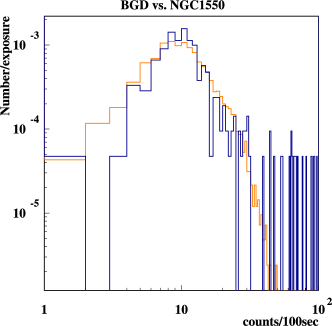
For the present purpose, an accurate background subtraction is of essential importance: in order to measure the ICM metallicity out to large radii where the X-ray surface brightness becomes low, we need to accurately determine not only atomic lines, but also contnuum. As template background files of the three EPIC detectors, we used those data taken with the medium filter, publicly released by the University of Birmingham group (Read and Ponman 2003). These background files are superpositions of multiple observations, and hence have higher statistics and smaller systematical errors than other background datasets currently available. These background events were rearranged to match the observational condition of NGC 1550, as originally developed with the ASCA GIS (Ishisaki 1995) and also applied to the XMM-Newton EPIC data by Kaastra et al. (2004). That is, we sorted the entire background data into subsets according to 100-sec averaged $10-12$ keV count rates, and created background spectra separately for individual subsets. We then combined them into a single background spectrum (one for each detector), using appropriate weights which are specified by the $10-12$ keV count rate histograms (averaged over 100 sec) of the actual NGC 1550 observation. For example, Figure 1 is the MOS1 $10-12$ keV count (per 100 sec) distribution during the NGC 1550 observation, compared with that of the template background. Thus, the two distributions are reasonably matched with each other. The background spectrum to be utilized in the present analysis, $B(E)$, is then synthesized as

$$B(E)=\frac{\Sigma\;T_{j}B_{j}(E)}{\Sigma\;T_{j}},$$ (1)

where $E$ is the energy, $T_{j}$ is the total residence time when the $10-12$ keV count is in the $j$-th interval, and $B_{j}(E)$ is the background template for the same $j$-th interval.

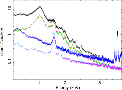
Katayama et al. (2004) studied the properties of the PN background and found that $2-7$ keV background rate correlates tightly with that in the $10-12$ keV band. Its correlation coefficient is 0.929, and the scatter around the correlation is less than 8%. Kaastra et al. (2004) showed that the MOS $0.2-10$ keV background flux scales proportionally to the $10-12$ keV background rate, and the spectral shape does not depend on the rate within an uncertaintly of 10%. Therefore, the above method of background synthesis is considered to reproduce the background with an accuracy better than 10%. Figure 2 compares the $0.5-9.0$ keV raw EPIC spectra of NGC 1550 with the estimated background spectra. In the higher energy range above $\sim 6$ keV, the two spectra agree within $10$% (1$\sigma$).

Since the Galactic absorption toward NGC 1550 is rather high as $1.15\times 10^{21}$ cm^-2 (Dickey & Lockman 1990), the cosmic X-ray background (CXB) which dominates the low energy band might be overestimated when the summed blank sky background is used. However, at 0.6 keV, the count rate ratios among the signal, particle background, and CXB is estimated to be $1:0.2:0.06$. If the Galactic absorption is $3\times 10^{20}$ cm^-2, this ratio becomes $1:0.2:0.09$. Therefore, the difference of the CXB level caused by using the averaged blank sky background is at most $\sim 3$% and $\sim 15$% of the signal and particle background at 0.6 keV, respectively. In order to deal with this uncertainty of cosmic X-ray background, and of the particle background as well, we put systematic errors to the spectra, following Kaastra et al. (2004). The systematic errors in the source spectrum were set at 5% in $0.5-2.0$ keV, and 10% above $2.0$ keV. To the background spectrum, we assigned errors of 25% in $0.5-0.7$ keV, 15% between $0.7-2.0$ keV, and 10% above 10 keV. We added these systematic errors in quadrature to the corresponding statistical errors.

3 X-ray Data Analysis and Results

3.1 Radial surface brightness

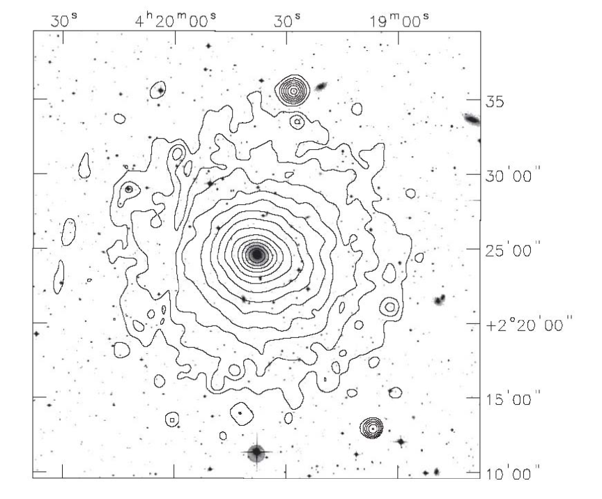
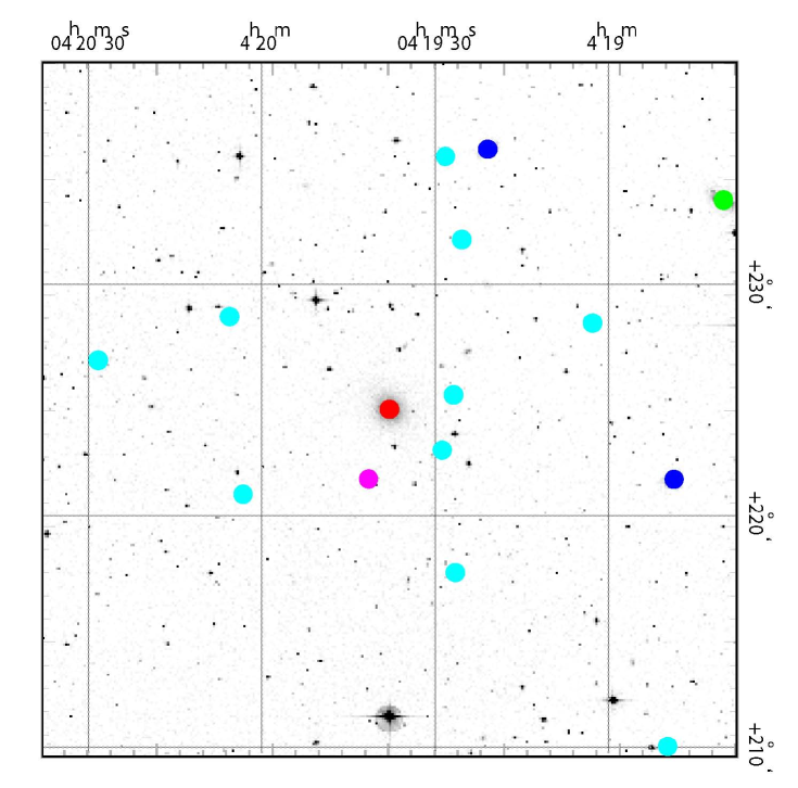
As shown in Figure 3 (left), the X-ray emission of NGC 1550 is spatially round, and extends at least up to a 2-dimensional radius of $b\sim 14^{\prime}\ (210\;$kpc$)$. The X-ray emission centroid coincides with the position of the NGC 1550 nucleus within $10^{\prime\prime}\;(\sim 3$ kpc). The signal-detected region is consistent with that obtained by ASCA (Paper I).

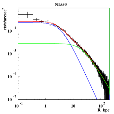
Figure 4 shows the azimuthally-averaged $0.5-4.5$ keV radial surface brightness profile $\Sigma(b)$, taken with MOS1 and presented after subtracting the blank-sky background as prepared above. We fitted the surface brightness profile by a $\beta$ model convolved with point-spread function (PSF). The position- and energy-dependence of the PSF was quoted from the XMM-Newton calibration note EPIC-MCT-TN_011 (Ghizzardi 2001). The single-$\beta$ model, however, did not reproduce the radial profile well, with $\chi^{2}/\nu=1446/599$ ($\beta=0.45$, and the core radius of $r_{\rm c}=5$ kpc). Therefore, we added another $\beta$ componet to the model as

$$\Sigma(b)=\Sigma_{1}\left\{1+\left(\frac{b}{r_{1}}\right)^{2}\right\}^{-3\beta_{1}+1/2}+\Sigma_{2}\left\{1+\left(\frac{b}{r_{2}}\right)^{2}\right\}^{-3\beta_{2}+1/2},$$ (2)

where $\Sigma_{1}$ and $\Sigma_{2}$ are normalization constants, while $r_{1}$ and $r_{2}$ are core radii. This “double-$\beta$” model has been successful, yielding $\chi^{2}/\nu=677/598$. The inner $\beta$ component is characterized by $\beta_{1}=0.60\pm 0.05$ and a core radius of $r_{1}=3\pm 1$ kpc, while those of the outer component are $\beta_{2}=0.50\pm 0.05$ and $r_{2}=20\pm 3$ kpc. These two components are shown separately in Figure 4.

In Paper I, a single-$\beta$ fit to the ASCA data was successful, and yielded $\beta=0.47\pm 0.01$ and $r_{\rm c}=16\pm 1$ kpc. The value of $\beta$ derived with ASCA is consistent with that of the outer $\beta$-component ($\beta_{2}$) obtained here, while the core radius of ASCA falls between $r_{1}$ and $r_{2}$ of XMM-Newton. We interpret that the angular resolution of ASCA was not sufficient to resolve the inner-$\beta$ component, which is seen within $\sim 15$ kpc or $\sim 1^{\prime}$.

According to Sun et al. (2003), the surface brightness profile of NGC 1550 obtained with Chandra cannot be reproduced by a single-$\beta$ model either, and requires a double-$\beta$ modeling. The derived outer component has $\beta=0.48$ and $r_{\rm c}\sim 26$ kpc, while the inner one is not described in their paper. Thus, the double-$\beta$ property, found with XMM-Newton, is also supported by the Chandra data. Sun et al. (2003) also found an excess emission within 1 kpc even above the double-$\beta$ fit; this is also suggested in our result, although the angular scale of 1 kpc, or $\sim 4^{\prime\prime}$, is comparable to the PSF of XMM-Newton.

3.2 Spectral analysis

In order to investigate global spectral properties of NGC 1550, we collected photons over a circular region of $14^{\prime}$ in radius from the galaxy nucleus. The background was subtracted in the same way as described in § 2, applying the same data integration region to the background dataset as the on-source data accumulation. The spectra obtained with the three EPIC detectors were fitted with an absorbed vMEKAL model (Kaastra & Mewe 1993) or an absorbed vAPEC model (Smith et al. 2001), using XSPEC 11.3.2. To secure a stable fit convergence to physically reasonable parameter values, we fixed abundances of He, C and N to one solar, constrained those of other metals from zero to 3 solar, and fixed the column density to the Galactic value ($1.15\times 10^{21}$ cm^-2). The employed energy range is $0.5-5.0$ keV for MOS, and $0.7-5.0$ keV for PN. The $0.5-0.7$ keV energy region of PN was excluded, because of systematic residuals below Fe-L lines often found in PN spectra of bright clusters (Tamura et al. 2004).

We have found that a reliable estimation of oxygen abundance requires a particular caution. This is because the oxygen K_α lines of NGC 1550 are weak, and the model continuum fitted over the $0.5-5.0$ keV range (or $0.7-5.0$ keV for PN) often becomes slightly ($\sim 5$%) higher (or lower) around the oxygen lines than the true continuum, probably due to calibration uncertainties. In this case, the oxygen abundance is forced to be lower (higher) than the true value with little allowance, because the overall model normalization is tightly constrained by the entire continuum and hence cannot vary freely. In fact, the oxygen abundance and the continuum normalization exhibit strong and negative coupling. In order to avoid this problem, we estimated the oxygen abundance by fitting the spectra over a limited energy range of $0.5-0.8$ keV, with all parameters except the oxygen abundance and the oxygen and continuum normalizations fixed to the best-fit values obtained through the full-band fitting. Although this would not be an orthodox method to evaluate a fitting parameter, it generally gives a more conservative and unbiased oxygen abundance.

We firstly fitted the spectra of the three EPIC detectors separately with a single temperature vAPEC model, in order to study systematic differences among the three EPIC detectors. The temperatures derived with PN, MOS1, and MOS2 are $kT=1.26_{-0.01}^{+0.01}\;{\rm keV}$, $1.28_{-0.01}^{+0.01}\;{\rm keV}$, and $1.28_{-0.01}^{+0.01}\;{\rm keV}$, respectively. The iron abundances from PN, MOS1, and MOS2 are $Z_{\rm Fe}=0.23_{-0.01}^{+0.01}\;{\rm solar}$, $0.26_{-0.02}^{+0.01}\;{\rm solar}$, and $0.25_{-0.02}^{+0.02}\;{\rm solar}$, respectively. Thus, the three EPIC detectors give consistent results within their statistical errors. In the following analysis, we therefore fit the specta of the three detectors simultaneously in order to improve the statistics.

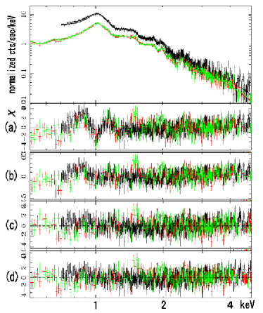
Figure 5 shows the results of the simultaneous fit using the vAPEC and vMEKAL models, and Table 1 summarizes the best-fit parameters. Although the obtained parameters are consistent with those derived with ASCA (Paper I), neither one-component model (vMEKAL or vAPEC) successfully reproduced the spectra. Since the fit residuals are seen around Fe-L line regions, a multi-temperature condition is suggested. Accordingly, we introduced a two-component model, consisting of two vAPEC (or vMEKAL) components with different free temperatures and normalizations. The two components are assumed to share the same metal abundances, and are subjected to the same Galactic absorption. Then, the fit has been improved and became acceptable (Figure 5c, 5d, and Table 1), with a $<$ 1% probability for this improvement to be accidental. We hereafter adopt the vAPEC code, because it can generally reproduce the Fe-L lines better (e.g. Matsushita et al. 2002); our results remain essentially the same even if we use the vMEKAL model. With the ASCA data, we derived the metal abundance to be $0.3\pm 0.1$ using the MEKAL model (Paper I). This is consistent with the iron and silicon abundances in Table 1, although the ASCA results are subject to larger errors.

Although we constrained the two vAPEC components to have the same metal abundances, this may not be necessarily warranted. Therefore, we tentatively relaxed this constraint, and found that the iron abundances of the hot and cool components became $Z_{\rm Fe,High}=0.34\pm 0.02$ and $Z_{f\rm Fe,Low}=0.43\pm 0.05$, respectively. Therefore, the tied value of $Z_{\rm Fe}=0.34\pm 0.01$ is considered to be appropriate for the hot component, while it may deviate from the true iron abundance of the cool component by $-20$%. Although this difference exceeds statistical errors, the fit is not improved significantly, because the F-test indicates a 88% probability of the difference by chance. Furthermore, the oxygen abundances became poorly constrained as $Z_{\rm O,High}=0.18\pm 0.07$ and $Z_{\rm O,Low}=0.71\pm 0.68$. Considering these, we retain our original assumption that the two vAPEC components share the same metal abundances. Even when taking into account the possible $\sim 20$% systematic error in the metal abundances of the cool component, our comparison between the metal distributions with that of the galaxy light, described in §5, remains essentially unaffected.

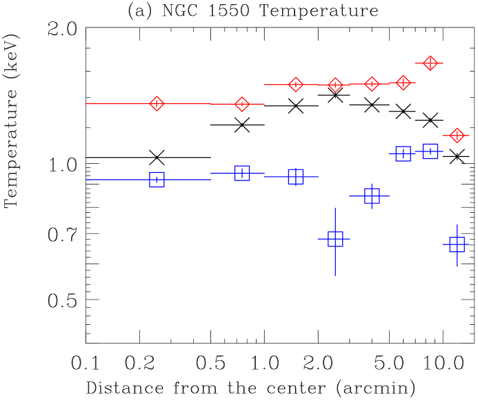
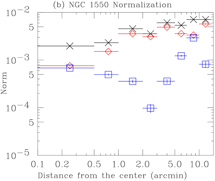
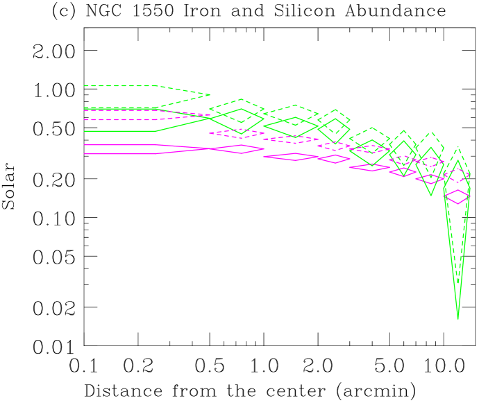
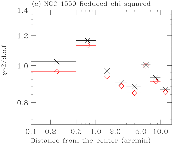
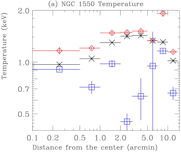
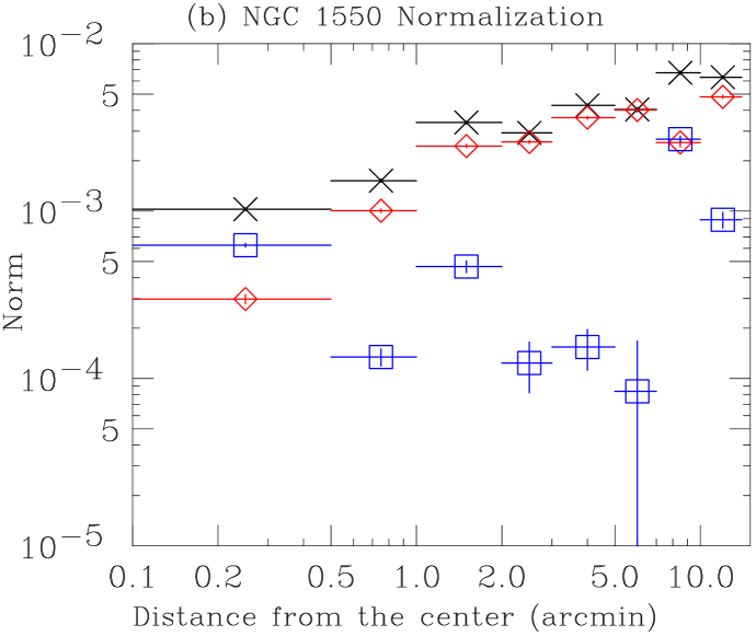
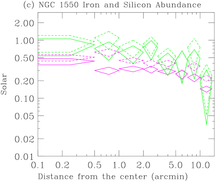
As a next step, we studied spatial variations of the temperature and metal abundances. For this purpose, we divided the image into eight concentric annular regions, centered on the X-ray emission peak (and hence on the central galaxy). The regions were chosen so that each of them contains more than 5,000 photons after the background subtraction. Then, the spectra of the eight regions were fitted in the same way as for the spatially integrated spectra. Figure 6 shows radial profiles of the temperature, abundances and the reduced chi-squared, derived by fitting the individual annular spectra (simultaneous among the three detectors) with one-temperature and two-temperature vAPEC models. The temperature determined with the one-component model increases mildly from 1.0 keV at the center to 1.4 keV at $\sim 3^{\prime}$ (45 kpc), and then returns to 1.0 keV at $\sim 10^{\prime}$ (150 kpc). Though somewhat depending on the modeling (single vs. double temperatures), the oxygen abundance is low and spatially rather constant, while those of the other metals clearly increase toward the center by a factor of 3 to 5. The iron and silicon profiles are rather similar, regardless of the temperature modeling, although the double-temperature fit yields systematically higher abundances than the single-temperature one. In all regions except for the outermost one, the two temperature model gives a better reduced chi-squared, and the $F$-test indicates that the probability of these improvements caused by chance is less than 1% in six regions except the $5.^{\prime}0-7.^{\prime}0$ and $10.^{\prime}0-14.^{\prime}0$ ones. The two temperatures (1.5 and 0.95 keV; Table 1) found with the region-integrated spectra can be understood reasonably as weighted means of the two temperatures specified by the eight annular spectra.

Although the EPIC data thus prefers the two-temperature modeling to the single-phase views, this could simply be due to projection effects. We accordingly deprojected the eight annular spectra into eight shell spectra using “onion-peeling” method (e.g. Buote et al. 2003), in which the contribution from the outer shell is subtracted progressively toward smaller radii. The emission from the region lying outside the outermost radius ($14^{\prime}$) was estimated by assuming that the spectrum of the outermost annulus extends with its surface brightness following the outer $\beta$ component derived in §3.1. In the model fitting to the deprojected spectra, we set initial parameter values to the best-fit ones obtained with the annular spectra, and again fixed or constrained the metal abundances in the same manner as the annular analysis. The obtained profiles of the model parameters, presented in Figure 7, are similar to those obtained from the annular spectra. The two modelings (single vs. two temperatures) are both acceptable essentially in all shells, and their fit goodness no longer shows the significant difference. This is due partially to the removal of the projection effects, and partially to reduced data statistics. Therefore, the plasma in each shell can be represented by a single-temperature collisionally-ionized plasma model, although local two-temperature (or multi-temperature) conditions are not necessarily ruled out.

4 Near Infra-Red Data Analysis

In order to estimate the galaxy light profile around NGC 1500, we utilezed the 2MASS (Two Micron All Sky Survey) data, which are accessible via NASA/IPAC Exgragalactic Database. In the 2MASS catalog, 33 galaxies (with $K$-band magnitude less than 14) have been found to be lying within $34^{\prime}$ of the NGC 1550 nucleus; at the distance of NGC 1550, this projected radius corresponds to 500 kpc. The sky positions of the galaxies in $30^{\prime}\times 30^{\prime}$ region around NGC 1550 are plotted in Figure 3 (right). Among the 33 galaxies, 7 galaxies listed in Table 2 are no fainter in $K$-band than NGC 1550 by 2.5 magnitude. These galaxies, except MCG+00-11-050 (of which the radial velocity is unknown), have radial velocities within $\pm 500$ km s^-1 of that of NGC 1550, and are likely to be members of the “NGC 1550 group”. Three galaxies (IC 0366, UGC 03011, and MCG+00-11-050) of the 7 are within the X-ray signal-detected region ($14^{\prime}$ in radius).

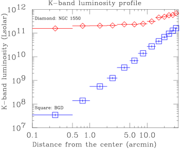
Figure 8 (red diamonds) shows the 2-dimensional integrated $K$-band profile around NGC 1550, constructed from NGC 1550 itself and the 33 galaxies. In this figure, the surface brightness profile of NGC 1550 is taken into account by using a public 2MASS background-subtracted $K$-band image of NGC 1550, while the other galaxies were treated as point sources. Since this profile must be contributed by background objects, we estimated the number of background galaxies expected in the $34^{\prime}$-radius region, based on the number counts of galaxies with $K\leq 14$ from the entire 2MASS sample (Bell et al. 2003). The $K$-band magnitude was converted to luminosity assuming the absolute $K$-band solar magnitude of 3.39 (Kochanek et al. 2001) and the same distance to all the galaxies as that to NGC 1550. Figure 8 (blue boxes) is the estimated two-dimensionally integrated background $K$-band luminosity profile. Even at the angular distance of $34^{\prime}$, the background is about 5 times lower than the integrated $K$-band luminosity of the NGC 1550 system. Within $34^{\prime}$ (510 kpc) and $14^{\prime}$ (210 kpc), the central galaxy carries $39$% and 70% of the background-subtracted $K$-band luminosity, respectively.

5 Spatial Distributions of Mass Components

5.1 Mass profiles

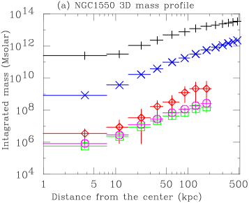
From the parameters of the X-ray emitting gas obtained in the spatial and spectral analyses (§3.1 and §3.2), we derived radially integrated mass profiles of three components constituting the NGC 1550 system; the ICM mass, the total mass, and the gaseous metal mass; the results are shown in Figure 9a. Below, we describe how these results have been obtained.

As a step to calculate the ICM mass profile, we started from the best-fit double-$\beta$ model of equation 2. We analytically deprojected it into a 3-dimensional emissivity profile as

$$\epsilon(r)=\epsilon_{1}\left\{1+\left(\frac{r}{r_{1}}\right)^{2}\right\}^{-3\beta_{1}}+\epsilon_{2}\left\{1+\left(\frac{r}{r_{2}}\right)^{2}\right\}^{-3\beta_{2}},$$ (3)

where $r$ is 3-dimensional radius from the emission centroid, and $\epsilon_{i}$ ($i=1,2$) are constants which are determined uniquely by $\Sigma_{i}$, $r_{i}$, and $\beta_{i}$ of equation (2). Then, the emissivity is rewritten as $\epsilon=\Lambda(T,Z)n_{\rm e}^{2}$, where $\Lambda(T,Z)$ is the cooling function specified by the measured temperature and metallicity, and $n_{\rm e}$ is the electron density. Using this $n_{\rm e}$, the ICM mass density profile is written as

$$\rho_{\rm gas}(r)=\mu m_{\rm p}n_{\rm e}(r)=\mu m_{\rm p}\sqrt{\frac{\epsilon(r)}{\Lambda(T,Z)}}\ \ .$$ (4)

Here $\mu=1.2$ is the mean molecular weight (i.e., the mean number of nucleon per electron). Values of $\Lambda(T,Z)$ were estimated for each shell region, utilizing $T$ and $Z$ measured in § 3.2, and referring to tables in Sutherland & Dopita (1993). Finally, we obtained the radially integrated ICM mass of Figure 9a, in the standard way, as

$$M_{\rm gas}(r)=\int_{0}^{r}\rho_{\rm gas}\ 4\pi r^{\prime 2}dr^{\prime}\ \ .$$ (5)

In Figure 9a, the gas mass profile outside $14^{\prime}$ was calculated assuming that the emissivity profile follows equation (3) with the same temperature and metal abundance as those in the $10^{\prime}$–$14^{\prime}$ region. In paper I, the ICM mass inside $r=220$ kpc was measured to be $3.4\times 10^{11}{\rm M}_{\odot}$; at the same radius, we now obtain a value as $M_{\rm gas}=7.6\times 10^{11}{\rm M}_{\odot}$. The difference is due to the inner $\beta$ component, which is apparent in Figure 4 and included in the XMM-Newton analysis. The ICM mass derived here is consistent with that from Chandra (Sun et al. 2003).

The metal mass density profiles in the ICM were derived by multiplying $\rho_{\rm gas}(r)$ of equation (4) with the measured metal abundances. For example, the radial profiles of the iron mass density, $\rho_{\rm Fe}(r)$, can be derived by multiplying the ICM mass profile with the iron abundance profile as

$$\rho_{\rm Fe}(r)=A_{\rm Fe}m_{\rm p}n_{\rm Fe}(r)=A_{\rm Fe}\left(\frac{n_{\rm Fe}}{n_{\rm H}}\right)_{\odot}\;Z_{\rm Fe}(r)\;f_{\rm H}\;\rho_{\rm gas}(r),$$ (6)

where $A_{\rm Fe}$ is the averaged atomic weight of Fe, $(n_{\rm Fe}/n_{\rm H})_{\odot}=4.68\times 10^{-5}$ is the number ratio of iron to hydrogen under one solar abundance (Anders & Grevesse 1989), $Z_{\rm Fe}(r)$ is the measured iron abundance, and $f_{\rm H}=0.75$ is the hydrogen mass fraction in the ICM. If another definition of solar abundance such as Grevesse & Sauval (1998) is adopted, $Z_{\rm Fe}(r)$ can change, but $\rho_{\rm Fe}(r)$ remains the same, because the change in $Z_{\rm Fe}(r)$ is canceled out by that in $\left(\frac{n_{\rm Fe}}{n_{\rm p}}\right)_{\odot}$; that is, $\rho_{\rm Fe}(r)$ is independent of the definition of the “solar abundance”. As to $Z_{\rm Fe}(r)$ in equation (6), we used the results from the single temperature fits to the deprojected shell spectra. However, as can be inferred from Figure 7c, the results do not change by more than 60% even when the two-temperature fits are employed.

At $r=210$ kpc, the integrated masses of iron, silicon, and oxygen imply $0.18^{+0.04}_{-0.05}$, $0.27^{+0.20}_{-0.13}$, and $0.29^{+0.54}_{-0.25}$ solar abundances, respectively, when divided by the integrated gas mass. In Figure 9a, iron and silicon exhibit very similar integrated mass profiles, reflecting similar abundance profiles (Figure 7c). In contrast, the integrated oxygen mass increases somewhat more steeply in Figure 9a than those of iron and silicon. Obviously, this is because the oxygen abundance is radially rather constant, unlike iron and silicon which show the central abundance enhancements. In a word, the oxygen mass profile is very similar to that of the ICM.

The integrated total mass profile was obtained assuming hydrostatic pressure equilibrium of the ICM in the gravitational potential, using the formula as

$$M_{\rm tot}(r)=-\frac{kTr}{\mu Gm}\left(\frac{d\ln{\rho_{\rm gas}}}{d\ln{r}}+\frac{d\ln{T}}{d\ln{r}}\right)\ \ ,$$ (7)

where $k$ is the Boltzmann constant and $G$ is the constant of gravity. In this calculation, the temperature $T$ refers to the values measured with the deconvolved spectra. We evaluated the term $\frac{d\ln{T}}{d\ln{r}}$ for each region by connecting two adjacent temperature points with a power-law, and substituting $\frac{d\ln{T}}{d\ln{r}}$ with the power-law slope averaged on both sides of each point. In the present case, $-\frac{d\;{\rm ln}\;\rho_{\rm gas}}{d\;{\rm ln}\;r}$ is in the range of $1.2{\bf-}2.1$, whereas $\frac{d\;{\rm ln}\;T}{d\;{\rm ln}\;r}$ is typically $\lesssim 0.1$ (0.5 at maximum). Therefore, the proper inclusion of the $\frac{d\;{\rm ln}\;T}{d\;{\rm ln}\;r}$ term reduces the estimated $M_{\rm tot}$ up to several tens percent, in those regions where $T(r)$ is increasing outward. Outside $14^{\prime}$, the temperature was assumed to be radially constant and the same as that in the $10^{\prime}$–$14^{\prime}$ region. At $r\sim 210$ kpc, we thus obtain the total mass as $2.0\times 10^{13}M_{\odot}$, which agrees with the value of $2\times 10^{13}M_{\odot}$ typically found among galaxy groups (Mulchaey et al. 1996). Also, the present result agrees with that in Paper I; $1.6\times 10^{13}M_{\odot}$ at $r=210$ kpc. The total mass profile obtained with Chandra (Sun et al. 2003) is consistent with our profile (Figure 9a) within respective errors. Furthermore, the gas-mass fraction at $\sim 400$ kpc (half the virial radius), $M_{\rm gas}/M_{\rm tot}=0.06$, is consistent with those observed from galaxy groups at a radius of overdensity $\sim 500$ (Vikhlinin et al. 2006).

Based on ASCA observation, Dupke & Bregman (2005) reported the presence of a velocity difference by $\geq 1.5\times 10^{3}$ km s^-1 in the ICM of NGC 1550. If so, equation (7), which assumes hydrostatic confinement of the ICM, would become no longer valid. However, a claimed velocity difference of $2400\pm 1000$ km $s^{-1}$ in the Centaurus cluster, by the same authors (Dupke & Bregman 2006), was not found significantly by the latest Suzaku measurements, with an upper limit velocity of $1400$ km s^-1 at 90% confidence range (Ota et al. 2007). Therefore, the reality of the reported bulk motion in the ICM of NGC 1550 is open, and hence we retain our original assumption of hydrostatic equilibrium. Even if the bulk motion is real, the total mass estimate would change only by a factor of $\sim 2$ (Ota et al. 2007), which does not affect our main results.

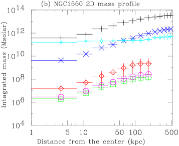
The present study requires a quantitative comparison of the X-ray derived 3-dimensional radial mass profiles against visible-light distribution representing the stellar mass profile. However, the galaxy distribution obtained in §4 is a 2-dimensional quantity expressed on the celestial sphere. Therefore, we have to deproject the galaxy profile into three dimensions, or alternatively, project the other three-dimensional profiles (the total mass, gas mass, and metal masses) onto two dimensions. We have adopted the latter method, because the galaxies aroung NGC 1550 are too sparsely distributed to allow reliable deprojection. Figure 9b shows the projected mass profiles in the integrated form, including the galaxy mass profile. In the derivation of the galalxy masses, we assumed $K$-band stellar mass-to-light ratio ($M/L$) of all the galaxy to be 1.0 for simplicity, altough $M/L$ in $K$-band varies approximately between 0.5 and 1.0 according to the color of galaxies (Bell et al. 2003). Thus, the galaxy mass profile presented here is essentially the same as the $K$-band luminosity profile.

As can be seen in Figure 9b, the radially-integrated $K$-band mass-to-light ratio of the system reaches $75\pm 3\;M_{\odot}/L_{\odot}$ at 210 kpc. Considering a typical color of galaxies, this value is consistent with the $B$-band mass-to-light ratio of $\sim 380\;M_{\odot}/L_{\odot}$ ($r<210$ kpc) derived in Paper I. These values are comparable to those of clusters of galaxies. In fact, the mass-to-light ratio of galaxy clusters is typically measured to be $\sim 250\;M_{\odot}/L_{\odot}$ in $B$-band (Bartelmann & White 2002) and $\sim 80\;M_{\odot}/L_{\odot}$ in $K$-band (Kochanek et al. 2003).

5.2 Iron-mass-to-light ratio profile

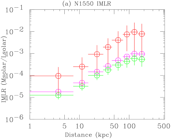
As shown by Figure 9b, the ICM distribution is slightly more extended than that of the total mass (i.e. the gas fraction increasing toward the cluster outskirts), in agreement with previous reports (e.g. Markevitch & Vikhlinin 1997). Furthermore, the figure clearly reveals that the integrated stellar luminosity profile is significantly flatter than the other profiles: the stellar component is much more concentrated than the other components. The difference between the stellar luminosity profile and those of the metal masses is particularly interesting, because the metals should have originated from stars. In order to see the difference more clearly, we divided the integrated iron mass profile by integrated $K$-band luminosity profile, to obtain so-called iron-mass-to-light ratio (IMLR) profile (Finoguenov 2000). The radially-integrated IMLR profile of NGC 1550, shown in Figure 10a, drops toward the center by about two orders of magnitudes, while flattens outside $\sim 100$ kpc. This behavior is in agreement with the $ASCA$ result on the Centaurus cluster and Abell 1060 (Makishima et al. 2001), suggesting that the IMLR decreases towards the center are common among regular clusters regardless of their richness. The silicon-mass-to-light ratio (SiMLR) and oxygen-mass-to-light ratio (OMLR) profiles also decrease toward the center to the same degree as the IMLR.

5.3 Density-density plot

The IMLR and similar quantities compare two relevant mass components in the form of ratios between their radially-integrated profiles. This approach is useful to grasp large-scale behavior of these components, but may not be suitable to investigate more localized features. For this purpose, we devised a new plot which we named density-density plot (DDP). A DDP plots densities of a component in individual shells against those of another component in the corresponding shells. Although the spatial coordinate is lost in a DDP, we can directly see the relation between any two mass components in their differential forms.

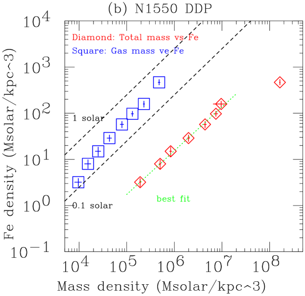
Figure 10b shows DDPs between the total mass and iron mass (red diamonds), and between the gas mass and iron mass (blue squares). The latter DDP indicates that the iron mass density increases (toward the center) somewhat more steeply than the ICM mass density, just reflecting the iron abundance increase in Figure 7c from $\sim 0.15$ solar at $r\sim 200$ kpc to $\sim 0.5$ solar at the center.

Interestingly, we instead find in Figure 10b a very good proportionality between the iron mass density and the total gravitating mass density (red diamonds) except at the very center. In fact, the least-square fit with a power law function yields the best relation between these two quantities, excluding the innermost data point, as

$$\rho_{\rm Fe}=(3.2\pm 1.6)\times 10^{-5}\;\rho_{\rm tot}^{0.95\pm 0.03},$$ (8)

while the relation between the iron mass density and the ICM mass density becomes

$$\rho_{\rm Fe}=(4.7\pm 3.3)\times 10^{-5}\;\rho_{\rm ICM}^{1.24\pm 0.09}.$$ (9)

In other words, the iron in the ICM traces the total mass distribution (except the innermost region) rather than that of the ICM density. In the innermost region ($r<7.5$ kpc), the iron mass fraction decreases significantly relative to the total mass. This is likely to be related to the dominance of the stellar mass of NGC 1550 in this region, although it is not immediately clear, at this stage, why the iron mass increases less prominently than the stellar mass.

Incidentally, equation (8) and equation (9) can be combined into a relation between the ICM mass density and the total mass density, as $\rho_{\rm ICM}\propto\rho_{\rm tot}^{0.77\pm 0.08}$. This is reasonable, because the index of 0.77 is close to the typical value of $\beta\sim 0.7$ (Mohr et al. 1999) found among clusters, where $\beta$ is the same index as employed in equation (2).

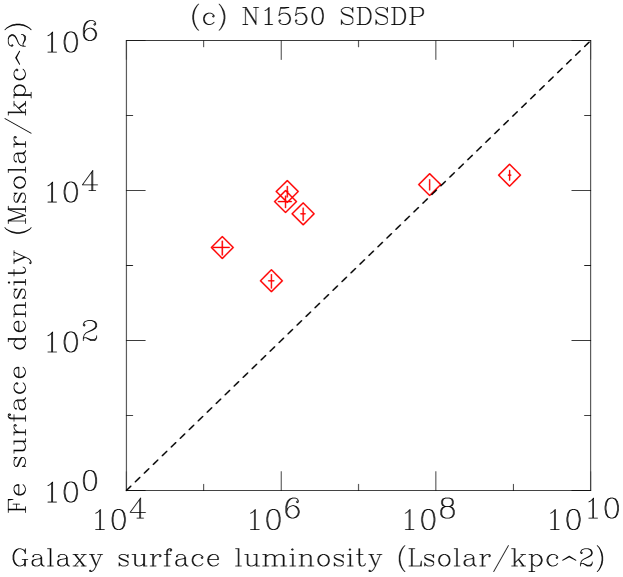
In order to investigate the above issue at the innermost region, let us compare densities between the galaxy $K$-band luminosity and the iron mass. For the same reason as described in §5.1, we use the 2-dimensional form, which we named Surface Density-Surface Density Plot (SDSDP): a SDSDP plots the surface density of a component in the individual 2-dimensional annular regions against those of another component. Figure 10c shows a SDSDP between the galaxy $K$-band luminosity ($\Sigma_{\rm gal}$) and the iron mass ($\Sigma_{\rm Fe}$). Thus, the innermost two regions having $>10^{8}L_{\odot}$ kpc^-2 are more optically luminous than the other regions by $\sim 2$ orders of magnitude. This demonstrates the characteristic of the NGC 1550 system as an IXEG. In contrast, the iron surface density does not exhibit such a steep increase to the center, so that $\Sigma_{\rm Fe}$ is not proportional to $\Sigma_{\rm gal}$ particularly toward the center. This is another expression of the IMLR profile (Figure 10a): in the central region of the NGC 1550 system, iron in the ICM becomes much depleted relative to the stellar light, even though it moderately increases relative to the ICM mass density.

As can be readily inferred, the relation between silicon and the stellar mass is essentially the same as that between iron and the stars. Oxygen (though not shown) is even more depleted in the central region than iron and silicon, because it lacks the central abundance increase.

6 Discussion

Using the XMM-Newton EPIC and 2MASS $K$-band data, we derived the radial profiles of components constituting the NGC 1550 system; the gas mass, total mass, metal mass, and the galaxy luminosity. As seen in Figure 7c and Figure 9, the metals (oxygen, silicon, and iron) are extended to $\sim 200$ kpc from the center, wherein $\sim$ 70% of the $K$-band luminosity is carried by NGC 1550 itself. Most importantly, we have found that iron (as well as silicon) in the ICM traces very well the total gravitating mass (eq. [7]), whereas the stellar component is significantly more concentrated to $r<15$ kpc. This is a non-trivial result, since we would naturally expect the metals to trace the stellar mass unless at least either of them evolved significantly over the Hubble time in the radial distribution.

The above finding allows three alternative scenarios; one is that the iron within $\sim 100$ kpc has been transported outwards; another is that iron in the central region is contained in the central galaxy and hidden from our X-ray view. The other is that the galaxies have gradually concentrated toward the center (particularly onto NGC 1550) while supplying metals to the surrounding hot gas.

In the first scenario, metals in the central region must have been transported outward, together with the ICM (mostly hydrogen and helium), through diffusion or bulk outflow. As discussed in Ezawa et al. (1997; 2001), the diffusion constant $D$ of iron in the hot gas is given as

$$D=2\times 10^{26}\left(\frac{n_{\rm e}}{10^{-4}\;{\rm cm}^{-3}}\right)^{-1}\left(\frac{kT}{3\;{\rm keV}}\right)^{5/2}{\rm cm}^{2}\;{\rm s}^{-1}.$$ (10)

Therefore, the iron atoms in the ICM can diffuse at most $\sim 10$ kpc over the Hubble time; this is by far insufficient to explain the present results. In the case of bulk outflow, a large amount of hot gas within 100 kpc, comparable in mass to what presently exists there, must have been evacuated to realize the IMLR of Figure 10a and SDSDS of Figure 10c. Since the mass of the hot gas within $100$ kpc is $6\times 10^{11}M_{\odot}$ (Figure 9b), the outflow rate becomes $\sim 50\;M_{\odot}{\rm yr}^{-1}$ if we assume a constant rate over the Hubble time. This is just opposite to the case of cooling flows. In other words, the energy needed to drive out the central ICM must have been large enough to reverse cooling flows. However, even among medium-richness clusters, it is generally considered non-trivial to find an energy source which is strong enough to suppress cooling flows of this order (e.g. Makishima et al. 2001). Since the depth of gravitational potential is comparable to the velocity dispersion of galaxies $\sigma_{\rm gal}$, the energy required to evacuate the central ICM, $E_{\rm eva}$, becomes enormous, as

$$E_{\rm eva}\sim M_{\rm eva}\sigma_{\rm gal}^{2}=3\times 10^{60}\left(\frac{\sigma_{\rm gal}}{400\;{\rm km}\;{\rm s}^{-1}}\right)^{2}\;{\rm erg}.$$ (11)

where $M_{\rm eva}\sim 1\times\;10^{12}M_{\odot}$ is a typical ICM mass to be evacuated.

The most popular candidate for driving the outflow is activity of the central galaxy nucleus. Actually, NGC 1550 hosts a weak radio source of which the flux density is $16.6\pm 1.6$ mJy at 1.4 GHz (Condon et al. 1998). However, for the estimated kinetic energy (power times age) provided by an AGN to become comparable to equation (11), the object needs to be as strong a radio source as Cygnus A (e.g. Kino et al. 2005); the present radio luminosity of the NGC 1550 nucleus falls 6 orders of magnitude in short. Of course, we cannot exclude an extreme possibility that the nucleus remained highly active (either continuously or intermittently) till a near past, and then declined at present. In such a case, we would observe large ($\sim 100$ kpc) cavities in the ICM, but there is no such evidence. Alternatively, the radiation pressure from the AGN may have caused the outflow. If we assume the ICM within 100 kpc from the center has been pushed away, the luminosity of the AGN has to be

$$L_{\rm AGN}=\left(\frac{\dot{E}_{\rm eva}}{\tau_{\rm T}}\right)=4\times 10^{46}\;{\rm erg}\;{\rm s}^{-1},$$ (12)

where $\dot{E}_{\rm eva}$ is the evacuation power averaged over the Hubble time, and $\tau_{\rm T}=2\times 10^{-4}$ is the cross section for Thomson scattering. It is unlikely that the NGC 1550 nucleus has been so luminous for the Hubble time. Yet another weak point of the scenario is that it needs some fine tuning mechanisms to make $\rho_{\rm Fe}$ proportional to $\rho_{\rm tot}$ as indicated by equation (7) and the DDP of Figure 10b. Thus, the bulk outflow scenario is also unlikely.

The second scenario assumes that the IMLR decreases toward the center because a significant fraction of iron in the central region has been taken inside the stars in NGC 1550, thus increasing the stellar metallicity of NGC 1550 compared to those of the other peripheral galaxies. This “hidden”amount of iron becomes comparable to that in the hot gas within 100 kpc, that is, $2\times 10^{8}M_{\odot}$ (Figure 9b). For comparison, the stellar mass in NGC 1550 is estimated to be $2\times 10^{11}M_{\odot}$, assuming again the $K$-band stellar mass-to-light ratio to be 1. Therefore, the hidden iron should increase the mean stellar metal abundance by $\sim 0.5$ in solar units. In this estimate, we can ignore the amount of iron confined in interstellar matter (ISM) in these galaxies, because the mass of ISM is at most 10% of the stellar mass (Matsushita 2000). From a color-metallicity relation studied by Barmby et al. (2000), the stellar metallicity of NGC 1550 is estimated to be $0.5-0.7$ solar abundance, using $U$,$B$,$V$,$J$, and $K$ magnitude. On the other hand, Jordán et al. (2004) showed that the metallicity of early-type galaxies correlates well with the absolute magnitude $M_{V}$. From this correlation, the metallicity of galaxies having the same $M_{V}$ as NGC 1550 is estimated as $\sim 0.8$ solar. Since this is not much different from the value estimated from the color of NGC 1550, there is no reason to presume that NGC 1550 has locked a much larger fraction of its metal products into its stars than other elliptical galaxies with simillar $V$-band luminosities.

The remaining scenario assumes gradual concentration, or infall, of the member galaxies toward the system center. This view is suggested by the present and other (e.g., Makishima et al. 2001) results, that the stellar mass in groups and clusters are generally much more concentrated, not only than the metals in the ICM, but also than the ICM itself and the total mass (Figure 9b). The former two scenarios would not easily explain these differences among the metals, stars, and the total mass (dominated by the dark matter). To be more quantitative, let us assume, as a simplest case, that the system initially consisted mainly of $\sim 10$ galaxies each with $K\sim 11$, which is comparable to IC 0366 but an order of magnitude less luminous than the present-day NGC 1550. If only one of them was initially at $r\lesssim 50$ kpc while the others were outside, the IMLR at this radius was initially an order of magnitude higher than it is at present, and hence the IMLR profile at that time was approximately flat as would be naturally expected. If these galaxies have all merged into the central single galaxy (i.e., the present-day NGC 1550) after their metal supply was mostly over, we can explain both its present optical luminosity, and the central decrease in the IMLR profile. In other words, NGC 1550 is indeed suggested to be a remnant of such a merger process, as implied by the nomenclature of “fossil group” (Jones et al. 2003).

As to the mechanism which drives the suggested galaxy infall, a promising candidate is dynamical pressure exerted onto galaxies when they swim through the ICM. According to Sarazin (1988), this effect will cause the kinetic energy $K$ of a galaxy, moving with a velocity $v$, to decrease at a rate of

$$dK/dt=-\pi\rho_{\rm gas}v^{3}R_{\rm int}^{2}~{}~{},$$ (13)

where $R_{\rm int}$ is “interaction radius” with which the galaxy interacts with the ICM and displaces it. Then, the galaxy will lose its kinetic energy on a time scale of

$$\tau\equiv\frac{K}{|dK/dt|}=\frac{m_{\rm gal}}{2\pi\rho_{\rm gas}vR_{\rm int}^{2}}~{}~{},$$ (14)

where $m_{\rm gal}$ is the galaxy mass.

As discussed by Makishima et al. (2001), the value of $R_{\rm int}$ is estimated to be comparable to the visual galaxy size, because the in-flowing ICM will be intercepted by magnetic fields anchored to the galaxy. Assuming hence $R_{\rm int}=10$ kpc, and employing plausible values for the other parameters, equation (14) yields

$$\tau=14\left(\frac{m_{\rm gal}}{1\times 10^{11}M{{}_{\odot}}}\right)\left(\frac{n_{\rm gas}}{10^{-3}\;{\rm cm^{-3}}}\right)^{-1}\left(\frac{v}{400\;{\rm km\;s^{-1}}}\right)^{-1}\left(\frac{R_{\rm int}}{10\;{\rm kpc}}\right)^{-2}~{}{\rm Gyr}$$ (15)

which is of the same order as the Hubble time. Then, the galaxies moving in dense ICM will fall toward the center, merge together, and change their morphology (Makishima et al. 2001), on the Hubble time scale. Importantly, equation (15) predicts less massive galaxies to fall more rapidly (on condition that $R_{\rm int}$ depends only weakly on $m_{\rm gal}$), in agreement with the idea that small galaxies which may have existed in the system have mostly merged into NGC 1550. This mass dependence is opposite to that of the gravitational dynamical friction, which works among galaxies moving in vacuum and causes more massive galaxies to sink to the potential center.

The scenario described above is not considered specific to the NGC 1550 system, since the dynamical pressure cannot be avoided as long as galaxies are moving through the ICM. Employing the empirical relation among the cluster mass $M$, the X-ray luminosity $L_{\rm x}$, and the temperature $T$ as $L_{\rm x}\propto T^{3}$ and $M\propto T^{3/2}$ (e.g. Arnaud et al. 2005), The ICM density $n_{\rm gas}$ in a cluster is found to scale as $\propto T^{1/2}$; here we also utilized the virial relation as $M/R\propto T$, and the luminosity relation as $L_{\rm x}\propto n_{\rm gas}^{2}R^{3}T^{1/2}$, where $R$ is the cluster radius. Then, with $v\propto T^{1/2}$, equation (14) predicts $\tau\propto T^{-1}$, so that richer systems are expected to have somewhat shorter merging time scales. In fact, the central decrease in the IMLR profile has been observed from richer systems as well (Finoguenov et al. 2000; Makishima et al. 2001; Kawaharada 2006), including the Centaurus cluster and Abell 1060. Interestingly, in Figure 9 of Finoguenov et al. (2000), the IMLR profiles in HCG 51 and HCG 62 are flatter than those of the other groups and clusters. This support the galaxy-infall scenario indirectly, because a compact group is considered to be a galaxy group in which galaxy mergers are proceeding. Furthermore, the ICM dynamical pressure might also explain some evolutionary effects observed from rich clusters, such as the long-known Butcher-Oëmler effect (Butcher & Oëmler 1978), and the significant evolution of galaxy morphology in dense cluster environments (e.g., van Dokkum et al. 2000; Goto 2005).

It is known that galaxy groups exhibit rather large scatter in their gas richness (Osmond & Ponman 2004), with spiral-rich ones tending to be particularly gas poor (Ota et al 2004). From equation (15), we may then speculate that a galaxy group borne as a relatively gas-rich system is subject to a fast merger process, while it remains otherwise an ordinary group. If this view is correct, an IXEGs could be a system in which baryons remained for some reason mostly in the hot gas phase, with a relatively lower galaxy mass. The NGC 1550 system agrees with this view, because it is as gas-rich as ordinary galaxy groups in terms of the gas-to-total mass ratio (Paper I), while it is optically comparable to a single galaxy.

Table 1: Results of the model fitting to the MOS and PN spectra within $14^{\prime}$ of the NGC 1550 nucleus.

			abundances (solar)
Model	Temperature (keV)	Ratio	Fe	Si	O	$\chi^{2}/$dof
vMEKAL	$1.32\pm 0.01$	–	$0.29\pm 0.01$	$0.31\pm 0.02$	$0.13\pm 0.03$	2012/1423 = 1.41
vAPEC	$1.27\pm 0.01$	–	$0.24\pm 0.01$	$0.32\pm 0.02$	$0.13\pm 0.03$	1813/1425 = 1.27
2vMEKAL	$1.50\pm 0.02$ / $0.87\pm 0.01$	5.91	$0.42\pm 0.01$	$0.45\pm 0.02$	$0.24\pm 0.04$	1640/1421 = 1.15
2vAPEC	$1.48\pm 0.02$ / $0.95\pm 0.01$	4.08	$0.34\pm 0.01$	$0.40\pm 0.02$	$0.18\pm 0.03$	1666/1423 = 1.17

Table 2: Major candidate of member galaxies in the NGC 1550 system.

Name	$\Delta\theta$ (arcmin)	$K$ (mag)	$v_{r}$ (km s-1)
NGC 1550	0	8.774	3714
IC 0366	3.1	11.104	3736
UGC 03011	12.0	10.891	4207
MCG+00-11-050	12.7	10.840	–
UGC 03008	17.0	9.687	3251
CGCG 393-007	17.1	10.308	3912
CGCG 393-008	23.6	9.955	3973
UGC 03006	33.2	9.581	3664

Figure 1: MOS1 $10-12$ keV count-rate histograms of the NGC 1550 observation (dark blue) and the template background (orange) with 100 sec integration, both normalized to their exposures.

Figure 2: $0.5-9.0$ keV Raw spectra of PN (black), MOS1 (red), and MOS2 (green) extracted from the $0^{\prime}-14^{\prime}$ region. For comparison, estimated background spectra of PN (blue), MOS1 (cyan), and MOS2 (magenta) are also plotted.

Figure 3: (left) The $0.5-4.5$ keV EPIC MOS1 surface brightness (contours) of NGC 1550, including background, overlaid on an optical image of Digitazed Sky Survey (greyscale) plotted on J2000 ($\alpha$, $\delta$) coordinates. The X-ray image is smoothed by a gaussian filter with $\sigma=20^{\prime\prime}$, but not corrected for vignetting. The contours are logarithmically spaced, with a step of factor 1.4. (right) The same optical image of Digitazed Sky Survey as left panel, where also plotted are positions of galaxies around NGC 1550 identified in the 2MASS catalog. Colors specify their $K$-band magnitudes as $8<K<9$ in red, $9<K<10$ in green, $10<K<11$ in blue, $11<K<12$ in magenta, and $13<K$ in cyan. Galaxies with $12<K<13$ are not present in this sky region.

Figure 4: The $0.5-4.5$ keV background-subtracted and vignetting-corrected X-ray surface brightness of NGC 1550 created with the MOS1 data (black crosses), shown together with the best-fit double-$\beta$ model (red). The data were azimuthally averaged around the NGC 1550 nucleus. The constituent two $\beta$ components are shown in blue and green.

Figure 5: Response-inclusive $0.5-5.0$ keV PN (black), MOS1 (red) and MOS2 (green) spectra from the $0^{\prime}-14^{\prime}$ region, simultaneously fitted with; (a) an absorbed vMEKAL model, (b) an absorbed vAPEC model, (c) a two-temperature vMEKAL model, and (d) a two-temperature vAPEC model. In the two temperature fits, the metal abundances are tied between the two components, while the temperatures and normalizations are left free.

Figure 6: Radial profiles of the X-ray spectroscopic parameters, derived with 8 annular spectra. (a) The temperature derived with the single (black) and double (red and blue) vAPEC fits. (b) The vAPEC normalizations (proportional to emission measure), with the same color definitions as in panel (a). (c) The iron (magenta) and silicon (green) abundances obtained from the single (solid diamonds) and double (dashed diamonds) vAPEC fits. (d) The oxygen abundances, with the same definitions of solid and dashed diamonds as (c). (e) The reduced chi-squared from the single (black) and double (red) vAPEC fits.

Figure 7: The same as Figure 6, but for the deprojected spectra.

Figure 8: A two dimensionally integrated $K$-band luminosity profile around NGC 1550 (red diamonds), compared with that of the estimated field galaxies (blue squares). The latter is calculated assuming that all the galaxies are at the same distance as NGC 1550.

Figure 9: Integrated radial profiles of various mass components in the NGC 1550 system, shown in 3-dimensional forms (panel a) and projected forms (panel b). Black crosses indicate the total mass calculated by equation (7), while blue crosses the total gas mass obtained by equation (5). Small cyan diamonds are the galaxy mass derived in §4, shown only in the projected form. Metals in the gas are specified by colors; O (red diamonds), Si (green squares), and Fe (magenta circles).

Figure 10: (a) Radially-integrated $K$-band iron-mass-to-light (magenta), silicon-mass-to-light (green), and oxygen-mass-to-light (red) ratio profiles of NGC 1550. For convenience, the angular separation is converted to physical distance, assuming that all the galaxies are at the same distance as NGC 1550. (b) Density-density plots between the total mass and iron mass (red diamonds), and between the gas mass and iron mass (blue squares). Two dashed lines indicate 0.1 and 1.0 solar abundances of the iron mass. Green dotted line shows the best fit power-law relation between the iron density and the total mass density, $\rho_{\rm Fe}=3.191\times 10^{-5}\;\rho_{\rm tot}^{0.947}$, excluding the innermost data point. (c) A surface density-surface density plot between the galaxy $K$-band luminosity and iron mass (red diamonds). The dashed line represents $\Sigma_{\rm Fe}\propto\Sigma_{\rm gal}$ for reference.

References

- anders (1989) Anders, E., & Grevesse, N. 1989, GeCoA, 53, 197
- arnaud (2005) Arnaud, M., Pointecouteau, E., & Pratt, G. W. 2005, A&A, 441, 893
- barmby (2000) Barmby, P., & Huchra, J. P. 2000, ApJ, 531, L29
- barnes (1989) Barnes, J. 1989, Nature, 338, 123
- bartelmann (1989) Bartelmann, M., & White, S. D. M. 2002, A&A, 388, 732
- bell (2003) Bell, E. F., McIntosh, D. H., Katz, N., & Weinberg M. D. 2003, ApJS, 149, 289
- buote (2003) Buote, D. A., Lewis, A. D., Brighenti, F., & Mathews W. G. 2003, ApJ, 594, 741
- butcher (1978a) Butcher H., & Oemler A. Jr. 1978, ApJ, 219, 18
- butcher (1978b) Butcher H., Oemler A. Jr. 1978, ApJ, 226, 559
- condon (1988) Condon, J. J., Cotton, W. D., Greisen, E. W., Yin, Q. F., Perley, R. A., Taylor, G. B., & Broderick, J. J. 1998, AJ, 115, 1693
- dariush (2007) Dariush, A., Khosroshahi, H. G., Ponman, T. J., Pearce, F., Raychaudhury, S., & Hartley, W. 2007, MNRAS, 382, 433
- dicky (1990) Dickey, J. M., & Lockman, F. J. 1990, ARA&A, 28, 215
- d’onghia (2005) D’Onghia, E., Sommer-Larsen, J., Romeo, A. D., Burkert, A., Pedersen, K., Portinari, L., & Rasmussen, J. 2005, ApJ, 630, L109
- dupke (2005) Dupke, R. A., & Bregman, J. N. 2005, ApJS, 161, 224
- dupke (2006) Dupke, R. A., & Bregman, J. N. 2006, ApJ, 639, 781
- ezawa (1997) Ezawa, H., Fukazawa, Y., Makishima, K., Ohashi, T., Takahara, F., Xu, H., & Yamasaki N. Y. 1997, ApJ, 490, L33
- ezawa (2001) Ezawa, H., Yamasaki, N. Y., Ohashi, T., Fukazawa, Y., Hirayama, M., Honda, H., Kamae, T., Kikuchi, K., & Shibata R. 2001, PASJ, 53, 595
- finoguenov (2000) Finoguenov, A., David, L. P., & Ponman, T. J. 2000, ApJ, 544, 188
- ghizzardi (2001) Ghizzardi, S. 2001, in IN FLIGHT CALIBRATION OF THE PSF FOR THE MOS1 AND MOS2 CAMERAS, XMM-Newton Calibration note EPIC-MCT-TN-011, 22
- grevesse (1998) Grevesse, N., & Sauval, A. J. 1998, SSRv, 85, 161
- goto (2005) Goto T. 2005, MNRAS, 359, 1415
- ishisaki (1995) Ishisaki, Y. 1995, Ph.D. Thesis, The University of Tokyo
- jones (2003) Jones, L. R., Ponman, T. J., Horton, A., Babul, A., Ebeling, & H., Burke, D. J. 2003, MNRAS, 343, 627
- jordan (2004) Jordán, A., Côté, P., West, M. J., Marzke, R. O., Minniti, D., & Rejkuba, M. 2004, AJ, 127, 24
- kaastra (1993) Kaastra, J. S., & Mewe, R. 1993, A&AS, 97, 443
- kaastra (2004) Kaastra, J. S., Tamura, T., Peterson, J. R., Bleeker, J. A. M., Ferrigno, C., Kahn, S. M., Paerels, F. B. S., Piffaretti, R., Branduardi-Raymont, G., & Böhringer, H. 2004, A&A, 413, 415
- katayama (2004) Katayama, H., Takahashi, I., Ikebe, Y., Matsushita, K., & Freyberg, M. J. 2004, A&A, 414, 767
- kawaharada (2003) Kawaharada, M., Makishima, K., Takahashi, I., Nakazawa, K., Matsushita, K., Shimasaku, K., Fukazawa, Y., & Xu H. 2003, PASJ, 55, 573
- kawaharada (2006) Kawaharada, M. 2006, Ph.D. Thesis, The University of Tokyo
- khosroshahi (2007) Khosroshahi, H. G., Ponman, T. J., & Jones, L. R. 2007, MNRAS, 377, 595
- kino (2005) Kino, M., & Kawakatu, N. 2005, MNRAS, 364, 659
- kochanek (2001) Kochanek, C. S., Pahre, M. A., Falco, E. E., Huchra, J. P., Mader, J., Jarrett, T. H., Chester, T., Cutri, R., et al. 2001, ApJ, 560, 566
- kochanek (2002) Kochanek, C. S., White, M., Huchra, J., Macri, L., Jarrett, T. H., Schneider, S. E., & Mader, J. 2003, ApJ, 585, 161
- kodama (2000) Kodama, T., & Matsushita, K. 2000, ApJ, 539, 149
- makishima (2001) Makishima, K., Ezawa, H., Fukuzawa, Y., Honda, H., Ikebe, Y., Kamae, T., Kikuchi, K., Matsushita, K., et al. 2001, PASJ, 53, 401
- markevitch (1997) Markevitch, M., & Vikhlinin, A. 1997, ApJ, 491, 467
- matsushita (1998) Matsushita, K., Makishima, K., Ikebe, Y., Rokutanda, E., Yamasaki, N., Ohashi, T. 1998, ApJ, 499, L13
- matsushita (2000) Matsushita, K., Ohashi, T., & Makishima, K. 2000, PASJ, 52, 685
- matsushita (2001) Matsushita, K. 2001, ApJ, 547, 693
- matsushita (2002) Matsushita, K., Belsole, E., Finoguenov, A., & Böhringer, H. 2002, A&A, 386, 77
- matteucci (1988) Matteucci, F., & Vettolani, G. 1988, A&A, 202, 21
- mohr (1999) Mohr, J. J., Mathiesen, B., & Evrard, A. E. 1999, ApJ, 517, 627
- mulchaey (1999) Mulchaey, J. S., & Zabludoff, A. I. 1999, ApJ, 514, 133
- mulchaey (1996) Mulchaey, J. S., Davis, D. S., Mushotzky, R. F., & Burstein, D. 1996, ApJ, 456, 80
- osmond (2004) Osmond, J. P. F., & Ponman, T. J. 2004, MNRAS, 350, 1511
- ota (1994) Ota, N., Morita, U., Kitayama, T., & Ohashi, T. 2004, PASJ, 56, 753
- ota (2007) Ota, N., Fukazawa, Y., Fabian, A. C., Kanemaru, T., Kawaharada, M., Kawano, N., Kelley, R. L., Kitaguchi, T., et al. 2007, PASJ, 59, 351
- read (2003) Read, A. M., & Ponman, T. J. 2003, A&A, 409, 395
- rephaeli (1978) Rephaeli, Y. 1978, ApJ, 225, 335
- santos (2007) Santos, W. A., Mendes de Oliveira, C., & Sodré, L. Jr. 2007, AJ, 134, 1551
- sarazin (1988) Sarazin, C. L. 1988, X-ray Emission from Clusters of Galaxies (Cambridge: Cambridge Univ. Press)
- smith (2001) Smith, R. K., Brickhouse, N. S., Liedahl, D. A., & Raymond, J. C. 2001, ApJ, 556, L91
- sun (2003) Sun, M., Forman, W., Vikhlinin, A., Hornstrup, A., Jones, C., & Murray, S. S. 2003, ApJ, 598, 250
- sutherland (1993) Sutherland, R. S., & Dopita, M. A. 1993, ApJS, 88, 253
- tamura (2004) Tamura, T., Kaastra, J. S., den Herder, J. W. A., Bleeker, J. A. M., & Peterson, J. R. 2004, A&A, 420, 135
- vandokkum (2000) van Dokkum P. G., Franx M., Fabricant D., Illingworth G. D., & Kelson D. D. 2000, ApJ, 541, 95
- vikhlinin (1999) Vikhlinin, A., McNamara, B. R., Hornstrup, A., Quintana, H., Forman, W., Jones, C., & Way, M. 1999, ApJ, 520, L1
- vikhlinin (2006) Vikhlinin, A., Kravtsov, A., Forman, W., Jones, C., Markevitch, M., Murray, S. S., & Van Speybroeck, L. 2006, ApJ, 640, 691
- zabludoff (1998) Zabludoff, A.I., & Mulchaey, J.S. 1998, ApJ, 496, 39