F. John’s stability conditions vs. A. Carasso’s SECB constraint for backward parabolic problems

Abstract

In order to solve backward parabolic problems F. John [Comm. Pure. Appl. Math. (1960)] introduced the two constraints “$\|u(T)\|\leq M$” and $\|u(0)-g\|\leq\delta$ where $u(t)$ satisfies the backward heat equation for $t\in(0,T)$ with the initial data $u(0).$

The slow-evolution-from-the-continuation-boundary (SECB) constraint has been introduced by A. Carasso in [SIAM J. Numer. Anal. (1994)] to attain continuous dependence on data for backward parabolic problems even at the continuation boundary $t=T$. The additional “SECB constraint” guarantees a significant improvement in stability up to $t=T.$ In this paper we prove that the same type of stability can be obtained by using only two constraints among the three. More precisely, we show that the a priori boundedness condition $\|u(T)\|\leq M$ is redundant. This implies that the Carasso’s SECB condition can be used to replace the a priori boundedness condition of F. John with an improved stability estimate. Also a new class of regularized solutions is introduced for backward parabolic problems with an SECB constraint. The new regularized solutions are optimally stable and we also provide a constructive scheme to compute. Finally numerical examples are provided.

Keywords: slow evolution constraint (SECB), backward parabolic problem, ill-posed problem, Laplace transform

AMS Subject Classes: 47A52, 44A10, 65M30

1 Introduction

One of the most classical inverse and ill-posed problems [12, 13, 23] is to find the past heat distribution $u(\cdot,t)$ for $0\leq s<T$ based on the temperature distribution $u(\cdot,T)$ known at the current time $T$, which is formulated as to find $u$ such that

$$\frac{\partial u}{\partial s}-\Delta u = 0\quad\text{on }\Omega\times(0,T);$$

$$u(x,s) = 0\quad\forall(x,s)\in\partial\Omega\times(0,T);\quad u(x,T)=g(x)\quad\forall x\in\Omega.$$

The change of variables $T-s=t$ yields to the problem

$$\frac{\partial u}{\partial t}+\Delta u&=0\quad\text{on }\Omega\times(0,T);\\ u(x,t)=0\quad\forall(x,t)\in\partial\Omega\times(0,T);\quad u(x,0)=g(x)\quad\forall x\in\Omega.$$ (1.1)

Let $-A$ be a second-order linear uniformly elliptic partial differential operator on a domain $\Omega$ with the homogeneous Dirichlet boundary condition on the boundary $\partial\Omega$, which is a self-adjoint operator in $L^{2}(\Omega)$, such that $-A$ has the eigenvalues $0<\lambda_{1}\leq\lambda_{2}\leq\cdots<\infty$ with corresponding orthonormal eigenfunctions $\phi_{n}$’s. Problem (1.1) generalizes to

$$\frac{\partial u}{\partial t}+Au&=0\quad\text{on }\Omega\times(0,T),\\ u(x,0)=g(x)\quad\forall x\in\Omega.$$ (1.2)

The problem (1.2) is ill-posed in the sense that the solution does not depend continuously on the data $g$ [12, 13, 23]. To stabilize it, F. John [13] introduced a fundamental concept to prescribe a bound on the solution at $t=T$ with relaxation of the initial data $g.$ More precisely, given positive constants $M$ and $\delta$, consider the class of solutions $u_{j}$’s which satisfy

$$\frac{\partial u_{j}}{\partial t}+Au_{j}&=0\quad\text{on }\Omega\times(0,T),\\ \|u_{j}(0)-g\|\leq\delta\quad\mbox{and }\qquad\|u_{j}(T)\|\leq M.$$ (1.3)

Then $u_{j}$’s satisfy the following Hölder-type stability [1, 23]: for any two solutions $u_{j},j=1,2,$ of (1.3),

$$\|u_{1}(t)-u_{2}(t)\|\leq 2M^{t/T}\delta^{1-t/T}\quad{for}\ t\in[0,T].$$ (1.4)

where $\|\cdot\|$ denotes the $L^{2}(\Omega)$-norm. The $\delta$ on the right hand side of (1.4) guarantees continuous dependence on data for $t\in(0,T)$.

However, one loses the continuous dependence on data property at the continuation boundary ($t=T$) no matter how small a $\delta$ is chosen, which has been annoying mathematicians and scientists for about three decades since F. John’s work [13]. To overcome it, Carasso in his seminal works [2, 3] introduced an additional constraint, called a slow evolution from the continuation boundary (SECB) constraint, which is an a priori statement about the rate of change of the solution near the continuation boundary. The definition of SECB constraint is discussed in (2.1) and Definition 2.1 in §2. With an extra SECB constraint, $u_{j}$’s fulfill the following improved stability over (1.4):

$$\|u_{1}(t)-u_{2}(t)\|\leq 2\Lambda^{t/T}\delta,\quad t\in[0,T],$$ (1.5)

where $\Lambda<\frac{M}{\delta}$ is a positive constant. The three constraints, namely (1.3) and an SECB constraint, have been used extensively and have proved usefulness for stabilizing ill-posed problems [4, 5, 6, 7]. In [2] Carasso also provides a constructive scheme to find regularized solutions which can be implemented when $A$ in (1.2) has constant coefficients.

In this paper optimal stability (1.5) is proved by using the two conditions $\|u_{j}(0)-g\|\leq\delta$ and an SECB constraint only. In other words, we show that an a priori bound $\|u_{j}(T)\|\leq M$ in (1.3) is redundant. Also a class of new regularized solutions is introduced, which gives an optimal stability of the form (1.5), and can be obtained numerically even when $A$ has variable coefficients, which will make the SECB constraints more useful and practical in many application areas. Applications of the above idea to image deblurring will be available in a forthcoming paper [17].

The rest of the paper is organized as follows. Section 2 reviews the concept of SECB and its properties. The new proof of the stability is then given in Section 3. In Section 4 a new class of regularized solutions is defined and its optimal stability is proved. In Section 5 numerical results are reported with the proposed constructive algorithm.

2 Slow evolution from the continuation boundary (SECB)

In this section the notion of SECB and its properties are reviewed in brief. More detailed explanations and extensive applications of SECB can be found in [2, 3, 4, 5, 6].

Let us begin with the following simple observation. For given positive $K,M,$ and $\delta>0$ with $0<K\ll\frac{M}{\delta},$ set $s^{*}=s^{*}(\delta,M,K)$ to be

$$s^{*}(\delta,M,K)=T\frac{\log(\frac{M}{\delta}-K)}{\log(\frac{M}{\delta})}.$$ (2.1)

so that $\frac{M}{\delta}=K+\left(\frac{M}{\delta}\right)^{s^{*}/T}$. Set $g(x,y)\equiv 0.$ Then $u_{1}(x,y,t)\equiv 0$ is a (trivial) solution to (1.2), and to (1.3). Let $u_{2}(x,y,t)$ be another solution to (1.3) with an additional constraint $\|u_{1}(t)-u_{2}(t)\|=\|u_{2}(t)\|=M^{t/T}\delta^{1-t/T}$; for example, $u_{2}(x,y,t)=\delta e^{\lambda t}\phi(x,y)$ satisfies such an additional condition provided $\lambda=\frac{1}{T}\log(\frac{M}{\delta})$, where $\phi(x,y)$ is an orthonormal eigenfunction of the spatial operator $-A$ in (1.3) with eigenvalue $\lambda$, which mimics one of the worst case solutions to (1.3) with the constraints (1.3). Then $\|u_{2}(T)-u_{2}(s^{*})\|=\|M\phi(x,y)-(M-\delta K)\phi(x,y)\|=K\delta$; moreover, $\|u_{2}(T)-u_{2}(t)\|\leq K\delta$ if and only if $t\geq s^{*}$. Thus if an extra constraint on $u_{j}(x,y,t)$ is imposed such that $\|u_{j}(T)-u_{j}(s)\|\leq K\delta$ for some $s$ which is less than $s^{*}$, a better estimation than that given in (1.4) is expected. This observation leads to the following definition, firstly appeared in [2],

Definition 2.1.

[Carasso (1994)] For given $K>0$, let $s^{*}$ be defined by (2.1). If there exists a known fixed $s>0$ with $s<s^{*}$ such that

$$\|u_{j}(T)-u_{j}(s)\|\leq K\delta,$$ (2.2)

$u_{j}$ is said to satisfy “slow evolution from the continuation boundary(SECB)” constraint.

Remark 2.2.

Condition (2.2) implies that the class of solutions is restricted to satisfy the slow evolution condition near the continuation boundary $t=T.$

Carasso then proves that any two solutions to (1.3) with constraints (1.3) and (2.2) have the following improved stability:

Theorem 2.3.

[Carasso (1994)] Let $u_{j}(t)$, $j=1,2$, be two solutions to (1.3) with constraints (1.3) and (2.2). Then

$$\|u_{1}(t)-u_{2}(t)\|\leq 2\Lambda^{t/T}\delta,\quad t\in[0,T],$$ (2.3)

where $\Lambda=\Lambda(K,s)$ is the unique root of the equation

$$x=K+x^{s/T}.$$ (2.4)

As for $\Lambda$, we have the following estimation.

Lemma 2.4.

Given $\delta$, $M$, and $K$ satisfying $0<\delta\ll M$, $0<K\ll\frac{M}{\delta}$, and $K+1<\frac{M}{\delta}$, let $s^{*}$ be defined by (2.1). For $0<s<s^{*}$, let $\Lambda=\Lambda(K,s)$ be the unique root of (2.4). Then

$$K+1<\Lambda<\frac{M}{\delta}.$$ (2.5)

Moreover, with any $z_{1}>0$, the iterates $z_{n+1}=K+z_{n}^{s/T},n=1,2\cdots,$ converge to $\Lambda$.

Proof.

Since $\frac{M}{\delta}$ is the root of (2.4) with $s=s^{*}$ by the definition of $s^{*}$, and the root of (2.4) decreases monotonically with decreasing $s$, we have $\Lambda<\frac{M}{\delta}$. We also have $K+1<\Lambda$ since $1$ is the root of (2.4) with $K=0$, and $K>0$. The last statement is a standard result of the fixed point iteration.∎

Remark 2.5.

Notice that the second statement of Lemma 2.4 is slightly different from that given in [2] which states that $K+1\leq z_{1}\leq\frac{M}{\delta}$. This will play an important role (see Remark 3.4) in our analysis.

Since $\Lambda$ is less than $\frac{M}{\delta}$ by Lemma 2.4, Theorem 2.3 shows an improved stability estimate compared to (1.4). Moreover, this retains its continuous dependence on data even at the continuation boundary $t=T$.

3 $\|u_{j}(T)\|\leq M$ is redundant

In this section we prove (2.3) by using one condition $\|u_{j}(0)-g\|\leq\delta,j=1,2,$ in (1.3) and the SECB condition (2.2) only.

Theorem 3.1.

For given data $g\in L^{2}(\Omega)$, let $u_{j}(t)$, $j=1,2$, be two solutions to

$$\frac{\partial u_{j}}{\partial t}+Au_{j}=0\quad\text{on }\Omega\times(0,T)$$

with constraints

$$\|u_{j}(0)-g\|\leq\delta\quad\mbox{and}\quad\|u_{j}(T)-u_{j}(s)\|\leq K\delta$$ (3.1)

for known positive parameters $\delta>0$, $K>0$, and $s\in(0,T)$. Then

$$\|u_{1}(t)-u_{2}(t)\|\leq 2\Lambda^{t/T}\delta,\quad t\in[0,T],$$ (3.2)

where $\Lambda=\Lambda(K,s)$ is the unique root of the equation (2.4).

In order to prove the above theorem, we will need the following preliminary result to bound $\|z(s)\|$:

Lemma 3.2.

Let $z(t)$ be the difference of two solutions $u_{j}(t),j=1,2,$ to (1.3) with constraints (3.1). Then, for $0<s<T,$ we have

$$\|z(s)\|^{2}\leq\left(\frac{2K{\delta}}{T-s}\right)^{2}+\sum_{n=1}^{l}z_{n}^{2}(1-\lambda_{n}^{2})e^{2\lambda_{n}s}$$ (3.3)

where $z_{n}=(z(0),\phi_{n})$ with the standard $L^{2}(\Omega)$-inner product notation $(\cdot,\cdot)$ and $l\geq 0$ and $l\geq 0$ is the largest integer such that $\lambda_{l}<1.$

Proof.

Since $z(t)$ is the solution to (1.2) with initial data $z(0)=u_{1}(0)-u_{2}(0)$, it admits the following representation:

$$z(t)=\sum_{n=1}^{\infty}z_{n}e^{\lambda_{n}t}\phi_{n}.$$ (3.4)

By (3.1) and (3.4),

$$\|z(T)-z(s)\|^{2}=\sum_{n=1}^{\infty}z_{n}^{2}(e^{\lambda_{n}T}-e^{\lambda_{n}s})^{2}\leq(K\widetilde{\delta})^{2},$$ (3.5)

where $\widetilde{\delta}=2\delta$. By the mean value theorem there exists $s_{n}$ ($s<s_{n}<T$) such that $(e^{\lambda_{n}T}-e^{\lambda_{n}s})=\lambda_{n}(T-s)e^{\lambda_{n}s_{n}}$ for each $n$. Therefore, utilizing $s<s_{n}$, from (3.5) it follows that

$$\sum_{n=1}^{\infty}z_{n}^{2}\lambda_{n}^{2}(T-s)^{2}e^{2\lambda_{n}s}\leq(K\widetilde{\delta})^{2}.$$ (3.6)

By dividing both sides of (3.6) by $(T-s)^{2}$ and replacing $\sum_{n=l+1}^{\infty}z_{n}^{2}\lambda_{n}^{2}e^{2\lambda_{n}s}$ by $\sum_{n=l+1}^{\infty}z_{n}^{2}e^{2\lambda_{n}s}$, a rearrangement yields

$$\sum_{n=l+1}^{\infty}z_{n}^{2}e^{2\lambda_{n}s}\leq\left(\frac{K\widetilde{\delta}}{T-s}\right)^{2}-\sum_{n=1}^{l}z_{n}^{2}\lambda_{n}^{2}e^{2\lambda_{n}s}.$$ (3.7)

Finally by adding both sides of (3.7) by $\sum_{n=1}^{l}z_{n}^{2}e^{2\lambda_{n}s}$, (3.4) implies that

$$\|z(s)\|^{2}=\sum_{n=1}^{\infty}z_{n}^{2}e^{2\lambda_{n}s}\leq\left(\frac{K\widetilde{\delta}}{T-s}\right)^{2}+\sum_{n=1}^{l}z_{n}^{2}(1-\lambda_{n}^{2})e^{2\lambda_{n}s}.$$

This proves the lemma. ∎

Remark 3.3.

If $l=0$, we interpret $\sum_{n=1}^{l}$ as $0$.

Now we are in a position to prove Theorem 3.1.

Proof.

[of Theorem 3.1] Let $z(t)=u_{1}(t)-u_{2}(t)$ and note that (see [1, 18])

$$\|z(t)\|\leq\|z(T)\|^{t/T}\|z(0)\|^{1-t/T},~{}t\in[0,T].$$ (3.8)

Let $\widetilde{\delta}=2\delta$. By (3.1) and the triangle inequality, we have

$$\|z(0)\|\leq\widetilde{\delta}\quad\mbox{ and }\quad\|z(T)-z(s)\|\leq K\widetilde{\delta}.$$ (3.9)

By (3.8), the triangle inequality, and (3.9), we have

$$\|z(t)\| \leq (\|z(T)-z(s)\|+\|z(s)\|)^{t/T}\|z(0)\|^{1-t/T}$$ (3.10)

$$\leq (K\widetilde{\delta}+\|z(s)\|)^{t/T}\widetilde{\delta}^{1-t/T},\qquad~{}t\in[0,T].$$

Due to Lemma 3.2, there exists an upper bound $\zeta_{1}>0$ for $K\widetilde{\delta}+\|z(s)\|$ such that

$$K\widetilde{\delta}+\|z(s)\|\leq\zeta_{1}.$$ (3.11)

Then, (3.10) implies that

$$\|z(s)\|\leq\zeta_{1}^{s/T}\widetilde{\delta}^{1-s/T}.$$ (3.12)

If $\zeta_{1}$ is a sharp estimate such that $\zeta_{1}=K\widetilde{\delta}+\zeta_{1}^{s/T}\widetilde{\delta}^{1-s/T},$ then ${\zeta_{1}}/{\widetilde{\delta}}$ is the unique root of (2.4); in this case, set $\Lambda={\zeta_{1}}/{\widetilde{\delta}}.$ Otherwise, we have a successive estimate for $\zeta_{2}$ such that

$$K\widetilde{\delta}+\|z(s)\|\leq\zeta_{2}\leq K\widetilde{\delta}+\zeta_{1}^{s/T}\widetilde{\delta}^{1-s/T}$$

by using (3.12) in place of $\|z(s)\|$ in (3.11). A division of this by $\widetilde{\delta}$ gives

$${\zeta_{2}}/{\widetilde{\delta}}\leq K+\left({\zeta_{1}}/{\widetilde{\delta}}\right)^{s/T}.$$

Again if $\zeta_{2}$ is a sharp estimate such that $\zeta_{2}=K\widetilde{\delta}+\zeta_{2}^{s/T}\widetilde{\delta}^{1-s/T},$ then ${\zeta_{2}}/{\widetilde{\delta}}$ is the unique root of (2.4); in this case, set $\Lambda={\zeta_{2}}/{\widetilde{\delta}}.$ Otherwise, continue this iteration which results in

$${\zeta_{n}}/{\widetilde{\delta}}\leq K+\left({\zeta_{n-1}}/{\widetilde{\delta}}\right)^{s/T}$$

for $n=1,2,3,\cdots.$ Consequently, a standard fixed point iteration argument implies that $\frac{\zeta_{n}}{\widetilde{\delta}}\leq\Lambda,$ where $\Lambda$ is the unique root of (2.4). Thus, invoking (3.10), we arrive at

$$\|z(t)\|\leq(\Lambda\widetilde{\delta})^{t/T}\widetilde{\delta}^{1-t/T}=\Lambda^{t/T}\widetilde{\delta},$$ (3.13)

which completes the proof. ∎

Remark 3.4.

In [2], The constraint $\|u_{j}(T)\|\leq M$ was used to bound $\zeta_{1}$ in (3.11). However, with any $\zeta_{1}>0$, the limit point of the sequence $\left(\zeta_{n}/\widetilde{\delta}\right)$ is bounded by $\Lambda$ (see Lemma 2.4), and thus the use of $M$ in [2] is not essential provided $\zeta_{1}$ is bounded by some constant, which is proved in Lemma 3.2.

Remark 3.5.

An emphasis has to be made: the constant $s^{*}\in(0,T)$, which depends in a priori bound $M$ as well as $\delta$ and $K$, is not a requirement in Theorem 3.1.

Remark 3.6.

Notice that in (3.3) the right hand side goes to infinity as $s\to T$. Thus, if $s=T$(it means we do not have the SECB constraint), we may not bound $\|z(s)\|$, and therefore (3.2) may not be proved, i.e., the SECB constraint actually guarantees continuous dependence on data in place of $\|u_{j}(T)\|\leq M$.

Remark 3.7.

For some $M$, $K>0$ and $0<\delta\ll 1$, let $s^{*}$ be such that $\frac{M}{\delta}=K+(\frac{M}{\delta})^{s^{*}/T}.$ The following three cases should be considered:

1. In the case of the SECB constraint with $s=s^{*}$, the unique root $\Lambda$ of (2.4) becomes $\frac{M}{\delta}$. Thus by Theorem 3.1 we have $\|z(t)\|\leq 2\Lambda^{t/T}\delta=2M^{t/T}\delta^{1-t/T}$ as in (1.4). This means that the SECB constraint is indeed so general to include the case in which the F. John’s bounded constraint $\|u_{j}(T)\|\leq M$ is used.

2. In the case of $s<s^{*}$, one can use the SECB constraint which will lead to a substantial improvement over the F. John’s a priori estimate (1.4).

3. However, in the case of $s^{*}<s<T$, the stability estimate (3.2) might be worse than that (1.4).

Combining these facts, the knowledge of an a priori bound in (1.3) will be still useful for an exact computation of $s^{*}$ that will guarantee a choice of $s<s^{*}$.

Remark 3.8.

It should be emphasized that even in the case that the a priori bound $M$ in (1.3) is not used and thus $s^{*}$ is not exactly given, the SECB constraint (3.1) will provide the stability estimate (3.2) which guarantees the continuous dependence of the solutions on the initial data up to the boundary $t=T$.

4 A constructive regularized solution

In this section we propose a new regularized solution to backward parabolic problems based on the observation in the previous section.

Let $g\in L^{2}(\Omega)$ be given initial data. Suppose $0<\delta\ll 1$, $K\gg 1$ and $s\in(0,T)$ are given. Then with the $\Lambda$ which is the unique root of (2.4), choose an appropriate contour $\Gamma\subset\rho(-A)$. For instance, following [16, 25], for suitable $\gamma,\nu,$ and $\sigma$, let

$$\Gamma = \left\{z=z(y)\,|~{}z(y)=\gamma-\sqrt{\nu^{2}+y^{2}}+i\sigma y,\text{ with increasing }y\text{ from }-\infty\text{ to }+\infty\right\},$$ (4.1)

$$\operatorname{Re}(z(0))=\frac{\log\Lambda}{T},\text{ where }\Lambda\text{ is the unique root of \eqref{eq:alge} }.$$

Although one does not have a precise information on the exact eigenvalues of $-A$, there will be a finite number of eigenvalues which are strictly less than $\frac{\log\Lambda}{T}.$ Let $\lambda_{1},\cdots,\lambda_{N}$ be all such eigenvalues. Also, denote

$$\Phi_{\Gamma}=\operatorname{span}\{\phi_{1},\cdots,\phi_{N}\}\subset L^{2}(\Omega)$$

and let $\Pi_{\Gamma}:L^{2}(\Omega)\rightarrow\Phi_{\Gamma}$ be the $L^{2}(\Omega)$-projection. For $u_{j0}\in L^{2}(\Omega)$, define

$$u^{\Gamma,u_{j0}}(t)=\frac{1}{2\pi\text{\rm i}}\int_{\Gamma}e^{zt}v(z)\,dz,$$ (4.2)

where $v=v(z)=v(\cdot,z)\in H^{1}_{0}(\Omega)$ is the unique solution to

$$zv+Av=u_{j0},\quad z\in\rho(-A).$$ (4.3)

Formally, the $u^{\Gamma,u_{j0}}$ can be written as

$$u^{\Gamma,u_{j0}}(t)=\frac{1}{2\pi\text{\rm i}}\int_{\Gamma}e^{zt}(zI+A)^{-1}u_{j0}\,dz.$$ (4.4)

Observe that $u_{j}=u^{\Gamma,u_{j0}}$ satisfies

$$\frac{\partial u_{j}}{\partial t}+Au_{j} = 0\quad\text{on }\Omega\times(0,T).$$ (4.5)

Define the class of new regularized solutions by

$$\left\{u_{j}=u^{\Gamma,u_{j0}}\,|\,u^{\Gamma,u_{j0}}\text{ is defined by }\eqref{eq:regul_sol}\text{ and }\eqref{eq:freq};\,\|u_{j0}-g\|\leq\delta,\,\|u_{j}(T)-u_{j}(s)\|\leq K\delta\right\}.$$ (4.6)

Notice that the integrands of two Cauchy integrals (4.2) and (4.4) can be written as the infinite series $\sum_{k=1}^{\infty}\frac{e^{zt}}{z-\lambda_{k}}(u_{j0},\phi_{k})\phi_{k}.$ Among them only a finite number of terms from $k=1$ to $k=N$ are to the left of the contour $\Gamma$, and the rest of infinite terms are analytic in the left half plane. Thus the Cauchy integrals (4.2) and (4.4) are convergent. Indeed, we have the following spectral reprentation formula:

Proposition 4.1.

The spectral representation of $u^{\Gamma,u_{j0}}(t)$ is given by

$$u^{\Gamma,u_{j0}}(t)=\sum_{k=1}^{N}e^{\lambda_{k}t}(u_{j0},\phi_{k})\phi_{k}.$$

Proof.

By taking the $L^{2}(\Omega)$-inner product of both sides of (4.3) against $\phi_{k}$, one gets a spectral representation of $v(z)$ by

$$v(z)=\sum_{k=1}^{\infty}\frac{1}{z-\lambda_{k}}(u_{j0},\phi_{k})\phi_{k}.$$ (4.7)

Since $N$ is the largest integer such that $\lambda_{N}<\frac{\log\Lambda}{T}$ and $\sum_{k=N+1}^{\infty}\frac{1}{z-\lambda_{k}}(u_{0},\phi_{k})\phi_{k}$ is analytic in the half plane left to $\Gamma$, by incorporating (4.2), (4.7), and Cauchy’s integral theorem, we have

$$u^{\Gamma,u_{j0}}(t) = \frac{1}{2\pi\text{\rm i}}\sum_{k=1}^{\infty}\int_{\Gamma}\frac{e^{zt}}{z-\lambda_{k}}(u_{j0},\phi_{k})\phi_{k}\,dz$$

$$= \frac{1}{2\pi\text{\rm i}}\sum_{k=1}^{N}\int_{\Gamma}\frac{e^{zt}}{z-\lambda_{k}}(u_{j0},\phi_{k})\phi_{k}\,dz=\sum_{k=1}^{N}e^{\lambda_{k}t}(u_{j0},\phi_{k})\phi_{k}.$$

This completes the proof. ∎

Due to the definition of $u^{\Gamma,u_{j0}}$, the same stability estimate as (3.2) follows.

Corollary 4.2.

Let $u^{\Gamma,u_{10}}$ and $u^{\Gamma,u_{20}}$ be new regularized solutions. Then,

$$\|u^{\Gamma,u_{10}}(t)-u^{\Gamma,u_{20}}(t)\|\leq 2\Lambda^{t/T}\delta,\quad t\in[0,T].$$ (4.8)

Proof.

Since

$$\|u^{\Gamma,u_{10}}(0)-u^{\Gamma,u_{20}}(0)\|=\|\Pi_{\Gamma}u_{10}-\Pi_{\Gamma}u_{20}\|\leq\|u_{10}-u_{20}\|\leq\delta,$$

the estimate (4.8) is an immediate consequence of Theorem 3.1. ∎

Remark 4.3.

The implementation of the above regularized solution can be given as follows.

1. Given $\delta,K,s,$ solve for $\Lambda$ satisfying (2.4).

2. Choose a contour $\Gamma$ as in (4.1).

3. Deform the contour $\Gamma$ as a hyperbola, parabola, or Talbot contour with parameter to be the imaginary part. (See, for more details, [25, 29, 27].)

4. Represent the infinite contour as a graph of a function on a finite interval, on which choose composite trapezoidal points. (Again refer to [25, 29, 27].)

5. Solve a set of complex-valued, Helmholtz-type problems (4.3) for such finite number of contour points, by any kind of space discretization methods (e.g. finite element method, spectral method, etc.)

6. Take a discrete sum of such solution to approximate the contour representation of the solution given in (4.2).

This type of procedures, called “Laplace transformation method for parabolic problems”, have been proposed and analyzed for forward parabolic problems, in [24, 25, 9, 8, 11, 10, 15, 19, 20, 22, 26, 28, 29, 27], integro-differential equations [14, 21] and backward parabolic problems [16, 17].

5 Numerical examples

In this section, we try to find regularized solutions which are members of the class defined in (4.6), and illustrate the behavior of them. We construct the solutions following the steps in Remark 4.3 for the following backward parabolic problem:

$$u_{t}+cu_{xx} = 0\quad\text{on }\Omega\times(0,T),$$

$$u = 0\text{ on }\partial\Omega,$$

where $\Omega=(0,\pi),T=4,$ and $c=1/32$. Let the piecewise linear solution at $t=T$, which should be sought, given by

$$u(\cdot,T)=\left\{\begin{array}[]{lr}\frac{16}{\pi}x,&0\leq x\leq\frac{\pi}{4},\\ -\frac{16}{\pi}x+8,&\frac{\pi}{4}\leq x\leq\frac{\pi}{2},\\ 0,&\mbox{ otherwise}.\end{array}\right.$$

The following truncated series solutions

$$\widetilde{u}(x,t)=\sum_{k=1}^{1000}\frac{1}{c(k\pi)^{2}}\left[2\sin\left(\frac{3k\pi}{4}\right)-\sin\left(\frac{k\pi}{2}\right)-\sin(k\pi)\right]\sin(kx)e^{-ck^{2}(T-t)}$$ (5.2)

are used for the reference solutions $u_{0}(x),u(x,T/4),u(x,T/2),$ and $u(x,3T/4).$

Let $s=3.8$. Based on the information on $\widetilde{u}_{0}$, we fix $K=0.142/\delta$ for given $\delta$.

To find solutions $u^{\Gamma,u_{j0}}$ in the class (4.6), initial data $u_{j0}$ are generated by perturbing the above truncated series solution $\widetilde{u}_{0}(x)=\widetilde{u}(x,0)$ given by (5.2) using the Fortran 90/95 intrinsic subroutine $random\_number(\cdot)$ so that $\|u_{j0}-\widetilde{u}_{0}\|<\delta$ for $\delta=10^{-4},10^{-3},10^{-2}$. Then the solutions $u^{\Gamma,u_{j0}}(x,t)$ are approximated by using the standard piecewise linear finite element with sufficiently many element (1024 meshes) and the Laplace transformation method on the deformed contour $\Gamma=\left\{z(y)=\gamma(\delta,s,K)-\sqrt{\nu^{2}+y^{2}}+\text{\rm i}y,\quad y\in[-\infty,\infty]\right\}$ in (2.4) is used, where $\nu=0.5$ and $\gamma(\delta,s,K)\simeq 2.583,2.067,1.074$ for $\delta=10^{-4},10^{-3},10^{-2}$, respectively. In all experiments 160 number of contour points $z_{j}$’s are chosen which will be sufficient to circumvent the numerical errors in time discretization.

Table 1 shows the $L^{2}$ errors of $u^{\Gamma,u_{j0}}$ to the reference solutions and the theoretical upper bound values $2\Lambda^{t/T}\delta$, as given in Corollary 4.2 for each $\delta=10^{-4},10^{-3},10^{-2}$. Notice that the $L^{2}$ errors of $u^{\Gamma,u_{j0}}$ are much smaller than the predicted bounds for all cases. To check $u^{\Gamma,u_{j0}}$ is in the desired class, we calculated $\|u^{\Gamma,u_{j0}}(T)-u^{\Gamma,u_{j0}}(s)\|$ values, which are $0.0568,0.0623$ and $0.208$ for $\delta=10^{-4},10^{-3},10^{-2}$, respectively. They are less than $K\delta=0.142$ except for the case of $\delta=10^{-2}$. When $\delta=10^{-2}$, we tried to generate a solution in the class by introducing several but not so many enough number of different random noises to no avail. However, even though the initial data is not in the class if it is near, the $L^{2}$ errors are smaller than the expected bounds, and thus the quality of the solutions shown in Figure 1 are acceptable for all cases including when $\delta=10^{-2}$.

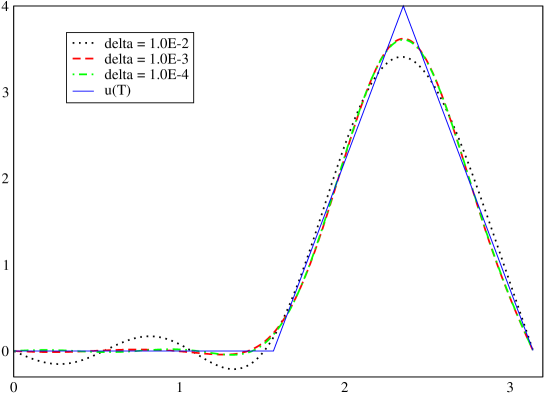
Figure 1: Exact and computed solutions at $t=T$ with various $\delta$’s and $s=3.8$.

	$L^{2}$-errors with $\delta=10^{-4}$		$L^{2}$-errors with $\delta=10^{-3}$		$L^{2}$-errors with $\delta=10^{-2}$
$t$	Computed	Predicted	Computed	Predicted	Computed	Predicted
T/4	4.25E-05	1.61E-03	2.96E-04	9.59E-03	7.82E-03	5.86E-02
T/2	3.18E-04	1.29E-02	1.20E-03	4.59E-02	2.39E-02	1.71E-01
3T/4	4.65E-03	1.04E-01	6.85E-03	2.20E-01	7.38E-02	5.02E-01
T	1.48E-01	8.33E-01	1.50E-01	1.06E-00	2.72E-01	1.47E-00

Table 1: $L^{2}$ errors of our regulared solutions and those of prediced in the theory are shown for $\delta=10^{-4},10^{-3},10^{-2}$. Here $s=3.8$.

Table 2 and Figure 2 are for $s=3.9$. The $L^{2}$ errors of $u^{\Gamma,u_{j0}}$ are again smaller than the predicted bounds for all cases. With $s=3.9$, the $\|u^{\Gamma,u_{j0}}(T)-u^{\Gamma,u_{j0}}(s)\|$ values are $0.0568,0.0623$ and $0.2110$ for $\delta=10^{-4},10^{-3},10^{-2}$, respectively. We observe that they are less than $K\delta=0.084$ except for $\delta=10^{-2}$. As in the previous case with $s=3.8$, for $\delta=10^{-2}$, we tried to generate a solution in the class by introducing different random noises, but it failed. It also should be noted that the $L^{2}$ errors are also smaller than the expected bounds, which implies that the quality of the solutions shown in Figure 2 are acceptable for all cases including when $\delta=10^{-2}$.

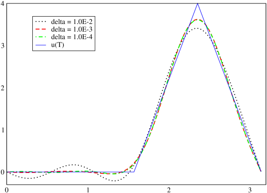
Figure 2: Exact and computed solutions at $t=T$ with various $\delta$’s and $s=3.9$.

	$L^{2}(\Omega)$ errors with $\delta=10^{-4}$		$L^{2}(\Omega)$ errors with $\delta=10^{-3}$		$L^{2}(\Omega)$ errors with $\delta=10^{-2}$
$t$	Computed	Predicted	Computed	Predicted	Computed	Predicted
T/4	4.25E-05	1.63E-03	2.96E-04	9.78E-03	7.83E-03	6.00E-02
T/2	3.18E-04	1.33E-02	1.20E-03	4.79E-02	2.39E-02	1.80E-01
3T/4	4.65E-03	1.09E-01	6.84E-03	2.34E-01	7.40E-02	5.39E-01
T	1.48E-01	8.88E-01	1.50E-01	1.15E-00	2.72E-01	1.62E-00

Table 2: $L^{2}$ errors of our regulared solutions and those of prediced in the theory are shown for $\delta=10^{-4},10^{-3},10^{-2}$. Here $s=3.9$.

References

- [1] S. Agmon and L. Nirenberg. Lower bounds and uniqueness theorems for solutions of differential equations in Hilbert space. Comm. Pure Appl. Math., 20:207–229, 1967.
- [2] A. S. Carasso. Overcoming Hölder continuity in ill-posed continuation problems. SIAM J. Numer. Anal., 31(6):1535–1557, 1994.
- [3] A. S. Carasso. Error bounds in nonsmooth image deblurring. SIAM J. Math. Anal., 28(3):656–668, 1997.
- [4] A. S. Carasso. Linear and nonlinear image deblurring : a documented study. SIAM J. Numer. Anal., 36(6):1659–1689, 1999.
- [5] A. S. Carasso. Logarithmic convexity and the ”slow evolution” constraint in ill-posed initial value problems. SIAM J. Math. Anal., 30(3):479–496, 1999.
- [6] A. S. Carasso. Direct blind deconvolution. SIAM J. Appl. Math., 61(6):1980–2007, 2001.
- [7] A. S. Carasso, D. S. Bright, and A. E. Vladár. Apex method and real-time blind deconvolution of scanning electron microscope imagery. Optical Engineering, 41(10):2499–2514, 2002.
- [8] I. P. Gavrilyuk, , W. Hackbusch, and B. N. Khoromskij. H-matrix approximation for the operator exponential with applications. Numer. Math., 92:83–111, 2002.
- [9] I. P. Gavrilyuk and V. L. Makarov. Exponentially convergent parallel discretization method for the first order evolution equations. Comput. Methods Appl. Math., 1:333–355, 2001.
- [10] I. P. Gavrilyuk and V. L. Makarov. Exponentially convergent algorithms for the operator exponential with applications to inhomogeneous problems in Banach spaces. SIAM J. Numer. Anal., 43(5):2144–2171, 2005.
- [11] I. P. Gavrilyuk, V. L. Makarov, and V. Vasylyk. A new estimate of the sinc method for linear parabolic problems including the initial point. Comput. Methods Appl. Math., 4:1–27, 2004.
- [12] J. Hadamard. Lectures on the Cauchy problems in linear partial differential equations. Yale University Press, New Haven, 1923.
- [13] F. John. Continuous dependence on data for solutions with a prescribed bound. Comm. Pure Appl. Math., 13:551–585, 1960.
- [14] K. Kwon and D. Sheen. A parallel method for the numerical solution of integro-differential equation with positive memory. Comput. Methods Appl. Mech. Engrg., 192(41–42):4641–4658 2003.
- [15] J. Lee and D. Sheen. An accurate numerical inversion of Laplace transforms based on the location of their poles. Comput & Math. Applic., 48(10–11):1415–1423, 2004
- [16] J. Lee and D. Sheen. A parallel method for backward parabolic problems based on the Laplace transformation. SIAM J. Numer. Anal., 44:1466–1486, 2006.
- [17] J. Lee and D. Sheen. The Laplace transformation method for backward parabolic problems with application to image deblurring. 2008. in preparation.
- [18] F. Lin. Remarks on a backward parabolic problem. Methods Appl. Anal., 10(2):245–252, 2003.
- [19] J. M. Marbán and C. Palencia. A new numerical method for backward parabolic problems in the maximum-norm setting. SIAM J. Numer. Anal, 40(4):1405–1420, 2002.
- [20] J. M. Marbán and C. Palencia. On the numerical recovery of a holomorphic mapping from a finite set of approximate values. Numer. Math., 91:57–75, 2002.
- [21] W. McLean, I. H. Sloan, and V. Thomée. Time discretization via Laplace transformation of an integro-differential equation of parabolic type. Numer. Math., 102:497–522, 2006.
- [22] W. McLean and V. Thomée. Time discretization of an evolution equation with Laplace transforms. IMA J. Numer. Anal., 24:439–463, 2004.
- [23] L. E. Payne. Improperly posed Problems in Partial Differential Equations. SIAM, Philadelphia, PA, 1975.
- [24] D. Sheen, I. H. Sloan, and V. Thomée. A parallel method for time-discretization of parabolic problems based on contour integral representation and quadrature. Math. Comp., 69(229):177–195, 2000.
- [25] D. Sheen, I. H. Sloan, and V. Thomée. A parallel method for time-discretization of parabolic equations based on Laplace transformation and quadrature. IMA J. Numer. Anal., 23(2):269–299, 2003.
- [26] V. Thomée. A high order parallel method for time discretization of parabolic type equations based on Laplace transformation and quadrature. Int. J. Numer. Anal. Model., 2:121–139, 2005.
- [27] L. N. Trefethen, J. A. C. Weideman, and T. Schmelzer. Talbot quadratures and rational approximations. BIT, 46(3):653–670, 2006.
- [28] J. A. C. Weideman. Optimizing Talbot’s contours for the inversion of the Laplace transform. SIAM J. Numer. Anal., 44(6):2342–2362 (electronic), 2006.
- [29] J. A. C. Weideman and L. N. Trefethen. Parabolic and hyperbolic contours for computing the Bromwich integral. Math. Comp., 76(259):1341–1356 (electronic), 2007.