Laplace transformation method for the Black-Scholes equation

Abstract.

In this paper we apply the innovative Laplace transformation method introduced by Sheen, Sloan, and Thomée (IMA J. Numer. Anal., 2003) to solve the Black-Scholes equation. The algorithm is of arbitrary high convergence rate and naturally parallelizable. It is shown that the method is very efficient for calculating various option prices. Existence and uniqueness properties of the Laplace transformed Black-Scholes equation are analyzed. Also a transparent boundary condition associated with the Laplace transformation method is proposed. Several numerical results for various options under various situations confirm the efficiency, convergence and parallelization property of the proposed scheme.

1. Introduction

As stock markets have become more sophisticated, so have their products. The simple buy/sell trades of the early markets have been replaced by more complex financial options and derivatives. These contracts can give investors various opportunities to tailor their dealings to their investment needs.

One of the main concerns about financial options is what the exact values of options are. For the simplest model in the case of constant coefficients, an exact pricing formula was derived by Black and Scholes, known as the Black-Scholes formula. However, in the general case of time and space dependent coefficients the exact pricing formula are not yet established, and thus numerical solutions have been used.

In order to describe an option price, let $x,K,t$ and $T$ denote the underlying asset price, the strike price, the time to maturity, and the expiry date of an option, respectively. As usual, $\sigma$ and $r$ represent the volatility of the underlying asset and the risk-free interest rate of the market, respectively. In this paper, we assume that $\sigma$ and $r$ depend on $x$ only. Then a European option price $u(x,t)$ satisfies the Black-Scholes equation:

$$\frac{\partial u}{\partial t}-\frac{1}{2}{\sigma^{2}x^{2}}\frac{\partial^{2}u}{\partial x^{2}}-rx\frac{\partial u}{\partial x}+ru=0,\quad(x,t)\in(0,\infty)\times(0,T],$$ (1.1)

where an initial condition $u_{0}(x)=u(x,0)$ is given by the initial contract of an option. The basket option based on $n$ assets $\mathbf{x}=(x_{1},\dots,x_{n})$ satisfies

$$\frac{\partial u}{\partial t}-\frac{1}{2}\sum^{n}_{i,j=1}a_{ij}x_{i}x_{j}\frac{\partial^{2}u}{\partial x_{i}\partial x_{j}}-\sum^{n}_{i=1}rx_{i}\frac{\partial u}{\partial x_{i}}+ru=0,$$ (1.2)

$$\qquad\qquad\qquad(\mathbf{x},t)\in(0,\infty)^{n}\times(0,T],$$

where $a_{ij}=\sum^{n}_{k=1}\sigma_{ik}\sigma_{jk}$, with $\sigma_{ij}$ representing the corelation between the assets $x_{i}$ and $x_{j}$.

Several numerical methods have been used for solving the Black-Scholes equation, for example in [32, 28] and [10] and the references therein, one can find popular numerical schemes for option pricing. Usually the time marching methods such as forward Euler, backward Euler and Crank-Nicolson schemes are used with a suitable spatial discretization scheme. In spite of the popularity of these time marching methods, a critical drawback of these schemes is that they usually require as many time steps as spatial meshes to balance the errors arising from discretization. In particular, for the estimation of basket options of reasonable size, the usual time marching schemes seem to be too slow in practice since the cost of solving an elliptic system to advance to a next time step is usually expensive. It is thus highly desirable to solve as small a number of elliptic solution steps as possible as well as to apply a very fast elliptic solver.

In this paper, we will focus on minimizing the number of elliptic solution steps by proposing the Laplace transformation method for the Black-Scholes equation, which is also naturally parallelizable. It will be shown that our method can dramatically reduce the computing time compared to the time marching schemes. Suitable contours should be chosen in order to have very fast convergence, and for this, we will estimate the resolvent of the Black-Scholes equation. Also, an exact transparent boundary condition will be given at which the infinite spatial domain is truncated.

There have been some related works in which the Laplace transformation method has been used, for instance in [7, 18, 25]. However, in these earlier papers the Laplace transformation method has been used to obtain the analytic solution of various options rather than to develop an efficient numerical scheme. In particular, in [18] the partial Laplace transformation is applied for American option pricing, and in [6, 24] the Mellin transformation which is similar to the Laplace transformation is used to evaluate the analytic solution of an option. Related with Laplace transformation methods there are other approaches based on the so-called $\mathcal{H}$-matrix approach; for instance, see [8, 9], and so on. Also, high-dimensional parabolic problems can be solved using sparse grids [11, 15, 16, 27]. Application of our Laplace transformation method using sparse grids to option pricing will also be interesting. Other approaches in the fast time-stepping methods can be found in [34, 20, 19].

In the following section, we will briefly describe the Laplace transformation method proposed by Sheen, Sloan, and Thomée in [30] with its numerical procedure and convergence. Then in §3 we will examine the properties of the Laplace transformed Black-Scholes equation including the solvability of the transformed equation, transparent boundary condition and the resolvent. Finally in §4 we will present several numerical results for various options and various situations with the parallelization property of the proposed scheme.

2. The Laplace transformation and its inversion

We begin with the abstract setting of a parabolic type equation so that the proposed scheme can be applicable to various problems. Consider

$$\frac{\partial u}{\partial t}+Au=f,\quad t\in(0.T];\quad u(0)=u_{0},$$ (2.1)

where $u_{0}$ is a given initial function and $A$ a spatial elliptic operator with its eigenvalues being located in the right half plane. (We added the source term $f(x,t)$, which is not present in (1.1) or in (1.2), in order to describe our method in more general setting.) For each $z$ in the complex plane, recall that the standard Laplace transform in time of a function $u(\cdot,t)$ is given by

$$\widehat{u}(\cdot,z):=\mathcal{L}[u](z)=\int_{0}^{\infty}u(\cdot,t)e^{-zt}\,dt.$$

Then the Laplace transformation of (2.1) is thus given in the form

$$z\widehat{u}+A\widehat{u} = u_{0}+\widehat{f}(\cdot,z),\quad z\in\Gamma,$$ (2.2)

from which the solution $\widehat{u}(z)=\widehat{u}(\cdot,z)$ is formally given by

$$\widehat{u}(\cdot,z)=(zI+A)^{-1}(u_{0}(\cdot)+\widehat{f}(\cdot,z)),$$ (2.3)

for each $z.$ We suppose that the real parts of singular points of $\widehat{f}(z)$ are less than some positive number.

The Laplace inversion formula ([2]) is given by

$$u(\cdot,t)=\frac{1}{2\pi\textrm{i}}\int_{\Gamma}\widehat{u}(\cdot,z)e^{zt}\,dz,$$ (2.4)

where the integral contour $\Gamma$ is a straight line parallel to the imaginary axis expressed as

$$\qquad\Gamma:=\{z\in\mathbb{C}:z(\omega)=\alpha+\textrm{i}\omega\,\textrm{where}\,\,\omega\in\mathbb{R}\,\,\textrm{increases from}\,-\infty\,\textrm{to}\,+\infty\}.$$ (2.5)

The constant $\alpha\in\mathbb{R}$ in the contour is called the Laplace convergence abscissa, and the value of $\alpha$ is required to be greater than the real part of any singularity of $\widehat{u}(z)$.

Inserting the explicit form of $z\in\Gamma$ given by (2.5) into Equation (2.4), one has

$$u(x,t)=\frac{e^{\alpha t}}{\pi}\int_{0}^{\infty}\big{[}\textrm{Re}\{\widehat{u}(x,\alpha+\textrm{i}\omega)\}\cos(\omega t)-\textrm{Im}\{\widehat{u}(x,\alpha+\textrm{i}\omega)\}\sin(\omega t)\big{]}\,d\omega.$$ (2.6)

Denoting by $\sum^{\prime}$ the summation with its first and the last summands being halved, an application of the composite trapezoidal rule to this integral leads to the direct method

$$u(x,t)\approx\frac{e^{\alpha t}}{T}{{\sum}^{\prime}}_{k=1}^{N-1}\left[\textrm{Re}\{\widehat{u}(x,\alpha+\frac{k\pi\textrm{i}}{T})\}\cos(\frac{k\pi t}{T})-\textrm{Im}\{\widehat{u}(x,\alpha+\frac{k\pi\textrm{i}}{T})\}\sin(\frac{k\pi t}{T})\right],$$

for some sufficiently large $N$ with the length of two mesh points $\pi/T$. Although this scheme can be easily implemented, its convergence rate is slow due to the truncation and discretization errors. In order to approximate the integration (2.6) fast and accurately, there have been numerous modifications, such as [3, 5, 8, 9, 23, 17, 29, 30, 13, 14, 22, 21, 31, 33, 35, 36, 38] and the references therein. In this paper, we will use the deformation of the contour introduced in [30], which gives an arbitrary high-order convergence rate with a hyperbolic type deformation.

2.1. Deformation of contour

For a concrete mathematical analysis, we assume that the spectrum $\sigma(A)$ of $A$ lies in a sector $\Sigma_{\delta}$ such that

$$\sigma(A)\subset\Sigma_{\delta}=\{z\in\mathbb{C}:|\arg z|\leq\delta,\,z\neq 0,\,\delta\in(0,\frac{\pi}{2})\},$$

and the resolvent $(zI+A)^{-1}$ of $A$ satisfies

$$\|(zI+A)^{-1}\|\leq\frac{M}{1+|z|},\quad\textrm{for }z\in\Sigma_{\delta}\cup B,$$

where $B$ is a small circle at the origin.

The first restriction is required to avoid the singular points of the integrand in (2.4). Since the problem (2.1) has a solution of the form

$$u(t)\left(=u(\cdot,t)\right)=\frac{1}{2\pi\textrm{i}}\int_{\Gamma}\big{(}zI+A\big{)}^{-1}\big{(}u_{0}+\widehat{f}(z)\big{)}e^{zt}\,dz,$$ (2.7)

the integral contour has to be kept away from the spectrum of $-A$ and the singular points of $\widehat{f}(z),$ when we deform the contour. In particular, since all eigenvalues of $-A$ and the singularities of $\widehat{f}(z)$ have real parts bounded by a positive number, this restriction is natural.

Observe that if $z\in\Gamma$ has negative real parts as $|z|$ becomes large, the discretization error in numerically evaluating the integrand in (2.7) will be reduced for positive $t$; thus it will be desirable to deform the contour to the left half plane as long as all the singularities are to the left of it. Based on this, Sheen et al. [30] proposed the smooth contour of hyperbola type as follows:

$$\Gamma=\{z\in\mathbb{C}:z(\omega)=\zeta(\omega)+\textrm{i}s\omega,\quad\omega\in\mathbb{R},\quad\omega\,\,\textrm{increasing}\},$$

where $\zeta(\omega)=\gamma-\sqrt{\omega^{2}+\nu^{2}}$. In this case, since the contour cuts the real line at $\gamma-\nu$, $\gamma$ and $\nu$ must be selected such that $\gamma-\nu$ is larger than the negative of the smallest eigenvalue of $A$ and the real parts of singularities of $\widehat{f}(z).$ Also $s$ should be chosen such that all the singularities of $\widehat{u}(\cdot,z)$ be to the left of the contour $\Gamma.$

Using the above deformed contour, the inversion formula can be written as an infinite integral with respect to a real variable,

$$u(\cdot,t)=\frac{1}{2\pi\textrm{i}}\int^{\infty}_{-\infty}\widehat{u}(\cdot,\zeta(\omega)+\textrm{i}s\omega)(\zeta^{\prime}(\omega)+\textrm{i}s)e^{(\zeta(\omega)+\textrm{i}s\omega)t}\textrm{d}\omega.$$

The infinite range of the above integration can be changed into to a finite region by the change of variables of the form

$$y(\omega)=\tanh\big{(}\frac{\tau\omega}{2}\big{)}\,\,\textrm{ and }\,\,\omega(y)=\frac{2}{\tau}\tanh^{-1}(y)=\frac{1}{\tau}\log\frac{1+y}{1-y},$$

for some $\tau>0$ and $y\in(-1,1)$. The above change of variables reduces from an integral on an infinite interval to one on a finite interval as follows:

$$u(\cdot,t)=\frac{1}{2\pi\textrm{i}}\int^{1}_{-1}\widehat{u}(\cdot,\zeta(\omega(y))+\textrm{i}s\omega(y))(\zeta^{\prime}(\omega(y))+\textrm{i}s)e^{(\zeta(\omega(y))+\textrm{i}s\omega(y))t}\omega^{\prime}(y)\textrm{d}y.$$ (2.8)

2.2. Semi-discrete approximation

The last integral formula (2.8) in the previous section can be discretized in time using a quadrature rule. Explicitly the semi-discrete approximation of $u(\cdot,t)$ is given by

$$U_{N,\tau}(\cdot,t)=\frac{1}{2\pi\textrm{i}}\frac{1}{N}\sum^{N-1}_{j=-N+1}\widehat{u}(\cdot,z_{j})\frac{\textrm{d}z}{\textrm{d}\omega}(\omega_{j})\frac{\textrm{d}\omega}{\textrm{d}y}(y_{j})e^{z_{j}t},$$ (2.9)

where

$$z_{j}=z(\omega_{j}),\quad\omega_{j}=\omega(y_{j})\quad\textrm{and}\quad y_{j}=\frac{j}{N},\quad\textrm{for}\,-N<j<N.$$

It is proved in [30] that the quadrature scheme (2.9) is of arbitrary high-order spectral convergence rate if in particular the source term $f$ has high-order regularity, stated as follows:

Theorem 2.1 (Sheen-Sloan-Thomée)

Let $u(t)$ be the solution of (2.1) and let $U_{N,\tau}(t)$ be its approximation defined by (2.9). Assume that $\widehat{f}(z)$ is analytic to the right of the contour $\Gamma$ and continuous onto $\Gamma$, with $\widehat{f}^{(j)}(z)$ bounded on $\Gamma$ for $j\leq r$ and $r$ an integer $\geq 1$, Then, for $t>r\tau$

$$\|U_{N,\tau}(t)-u(t)\|\leq\frac{C_{r,s}}{N^{r}}\Big{(}1+t^{r}+\frac{1}{\tau^{r}}\Big{)}e^{\gamma t}\Big{(}1+\log_{+}\frac{1}{t-r\tau}\Big{)}(\|u_{0}\|+\max_{k\leq r}\sup_{z\in\Gamma}\|\widehat{f}^{(k)}(z)\|).$$ (2.10)

Three important remarks should be stressed.

Remark 2.2.

The implication of the above theorem without source term $f$ as in our option pricing is that the scheme is of order $O(\frac{1}{N^{r}})$ with an arbitrarily large $r>0$ since $\widehat{f}\equiv 0$ is certainly analytic and $\widehat{f}^{(r)}(z)$ is bounded on $\Gamma$ for positive integer $r.$ This implies that the discretization errors in the time direction using the Laplace transformation method will be negligible compared to those caused from the spatial discretization part in solving the Black-Scholes equation.

Remark 2.3.

In the summand (2.9), an important observation is that

$$\widehat{u}(\cdot,z_{j})\frac{\textrm{d}z}{\textrm{d}\omega}(\omega_{j})\frac{\textrm{d}\omega}{\textrm{d}y}(y_{j}),\,\,j=0,\cdots,N,$$

are independent of $t$. Therefore, we only have to approximate $\widehat{u}(\cdot,z_{j})$ only once by solving the complex-valued elliptic problem (2.2) for a set of $z_{j},j=0,1,\cdots,N.$ Then, if we need the option pricing at a different time $t$, the same set of spatial solutions $\widehat{u}(\cdot,z_{j}),j=0,1,\cdots,N$, can be used in the evaluation of the summation (2.9) with the only change in $e^{z_{j}t},$ for the needed time $t.$

Remark 2.4.

Notice that each elliptic problem (2.2) for a $z_{j}$ from the set of $z_{j},j=0,1,\cdots,N,$ is independent of other elliptic problems for the remaining $z_{j}$’s. This will minimize communication times in solving the elliptic problems (2.2) in parallel by assigning each processor to solve an independent elliptic problem without communicating with other processors during solving its assigned problem.

3. Laplace transformation method for the Black-Scholes equation

In this section, we will apply the Laplace transformation method to the Black-Scholes equation depending on one stock asset. A basket option depending on several assets can be extended from the following numerical scheme and analyzed in a similar way. Taking Laplace transforms of (1.1), we have

$$z\widehat{u}-\frac{1}{2}\sigma^{2}x^{2}\frac{\partial^{2}\widehat{u}}{\partial x^{2}}-rx\frac{\partial\widehat{u}}{\partial x}+r\widehat{u}=u_{0},\quad(x,z)\in\mathbb{R}_{+}\times\Gamma.$$ (3.1)

In what follows, we will examine the solvability of the above equation and the resolvent of the Black-Scholes equation.

3.1. The weak formulation of the Laplace transformed equation

For a concrete mathematical analysis, we restrict our attention to a European put option. Since the boundary condition of a put option vanishes at infinity, the partial differential equation can be reformulated as a weak problem in a weighted Sobolev space. Let $L^{2}(\mathbb{R}_{+})$ be the space of square integrable complex-valued functions on $\mathbb{R}_{+}$ which is endowed with the inner-product $(v,w)=$ $\int_{\mathbb{R}_{+}}v(x)\overline{w}(x)\,dx$ and the norm $\|v\|_{L^{2}(\mathbb{R}_{+})}=\sqrt{(v,v)}.$ Then following [1], the weighted Sobolev spaces are defined:

Definition 3.1.

Let $\mathcal{V}$ be the weighted Sobolev space defined by

$$\mathcal{V}=\{v\in L^{2}(\mathbb{R}_{+}):\,x\frac{\partial v}{\partial x}\in L^{2}(\mathbb{R}_{+})\},$$

equipped with the the semi-norm and the norm

$$|v|_{\mathcal{V}}=\Big{(}\int_{0}^{\infty}\left|x\frac{\partial v}{\partial x}\right|^{2}\,dx\Big{)}^{\frac{1}{2}},\quad\|v\|_{\mathcal{V}}=\Big{(}\int_{0}^{\infty}|v|^{2}+\left|x\frac{\partial v}{\partial x}\right|^{2}\,dx\Big{)}^{\frac{1}{2}}.$$

Similarly, let $\mathcal{Z}$ be the weighted Sobolev space defined by

$$\mathcal{Z}=\{v\in L^{\infty}(\mathbb{R}_{+}):x\frac{\partial v}{\partial x}\in L^{\infty}(\mathbb{R}_{+})\},$$

equipped with the the semi-norm and the norm

$$|v|_{\mathcal{Z}}=\operatorname{ess.\,sup}_{x\in\mathbb{R}_{+}}\left|x\frac{\partial v}{\partial x}\right|,\quad\|v\|_{\mathcal{Z}}=\max\left\{\operatorname{ess.\,sup}_{x\in\mathbb{R}_{+}}\left|v\right|,\,\operatorname{ess.\,sup}_{x\in\mathbb{R}_{+}}\left|x\frac{\partial v}{\partial x}\right|\right\}.$$

Since the boundary value vanishes at infinity, we have the following Poincaré-type inequality, which is an extension of the real-valued version, Lemma 2.7 given in [1]:

Lemma 3.2

The following bound holds:

$$\|v\|_{L^{2}(\mathbb{R}_{+})}\leq 2|v|_{\mathcal{V}}\qquad\forall v\in\mathcal{V}.$$ (3.2)

Proof.

Let $v\in\mathcal{V}$ be arbitrary. Then, by integration by parts, the following relation holds:

$$-\int_{\mathbb{R}_{+}}v\overline{v}\,dx=\int_{\mathbb{R}_{+}}xv\overline{v}_{x}\,dx+\int_{\mathbb{R}_{+}}x\overline{v}v_{x}\,dx.$$

Thus we obtain

$$\int_{\mathbb{R}_{+}}|v|^{2}\,dx\leq 2\Big{(}\int_{\mathbb{R}_{+}}|v|^{2}\,dx\Big{)}^{\frac{1}{2}}\Big{(}\int_{\mathbb{R}_{+}}|xv_{x}|^{2}\,dx\Big{)}^{\frac{1}{2}}.$$

This completes the proof. ∎

From now on, assume that the initial data $u_{0}\in\mathcal{V}^{\prime}$, where $\mathcal{V}^{\prime}$ is the dual space of $\mathcal{V}$. Denote by $\mathcal{V}^{\prime}$ the topological dual space of $\mathcal{V}$ with the norm defined by

$$\|u\|_{\mathcal{V}^{\prime}}=\sup_{v\in\mathcal{V}\setminus\{0\}}\frac{\left\langle u,v\right\rangle}{\|v\|_{\mathcal{V}}},$$

where $\left\langle\cdot,\cdot\right\rangle$ is the duality pairing of $\mathcal{V}^{\prime}$ and $\mathcal{V}$.

Then, multiplying (3.1) by a test function $v\in\mathcal{V}$ and integrating on $\mathbb{R}_{+}$, one obtains the weak problem of (3.1) as follows: For each $z\in\Gamma$, find $\widehat{u}(z)\in\mathcal{V}$ such that

$$A_{z}(\widehat{u},v)=\left\langle u_{0},v\right\rangle\quad\forall v\in\mathcal{V},$$ (3.3)

where the bilinear form $A_{z}(\cdot,\cdot):\mathcal{V}\times\mathcal{V}\rightarrow\mathbb{C}$ is defined by

$$A_{z}(u,v)=z(u,v)+B(u,v)\quad\forall u,v\in\mathcal{V}.$$ (3.4)

where

$$B(u,v)=\frac{1}{2}\int_{\mathbb{R}_{+}}\sigma^{2}(x)x^{2}\frac{\partial u}{\partial x}\frac{\partial\overline{v}}{\partial x}\,dx + \int_{\mathbb{R}_{+}}\Big{(}-r(x)+\sigma^{2}(x)+x\sigma(x)\frac{\partial\sigma}{\partial x}\Big{)}x\frac{\partial u}{\partial x}\overline{v}\,dx$$

$$+\int_{\mathbb{R}_{+}}r(x)u\overline{v}\,dx,$$

The bilinear form $A_{z}(\cdot,\cdot)$, of course, depends on $z\in\Gamma,$ and so does the solution $\widehat{u}.$

Assumption 3.3

Assume that $\sigma\in\mathcal{Z}$ and $r\in L^{\infty}(\mathbb{R}_{+}).$ Moreover, assume that there exists a positive constant $\underline{\sigma}$ such that for all $x\in\mathbb{R}_{+}$ such that

$$0<\underline{\sigma}\leq\sigma(x).$$

Set

$$\mu=\begin{cases}(\|r\|_{L^{\infty}(\mathbb{R}_{+})}-\sigma^{2})^{2}/(\underline{\sigma})^{2},&\text{ if }\sigma(x)\text{ is a constant},\\ (\|r\|_{L^{\infty}(\mathbb{R}_{+})}+2\|\sigma\|_{\mathcal{Z}}^{2})^{2}/(\underline{\sigma})^{2},&\text{ otherwise.}\end{cases}$$

We now have the following two lemmas for the continuity and coercivity of $A_{z}(\cdot,\cdot):\mathcal{V}\times\mathcal{V}\rightarrow\mathbb{C}$.

Lemma 3.4

Under Assumption 3.3, the bilinear form $A_{z}(\cdot,\cdot):\mathcal{V}\times\mathcal{V}\rightarrow\mathbb{C}$ is continuous.

Proof.

Let $u,v\in\mathcal{V}.$ Then,

$$\Big{|}\int_{\mathbb{R}_{+}}\frac{1}{2}\sigma^{2}(x)x^{2}\frac{\partial u}{\partial x}\frac{\partial\overline{v}}{\partial x}\,dx\Big{|} \leq\frac{1}{2}|\sigma|_{\mathcal{Z}}^{2}|u|_{\mathcal{V}}|v|_{\mathcal{V}},$$

$$\Big{|}\int_{\mathbb{R}_{+}}\Big{(}-r(x)+\sigma^{2}(x)+x\sigma(x)\frac{\partial\sigma}{\partial x}\Big{)}x\frac{\partial u}{\partial x}\overline{v}\,dx\Big{|} \leq\underline{\sigma}\sqrt{\mu}\,|u|_{\mathcal{V}}\|v\|_{L^{2}(\mathbb{R}_{+})}$$

$$\leq 2\underline{\sigma}\sqrt{\mu}\,|u|_{\mathcal{V}}|v|_{\mathcal{V}},$$

$$\Big{|}\int_{\mathbb{R}_{+}}\Big{(}z+r(x)\Big{)}u\overline{v}\,dx\Big{|} \leq(|z|+\|r\|_{L^{\infty}(\mathbb{R}_{+})})|u|_{\mathcal{V}}|v|_{\mathcal{V}},$$

where Lemma 3.2 is applied in the bound of the second inequality. Therefore the bilinear form $A_{z}(\cdot,\cdot):\mathcal{V}\times\mathcal{V}\rightarrow\mathbb{C}$ is continuous. ∎

Lemma 3.5

Under Assumption 3.3, there is a non-negative constant $C_{1}$, which is independent of $u$ and $z$, such that for all $u\in\mathcal{V}$

$$\operatorname{Re}\{A_{z}(u,u)\}\geq\frac{\underline{\sigma}^{2}}{4}|u|^{2}_{\mathcal{V}}-(|z|+C_{1})\|u\|^{2}_{L^{2}(\mathbb{R}_{+})}.$$

Proof.

Under Assumption 3.3, the following result is known in [1],

$$\operatorname{Re}\{B(u,u)\}\geq\frac{\underline{\sigma}^{2}}{4}|u|^{2}_{\mathcal{V}}-\mu\|u\|^{2}_{L^{2}(\mathbb{R}_{+})}.$$ (3.5)

Let $u\in\mathcal{V}$ be arbitrary. Then,

$$\int_{\mathbb{R}_{+}}\frac{1}{2}\sigma^{2}(x)x^{2}\frac{\partial u}{\partial x}\frac{\partial\overline{u}}{\partial x}\,dx \geq\frac{\underline{\sigma}^{2}}{2}|u|_{\mathcal{V}}^{2},$$

$$\Big{|}\operatorname{Re}\{\int_{\mathbb{R}_{+}}\Big{(}-r(x)+\sigma^{2}(x)+x\sigma(x)\frac{\partial\sigma}{\partial x}\Big{)}x\frac{\partial u}{\partial x}\overline{u}\,dx\}\Big{|} \leq\underline{\sigma}\sqrt{\mu}\,|u|_{\mathcal{V}}\|u\|_{L^{2}(\mathbb{R}_{+})}$$

$$\leq\frac{\underline{\sigma}^{2}}{4}|u|^{2}_{\mathcal{V}}+\mu\|u\|^{2}_{L^{2}(\mathbb{R}_{+})},$$

$$\Big{|}\operatorname{Re}\{\int_{\mathbb{R}_{+}}\Big{(}z+r(x)\Big{)}u\overline{u}\,dx\}\Big{|} \leq(|z|+\|r\|_{L^{\infty}(\mathbb{R}_{+})})\|u\|^{2}_{L^{2}(\mathbb{R}_{+})},$$

where Young’s inequality is used in the bound of the second inequality and $\mu$ depends on $\underline{\sigma}$. A combination of these inequalities completes the lemma. ∎

The compactness of embedding $L^{2}(\mathbb{R}_{+})\hookrightarrow\mathcal{V}$, Lemma 3.4 and Lemma 3.5 imply that there is a unique solution in the case of European put options. We summarize the above results in the following theorem.

Theorem 3.6

Suppose $u_{0}\in\mathcal{V}^{\prime}$. Then, under Assumption 3.3 Problem (3.3) has a unique solution $\widehat{u}\in\mathcal{V}.$

3.2. Resolvent of the Black-Scholes equation

In §2, the resolvent of a spatial operator is assumed to be bounded in a given sector. This assumption for the Black-Scholes equation will be verified in this subsection.

Denote by $R(z,-B)=(zI+B)^{-1}$ the resolvent of $-B$, so that for each $f\in\mathcal{V}^{\prime}$, $v=R(z,-B)f$ is the solution of

$$B(v,\phi)+z(v,\phi)=\left\langle f,\phi\right\rangle,\qquad\forall\phi\in\mathcal{V}.$$ (3.6)

Then we have the following lemma, which is an extension of Lemma 2.1 in [4].

Lemma 3.7

Under Assumption 3.3, for any $\theta\in(\frac{1}{2}\pi,\pi)$ there are $C=C(\theta)\geq 0$ and $\kappa=\kappa(\theta,r,\sigma)>0$, independent of $z$ and $f$, such that

$$\|R(z,-B)f\|_{L^{2}({\mathbb{R}_{+}})}\leq\frac{C}{|z-\kappa|}\|f\|_{L^{2}({\mathbb{R}_{+}})},\qquad\text{for }z\in\Sigma_{\kappa,\theta},\,\,f\in L^{2}({\mathbb{R}_{+}})$$

where $\Sigma_{\kappa,\theta}=\{z\in\mathbb{C}:|\arg(z-\kappa)|\leq\theta\}$. Explicitly, the coefficients are given by $C=(1+\frac{1}{2}\delta)(1+\delta^{2})$ and $\kappa=\left(1+\frac{\delta^{2}}{2}\right)\mu,$ where $\delta=\tan\frac{\theta}{2}.$

Proof.

For $z\in\Sigma_{\kappa,\theta}$, we write

$$z-\kappa=(\xi+\textrm{i}\eta)^{2}=\xi^{2}-\eta^{2}+2\textrm{i}\xi\eta\qquad\text{with}\,\,\xi+\textrm{i}\eta\in\Sigma_{0,\theta/2},\,\,\xi,\eta\in\mathbb{R},$$

for any $\kappa>0.$ Setting $\delta=\tan\frac{\theta}{2}$, we see that $\delta>1$ and $|\eta|\leq\delta\xi.$ and thus the following inequality holds:

$$\xi^{2}\leq|z-\kappa|=\xi^{2}+\eta^{2}\leq(1+\delta^{2})\xi^{2}.$$

Set

$$F=B(v,v)+z\|v\|_{L^{2}(\mathbb{R}_{+})}^{2}.$$

Taking the real part of $F$, we obtain

$$\operatorname{Re}B(v,v)+(\kappa+\xi^{2}-\eta^{2})\|v\|_{L^{2}(\mathbb{R}_{+})}^{2}=\operatorname{Re}F.$$

By the inequality (3.5) we have

$$\frac{\underline{\sigma}^{2}}{4}|v|_{\mathcal{V}}^{2}+(\kappa+\xi^{2}-\eta^{2}-\mu)\|v\|_{L^{2}(\mathbb{R}_{+})}^{2}\leq|F|.$$ (3.7)

By taking the imaginary part of $F$, we have

$$\operatorname{Im}B(v,v)+2\xi\eta\|v\|_{L^{2}(\mathbb{R}_{+})}^{2}=\operatorname{Im}F,$$

and since $\operatorname{Im}B(v,v)=\operatorname{Im}\int_{\mathbb{R}_{+}}\Big{(}-r(x)+\sigma^{2}(x)+x\sigma(x)\frac{\partial\sigma}{\partial x}\Big{)}x\frac{\partial v}{\partial x}\overline{v}\,dx$,

$$2\xi|\eta|\,\|v\|_{L^{2}(\mathbb{R}_{+})}^{2}\leq|F|+\underline{\sigma}\sqrt{\mu}\,|v|_{\mathcal{V}}\|v\|_{L^{2}(\mathbb{R}_{+})}.$$

Multiplying by $\frac{1}{2}\delta=\frac{1}{2}\tan(\frac{1}{2}\theta)$ the last estimate, we have

$$\eta^{2}\|v\|_{L^{2}(\mathbb{R}_{+})}^{2}\leq\delta|\eta|\,\|v\|_{L^{2}(\mathbb{R}_{+})}^{2}\leq\frac{1}{2}\delta|F|+\frac{1}{2}\delta\,\underline{\sigma}\sqrt{\mu}\,|v|_{\mathcal{V}}\|v\|_{L^{2}(\mathbb{R}_{+})}.$$

Adding this to (3.7), we obtain

$$\frac{\underline{\sigma}^{2}}{4}|v|_{\mathcal{V}}^{2}+(\kappa+\xi^{2}-\mu)\|v\|_{L^{2}(\mathbb{R}_{+})}^{2}\leq(1+\frac{1}{2}\delta)|F|+\frac{\underline{\sigma}^{2}}{8}|v|_{\mathcal{V}}^{2}+\frac{\delta^{2}\mu}{2}\|v\|_{L^{2}(\mathbb{R}_{+})}^{2}.$$

With the choice of

$$\kappa=\mu+\frac{\delta^{2}\mu}{2}=\left(1+\frac{\delta^{2}}{2}\right)\mu,$$

we have the following inequality

$$\frac{\underline{\sigma}^{2}}{8}|v|_{\mathcal{V}}^{2}+\xi^{2}\|v\|_{L^{2}(\mathbb{R}_{+})}^{2}\leq(1+\frac{1}{2}\delta)|F|.$$

If $f\in L^{2}(\mathbb{R}_{+})$, we take $\phi=v$ in (3.6), then we have

$$\frac{\underline{\sigma}^{2}}{8}|v|_{\mathcal{V}}^{2}+\xi^{2}\|v\|_{L^{2}(\mathbb{R}_{+})}^{2}\leq(1+\frac{1}{2}\delta)\Big{|}\int_{\mathbb{R}_{+}}fv\,dx\Big{|}\leq(1+\frac{1}{2}\delta)\|f\|_{L^{2}(\mathbb{R}_{+})}\|v\|_{L^{2}(\mathbb{R}_{+})},$$

and therefore

$$\|R(z,-B)f\|_{L^{2}(\mathbb{R}_{+})}\leq\frac{1+\frac{1}{2}\delta}{\xi^{2}}\|f\|_{L^{2}(\mathbb{R}_{+})}\leq\frac{(1+\frac{1}{2}\delta)(1+\delta^{2})}{|z-\kappa|}\|f\|_{L^{2}(\mathbb{R}_{+})}.$$

This completes the proof. ∎

From this lemma one can determine the location of a integration contour. In particular, if one sets the asymptotic slope of a hyperbola as $s$, the contour has to cut the real line at a point which is larger than

$$\kappa=\left(1+\frac{\tan^{2}(\frac{1}{2}\arctan(s))}{2}\right)\,\mu.$$

In the special cast that $r(x)=r$ and $\sigma(x)=\sigma$ are constants, $\kappa$ can be given by

$$\kappa=\left(1+\frac{\tan^{2}(\frac{1}{2}\arctan(s))}{2}\right)\,\frac{|r-\sigma^{2}|^{2}}{\sigma^{2}}.$$ (3.8)

3.3. The transparent boundary condition

As one can see in (1.1) or (1.2), the space domain of the underlying asset of an option is an unbounded set. To apply a numerical scheme, one usually truncates the infinite domain into a finite one, and then imposes a suitable boundary condition on the boundary. Let $L$ be a sufficiently large asset price. One then has the following version of the Black-Scholes equation truncated at $x=L$.

$$\frac{\partial u}{\partial t}-\frac{1}{2}{\sigma^{2}x^{2}}\frac{\partial^{2}u}{\partial x^{2}}-rx\frac{\partial u}{\partial x}+ru = 0,\quad(x,t)\in(0,L)\times(0,T],$$ (3.9)

$$u(x,t) = g(x,t),\quad(x,t)\in\partial(0,L)\times(0,T],$$ (3.10)

$$u(x,0) = u_{0},\quad x\in[0,L].$$ (3.11)

In many cases, the boundary condition on the artificial boundary $x=L$ is imposed by extending a given payoff function. For example, European put options assume $u(L,t)=0$ and European call options assume $\frac{\partial u}{\partial x}(L,t)=1$. In [12], the errors caused by Dirichlet boundary conditions on the artificial boundary are estimated and thus one can determine a suitable truncation asset price for the artificial boundary to meet a given error tolerance.

Instead of such artificial boundary conditions, a transparent boundary condition is introduced in [1] with which one can evaluate the solution in the truncated domain without any truncation error. However, the boundary condition in [1] is an integro-differential one, which needs some suitable numerical schemes to approximate it that will produce other possibly significant errors. We will analyze the transparent boundary condition in more detail and then depart from such an integro-differential type, by implementing the boundary condition in the Laplace transformed setting instead of the usual space-time setting. Our transparent boundary condition is motivated by the following proposition.

Proposition 3.8

Assume that the coefficients $\sigma$ and $r$ in (3.1) are constants and that $L>0$ is sufficiently large so that $\operatorname{supp}(u_{0})\subset[0,L)$. Then among the solutions $\widehat{u}(x,z)$ satisfying (3.1) there is a component, $\widehat{u}_{+}$, satisfying the following:

$$\frac{\partial\widehat{u}_{+}}{\partial x}(x,z)=\frac{1}{x\sigma^{2}}\left\{-(r-\frac{1}{2}\sigma^{2})-\sqrt[+]{\big{(}r-\frac{1}{2}\sigma^{2}\big{)}^{2}+2\sigma^{2}(r+z)}\right\}\widehat{u}_{+}(x,z)$$ (3.12)

$\quad\forall x\in(L,\infty),$ where $\operatorname{Re}\{\sqrt[+]{z}\}>0$ for nonzero $z\in\mathbb{C}$.

Proof.

Take the change of variables, $y=\log x$, to (3.1). Denoting by $\widehat{v}$ its solution, owing to $\operatorname{supp}(u_{0})\in[0,L)$, one observes that $\widehat{v}$ satisfies the right exterior problem

$$z\widehat{v}-\frac{1}{2}\sigma^{2}\frac{\partial^{2}\widehat{v}}{\partial y^{2}}-(r-\frac{1}{2}\sigma^{2})\frac{\partial\widehat{v}}{\partial y}+r\widehat{v}=0,\quad(y,z)\in(L,\infty)\times\Gamma.$$ (3.13)

Among the two linearly independent solutions, we take the component which vanishes at infinity, which is given as follows:

$$\widehat{v}_{+}(y,z)=\exp\Big{(}\left\{\frac{-(r-\sigma^{2}/2)}{\sigma^{2}}-\frac{1}{\sigma^{2}}\sqrt[+]{\big{(}r-\frac{1}{2}\sigma^{2}\big{)}^{2}+2\sigma^{2}(r+z)}\right\}y\Big{)}.$$

Restoring the change of variable, $x=e^{y}$, and denoting by $\widehat{u}_{+}(x)=\widehat{v}_{+}(y)$, one gets

$$\widehat{u}_{+}(x,z)=x^{\left\{\frac{-(r-\sigma^{2}/2)}{\sigma^{2}}-\frac{1}{\sigma^{2}}\sqrt[+]{\big{(}r-\frac{1}{2}\sigma^{2}\big{)}^{2}+2\sigma^{2}(r+z)}\right\}}.$$

Thus, by differentiating with respect to $x$, one arrives at

$$\frac{\partial\widehat{u}_{+}}{\partial x}(x,z)=\frac{1}{x\sigma^{2}}\left\{-(r-\sigma^{2}/2)-\sqrt[+]{\big{(}r-\frac{1}{2}\sigma^{2}\big{)}^{2}+2\sigma^{2}(r+z)}\right\}\widehat{u}_{+}(x,z).$$

Thus, $\widehat{u}_{+}$ satisfies the equation (3.12), which completes the proof. ∎

Due to Proposition 3.8, by choosing $L>0$ sufficiently large so that $\operatorname{supp}(u_{0})\in[0,L),$ we propose the following transparent boundary condition at $x=L:$

$$\frac{\partial\widehat{u}}{\partial x}(L,z)=\frac{1}{L\sigma^{2}}\left\{-(r-\frac{1}{2}\sigma^{2})-\sqrt[+]{\big{(}r-\frac{1}{2}\sigma^{2}\big{)}^{2}+2\sigma^{2}(r+z)}\right\}\widehat{u}(L,z)\quad\forall z\in\Gamma.$$ (3.14)

Remark 3.9.

By the Laplace inversion of (3.14), the transparent boundary condition in the space-time domain is given by

$$\frac{\partial u}{\partial x}(L,t)=\frac{1}{L\sigma^{2}}\left\{-(r-\frac{\sigma^{2}}{2})u(L,t)-\frac{\sqrt{2}\sigma}{\sqrt{\pi}}e^{-\eta t}\frac{\partial}{\partial t}\int^{t}_{0}\frac{u(L,\tau)e^{\eta\tau}}{\sqrt{t-\tau}}d\tau\right\},$$ (3.15)

where $\eta=\frac{(r-\sigma^{2}/2)^{2}}{2\sigma^{2}}+r$. In the derivation of (3.15), the following equalities are used:

$$\mathcal{L}\left\{\frac{\partial}{\partial t}\int^{t}_{0}\frac{1}{\sqrt{t-\tau}}u(\tau)e^{\eta\tau}d\tau\right\} = z\mathcal{L}\left\{\int^{t}_{0}\frac{1}{\sqrt{t-\tau}}u(\tau)e^{\eta\tau}d\tau\right\}$$

$$= z\mathcal{L}\left\{\frac{1}{\sqrt{t}}\right\}\mathcal{L}\left\{u(t)e^{\eta t}\right\}$$

$$= \sqrt{\pi}\sqrt{z}\widehat{u}(z-\eta).$$

In solving the partial integro-differential equation (3.12) with (3.15) using a Crank-Nicolson type of time-marching algorithm, one usually needs an expensive algorithm in computing time and memory. We will compare our Laplace transformation method with the Crank-Nicolson method in §4, and conclude superiority in using our method.

4. Numerical results

We applied the Laplace transformation method for time discretization while the standard piecewise linear ($P_{1}$) finite element method for the space discretization is used. Using an analytic solution for the first two examples, we can compare the convergence rate of the proposed scheme. In Example 4.2 we examine the effects of the Dirichlet boundary condition and the transparent boundary condition (3.14) in the calculation of option prices.

In calculating the numerical values of the analytical solution, the error function $erf(x)$ is evaluated by using the algorithm on page 213 of Numerical Recipes in Fortran [26] which has 16-digit precision. The reduction rate and speedup are defined by

$$\textrm{reduction rate}=\log_{2}\frac{\|u_{\Delta x}-u_{\textrm{exact}}\|_{L^{2}(0,L)}}{\|u_{\frac{\Delta x}{2}}-u_{\textrm{exact}}\|_{L^{2}(0,L)}},$$

where $u_{\Delta x}$ denotes the numerical solution with the spatial mesh size $\Delta x$, and

$$\textrm{speed up}=\frac{\textrm{time consumption}}{\textrm{time consumption using 1-CPU}}.$$

Example 4.1 (European put option with constant coefficients)

We consider an European put option with coefficients $r=0.05$, $\sigma=0.3$, $T=1.0$ and $K=50$ and we truncate the domain at $L=200$.

For the numerical solutions, the boundary condition at $x=0$ in (3.10) is given by

$$u(x,t)=Ke^{-rt},\quad(x,t)\in\{0\}\times(0,T],$$

while that at $x=L$

$$u(x,t)=0,\quad(x,t)\in\{L\}\times(0,T].$$ (4.1)

Although an analytic solution to this example is given by Black and Scholes, it is our aim to compare convergence rates for the proposed scheme and the standard time-marching algorithms such as Crank-Nicolson scheme. Table 1 shows convergence rate for the Crank-Nicolson scheme. As can be expected, it gives first-order convergence rate. Table 2 shows that the choice of 15 $z$-points in the contour with the proposed method is enough to obtain the same level of tolerance attained using 640 time steps with the Crank-Nicolson method. Observe that for each $z$-point the cost of solving the complex-valued elliptic problem using the proposed method is almost comparable to that of advancing one step forward by solving the real-valued elliptic problem with the time-marching algorithms.

In the proposed scheme, we need the value of $\kappa$ as in Lemma 3.7 to determine the location of a integration contour. Since the coefficients are constants, if we choose the asymptotic slope of the contour as $0.4$, we have $\kappa=0.01811$ by (3.8), and therefore the contour has to cut the real line at a point greater than 0.01811. Under this constraint, we choose the optimal parameters which are suggested in [37], and these parameters are attached in Table 3 in the case that the evaluation time is 1.0 for different iteration numbers. In particular, Table 3 says that 12 iterations are enough to balance with the space discretization of 2560 spatial meshes.

Time steps	Number of space meshes	Mesh size	Error in $L^{2}$	Reduction rate
10	10	20	2.928
20	20	10	0.7536	1.958
40	40	5	0.1878	2.004
80	80	2.5	0.4695E-01	2.000
160	160	1.25	0.1174E-01	2.000
320	320	5/8	0.2934E-02	2.000
640	640	5/16	0.7337E-03	2.000

Table 1. Example 4.1 with the Crank-Nicolson method

Number of $z$	Number of space meshes	Mesh size	Error in $L^{2}$	Reduction rate
15	10	20	2.924
15	20	10	0.7524	1.959
15	40	5	0.1876	2.004
15	80	2.5	0.4688E-01	2.000
15	160	1.25	0.1172E-01	2.000
15	320	5/8	0.2930E-02	2.000
15	640	5/16	0.7327E-03	2.000

Table 2. Example 4.1 with the Laplace transformation method

Number of $z$	Number of space meshes	$L^{2}$-Error	Reduction rate	$\gamma$	$\nu$	$s$	$\tau$
3	2560	0.6397E-00		13.48	12.42	0.4213	0.16500
6	2560	0.1705E-01	5.229	26.95	24.84	0.4213	0.09385
9	2560	0.3434E-03	5.634	40.43	37.26	0.4213	0.06809
12	2560	0.5642E-04	2.605	53.90	49.68	0.4213	0.05430
15	2560	0.4731E-04	0.003	67.38	62.09	0.4213	0.04556
18	2560	0.4721E-04	0.001	80.86	74.51	0.4213	0.03947
21	2560	0.4717E-04	0.000	94.33	86.93	0.4213	0.03494

Table 3. Contour Parameters for Example 4.1

Example 4.2 (European put option with transparent boundary condition)

We consider a European put option with coefficients $r=0.05$, $\sigma=0.3$, $T=1.0$ and $K=50$ and we truncate the domain at $L=50$.

In this example, we truncate the domain at the strike price, and then we replace the Dirichlet boundary condition (4.1) with the transparent boundary condition given in (3.14). An identical contour as in the previous example has been adopted. Table 4 shows that the Dirichlet boundary condition with the domain truncation makes a significant error, which cannot be overcome by mesh refinement. Table 5, however, gives second order convergence which is shown in Table 2 although its domain is much smaller than that for Example 4.1. Indeed, comparing the same mesh sizes in Table 5 and Table 2, one can observe the numerical values are almost identical. In Figure 1 we can see the difference between the transparent boundary condition and the Dirichlet boundary.

Number of $z$	Number of space meshes	Mesh size	Error in $L^{2}$	Reduction rate
15	10	5	10.35
15	20	2.5	10.40	-0.007
15	40	1.25	10.41	-0.002
15	80	5/8	10.42	0.000
15	160	5/16	10.42	0.000
15	320	5/32	10.42	0.000
15	640	5/64	10.42	0.000

Table 4. Example 4.2 with the Dirichlet boundary condition at $L=50$

Number of $z$	Number of space meshes	Mesh size	Error in $L^{2}$	Reduction rate
15	10	5	0.1870
15	20	2.5	0.4656E-01	2.006
15	40	1.25	0.1163E-01	2.001
15	80	5/8	0.2907E-02	2.000
15	160	5/16	0.7267E-03	2.000
15	320	5/32	0.1817E-03	1.999
15	640	5/64	0.4551E-04	1.998

Table 5. Example 4.2 with the transparent boundary condition (3.14) at $L=50$

Figure 1. Comparison between the Dirichlet boundary condition and the transparent boundary condition (3.14) in Example 4.2

Example 4.3 (Basket option with two underlying assets)

We consider a European put basket option with two underlying assets having coefficients $r=0.05$, $a_{11}=0.09$, $a_{22}=0.09$, $a_{12}=a_{21}=-0.018$, time to maturity=1.0, artificial boundary $L_{1}=300,L_{2}=300$ and payoff function $(100-\max(x_{1},x_{2}))_{+}$ is given.

For numerical computation, the boundary conditions are given by

$$\frac{\partial u}{\partial\nu}(\mathbf{x},t)=0,\quad\textrm{for }(\mathbf{x},t)\in\big{(}\{0\}\times(0,L_{2})\cup(0,L_{1})\times\{0\}\big{)}\times(0,T],$$

$$u(\mathbf{x},t)=0,\quad\textrm{for }(\mathbf{x},t)\in\big{(}\{L_{1}\}\times(0,L_{2})\cup(0,L_{1})\times\{L_{2}\}\big{)}\times(0,T].$$ (4.2)

To evaluate the convergence rates for the proposed scheme, we solve the same problem using the Crank-Nicolson scheme on a $512\times 512$ space grid for the extended artificial domain $L_{1}=L_{2}=600$ with $\Delta t=0.02$. We set this as the reference solution and calculate the relative $L^{2}$ error for the proposed scheme. The integration contour is built using the parameters $\gamma=35.94,\nu=33.12,s=0.4213,\tau=0.07472$. Numerical results in Table 6 show an almost second-order convergence rate.

Number of $z$	Number of space meshes	Mesh size	Relative error in $L^{2}$	Reduction rate
15	$16\times 16$	75/4	0.3662E-01
15	$32\times 32$	75/8	0.1047E-01	1.806
15	$64\times 64$	75/16	0.2969E-02	1.819
15	$128\times 128$	75/32	0.8444E-03	1.814

Table 6. Convergence rate in Example 4.3 on the domain $[0,300]\times[0,300]$

To shorten the artificial boundary, we apply the transparent boundary condition by assuming that the tangential derivative is negligible on the boundary. Then the boundary condition (4.2) is replaced with

$$\frac{\partial\widehat{u}}{\partial x_{1}}(L_{1},x_{2},z)=\frac{1}{L_{1}a_{11}}\left\{-(r-\frac{1}{2}a_{11})-\sqrt[+]{\big{(}r-\frac{1}{2}a_{11}\big{)}^{2}+2a_{11}(r+z)}\right\}\widehat{u}(L_{1},x_{2},z)$$

on $(x_{1},x_{2},z)\in\{L_{1}\}\times(0,L_{2})\times\Gamma$, and

$$\frac{\partial\widehat{u}}{\partial x_{2}}(x_{1},L_{2},z)=\frac{1}{L_{2}a_{22}}\left\{-(r-\frac{1}{2}a_{22})-\sqrt[+]{\big{(}r-\frac{1}{2}a_{22}\big{)}^{2}+2a_{22}(r+z)}\right\}\widehat{u}(x,L_{2},z)$$

on $(x_{1},x_{2},z)\in(0,L_{1})\times\{L_{2}\}\times\Gamma$. In Table 7 we compare the results produced by the different boundary conditions on the lines $L_{1}=150$ and $L_{2}=150$. As can be seen in Table 7, the transparent boundary condition is more accurate than the Dirichlet boundary condition. Furthermore, Table 6 and Table 7 show that if we apply the transparent boundary condition, it gives competitive error level in comparison to the Dirichlet boundary condition even though its computational domain is a quarter size of that with the Dirichlet boundary conditions applied.

Number of $z$	Number of space meshes	Mesh size	Relative error in $L^{2}$(Dirichlet)	Relative error in $L^{2}$(Transparent)
15	$16\times 16$	75/8	0.1998E-01	0.1076E-01
15	$32\times 32$	75/16	0.1176E-01	0.3485E-02
15	$64\times 64$	75/32	0.9283E-02	0.1724E-02

Table 7. Effect of boundary conditions in Example 4.3 on the domain $[0,150]\times[0,150]$

Since the elliptic equations in (3.1) for $z=z_{k},k=0,1,2,\cdots,N,$ are independent each other, no communication is required during the computation except for the last summation step in the numerical Laplace inversion. Thus the Laplace transformation method is very well fitted for parallel computation. The result in Table 8 is generated on $128\times 128$ space grid for $L_{1}=L_{2}=300$ with a 15-number of $z$ points using IBM PowerPC97 with 2.2GHz clock speed. This table, as can be expected, shows almost ideal speedup because of the minimization of communication time. Finally, we attach the plot of the basket option price at Figure 2.

Number of CPUs	1	3	5	15
Time(sec)	74.93	25.25	15.31	5.671
Speedup	1.00	2.97	4.89	13.2

Table 8. Parallelization speedup in Example 4.3

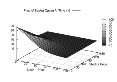
Figure 2. Basket option price of Example 4.3

References

• [1] Y. Achdou and O. Pironneau. Computational methods for option pricing. SIAM, Philadelphia, 2005.
• [2] T. J. I’a. Bromwich. Normal coordinates in dynamical systems. Proc. Lond. Math. Soc., 15(Ser. 2):401–448, 1916.
• [3] A. M. Cohen. Numerical methods for Laplace transform inversion. Springer, New York, 2007.
• [4] M. Crouzeix, S. Larsson, and V. Thomée. Resolvent estimates for elliptic finite element operators in one dimension. Math. Comp., 63:121–140, 1994.
• [5] K. S. Crump. Numerical inversion of Laplace transforms using a Fourier series approximation. J. ACM, 23(1):89–96, 1976.
• [6] D. I. Cruz-Báez and J. M. González-Rodriguez. A different approach for pricing European options. In MATH’05: Proceedings of the 8th WSEAS International Conference on Applied Mathematics, pages 373–378, Stevens Point, Wisconsin, USA, 2005. World Scientific and Engineering Academy and Society (WSEAS).
• [7] M. C. Fu, D. B. Madan, and T. Wang. Pricing continuous Asian options: a comparison of Monte Carlo and Laplace transform inversion methods. Journal of Computational Finance, 2:49–74, 1998.
• [8] I. P. Gavrilyuk, , W. Hackbusch, and B. N. Khoromskij. $\mathcal{H}$-matrix approximation for the operator exponential with applications. Numer. Math., 92:83–111, 2002.
• [9] I. P. Gavrilyuk, W. Hackbusch, and B. N. Khoromskij. Data-sparse approximation to a class of operator-valued functions. Math. Comp., 74(250):681–708 (electronic), 2005.
• [10] P. Glasserman. Monte Carlo Methods in Financial Engineering. Springer, 2003.
• [11] M. Griebel. A domain decomposition method using sparse grids. In Domain Decomposition Methods in Science and Engineering: The Sixth International Conference on Domain Decomposition, volume 157 of Contemporary Mathematics, pages 255–261, Providence, Rhode Island, 1994. American Mathematical Society.
• [12] R. Kangro and R. Nicolaides. Far field boundary conditions for Black-Scholes equations. SIAM J. Numer. Anal., 38:1357–1368, 2000.
• [13] J. Lee and D. Sheen. An accurate numerical inversion of Laplace transforms based on the location of their poles. Comput & Math. Applic., 48(10–11):1415–1423, 2004
• [14] J. Lee and D. Sheen. A parallel method for backward parabolic problems based on the Laplace transformation. SIAM J. Numer. Anal., 44:1466–1486, 2006.
• [15] C. C. W. Leentvaar and C. W. Oosterlee. Pricing multi-asset options with sparse grids and fourth order finite differences. In Numerical mathematics and advanced applications, pages 975–983. Springer, Berlin, 2006.
• [16] C.C.W. Leentvaar and C.W. Oosterlee. On coordinate transformation and grid stretching for sparse grid pricing of basket options. J. Comput. Appl. Math., 222(1):193–209, 2008.
• [17] M. López-Fernández and C. Palencia. On the numerical inversion of the laplace transform of certain holomorphic mappings. Appl. Numer. Math., 51:289–303, 2004.
• [18] R. Mallier and G. Alobaidi. Laplace transforms and American options. Applied Mathematical Finance, 7(4):241–256, December 2000.
• [19] A.-M. Matache, C. Schwab, and T. P. Wihler. Fast numerical solution of parabolic integrodifferential equations with applications in finance. SIAM J. Sci. Comput., 27(2):369–393 (electronic), 2005.
• [20] A.-M. Matache, T. von Petersdorff, and C. Schwab. Fast deterministic pricing of options on Lévy driven assets. M2AN Math. Model. Numer. Anal., 38(1):37–71, 2004.
• [21] W. McLean, I. H. Sloan, and V. Thomée. Time discretization via Laplace transformation of an integro-differential equation of parabolic type. Numer. Math., 102:497–522, 2006.
• [22] W. McLean and V. Thomée. Time discretization of an evolution equation with Laplace transforms. IMA J. Numer. Anal., 24:439–463, 2004.
• [23] A. Murli and M. Rizzardi. Algorithm 682: Talbot’s method for the Laplace inversion problem. ACM Trans. Math. Software, 16:158–168, 1990.
• [24] R. Panini and R. P. Srivastav. Pricing perpetual options using Mellin transforms. Appl. Math. Lett., 18:471–474, April 2005.
• [25] A. Pelsser. Pricing double barrier options using Laplace transforms. Finance and Stochastics, 4(1):95–104, 2000.
• [26] W. H. Press, S. A. Teukolsky, W. T. Vetterling, and B. P. Flannery. Numerical recipes in Fortran 90, volume 2 of Fortran Numerical Recipes. Cambridge University Press, Cambridge, second edition, 1996.
• [27] C. Reisinger and G. Wittum. Efficient hierarchical approximation of high-dimensional option pricing problems. SIAM J. Sci. Comput., 29(1):440–458 (electronic), 2007.
• [28] R. U. Seydel. Tools for Computational Finance. Springer, second edition, 2003.
• [29] D. Sheen, I. H. Sloan, and V. Thomée. A parallel method for time-discretization of parabolic problems based on contour integral representation and quadrature. Math. Comp., 69(229):177–195, 2000.
• [30] D. Sheen, I. H. Sloan, and V. Thomée. A parallel method for time-discretization of parabolic equations based on Laplace transformation and quadrature. IMA J. Numer. Anal., 23(2):269–299, 2003.
• [31] A. Talbot. The accurate numerical inversion of Laplace transforms. J. Inst. Maths. Applics., 23:97–120, 1979.
• [32] D. Tavella and C. Randall. Pricing Financial Instruments: The Finite Difference Method. Wiley, 2000.
• [33] V. Thomée. A high order parallel method for time discretization of parabolic type equations based on Laplace transformation and quadrature. Int. J. Numer. Anal. Model., 2:121–139, 2005.
• [34] T. von Petersdorff and C. Schwab. Numerical solution of parabolic equations in high dimensions. M2AN Math. Model. Numer. Anal., 38(1):93–127, 2004.
• [35] W. T. Weeks. Numerical inversion of Laplace transforms using Laguerre functions. J. ACM, 13(3):419–429, 1966.
• [36] J. A. C. Weideman. Algorithms for parameter selection in the Weeks method for inverting Laplace transforms. SIAM J. Sci. Comput., 21(1):111–128, 1999.
• [37] J. A. C. Weideman and L. N. Trefethen. Prabolic and hyperbolic contours for computing the Bromwich integral. Math. Comp., 76(259):1341–1356, Mar 2007.
• [38] D. V. Widder. The Laplace transform. Princeton University Press, Princeton, N.J., 1941.