Density Gradient Corrected Embedded Atom Method

Abstract

Through detailed comparisons between Embedded Atom Method (EAM) and first-principles calculations for Al, we find that EAM tends to fail when there are large electron density gradients present. We attribute the observed failures to the violation of the uniform density approximation (UDA) underlying EAM. To remedy the insufficiency of UDA, we propose a gradient-corrected EAM model which introduces gradient corrections to the embedding function in terms of exchange-correlation and kinetic energies. Based on the perturbation theory of “quasiatoms” and density functional theory, the new embedding function captures the essential physics missing in UDA, and paves the way for developing more transferable EAM potentials. With Voter-Chen EAM potential as an example, we show that the gradient corrections can significantly improve the transferability of the potential.

I Introduction

Atomistic simulations have become an increasingly powerful tool in materials research and a worthy partner of theory and experiment. Among the great many atomistic models, the Embedded Atom Method (EAM) eam ; meam has emerged as one of the most successful and versatile approaches, representing the mainstay of empirical atomistic simulations. To date, EAM has been applied to a variety of material systems, such as liquids, metals and alloys, semiconductors, ceramics, polymers, nano-structures, and composite materials. Examples of problems that EAM has studied include structure, energetics and dynamics of lattice defects,intro1 ; intro2 ; intro3 elastic response and phonons,intro4 ; intro5 ; intro6 fracture and plastic deformation,intro7 ; intro8 ; intro9 surface and surface growth,intro10 ; intro12 ; intro13 ; intro14 thermodynamics properties,intro15 and phase transitions,intro16 etc. The applications of EAM simulations have been reviewed in Ref. intro17, . The success and popularity of EAM are a consequence of its sound theoretical foundation - the density functional theory (DFT) and its simple analytical expression. The former assures that the essential physics be captured by EAM and the latter endows EAM with excellent numerical efficiency, in par with pair potentials.

Despite its great success, EAM suffers from a major deficiency - the lack of transferability. Most of EAM models are only reliable in regimes for which they were parameterized; beyond the regimes of parametrization, the reliability of EAM potentials quickly deteriorates. As a result, the predicability of EAM is often questionable in defect systems and in non-equilibrium conditions where relevant physical quantities are not known accurately a priori and hence not included in the parametrization of the potentials. As to all empirical models, the lack of transferability of EAM is an indication that some theoretical approximations of EAM model are not generally valid.

In this paper, we show that the lack of transferability of EAM is attributable to the uniform background density approximation of EAM embedding function. We find that EAM fails whenever there are large gradients of electron density in the system. We overcome the deficiency of the uniform density approximation (UDA) by proposing a density gradient corrected EAM model which incorporates the gradients of the valence electronic density in the embedding function. Specifically, we introduce additional terms into the embedding function which correspond to the density gradient corrections to the exchange-correlation and kinetic energy contributions. Motivated by the Perdew-Burke-Ernzerhof (PBE) pbe Generalized Gradient Approximation (GGA) of DFT and the perturbation theory of “quasiatoms” quasiatom , the present model applies to an inhomogeneous background density and has the correct limiting behavior as the exact energy functions. As a consequence, it extends the applicability of EAM and paves the way for developing more transferable potentials.

II Failures of the uniform density approximation

First, we demonstrate that the failure of EAM can be linked to the presence of large gradients of electron density by comparing EAM with first-principles DFT calculations. We establish this fact in bulk Al for which EAM is supposed to work very well. Several excellent EAM potentials ea ; mfmp ; vc exist and they are used for comparisons. Both elastic properties and stacking fault energy of Al are calculated. We compute the cohesive energy per atom and the stress tensor as a function of the right Cauchy-Green deformation tensor $C_{ij}$ ($i,j=1,2,3$) for a primitive unit cell of bulk Al. There are six independent $C$ elements, with the diagonal and off-diagonal elements varying from -0.28 to 0.28 and -0.18 to 0.18, respectively, giving rise to different elastic deformations. In order to provide precise comparisons, we utilize the sparse grid method spg - a novel algorithm that allows us to represent a fine high-dimensional mesh very efficiently. Specifically, we sample 483,201 data points in sparse grids which correspond to a regular grid with 65 points in each of the six dimensions of $C_{ij}$ and $65^{6}\approx 7.5\times 10^{10}$ points in total. Moreover, by taking advantage of the underlying symmetry of the system, we further reduce the number of data points from 483,201 to 24,567 for which we carry out first-principles and EAM calculations.

The first-principles DFT calculations are based on the plane-wave and Projector Augmented-Wave method paw as implemented in the Vienna Ab initio Simulation Package (VASP) vasp1 ; vasp2 . We use PBE-GGA with a high plane-wave cutoff energy of 360 eV to obtain reliable energy and stress. The $k$-points are sampled according to Monkhorst-Pack method with the $k$-point spacing less than 0.0252 Å^-1. A Gaussian smearing of 0.1 eV is employed to speed up the convergence of the calculations. As for EAM calculations, we employ three widely used EAM potentials, developed by Ercolessi and Adams ea , Mishin et al. mfmp , and Voter and Chen vc . The first two potentials were constructed by fitting to both experimental and first-principles data, while Voter-Chen potential was fitted only to experimental data. Although some EAM potentials ea were constructed with different motivations from the original EAM model, they all use the UDA in effect. For the convenience of presentation, we define $\Delta V=\frac{V-V_{0}}{V_{0}}$ and $\Delta\Omega=\frac{\Omega-\Omega_{0}}{\Omega_{0}}$, where $V$ ($V_{0}$) and $\Omega$ ($\Omega_{0}$) are the volume and solid angle of the deformed (undeformed) unit cell. The solid angle is defined relative to the basis vectors of the unit cell. $\Delta V$ and $\Delta\Omega$ characterize the volumetric and non-volumetric deformation of the unit cell.

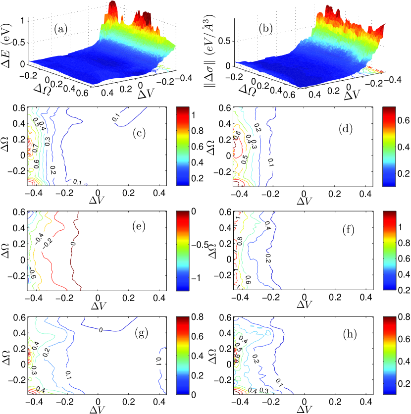
Figure 1: The difference for the elastic properties calculated by EAM and VASP. (a), (c), (e), and (g) show the cohesive energy differences in eV/atom; (b), (d), (f), and (h) show the stress differences in eV/ų. (a), (b), (c), and (d) are calculated by Ercolessi-Adams potential. (c) and (d) are the corresponding contour plots of (a) and (b), respectively. (e) and (f) are calculated by Mishin potential and (g) and (h) are calculated by Voter-Chen potential. (e), (f), (g), and (h) are contour plots.

In Figure 1, we present the difference in the cohesive energy $\left(\Delta E=E_{{\rm EAM}}-E_{{\rm VASP}}\right)$ and the stress tensor $\left(\left\|{\Delta\sigma}\right\|=\left\|{\sigma_{\rm EAM}-\sigma_{\rm VASP}}\right\|\right)$. Overall, we find excellent agreement between the first-principles and EAM results over a wide range of deformations - a remarkable feat of EAM. Furthermore, the errors are insensitive to the solid angle, $\Delta\Omega$, which reflects the delocalized nature of the metallic bonds in Al, and thus justify the use of an angular - independent model in Al. On the other hand, we find that the EAM errors depend very sensitively on the change of volume, $\Delta V$; in particular, the EAM values deviate significantly from the first-principles results for large compressions. The errors in energy can reach as high as 1 eV/atom for 40% compression. This dramatic difference cannot be accounted for by the fitting errors of EAM because all three potentials show exactly the same behavior. Moreover, the shortest interatomic distance in the compressed unit cell is 2.1 Å, which is still within the fitting range of the potentials. For example, the fitting range of bond length is from 2.0 Å to 6.3 Å in Mishin potential and 2.0 Å to 5.6 Å in Ercolessi-Adams potential. The results suggest that the errors come from the model itself.

When the interatomic distance decreases, the gradient of electronic density increases. For a large compression, the electron density gradient could become too large for the UDA of EAM to be valid. Indeed, we find that the density gradient increases considerably in compressions, with the maximum value of the gradients rising from 0.38 Å^-4 for the perfect lattice to 0.54 Å^-4 for 40% compression. On the other hand, the expansion of the lattice reduces the density gradient, and thus does not violate the UDA.

To further the argument, we perform additional calculations for the generalized stacking fault energy ($\gamma$) surface, which along with elastic constants, determines the plastic behavior of materials. We have carried out 293 energy calculations for the entire $\gamma$-surface with the sparse grid representation. The supercell consists of 9 layers in the $\left\langle{111}\right\rangle$ direction for both EAM and VASP calculations.

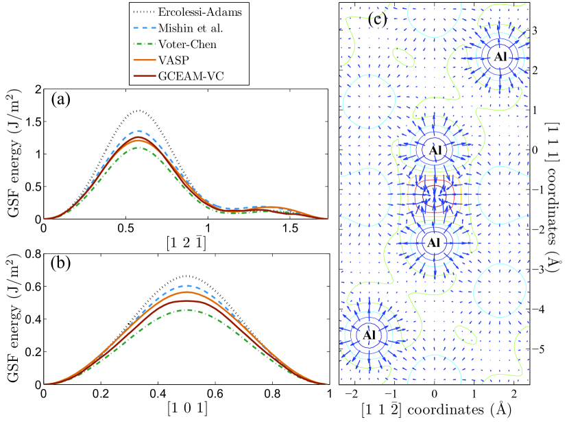
Figure 2: $\gamma$-energy along (a) $\left[12\bar{1}\right]$ and (b) $\left[101\right]$ directions from VASP and EAM calculations. The horizontal axis is in the unit of the Burgers vector of Al (2.86 Å). The contours of valence electronic density and the density gradient for the “run-on” configuration are shown in (c). The arrow represents the direction and magnitude of the density gradient.

The $\gamma$-energy along $[12\bar{1}]$ and $[101]$ directions is shown in Figure 2a and 2b. Again, overall agreement between the three EAM potentials and VASP is good. However, in the neighborhood of the [101] unstable stacking fault and the run-on stacking fault (the last two entries in Table 1), the magnitude of the energy error is significant. In particular, the largest error of EAM occurs at the run-on stacking fault in which the atoms in the two neighboring $\left(111\right)$ layers are right on top of each other, resulting in large density gradients. The valence electronic density and its gradient in the “run-on” configuration is presented in Figure 2c. Noted that the maximum gradient of valence electron density, $\left|g\right|_{\max}$ of both the unstable and the run-on stacking faults is comparable to the corresponding value of large compressions ($\sim 0.5$ Å^-4), suggesting that the failures of EAM can be indeed attributed to large density gradients, irrespective of the specific atomic configurations. Furthermore, the data in the brackets of the Table shows a general trend that the magnitude of EAM errors increases as the maximum density gradient increases. Again the shortest interatomic distance in Table 1 is 2.33 Å, which is within the fitting range of bond length for the EAM potentials.

Table 1: Fault vectors and energies for four stacking faults obtained from VASP and EAM calculations. All energies are in mJ/m². $\left|g\right|_{\max}$ denotes the maximum gradient of valence electronic density calculated by VASP, and is in Å^-4. PBE, EA, Mishin and Voter stand for the results calculated by VASP, Ercolessi-Adams, Mishin et al., and Voter-Chen EAM potential, respectively. The errors of EAM results are presented in brackets. $R_{\rm min}$ (Å) is the nearest neighbor distance in the corresponding configurations.

Vector	PBE	EA	Mishin	Voter	$\left|g\right|_{\max}$	$R_{\rm min}$
1/6[12$\bar{1}$]	111	121(10)	157(46)	87(-24)	0.398	2.86
1/10[12$\bar{1}$]	184	132(-56)	190(6)	118(-66)	0.399	2.74
1/4[101]	564	663(99)	603(39)	455(-109)	0.507	2.47
1/3[12$\bar{1}$]	1208	1667(459)	1354(146)	1096(-112)	0.581	2.33

III Density gradient correction model

Having established the importance of the density gradient, we propose a gradient corrected model which could potentially improve the transferability of EAM. The model is based on the pioneering work of Stott and Zaremba quasiatom on “quasiatoms”. Stott et al. have shown that by using a perturbation expansion for an inhomogeneous background density, the embedding energy of a “quasiatom” can be expressed rigorously as a function of the background density and its gradient. Based on the “quasiatoms” theory, we introduce three additional terms which account for the gradient corrections to the exchange, correlation and kinetic energy contributions to the embedding energy of EAM. In this context, the original embedding function of EAM can be regarded as the UDA to the embedding energy. Specifically, the corrected embedding function becomes

$$F_{i}\left({\bar{\rho}_{i},s_{i}}\right) = F_{0}\left(\bar{\rho}_{i}\right)+\tilde{F}_{C}\left(\bar{\rho}_{i}\right)g\left(s_{i}\right)$$ (1)

$$+\tilde{F}_{X}\left(\bar{\rho}_{i}\right)h\left(s_{i}\right)+\tilde{F}_{G}\left(\bar{\rho}_{i},s_{i}\right),$$

where $\bar{\rho}_{i}\equiv\sum\limits_{j\neq i}{\rho_{j}^{\rm at}(R_{ij})}$ is the background density at atom $i$, and $\rho^{\rm at}_{j}$ is the density contribution from atom $j$. $R_{ij}=\left|\vec{R}_{i}-\vec{R}_{j}\right|$ and $\vec{R}_{i}$ stands for the atomic coordinates. Although the background density $\bar{\rho}_{i}$ is not the same as the total density $\rho(\vec{r})$ where $\rho\left(\vec{r}\right)=\sum\limits_{j}{\rho_{j}^{\rm at}\left(\left|\vec{r}-\vec{R}_{j}\right|\right)}$, they are closely related and the gradients of both densities are well defined. In particular, we can define a dimensionless background density gradient $s_{i}$ as $s_{i}\propto{\left|\nabla_{\vec{R}_{i}}\bar{\rho}_{i}\right|}/{\bar{\rho}_{i}^{4/3}}$, where $\left|\nabla_{\vec{R}_{i}}\bar{\rho}_{i}\right|$ is the amplitude of background density gradient. In practice, $s_{i}$ can be approximated by its local average: $s_{i}\simeq\langle s_{i}\rangle\propto\frac{1}{\left[\bar{\rho}_{i}\right]^{4/3}}{\sum\limits_{j\neq i}\left|{\frac{\partial\rho_{j}^{\rm at}\left({R_{ij}}\right)}{\partial R_{ij}}}\right|}$. $F_{0}\left({\bar{\rho}}\right)$ is the UDA embedding function and $\tilde{F}_{G}$ is the gradient correction to the kinetic energy. The leading term of $\tilde{F}_{G}$ is of the von Weizsäcker form r14 , and can be approximated as $\tilde{F}_{G}\left(\bar{\rho},s\right)=\tilde{K}_{0}\left(\bar{\rho}\right)k\left(s\right)$. Here $\tilde{K}_{0}$ resembles the Thomas-Fermi kinetic energy tf1 ; tf2 and $k\left(s\right)=\lambda_{0}\frac{1+k_{11}s^{2}+k_{12}s^{4}}{1+k_{21}s^{2}+k_{22}s^{4}}s^{2}$. $\lambda_{0}$, $k_{11}$, $k_{12}$, $k_{21}$ and $k_{22}$ are undetermined parameters.

For exchange and correlation energy corrections, we adopt the functional form of PBE-GGA due to its simplicity. $\tilde{F}_{C}$ and $\tilde{F}_{X}$ in Equation 1 corresponds to the correlation and exchange energy of the local density approximation (LDA) of DFT and $g\left(s_{i}\right)$ and $h\left(s_{i}\right)$ are the corresponding gradient corrections. The explicit forms $\tilde{F}_{C}$ and $\tilde{F}_{X}$ can be found in standard references of LDA pz ; pw . We assume spin degeneracy here although the spin polarization can be considered easily and could be useful in the development of spin-dependent EAM potentials for magnetic materials. In addition, we require that the modified embedding functions have the same limiting behavior as the exact functions:

$$\left[g(s)\tilde{F}_{C}+h(s)\tilde{F}_{X}\right]\begin{cases}{\propto s^{2}\tilde{F}_{X},\hfill}&{s\to 0}\\ {\to-\tilde{F}_{C}+\kappa_{0}\tilde{F}_{X},\hfill}&{s\to\infty}\end{cases}.$$ (2)

We choose $g\left(s\right)=-\frac{{s}^{4}}{g_{0}+g_{1}{s}^{2}+{s}^{4}}$ and $h\left(s\right)=\frac{\kappa_{0}{s}^{2}}{1+\alpha{s}^{2}}$, which satisfy the above conditions although other forms of $g\left(s\right)$ and $h\left(s\right)$ can also be used.

Over all, there are six functions, $\tilde{F}_{C}$, $\tilde{F}_{X}$, $\tilde{K}_{0}$, $\rho^{\rm at}\left(R\right)$, $F_{0}\left(\rho\right)$, and $\varphi\left(R\right)$, which are to be fitted. The first three are new terms and in conjunction with $g\left(s\right)$, $h\left(s\right)$ and $k\left(s\right)$, they represent the gradient corrections to the embedding function.

Since the UDA functions, $\tilde{K}_{0}\left(\bar{\rho}\right)$, $\tilde{F}_{C}\left(\bar{\rho}\right)$, and $\tilde{F}_{X}\left(\bar{\rho}\right)$, have the same functional forms as their DFT/LDA counterpartstf1 ; tf2 ; pz ; pw , we have

$$\tilde{K}_{0}\left(\bar{\rho}\right)\propto\bar{\rho}^{5/3}.$$ (3a)

$$\tilde{F}_{C}\left(\bar{\rho}\right)=\bar{\rho}\left({c_{1}+c_{2}r_{s}}\right)\ln\left({1+\frac{1}{\beta r_{s}^{p+1}}}\right),\quad r_{s}\propto\frac{1}{\bar{\rho}^{1/3}},$$ (3b)

$$\tilde{F}_{X}\left(\bar{\rho}\right)\propto\bar{\rho}^{4/3},$$ (3c)

Replacing the proportional sign ‘$\propto$’ in all the above equations with an equal sign ‘=’, one can fit the gradient corrected EAM (GCEAM) potential by introducing 13 additional parameters. These additional parameters are $c_{1}$, $c_{2}$, $\beta$, $p$, $g_{0}$, $g_{1}$, $h_{0}$, $h_{1}$, $\lambda_{0}$, $k_{11}$, $k_{12}$, $k_{21}$, and $k_{22}$. Among them, seven parameters ($k_{11}$, $k_{12}$, $k_{21}$, $k_{22}$, $g_{0}$, $g_{1}$ and $\alpha$) are introduced through the gradient corrections. $\kappa_{0}$ and $\lambda_{0}$ can be absorbed into the embedding functions.

IV Example: Gradient Corrected Voter-Chen potential

In this section, we apply the gradient corrections to the Voter-Chen (VC) potential, and the resultant potential is termed as GCEAM-VC. It is important to mention that the corrections are not constrained in any way by the specific form of the EAM potential. We choose the VC potential because its simplicity - it has only five parameters, much fewer than other EAM potentials, such as Mishin and Ercolessi-Adams potentials. As a result, VC is not as accurate as the other EAM potentials. However, the simplicity of the VC potential renders more transparent physics, and frees us from intensive parameter fitting - which is not the emphasis of the present paper. The goal of the article is to illustrate the importance of the density gradient corrections in improving the transferability of EAM, rather than to generate the best possible EAM potential for Al. Had we started from an EAM potential with more parameters, we would have gotten even better test results for Al. Nevertheless, even with the VC potential, the gradient corrections can significantly improve the self-interstitial energies, stacking fault energies, etc. which involve high density gradient configurations.

The GCEAM-VC potential takes the general form of EAM model. The cohesive energy of a system can be written as

$$E=\frac{1}{2}\sum\limits_{i,j\left({\neq i}\right)}{\varphi_{ij}\left({R_{ij}}\right)+\sum\limits_{i}{F_{i}\left({\bar{\rho}_{i},s_{i}}\right)}},$$ (4)

where embedding function $F_{i}\left({\bar{\rho}_{i},s_{i}}\right)$ is expressed in Eq. (1).

The parameter fitting in GCEAM-VC follows the same procedure of the Voter-Chen potentialvc , but with two modifications. The first modification is that the pairwise interaction now is taken the form of:

$$\varphi\left(R\right) = \varphi_{1}\left(R\right)+\varphi_{2}\left(R\right),$$ (5)

$$\varphi_{1}\left(R\right) = D_{M}\left[{1-e^{-\alpha_{M}\left({R-R_{M}}\right)}}\right]^{2}-D_{M},$$

$$\varphi_{2}\left(R\right) = C\left({\frac{R_{M}}{R}}\right)^{n}.$$

Here, $\varphi_{1}\left(R\right)$ is a Morse potential used in the original Voter-Chen potential. $\varphi_{2}\left(R\right)$ is added to account for the repulsive interaction at short distance, $\varphi\left({R\to 0}\right)\to\infty$ when $C>0$. However, if one prefers to use fewer parameters, $\varphi_{2}\left(R\right)$ can be ignored without worsening the results (see the discussions of Fig. 4).

The second modification is that we do not fit the diatomic molecular data. Instead, the force constants of bulk Al with different lattice constants are fitted because accurate force constants give rise to accurate phonon dispersions, and hence, accurate thermal properties such as thermal capacity and conductivity. The force constants are fitted for several lattice constants, including 0.9$a_{0}$, 0.95$a_{0}$, $a_{0}$, 1.05$a_{0}$, and 1.1$a_{0}$, where $a_{0}$ is the equilibrium lattice constant of bulk Al. It is found the GCEAM-VC potential gives good description for the diatomic properties without fitting them (See Table II). This is an example of improved transferability of the GCEAM model.

The embedding function of both VC and GCEAM-VC potentials is determined by fitting the equation of states (EOS) to the universal EOS of Rose et al. EOS . Because the universal EOS does not agree exactly with the DFT (VASP) values (see Fig. 3), it is inevitable that both VC and GCEAM-VC potentials would deviate from DFT results for large lattice expansions or large interatomic distances. However, as shown later, the gradient corrections can improve significantly the description of high density gradient configurations involving lattice defects.

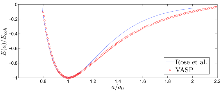
Figure 3: The cohesive energy per atom of fcc Al as a function of the lattice parameter (the scaled equation of states). $E_{coh}$ is the cohesive energy for equilibrium lattice constant $a_{0}$. The Rose et al.’s universal EOS is represented by the blue line, and the VASP values are represented by red open circles.

The density function of the VC potential is given as

$$\rho\left(r\right)=r^{6}\left[{e^{-\beta_{2}r}+2^{9}e^{-2\beta_{2}r}}\right],$$ (6)

$\beta_{2}$ needs to be fitted. We keep the same smoothness conditions for the pairwise interaction, atomic density and EOS function in GCEAM-VC as in the VC potential vc , with the cutoff radius $R_{\rm{cut}}$ of these functions to be fitted. Thus, there are seven parameters, $D_{M}$, $\alpha_{M}$, $R_{M}$, $C$, $n$, $\beta_{2}$ and $R_{\rm{cut}}$ to be fitted before applying the gradient corrections. Overall, there are twenty parameters in GCEAM-VC potential, including thirteen parameters associated with the gradient correction terms. The optimized values of all the parameters are presented in Table 2.

Table 2: One set of optimized parameters for GCEAM-VC. Length and energy unit are in $\AA$ and eV, respectively.

$c_{1}$	-0.45618	$g_{1}$	-1.60375	$k_{12}$	-58.09505	$R_{M}$	1.34426
$c_{2}$	-1.03903	$h_{0}$	0.41370	$k_{21}$	-10.15397	$C$	0.43750
$\beta$	1.17295	$h_{1}$	0.00327	$k_{22}$	26.82479	$n$	4.06038
$p$	0.29559	$\lambda_{0}$	-0.52795	$D_{M}$	4.00963	$\beta_{2}$	3.46742
$g_{0}$	1.63667	$k_{11}$	157.54365	$\alpha_{M}$	2.05403	$R_{\rm{cut}}$	5.56250

The pair interaction $\varphi(R)$ and the atomic density $\rho(R)$ of GCEAM-VC potential are plotted in Fig. 4 in comparison with the VC potential. It is found that the pair interaction of GCEAM-VC changes very little from that of VC. Although the atomic density function of GCEAM-VC potential appears to be rather different from that of VC, this turns out not to be the case. Using the fact that Eq. 4 is invariant under the transformation:

$$\rho\left(R\right)\to t\rho\left(R\right),F\left(\rho,s\right)\to F\left(\rho/t,s/t\right),$$

we can define a scaled atomic density $\tilde{\rho}\left(R\right)=\rho\left(R\right)/\max\left(\rho\left(R\right)\right)$. $\tilde{\rho}\left(R\right)$ is plotted in the bottom panel of Fig. 4 and one finds little difference between the GCEAM-VC and VC atomic density functions. Therefore, we conclude that all improvements to the VC potential come from the gradient corrections, i.e., the model itself.

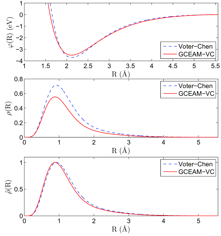
Figure 4: The pair interaction function $\varphi(R)$ and atomic density $\rho(R)$ of VC (blue dash) and GCEAM-VC (red solid) potentials.

Table 3: Properties of Al predicted by VC and and GCEAM-VC potentials in comparison with experimental and/or ab initio data. ^∗Fitted properties.

	Experimental or ab initio	Voter-Chen (Ref. vc, )	GCEAM-VC
Lattice properties:
$a_{0}$(Å)∗	4.05	4.05	4.05
$E_{0}$(eV/atom)∗	-3.36	-3.36	-3.36
$B$(GPa)∗	79	79	79.5
$c_{11}$(GPa)∗	114	107	113
$c_{12}$(GPa)∗	61.9	65.2	62.5
$c_{44}$(GPa)∗	31.6	32.2	32.9
Diatomic Properties:
$D_{e}$(eV)	1.60	1.54	1.61
$R_{e}$(Å)	2.47	2.45	2.52
Phonon frequencies:
$\nu_{L}\left(X\right)$(THz)	9.69	8.55	9.62
$\nu_{T}\left(X\right)$(THz)	5.80	5.20	5.36
$\nu_{L}\left(L\right)$(THz)	9.69	8.86	10.1
$\nu_{T}\left(L\right)$(THz)	4.19	3.70	3.82
$\nu_{L}\left(K\right)$(THz)	7.59	6.87	7.69
$\nu_{T_{1}}\left(K\right)$(THz)	5.64	4.80	5.00
$\nu_{T_{2}}\left(K\right)$(THz)	8.65	7.76	8.69
Vacancy:
$E_{v}^{f}$(eV)	0.68	0.63	0.65
Self-interstitial:
$E_{I}^{f}\left({O_{h}}\right)$(eV)	$2.73$	2.10	2.41
$E_{I}^{f}\left({T_{d}}\right)$(eV)	$3.08$	2.55	2.87
$E_{I}^{f}\left({\left[{111}\right]\rm{dumbell}}\right)$(eV)	2.97	2.48	2.81
$E_{I}^{f}\left({\left[{110}\right]\rm{dumbell}}\right)$(eV)	2.76	2.12	2.38
$E_{I}^{f}\left({\left[{100}\right]\rm{dumbell}}\right)$(eV)	$2.53$	2.02	2.30
Melting temperature:
$T_{m}$(K)	933.6	593.5$\pm$10	672.5$\pm$10

Some important properties predicted by VC and GCEAM-VC potentials are collected in Table 3. From Table 3, it is found that the GCEAM-VC improves the overall performance of the VC potential, especially for high density gradient configurations, such as self-interstitials. The table clearly demonstrates the success and improved transferability of GCEAM-VC.

Although GCEAM-VC gives a better result for the melting temperature than VC, the deviation from the experimental value is still large. This is due to the fact that the melting process is associated with long-range interactions, whereas the density gradient corrections tend to be short-ranged. Therefore the gradient corrections are not expected to have significant effect on melting temperature. This is not an intrinsic problem of the GCEAM model because one could improve the melting temperature by fitting more accurately the long-range tails of the UDA functions, e.g., $\phi\left(R\right)$, $\rho^{\rm{at}}\left(R\right)$, and $F_{0}\left(\rho\right)$.

In Fig. 5, we compare the phonon dispersions between GCEAM-VC and VC, against the experimental data. It is found that GCEAM-VC predicts much better results than VC.

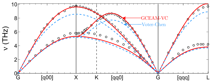
Figure 5: The phonon dispersion curves for Al. Red lines are calculated with GCEAM-VC potential, blue dash lines are calculated with VC potential, and open circles are experimental data taken from Ref. PhDisp, .

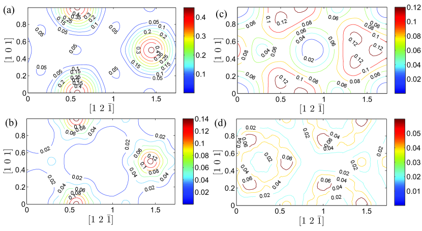
Figure 6: The absolute error between the $\gamma$-surface from EAM potentials and first-principles calculations $\left|E^{\rm EAM}_{\rm GSF}-E^{\rm VASP}_{\rm GSF}\right|$. In (a), (b), (c) and (d), the EAM potentials are Ercolessi-Adams, Mishin, VC and GCEAM-VC, respectively.

Furthermore, with the help of the sparse-grid method, we calculate the entire $\gamma$-surface using first-principles VASP method. From the $\gamma$-surface, one can derive the properties of all $\{111\}$-type dislocations in Al GammaSuf . The absolute errors between the $\gamma$-surface determined by various EAM potentials and VASP calculations are shown in Fig. 6. The projection of the $\gamma$-surface along two special orientations is plotted in Figure 2a and 2b. It is found that the GCEAM-VC potential yields the most accurate result for overall $\gamma$-surface. Here we should emphasize that GCEAM-VC does not fit any stacking fault configurations. In contrast, Ercolessi-Adams and Mishin et al. potentials both have included $\gamma$-energies in their fitting database, and yet their results are not as good as GCEAM-VC. This is an important success of GCEAM potential in terms of transferability. Moreover, GCEAM-VC potential gives much more accurate stacking fault energy near the “run-on” configuration ($\left({\frac{\sqrt{3}}{3},0}\right)$, $\left({\frac{\sqrt{3}}{3},1}\right)$, and $\left({\frac{5\sqrt{3}}{6},\frac{1}{2}}\right)$ in Fig. 6). These results confirm that indeed the gradient corrections are crucial for describing high density gradient configurations, such as the “run-on” stacking faults. On the other hand, the errors of GCEAM-VC appear at configurations where interatomic distance is greater than that of a perfect lattice. These errors are not the intrinsic problem of the gradient correction model, but rather due to the fitting strategy of the Voter-Chen potential.

Finally, it is useful to mention that the force calculation in GCEAM maintains the comparable numerical efficiency with the standard EAM models. Thanks to the fact that the modified embedding functions can be factored by a $\rho$-dependent term and an $s$-dependent term, the analytical expression of force remains simple - it has several additional terms that are of similar complexity of that of standard EAM. To compute these additional terms, the GCEAM needs to perform extra calculations of which the most time-consuming part is the second derivatives of the charge density with respect to distance. By using cubic spline interpolations, these calculations can be made rather efficient and as a result, the GCEAM force calculation takes less than twice of the CPU time of the standard EAM. The code package for calculating the energy and force with GCEAM-VC potential is available via the World Wide Webwebsite or via e-mail at wugaxp@gmail.com.

V Discussion and Conclusion

Finally, it is instructive to relate the present corrections to other EAM models meam ; msmeam ; cteam . In the original EAM model, the electron correlations arising from the inhomogeneous background density are largely ignored. The goal of the present model is to capture the missing correlations by taking into consideration of density gradients. Apart from the inhomogeneity of the density, the correlation effect also manifests itself in small molecules and clusters - a well-known fact in quantum chemistry that motivated the development of GGAs. By introducing a PBE GGA-like correction to the exchange-correlation part of the embedding energy, the present model could improve the description of the correlation effect. The modified EAM (MEAM) and its multistate variant strive to improve the transferability by making the background density $\bar{\rho}$ angular and reference-state dependent. However, since they are based on UDA, the MEAM model does not treat the electron correlations adequately. As a result, it cannot deal with small clusters accurately as documented in the literature meam_89 . The charge transfer EAM (CT-EAM) also recognizes the importance of the correlation effect. However it addresses the problem by introducing a reference-state (and its charge) dependent background density $\bar{\rho}$. Since the present model considers exchange-correlation energy explicitly, it can achieve the same goal of CT-EAM with a simpler function form. Moreover, one could incorporate MEAM and its variants into the present model by making the background density $\bar{\rho}$ in Eq. (1) as angular, reference-state and/or charge-dependent if so desired.

In conclusion, we have performed detailed EAM and first-principles calculations of Al for elastic deformation and generalized stacking fault energy. We find that although EAM models reproduce well the first-principles results for most cases, they tend to fail when the electron density gradients become substantial. We attribute the failures of EAM to the violation of UDA underlying the existing EAM models. To remedy the deficiency of UDA, we propose an improved EAM model which considers explicitly the gradient corrections to the embedding function in terms of the exchange-correlation energy and the kinetic energy. We show that the gradient corrected model can significantly improve the transferability of EAM, and represents a new direction for developing more transferable EAM potentials.

- (1) M.S. Daw and M.I. Baskes, Phys. Rev. Lett. 50, 1285 (1983); Phys. Rev. B 29, 6443 (1984).
- (2) M.I. Baskes, Phys. Rev. Lett. 59, 2666 (1987); Phys. Rev. B 46, 2727 (1992).
- (3) S.M. Foiles, M.I. Baskes and M.S. Daw, Phys. Rev. B 33, 7983 (1986); ibid. 37, 10378 (1988).
- (4) J.B. Adams, S.M. Foiles and W.G. Wolfer, J. Mater. Res. 4, 102 (1989).
- (5) A.D. LeClaire, J. Nucl. Mater. 69/70, 70 (1978).
- (6) M.S. Daw and R.D. Hatcher, Solid State Commun. 56, 697 (1985).
- (7) J.S. Nelson, M.S. Daw and E.C. Sowa, Phys. Rev. B 40, 1465 (1989).
- (8) J.S. Nelson, E.C. Sowa and M.S. Daw, Phys. Rev. Lett. 61, 1977 (1988).
- (9) M.I. Baskes and M.S. Daw, in: Fourth International Conference on the Effect of Hydrogen on the Behavior of Materials, Jackson Lake Lodge, Moran, WY, eds. N. Moody and A. Thompson (The Minerals, Metals, and Materials Society, Warrendale, PA, 1989).
- (10) R.G. Hoagland, M.S. Daw, S.M. Foiles and M.I. Baskes, in: Atomic Scale Calculations of Structure in Materials, eds. M.S. Daw and M.A. Schliiter (Materials Research Society, Pittsburgh, PA, 1990).
- (11) R.G. Hoagland, M.S. Daw and J.P. Hirth, J. Mater. Res. 6, 2565 (1991).
- (12) S.P. Chen, A. Voter and D.L. Srolovitz, Phys. Rev. Lett. 57, 1308 (1986).
- (13) S.P. Chen, D.J. Srolovitz and A.F. Voter, J. Mater. Res. 4, 62 (1989).
- (14) T. Ning, Q. Yu and Y. Ye, Surface Sci. 206, L857 (1988).
- (15) K. Takahashi, C. Nara, T. Yamagishi, and T. Onzawa, Appl. Surf. Science 151, 299 (1999).
- (16) S.M. Foiles and M.S. Daw, Phys. Rev. B 38, 12643 (1988).
- (17) S.M. Foiles and J.B. Adams, Phys. Rev. B 40, 5909 (1989).
- (18) M. S. Daw, S. M. Foiles, and M. I. Baskes, Mater. Sci. Rep. 9, 251 (1993).
- (19) J. P. Perdew, K. Burke, and M. Ernzerhof, Phys. Rev. Lett. 77, 3865 (1996).
- (20) M.J. Stott and E. Zaremba, Phys. Rev. B 22, 1564 (1980).
- (21) F. Ercolessi and J. B. Adams, Europhys. Lett., 26 (8), 583 (1994).
- (22) Y. Mishin, D. Farkas, M. J. Mehl and D. A. Papaconstantopoulos, Phys. Rev. B 59, 3393 (1999).
- (23) A. Voter and S. Chen, Mat. Res. Soc. Symp. Proc. 82, 175 (1987).
- (24) H.-J. Bungartz and M. Griebel, Acta Numerica 13, 147 (2004).
- (25) G. Kresse and D. Joubert, Phys. Rev. B 59, 1758 (1999).
- (26) G. Kresse and J. Hafner, Phys. Rev. B 48, 13115 (1993).
- (27) G. Kresse and J. Furthmüller, Comput. Mater. Sci. 6, 15 (1996); Phys. Rev. B 54, 11 169 (1996).
- (28) C. F. von Weizsäcker, Z. Phys. 96, 431 (1935); D. A. Kirzhnits, Sov. Phys. JETP 5, 64 (1957).
- (29) L.H. Thomas, Proc. Cambridge philos. Soc. 23, 542 (1926).
- (30) E.Fermi, Z.Phys. 48, 73 (1928).
- (31) J. P. Perdew and A. Zunger, Phys. Rev. B 23, 5048 (1981).
- (32) J. P. Perdew and Y. Wang, Phys. Rev. B 45, 13244 (1992).
- (33) J.H. Rose, J.R. Smith, F. Guinea, and J. Ferrante, Phys. Rev. B 29, 2963 (1984).
- (34) C. Kittel, Introduction to Solid State Physics (Wiley-Interscience, New York, 1986).
- (35) Handbook of Chemistry and Physics, edited by R. C. Weast (CRC, Boca Raton, FL, 1984).
- (36) G. Simons and H. Wang, Single Crystal Elastic Constants and Calculated Aggregate Properties (MIT Press, Cambridge, MA, 1977).
- (37) K.P. Huber and G. Hertzberg, Constants of Diatomic Molecules (Van Nostrand Reinhold, New York, 1979).
- (38) R. Stedman and G. Nilsson, Phys. Rev. 145, 492 (1966).
- (39) H.-E. Schaefer, R. Gugelmeier, M. Schmolz, and A. Seeger, Mater. Sci. Forum 15-18, 111 (1987).
- (40) R. Stedman and G. Nilsson, Phys. Rev. 145, 492 (1966).
- (41) G. Lu, N. Kioussis, V.V. Bulatov, and E. Kaxiras, Phys. Rev. B 62, 3099 (2000).
- (42) http://wugaxp.com/Documents/GCEAM-VC.tar.gz.
- (43) M.I. Baskes, S. G. Srinivasan, S. M. Valone, and R.G. Hoagland, Phys. Rev. B 75, 094113 (2007).
- (44) S. M. Valone and S.R. Atlas, Philos. Mag. 86, 2683 (2006).
- (45) M.I. Baskes, J.S. Nelson and A.F. Wright, Phys. Rev. B 40, 6085 (1989).