Biological Network Comparison Using Graphlet Degree Distribution

Abstract

1 Motivation:

Analogous to biological sequence comparison, comparing cellular networks is an important problem that could provide insight into biological understanding and therapeutics. For technical reasons, comparing large networks is computationally infeasible, and thus heuristics, such as the degree distribution, clustering coefficient, diameter, and relative graphlet frequency distribution have been sought. It is easy to demonstrate that two networks are different by simply showing a short list of properties in which they differ. It is much harder to show that two networks are similar, as it requires demonstrating their similarity in all of their exponentially many properties. Clearly, it is computationally prohibitive to analyze all network properties, but the larger the number of constraints we impose in determining network similarity, the more likely it is that the networks will truly be similar.

2 Results:

We introduce a new systematic measure of a network’s local structure that imposes a large number of similarity constraints on networks being compared. In particular, we generalize the degree distribution, which measures the number of nodes ‘‘touching’’ $k$ edges, into distributions measuring the number of nodes ‘‘touching’’ $k$ graphlets, where graphlets are small connected non-isomorphic subgraphs of a large network. Our new measure of network local structure consists of $73$ graphlet degree distributions of graphlets with 2, 3, 4, and 5 nodes, but it is easily extendible to a greater number of constraints (i.e, graphlets), if necessary, and the extensions are limited only by the available CPU. Furthermore, we show a way to combine the $73$ graphlet degree distributions into a network ‘‘agreement’’ measure which is a number between $0$ and $1$, where $1$ means that networks have identical distributions and $0$ means that they are far apart. Based on this new network agreement measure, we show that almost all of the fourteen eukaryotic PPI networks, including human, resulting from various high-throughput experimental techniques, as well as from curated databases, are better modeled by geometric random graphs than by Erdos-Renyi, random scale-free, or Barabasi-Albert scale-free networks.

3 Availability:

Software executables are available upon request.

4 Contact:

natasha@ics.uci.edunatasha@ics.uci.edu

5 Introduction

Understanding cellular networks is a major problem in current computational biology. These networks are commonly modeled by graphs (also called networks) with nodes representing biomolecules such as genes, proteins, metabolites etc., and edges representing physical, chemical, or functional interactions between the biomolecules. The ability to compare such networks would be very useful. For example, comparing a diseased cellular network to a healthy one may aid in finding a cure for the disease, and comparing cellular networks of different species could enable evolutionary insights. A full description of the differences between two large networks is infeasible because it requires solving the subgraph isomorphism problem, which is an NP-complete problem. Therefore, analogous to the BLAST heuristic (Altschul90, ) for biological sequence comparison, we need to design a heuristic tool for the full-scale comparison of large cellular networks (Berg04, ). The current network comparisons consist of heuristics falling into two major classes: 1) global heuristics, such as counting the number of connections between various parts of the network (the ‘‘degree distribution’’), computing the average density of node neighborhoods (the ‘‘clustering coefficients’’), or the average length of shortest paths between all pairs of nodes (the ‘‘diameter’’); and 2) local heuristics that measure relative distance between concentrations of small subgraphs (called graphlets) in two networks (Przulj04, ).

Since cellular networks are incompletely explored, global statistics on such incomplete data may be substantially biased, or even misleading with respect to the (currently unknown) full network. Conversely, certain neighborhoods of these networks are well-studied, and so locally based statistics applied to the well-studied areas are more appropriate. A good analogy would be to imagine that MapQuest knew details of the streets of New York City and Los Angeles, but had little knowledge of highways spanning the country. Then, it could provide good driving directions inside New York or L. A., but not between the two. Similarly, we have detailed knowledge of certain local areas of biological networks, but data outside these well-studied areas is currently incomplete, and so global statistics are likely to provide misleading information about the biological network as a whole, while local statistics are likely to be more valid and meaningful.

Due to the noise and incompleteness of cellular network data, local approaches to analyzing and comparing cellular network structure that involve searches for small subgraphs have been successful in analyzing, modeling, and discovering functional modules in cellular networks (Milo02, ; Shen-Orr02, ; Milo04, ; Przulj04, ). Note that it is easy to show that two networks are different simply by finding any property in which they differ. However, it is much harder to show that they are similar, since it involves showing that two networks are similar with respect to all of their properties. Current common approaches to show network similarity are based on listing several common properties, such as the degree distribution, clustering, diameter, or relative graphlet frequency distribution. The larger the number of common properties, the more likely it is that the two networks are similar. But any short list of properties can easily be mimicked by two very large and different networks. For example, it is easy to construct networks with exactly the same degree distribution whose structure and function differ substantially (Przulj04, ; Li05, ; Doyle05, ).

In this paper, we design a new local heuristic for measuring network structure that is a direct generalization of the degree distribution. In fact, the degree distribution is the first in the spectrum of $73$ graphlet degree distributions that are components of this new measure of network structure. Thus, in our new network similarity measure, we impose $73$ highly structured constraints in which networks must show similarity to be considered similar; this is a much larger number of constraints than provided by any of the previous approaches and therefore it increases the chances that two networks are truly similar if they are similar with respect to this new measure. Moreover, the measure can be easily extended to a greater number of constraints simply by adding more graphlets. The extensions are limited only by the available CPU.

Based on this new measure of structural similarity between two networks, we show that the geometric random graph model shows exceptionally high agreement with twelve out of fourteen different eukaryotic protein-protein interaction (PPI) networks. Furthermore, we show that such high structural agreements between PPI and geometric random graphs are unlikely to be beaten by another random graph model, at least under this measure.

5.1 Background

Large amounts of cellular network data for a number of organisms have recently become available through high-throughput methods (Ito00, ; uetz00, ; GiotSci03, ; Vidal04, ; Stelzl05, ; Rual05, ). Statistical and theoretical properties of these networks have been extensively studied (Jeong00, ; Maslov02, ; Shen-Orr02, ; Milo02, ; Vazquez04, ; Yeger-Lotem04, ; Przulj04, ; Tanaka05, ) due to their important biological implications (Jeong01, ; LappeHolm04, ).

Comparing large cellular networks is computationally intensive. Exhaustively computing the differences between networks is computationally infeasible, and thus efficient heuristic algorithms have been sought (Kashtan04, ; Przulj06, ). Although global properties of large networks are easy to compute, they are inappropriate for use on incomplete networks because they can at best describe the structure produced by the biological sampling techniques used to obtain the partial networks (Vidal05, ). Therefore, bottom-up or local heuristic approaches for studying network structure have been proposed (Milo02, ; Shen-Orr02, ; Przulj04, ). Analogous to sequence motifs, network motifs have been defined as subgraphs that occur in a network at frequencies much higher than expected at random (Milo02, ; Shen-Orr02, ; Milo04, ). Network motifs have been generalized to topological motifs as recurrent ‘‘similar’’ network sub-patterns (Berg04, ). However, the approaches based on network motifs ignore infrequent subnetworks and subnetworks with ‘‘average’’ frequencies, and thus are not sufficient for full-scale network comparison. Therefore, small connected non-isomorphic induced subgraphs of a large network, called graphlets, have been introduced to design a new measure of local structural similarity between two networks based on their relative frequency distributions (Przulj04, ).

The earliest attempts to model real-world networks include Erdos-Renyi random graphs (henceforth denoted by ‘‘ER’’) in which edges between pairs of nodes are distributed uniformly at random with the same probability $p$ (ErdosRenyi59, ; ErdosRenyi60, ). This model poorly describes several properties of real-world networks, including the degree distribution and clustering coefficients, and therefore it has been refined into generalized random graphs in which the edges are randomly chosen as in Erdos-Renyi random graphs, but the degree distribution is constrained to match the degree distribution of the real network (henceforth we denote these networks by ‘‘ER-DD’’). Matching other global properties of the real-world networks to the model networks, such as clustering coefficients, lead to further improvements in modeling real-world networks including small-world (Watts-Strogatz98, ; Newman99a, ; Newman99b, ) and scale-free (Simon55, ; Barabasi99, ) network models (henceforth, we denote by ‘‘SF’’ scale-free Barabasi-Albert networks). Many cellular networks have been described as scale-free (Barabasi_Oltvai04, ). However, this issue has been heavily debated (Aguiar05, ; Stumpf05, ; Vidal05, ; Tanaka05, ). Recently, based on the local relative graphlet frequency distribution measure, a geometric random graph model (Penrose03, ) has been proposed for high-confidence PPI networks (Przulj04, ).

6 Approach

In section 6.1, we describe the fourteen PPI networks and the four network models that we analyzed. Then we describe how we generalize the degree distribution to our spectrum of graphlet degree distributions (section 6.2); note that the degree distribution is the first distribution in this spectrum, since it corresponds to the only graphlet with two nodes. Finally, we construct a new measure of similarity between two networks based on graphlet degree distributions (section 6.3). We describe the results of applying this measure to the fourteen PPI networks in section 7.

6.1 PPI and Model Networks

We analyzed PPI networks of the eukaryotic organisms yeast S. cerevisiae, frutifly D. melanogaster, nematode worm C. elegans, and human. Several different data sets are available for yeast and human, so we analyzed five yeast PPI networks obtained from three different high-throughput studies (uetz00, ; Ito00, ; Mering02, ) and five human PPI networks obtained from the two recent high-throughput studies (Stelzl05, ; Rual05, ) and three curated data bases (Bader03, ; hprd, ; MINT, ). We denote by ‘‘YHC’’ the high-confidence yeast PPI network as described by Mering02, , by ‘‘Y11K’’ the yeast PPI network defined by the top $11,000$ interactions in the Mering02, classification, by ‘‘YIC’’ the Ito00, ‘‘core’’ yeast PPI network, by ‘‘YU’’ the uetz00, yeast PPI network, and by ‘‘YICU’’ the union of Ito00, core and uetz00, yeast PPI networks (we unioned them as did Vidal05, to increase coverage). ‘‘FE’’ and ‘‘FH’’ denote the fruitfly D. melanogaster entire and high-confidence PPI networks published by GiotSci03, . Similarly, ‘‘WE’’ and ‘‘WC’’ denote the worm C. elegans entire and ‘‘core’’ PPI networks published by Vidal04, . Finally, ‘‘HS’’, ‘‘HG’’, ‘‘HB’’, ‘‘HH’’, and ‘‘HM’’ stand for human PPI networks by Stelzl05, , Rual05, , from BIND (Bader03, ), HPRD (hprd, ), and MINT (MINT, ), respectively (BIND, HPRD, and MINT data have been downloaded from OPHID (Brown05, ) on February 10, 2006). Note that these PPI networks come from of a wide array of experimental techniques; for example, YHC and Y11K are mainly coming from tandem affinity purifications (TAP) and high throughput MS/MS protein complex identification (HMS-PCI), while YIC, YU, YICU, FE, FH, WE, WH, HS, and HG are yeast two-hybrid (Y2H), and HB, HH, and HM are a result of human curation (BIND, HPRD, and MINT).

The four network models that we compared against the above fourteen PPI networks are ER, ER-DD, SF, and 3-dimensional geometric random graphs (henceforth denoted by ‘‘GEO-3D’’). Model networks corresponding to a PPI network have the same number of nodes and the number of edges within $1\%$ of the PPI network’s (details of the construction of model networks are presented by Przulj04, ). For each of the fourteen PPI networks, we constructed and analyzed $25$ networks belonging to each of these four network models. Thus, we analyzed the total of $14+14\cdot 4\cdot 25=1,414$ networks. We compared the agreement of each of the fourteen PPI networks with each of the corresponding $4\cdot 25=100$ model networks described above (our new agreement measure is described in section 6.3). The results of this analysis are presented in section 7.

6.2 Graphlet Degree Distribution (GDD)

We generalize the notion of the degree distribution as follows. The degree distribution measures, for each value of $k$, the number of nodes of degree $k$. In other words, for each value of $k$, it gives the number of nodes ‘‘touching’’ $k$ edges. Note that an edge is the only graphlet with two nodes; henceforth, we call this graphlet $G_{0}$ (illustrated in Figure 1). Thus, the degree distribution measures the following: how many nodes ‘‘touch’’ one $G_{0}$, how many nodes ‘‘touch’’ two $G_{0}$s, $\ldots$, how many nodes ‘‘touch’’ $k$ $G_{0}$s. Note that there is nothing special about graphlet $G_{0}$ and that there is no reason not to apply the same measurement to other graphlets. Thus, in addition to applying this measurement to an edge, i.e., graphlet $G_{0}$, as in the degree distribution, we apply it to the twenty-nine graphlets $G_{1},G_{2},\ldots G_{29}$ presented in Figure 1 as well.

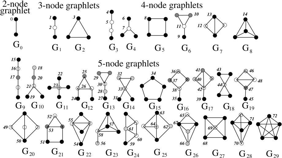
Figure 1: Automorphism orbits $0,1,2,\ldots,72$ for the thirty 2, 3, 4, and 5-node graphlets $G_{0},G_{1},\ldots,G_{29}$. In a graphlet $G_{i}$, $i\in\{0,1,\ldots 29\}$, nodes belonging to the same orbit are of the same shade.

When we apply this measurement to graphlets $G_{0},\ldots,G_{29}$, we need to take care of certain topological issues that we first illustrate in the following example and then define formally. For graphlet $G_{1}$, we ask how many nodes touch a $G_{1}$; however, note that it is topologically relevant to distinguish between nodes touching a $G_{1}$ at an end or at the middle node. This is due to the following mathematical property of $G_{1}$: a $G_{1}$ admits an automorphism (defined below) that maps its end nodes to each other and the middle node to itself. To understand this phenomenon, we need to recall the following standard mathematical definitions. An isomorphism $g$ from graph $X$ to graph $Y$ is a bijection of nodes of $X$ to nodes of $Y$ such that $xy$ is an edge of $X$ if and only if $g(x)g(y)$ is an edge of $Y$; an automorphism is an isomorphism from a graph to itself. The automorphisms of a graph $X$ form a group, called the automorphism group of $X$, and commonly denoted by $Aut(X)$. If $x$ is a node of graph $X$, then the automorphism orbit of $x$ is $Orb(x)=\{y\in V(X)|y=g(x)\text{ for some }g\in Aut(X)\}$, where $V(X)$ is the set of nodes of graph $X$. Thus, end nodes of a $G_{1}$ belong to one automorphism orbit, while the mid-node of a $G_{1}$ belongs to another. Note that graphlet $G_{0}$ (i.e., an edge) has only one automorphism orbit, as does graphlet $G_{2}$; graphlet $G_{3}$ has two automorphism orbits, as does graphlet $G_{4}$, graphlet $G_{5}$ has one automorphism orbit, graphlet $G_{6}$ has three automorphism orbits etc. (see Figure 1). In Figure 1, we illustrate the partition of nodes of graphlets $G_{0},G_{1},\ldots,G_{29}$ into automorphism orbits (or just orbits for brevity); henceforth, we number the $73$ different orbits of graphlets $G_{0},G_{1},\ldots,G_{29}$ from $0$ to $72$, as illustrated Figure 1. Analogous to the degree distribution, for each of these $73$ automorphism orbits, we count the number of nodes touching a particular graphlet at a node belonging to a particular orbit. For example, we count how many nodes touch one triangle (i.e., graphlet $G_{2}$), how many nodes touch two triangles, how many nodes touch three triangles etc. We need to separate nodes touching a $G_{1}$ at an end-node from those touching it at a mid-node; thus we count how many nodes touch one $G_{1}$ at an end-node (i.e., at orbit $1$), how many nodes touch two $G_{1}$s at an end-node, how many nodes touch three $G_{1}$s at an end-node etc. and also how many nodes touch one $G_{1}$ at a mid-node (i.e., at orbit $2$), how many nodes touch two $G_{1}$s at a mid-node, how many nodes touch three $G_{1}$s at a mid-node etc. In this way, we obtain $73$ distributions analogous to the degree distribution (actually, the degree distribution is the distribution for the $0^{th}$ orbit, i.e., for graphlet $G_{0}$). Thus, the degree distribution, which has been considered to be a global network property, is one in the spectrum of $73$ ‘‘graphlet degree distributions (GDDs)’’ measuring local structural properties of a network. Note that GDD is measuring local structure, since it is based on small local network neighborhoods. The distributions are unlikely to be statistically independent of each other, although we have not yet worked out the details of the inter-dependence.

6.3 Network ‘‘GDD Agreement’’

There are many ways to ‘‘reduce’’ the large quantity of numbers representing $73$ sample distributions. In this section, we describe one way; there may be better ways, and certainly finding better ways to reduce this data is an obvious future direction. Some of the details may seem obscure at first; we justify them at the end of this section.

We start by measuring the $73$ graphlet degree distributions (GDDs) for each network that we wish to compare. Let $G$ be a network (i.e., a graph). For a particular automorphism orbit $j$ (refer to Figure 1), let $d_{G}^{j}(k)$ be the sample distribution of the number of nodes in $G$ touching the appropriate graphlet (for automorphism orbit $j$) $k$ times. That is, $d_{G}^{j}$ represents the $j^{th}$ graphlet degree distribution (GDD). We scale $d_{G}^{j}(k)$ as

$$S_{G}^{j}(k)=\frac{d_{G}^{j}(k)}{k}$$ (1)

to decrease the contribution of larger degrees in a GDD (for reasons we describe later that are illustrated in Figure 2), and then normalize the distribution with respect to its total area,

$$T_{G}^{j}=\sum_{k=1}^{\infty}S_{G}^{j}(k).$$ (2)

giving the ‘‘normalized distribution’’

$$N_{G}^{j}(k)=\frac{S_{G}^{j}(k)}{T_{G}^{j}}.$$ (3)

In words, $N_{G}^{j}(k)$ is the fraction of the total area under the curve, over the entire GDD, devoted to degree $k$. Finally, for two networks $G$ and $H$ and a particular orbit $j$, we define the ‘‘distance’’ $D^{j}(G,H)$ between their normalized $j^{th}$ distributions as

$$D^{j}(G,H)=\left(\sum_{k=1}^{\infty}[N_{G}^{j}(k)-N_{H}^{j}(k)]^{2}\right)^{\frac{1}{2}},$$ (4)

where again in practice the upper limit of the sum is finite due to the finite sample. The distance is between $0$ and $1$, where $0$ means that $G$ and $H$ have identical $j^{th}$ GDDs, and $1$ means that their $j^{th}$ GDDs are far away. Next, we reverse $D^{j}(G,H)$ to obtain the $j^{th}$ GDD agreement:

$$A^{j}(G,H)=1-D^{j}(G,H),$$ (5)

for $j\in\{0,1,\ldots,72\}$. Finally, the agreement between two networks $G$ and $H$ is either the arithmetic (equation 6) or geometric (equation 7) mean of $A^{j}(G,H)$ over all $j$, i.e.,

$$A_{arith}(G,H)=\frac{1}{73}\sum_{j=0}^{72}A^{j}(G,H),$$ (6)

and

$$A_{geo}(G,H)=\left(\prod_{j=0}^{72}A^{j}(G,H)\right)^{\frac{1}{73}}.$$ (7)

(A)

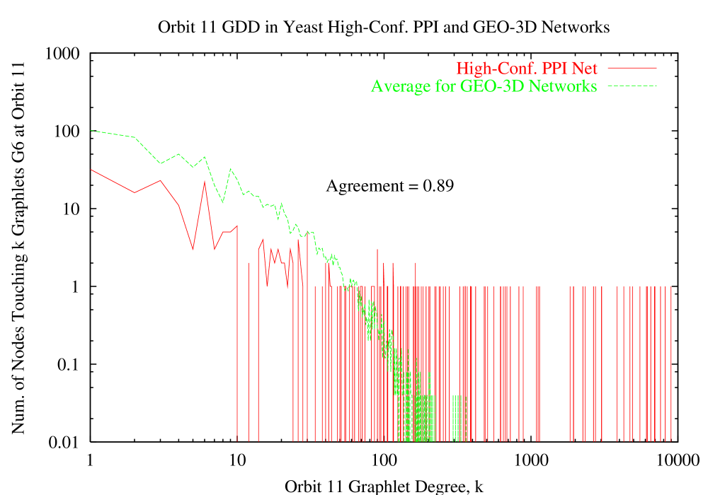
(B)

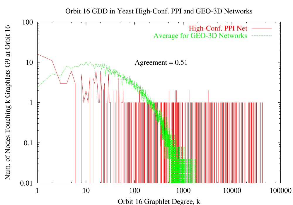
Figure 2: Examples of graphlet degree distributions (GDDs) for yeast high-confidence PPI network (Mering02, ) (solid red line) and the average of 25 corresponding 3-dimensional geometric random networks (GEO-3D, dashed green line): A. Orbit 11. B. Orbit 16. Most counts beyond about $k=20$ are zero, with a few instances of 1 or (very occasionally) 2. This results in a large amount of red and green ink which is mostly noise, as the distribution fluctuates frequently from 1 to 0 (which is $-\infty$ on our log scale). The noise could be reduced by applying a broad-band filter, but we have chosen to leave the data in its raw state, despite the deleterious effect on the aesthetics of the plot.

Now we give the rationale for designing the agreement measure in this way. There are many different ways to design a measure of agreement between two distributions. They are all heuristic, and thus one needs to examine the data to design the agreement measure that works best for a particular application. The justification of our choice of the graphlet degree distribution agreement measure can be illustrated by an example of two GDDs for the yeast high-confidence PPI network (Mering02, ) and the corresponding 3-dimensional geometric random networks presented in Figure 2. This Figure gives an illustration of the GDDs of orbit 11 of the PPI and average GDD of orbit 11 in 25 model networks (panel A) being ‘‘closer’’ than the GDDs of orbit 16 (panel B); this is accurately reflected by our agreement measure which gives an agreement of $0.89$ for orbit 11 GDDs and of $0.51$ for orbit 16. However, note that the sample distributions extend in the $x$ axis out to degrees of $10^{4}$ or even $10^{5}$; we believe that most of the ‘‘information’’ in the distribution is contained in the lower degrees and that the information in the extreme high degrees is noise due to bio-technical false positives caused by auto-activators or sticky proteins (Vidal05, ). However, without scaling by $1/k$ as in equation (1), both the area under the curve (2) and the distance (4) would be dominated by the counts for large $k$. This explains the scaling in equation (1). The ‘‘normalization’’, equation (3), in performed in order to force both distributions to have a total area under the curve of 1 before they are compared. We can now compute, for each value of $k$, the ‘‘distance’’ between two distributions at that value of $k$. Formally $k$ is unbounded but in practice it is finite due to the finite size of the graph. We then treat the vector of distances as a vector in the unit cube of dimension equal to the maximum value of $k$. We compute the Euclidean distance between two of these vectors, representing two networks, in equation (4). Finally, we choose to switch from ‘‘distance’’ to ‘‘agreement’’ in equation (5) simply because we feel agreement is a more intuitive measure.

To gauge the quality of this agreement measure, we computed the average agreements between various model (i.e., theoretical) networks. For example, when comparing networks of the same type (ER vs ER, ER-DD vs ER-DD, GEO-3D vs GEO-3D, or SF vs SF), we found the mean agreement to be 0.84 with a standard deviation of 0.07. To verify that our ‘‘agreement’’ measure can give low values for networks that are very different, we also constructed a ‘‘straw-man’’ model graph called a circulant, and compared it to some actual PPI network data. A circulant graph is constructed by adding ‘‘chords’’ to a cycle on $n$ nodes (examples of cycles on $3$, $4$, and $5$ nodes are graphlets $G_{2}$, $G_{5}$, and $G_{15}$, respectively) so that $i^{th}$ node on the cycle is connected to the $[(i+j)\mod n]^{th}$ and $[(i-j)\mod n]^{th}$ node on the cycle. Clearly, a large circulant with an equal number of nodes edge density as the data would not be very representative of a PPI network, and indeed we find that the agreement between such a circulant, with chords defined by $j\in\{6,12\}$, and the data is under 0.08. Note that in most of the fourteen PPI networks, the number of edges is abut $3$ times the number of nodes, so we chose circulants with three times as many edges as nodes; also, we chose $j>5$ to maximize the number of 3, 4, and 5-node graphlets that do not occur in the circulant, since all of the 3, 4, and 5-node graphlets occur in the data.

7 Results and Discussion

(A)

(B)

Figure 3: Agreements between the fourteen PPI networks and their corresponding model networks. Labels on the horizontal axes are described in section 6.1. Averages of agreements between $25$ model networks and the corresponding PPI network are presented for each random graph model and each PPI network, i.e., at each point in the Figure; the error bar around a point is one standard deviation below and above the point (in some cases, error bars are barely visible, since they are of the size of the point). As described in section 6.3, the agreement between a PPI and a model network is based on the: A. arithmetic average of $j^{th}$ GDD agreements; B. geometric average of $j^{th}$ GDD agreements.

We present the results of applying the newly introduced ‘‘agreement’’ measure (section 6.3) to fourteen eukaryotic PPI networks and their corresponding model networks of four different network model types (described in section 6.1). The results show that 3-dimensional geometric random graphs have exceptionally high agreement with all of the fourteen PPI networks.

We undertook a large-scale scientific computing task by implementing the above described new methods and using them to compare agreements across the four random graph models of fourteen real PPI networks. Using these new methods, we analyzed a total of $1,414$ networks: fourteen eukaryotic PPI networks of varying confidence levels described in section 6.1 and $25$ model networks per random graph model corresponding to each of the fourteen PPI networks, where random graph models were ER, ER-DD, SF, and GEO-3D (described in section 6.1). The largest of these networks had around $7,000$ nodes and over $20,000$ edges. For each of the fourteen PPI networks and each of the four random graph models, we computed averages and standard deviations of graphlet degree distribution (GDD) agreements between the PPI and the $25$ corresponding model networks belonging to the same random graph model. The results are presented in Figure 3.

Erdos-Renyi random graphs (ER) show about $0.5$ agreement with each of the PPI networks while scale-free networks of type ER-DD and SF show a slightly improved agreement (ER-DD networks are random scale-free, since the degree distributions forced on them by the corresponding PPI networks roughly follow power law). Note that GEO-3D networks show the highest agreement for all but one of the fourteen PPI networks (Figure 3). For HS PPI network, it is not clear which of the GEO-3D, SF, and ER-DD models agrees the most with the data, since the average agreements of HS network with these models are about the same and within one standard deviation from each other. GEO-3D and SF model are similarly tied for the FE network. Since networks belonging to the same random graph model have average agreement of $0.84$ with a standard deviation of $0.07$ (shown in section 6.3), the agreements of over $0.7$, that most of the PPI networks have with the GEO-3D model, are very good. Note that eight out of the fourteen PPI networks have agreements with GEO-3D model of over $0.75$; since networks of the same type agree on average by $0.84\pm 0.07$, we conclude that the agreements of $0.75$ are exceptionally high and are unlikely to be beaten by another network model under this measure. Also, it is interesting that GEO-3D model shows high agreement with PPI networks obtained from various experimental techniques (Y2H, TAP, HMS-PCI) as well as from human curation (see section 6.1). Note that this does not mean that GEO-3D is the best possible model. For example, it may be possible to construct a different ‘‘agreement’’ measure that is more sensitive and under which a model better than GEO-3D may be apparent. However, we believe that the current ‘‘agreement’’ measure is sensitive and meaningful enough to conclude that GEO-3D is a better model than ER, ER-DD, and SF.

8 Conclusion

We have constructed a new measure of structural similarity between large networks based on the graphlet degree distribution. The degree distribution is the first one in the sequence of graphlet degree distributions that are constructed in a structured and systematic way to impose a large number of constraints on the structure of networks being compared. This new measure is easily extendible to a greater number of constraints simply by adding more graphlets to those in Figure 1, although this would add significantly to the cost of computing agreements; the extensions are limited only by the available CPU. Based on this new network similarity measure, we have shown that almost all of the fourteen eukaryotic PPI networks resulting from various high-throughput experimental techniques, as well as curated databases, are better modeled by geometric random graphs than by Erdos-Renyi, random scale-free, or Barabasi-Albert scale-free networks.

References

- (1) S. F. Altschul et al. Basic local alignment search tool. J of Mol Bio, 215:403-410, 1990.
- (2) G. D. Bader, D. Betel, and C. W. V. Hogue. BIND: the biomolecular interaction network database. Nucleic Acids Research, 31(1):248–250, 2003.
- (3) A. L. Barabási and R. Albert. Emergence of scaling in random networks. Science, 286(5439):509–12, 1999.
- (4) A.-L. Barabási and Z. N. Oltvai. Network biology: Understanding the cell’s functional organization. Nature Reviews, 5:101–113, 2004.
- (5) J. Berg and M. Lassig. Local graph alignment and motif search in biological networks. PNAS, 101:14689–14694, 2004.
- (6) K. Brown and I. Jurisica. Online predicted human interaction database. Bioinformatics, 2005.
- (7) M. A. M. de Aguiar and Y. Bar-Yam. Spectral analysis and the dynamic response of complex networks. Physical Review E, 2005.
- (8) J. C. Doyle et al. The "robust yet fragile" nature of the internet. PNAS, 102(41):14497–502, 2005.
- (9) P. Erdös and A. Rényi. On random graphs. Publicationes Mathematicae, 6:290–297, 1959.
- (10) P. Erdös and A. Rényi. On the evolution of random graphs. Publ. Math. Inst. Hung. Acad. Sci., 5:17–61, 1960.
- (11) L Giot et al. A protein interaction map of drosophila melanogaster. Science, 302(5651):1727–1736, 2003.
- (12) J. D. H. Han et al. Effect of sampling on topology predictions of protein-protein interaction networks. Nature Biotechnology, 23:839–844, 2005.
- (13) T. Ito et al. Toward a protein-protein interaction map of the budding yeast: A comprehensive system to examine two-hybrid interactions in all possible combinations between the yeast proteins. Proc Natl Acad Sci U S A, 97(3):1143–7, 2000.
- (14) H. Jeong et al. Lethality and centrality in protein networks. Nature, 411(6833):41–2, 2001.
- (15) H. Jeong et al. The large-scale organization of metabolic networks. Nature, 407(6804):651–4, 2000.
- (16) N. Kashtan et al. Efficient sampling algorithm for estimating subgraph concentrations and detecting network motifs. Bioinformatics, 20:1746–1758, 2004.
- (17) M. Lappe and L. Holm. Unraveling protein interaction networks with near-optimal efficiency. Nature Biotechnology, 22(1):98–103, 2004.
- (18) L. Li et al. Towards a theory of scale-free graphs: definition, properties, and implications (extended version). arXiv:cond-mat/0501169, 2005.
- (19) S Li et al. A map of the interactome network of the metazoan c. elegans. Science, 303:540–543, 2004.
- (20) S. Maslov and K. Sneppen. Specificity and stability in topology of protein networks. Science, 296(5569):910–3, 2002.
- (21) R. Milo et al. Superfamilies of evolved and designed networks. Science, 303:1538–1542, 2004.
- (22) R. Milo et al. Network motifs: simple building blocks of complex networks. Science, 298:824–827, 2002.
- (23) M. E. Newman and D. J. Watts. Renormalization group analysis in the small-world network model. Physics Letters A, 263:341–346, 1999.
- (24) M. E. Newman and D. J. Watts. Scaling and percolation in the small-world network model. Physical Review E, 60:7332–7342, 1999.
- (25) M. Penrose. Geometric Random Graphs. Oxford Univeristy Press, 2003.
- (26) S. Peri et al. Human protein reference database as a discovery resource for proteomics. Nucleic Acids Res, 32 Database issue:D497–501, 2004. 1362-4962 Journal Article.
- (27) N. Pržulj, D. G. Corneil, and I. Jurisica. Modeling interactome: Scale-free or geometric? Bioinformatics, 20(18):3508–3515, 2004.
- (28) N. Pržulj, D. G. Corneil, and I. Jurisica. Efficient estimation of graphlet frequency distributions in protein-protein interaction networks. Bioinformatics, 2006. In press.
- (29) J.-F. Rual et al. Towards a proteome-scale map of the human protein-protein interaction network. Nature, 437:1173–78, 2005.
- (30) S. S. Shen-Orr et al. Network motifs in the transcriptional regulation network of escherichia coli. Nature Genetics, 31:64–68, 2002.
- (31) H. A. Simon. On a class of skew distribution functions. Biometrika, 42:425–440, 1955.
- (32) U. Stelzl et al. A human protein-protein interaction network: A resource for annotating the proteome. Cell, 122:957–968, 2005.
- (33) M. P. H. Stumpf et al. Subnets of scale-free networks are not scale-free: Sampling properties of networks. Proceedings of the National Academy of Sciences, 102:4221–4224, 2005.
- (34) R. Tanaka. Scale-rich metabolic networks. Physical Review Letters, 94:168101, 2005.
- (35) P. Uetz et al. A comprehensive analysis of protein-protein interactions in saccharomyces cerevisiae. Nature, 403:623–627, 2000.
- (36) A. Vazquez et al. The topological relationship between the large-scale attributes and local interaction patterns of complex networks. P.N.A.S., 101(52):17940–17945, 2004.
- (37) C. von Mering et al. Comparative assessment of large-scale data sets of protein-protein interactions. Nature, 417(6887):399–403, 2002.
- (38) D. J. Watts and S. H. Strogatz. Collective dynamics of ’small-world’ networks. Nature, 393:440–442, 1998.
- (39) D. B. West. Introduction to Graph Theory. Prentice Hall, Upper Saddle River, NJ., 2nd edition, 2001.
- (40) S. Wuchty, Z. N. Oltvai, and A-L Barabási. Evolutionary conservation of motif constituents in the yeast protein interaction network. Nature Genetics, 35(2), 2003.
- (41) E Yeger-Lotem et al. Network motifs in integrated cellular networks of transcription-regulation and protein-protein interaction. Proc Natl Acad Sci U S A, 101(16):5934–5939, April 2004.
- (42) A. Zanzoni et al. Mint: A molecular interaction database. FEBS Letters, 513(1):135–140, 2002.