We obtain the general static, spherically symmetric solution for the Einstein-Maxwell-dilaton system in four dimensions with a phantom coupling for the dilaton and/or the Maxwell field. This leads to new classes of black hole solutions, with single or multiple horizons. Using the geodesic equations, we analyse the corresponding Penrose diagrams revealing, in some cases, new causal structures.

1 Introduction

Effective gravity actions emerging from string and Kaluza-Klein theories contain a rich structure where, beside the usual Einstein-Hilbert term, there is a scalar field, generically called a dilaton, coupled to an electromagnetic field. The asymptotically flat static black hole solutions for this Einstein-Maxwell-dilaton (EMD) system [1, 2] differ from the usual Reissner-Nordström solution of Einstein-Maxwell theory in that the inner horizon is singular for a non-vanishing dilaton coupling. Non-asymptotic flat static black hole solutions have also been obtained in [3] and further studied in [4, 5, 6]. Brane configurations, leading also to black hole solutions, have been largely studied in reference [7, 8] using essentially the EMD theory.

The aim of the present work is to study the structures of the black holes of the EMD theory when a phantom coupling is considered. This is done by allowing the scalar field or the Maxwell field (or both) to have the “wrong” sign [9]. The importance of such extension of the normal (non-phantom) EMD theory is twofold. First, from the theoretical point of view, string theories admit ghost condensation, leading to phantom-type fields [10]. In principle, a phantom may lead to instability, mainly at the quantum level. But there are claims that these instabilities can be avoided [11]. The second motivation comes from the results of the observational programs of the evolution of the Universe, specially the magnitude-versus-redshift relation for the supernovae type Ia, and the anisotropy spectrum of the cosmic microwave background radiation: both observational programs suggest that the universe today must be dominated by an exotic fluid with negative pressure. Moreover, there is some evidence that this fluid can be phantom [12, 13].

When the scalar field and/or the Maxwell field are allowed to contribute negatively to the total energy, the energy conditions (and specially the null energy condition $\rho+p\geq 0$) can be violated, and the appearance of some new structures can be expected. This is the case of wormhole solutions to Einstein-scalar [14] or Einstein-Maxwell-scalar [15] theory with a phantom scalar field. Another instance is that of black hole solutions to Einstein theory minimally coupled to a free scalar field, which are forbidden by the no-hair theorem, but become possible if the kinetic term of the scalar field has the wrong sign (if the scalar field is phantom), as found both in 2+1 [16] and in 3+1 dimensions [17]. These phantom black holes have all the characteristics of the so-called cold black holes [18, 19]: a degenerate horizon (implying a zero Hawking temperature) and an infinite horizon surface. Indeed, these cold black holes appeared in the context of scalar-tensor theory (e.g., in Brans-Dicke theory) in such circumstances that, after re-expressing the action in the Einstein frame, the scalar field comes out to be phantom.

The non-trivial dilatonic coupling of the scalar field with the electromagnetic term adds new classes of black hole solutions. In references [9, 20] some investigations on phantom black holes in the context of EMD theory have been made, revealing some interesting new species of black holes. For example, in the case of a self-interacting scalar field in four dimensions, a phantom field may lead to a completely regular spacetime where the horizon hides an expanding, singularity-free universe [21]. Our goal here is to obtain the most general static black hole solutions when a phantom coupling is allowed for both the scalar and electromagnetic fields of the EMD theory.

We will classify the different possible black hole solutions coming out from the EMD theory for a phantom coupling of either the dilaton field, of the Maxwell field, or of both. It is remarkable that many of these new black holes have a degenerate horizon, hence a zero Hawking temperature. We will also analyse the causal structure of these black hole spacetimes. In some cases, the causal structure is highly unusual, such that no two-dimensional Penrose diagram can be constructed. Another possibility is that of a spacetime with an infinite series of regular horizons separating successive non-isometric regions. Geodesically complete black hole spacetimes are also obtained.

This paper is organized as follows. In the next section we derive, following the procedure of [22], the general static spherically symmetric solutions (phantom and non-phantom) of the EMD theory. In section 3 the new black hole solutions are described in detail. The Penrose diagrams of these new solutions are constructed in section 4. In section 5 we present our conclusions.

2 General solution

Let us consider the following action:

$$S=\int dx^{4}\sqrt{-g}\left[\mathcal{R}-2\,\eta_{1}g^{\mu\nu}\nabla_{\mu}\varphi\nabla_{\nu}\varphi+\eta_{2}\,e^{2\lambda\varphi}F^{\mu\nu}F_{\mu\nu}\right]\;,$$ (2.1)

which is the sum of the usual Einstein-Hilbert gravitational term, a dilaton field kinetic term, and a term coupling the Maxwell Lagrangian density to the dilaton, with the coupling constant $\lambda$ real. The dilaton-gravity coupling constant $\eta_{1}$ can take either the value $\eta_{1}=1$ (dilaton) or $\eta_{1}=-1$ (anti-dilaton). The Maxwell-gravity coupling constant $\eta_{2}$ can take either the value $\eta_{2}=1$ (Maxwell) or $\eta_{2}=-1$ (anti-Maxwell). This action leads to the following field equations:

$$\nabla_{\mu}\left[e^{2\lambda\varphi}F^{\mu\alpha}\right] = 0\;,$$ (2.2)

$$\Box\varphi = -\frac{1}{2}\eta_{1}\eta_{2}\lambda e^{2\lambda\varphi}F^{2}\;,$$ (2.3)

$$R_{\mu\nu} = 2\eta_{1}\nabla_{\mu}\varphi\nabla_{\nu}\varphi+2\eta_{2}\,e^{2\lambda\varphi}\left(\frac{1}{4}g_{\mu\nu}F^{2}-F_{\mu}^{\;\;\sigma}F_{\nu\sigma}\right)\,.$$ (2.4)

Let us write the static, spherically symmetric metric as

$$dS^{2}=e^{2\gamma(u)}dt^{2}-e^{2\alpha(u)}du^{2}-e^{2\beta(u)}d\Omega^{2}\;.$$ (2.5)

The metric function $\alpha$ can be changed at will by redefining the radial coordinate. In the following we will assume the harmonic coordinate condition

$$\alpha=2\beta+\gamma\,.$$ (2.6)

We will also assume the Maxwell field to be purely electric (the purely magnetic case may be obtained from this by the electric-magnetic duality transformation $\varphi\rightarrow-\varphi$, $F\to e^{-2\lambda\varphi}*F$). Integrating (2.2), we obtain

$$F^{10}(u)=qe^{-2(\lambda\varphi+2\beta+\gamma)}\qquad(F^{2}=-2q^{2}e^{-4\beta-4\lambda\varphi})\;,$$ (2.7)

with $q$ a real integration constant. Replacing (2.7) into equations, we obtain the second order equations

$$\varphi^{\prime\prime} = -\eta_{1}\eta_{2}\lambda q^{2}e^{2\omega}\;,$$ (2.8)

$$\gamma^{\prime\prime} = \eta_{2}q^{2}e^{2\omega}\;,$$ (2.9)

$$\beta^{\prime\prime} = e^{2J}-\eta_{2}q^{2}e^{2\omega}\;,$$ (2.10)

with

$$\omega=\gamma-\lambda\varphi\,,\quad J=\gamma+\beta\,,$$ (2.11)

and the constraint equation

$$\beta^{{}^{\prime}2}+2\beta^{\prime}\gamma^{\prime}-\eta_{1}\varphi^{\prime 2}=e^{2J}-\eta_{2}q^{2}e^{2\omega}\,.$$ (2.12)

By taking linear combinations of the equations (2.8)-(2.10), this system can be partially integrated to

$$\varphi(u) = -\eta_{1}\lambda\gamma(u)+\varphi_{1}u+\varphi_{0}\;,$$ (2.13)

$$\omega^{\prime 2}-Qe^{2\omega} = a^{2}\;,$$ (2.14)

$$J^{\prime 2}-e^{2J} = b^{2}\;,$$ (2.15)

where

$$\lambda_{\pm}=(1\pm\eta_{1}\lambda^{2})\,,\quad Q=\eta_{2}\lambda_{+}q^{2}\,,$$ (2.16)

and the integration constants $\varphi_{0},\varphi_{1}\in\mathbb{R}$, $a,b\in\mathbb{C}$.

The general solution of (2.14) is:

$$\omega(u)=\left\{\begin{array}[]{lr}-\ln\left|\sqrt{\left|Q\right|}a^{-1}\cosh[a(u-u_{0})]\right|\quad(a\in\mathbb{R}^{+}\;,\;Q\in\mathbb{R}^{-})\;,\\ a(u-u_{0})\qquad(a\in\mathbb{R}^{+}\;,\;Q=0)\;,\\ -\ln\left|\sqrt{Q}a^{-1}\sinh[a(u-u_{0})]\right|\quad(a\in\mathbb{R}^{+}\;,\;Q\in\mathbb{R}^{+})\;,\\ -\ln\left|\sqrt{Q}(u-u_{0})\right|\quad(a=0,\;Q\in\mathbb{R}^{+})\;,\\ -\ln\left|\sqrt{Q}\bar{a}^{-1}\sin[\bar{a}(u-u_{0})]\right|\quad(a=i\bar{a},\;\bar{a},Q\in\mathbb{R}^{+})\end{array}\right.$$ (2.22)

($u_{0}$ real constant). The general solution of (2.15) is:

$$J(u)=\left\{\begin{array}[]{lr}-\ln\left|b^{-1}\sinh[b(u-u_{1})]\right|\quad(b\in\mathbb{R}^{+})\;,\\ -\ln\left|u-u_{1}\right|\quad(b=0)\;,\\ -\ln\left|\bar{b}^{-1}\sin[\bar{b}(u-u_{1})]\right|\quad(b=i\bar{b};\;\bar{b}\in\mathbb{R}^{+})\end{array}\right.$$ (2.23)

($u_{1}$ real constant).

In this way, we have for $\lambda_{+}\neq 0$ the general solution of the theory given by the action (2.1):

$$\left\{\begin{array}[]{lr}dS^{2}=e^{2\gamma}dt^{2}-e^{2\alpha}du^{2}-e^{2\beta}d\Omega^{2}\;,\\ \alpha(u)=2J(u)-\gamma(u)\;,\\ \beta(u)=J(u)-\gamma(u)\;,\\ \gamma(u)=\lambda_{+}^{-1}(\omega(u)+\lambda\varphi_{1}u+\lambda\varphi_{0})\;,\\ \varphi(u)=\lambda_{+}^{-1}(-\eta_{1}\lambda\omega(u)+\varphi_{1}u+\varphi_{0})\;,\\ F=-q\;e^{2\omega(u)}du\wedge dt\;,\end{array}\right.$$ (2.30)

where the integration constants should be related by the constraint (2.12). We will analyze the case $\lambda_{+}=0$ ($\eta_{1}=-1,\lambda^{2}=1$), for which the function $\omega(u)$ is linear, in subsection 3.2.

In the limit $u\to u_{1}$, the function $J(u)$ goes to $+\infty$, corresponding from (2.23) to spacelike infinity. So there are a priori two disjoint solution sectors $u-u_{1}>0$ and $u-u_{1}<0$. However the ansatz (2.5) is form-invariant under the symmetry $u-u_{1}\to-(u-u_{1})$, which allows us to select e.g. the solution sector

$$u<u_{1}\,.$$ (2.31)

Invariance of the metric ansatz under translations of the radial coordinate $u$ also enables us to fix e.g. the integration constant

$$u_{1}=0\,.$$ (2.32)

The solution (2.30) then depends on the 6 parameters ($q,a,b,u_{0},\varphi_{0},\varphi_{1}$) which are related by the constraint equation following from (2.12),

$$\lambda_{+}b^{2}=a^{2}+\eta_{1}\varphi_{1}^{2}\;.$$ (2.33)

Moreover, two of the parameters may be fixed by imposing that at infinity the space-time is Minkowskian and the dilaton field vanishes. Hence, we end up with three independent parameters. Later, imposing the analyticity of the solution across the horizon, the number of free parameters will be reduced to only two.

All solutions written above with $\eta_{1}$ and $\eta_{2}$ positive (the non-phantom case) have already been determined previously (see for example [22] and references therein). To our knowledge, only the phantom solutions with non-degenerate horizon have already been determined.

3 New black hole solutions

From (2.22) and (2.23), with $u<0$ according to (2.31), we have 15 different solutions which combine to form the solution (2.30). The first and second solutions (2.22) are necessarily phantom ($\eta_{1}=-1$ and/or $\eta_{2}=-1$). The other ones can be normal ($\eta_{1}=\eta_{2}=1$), or phantom, ($\eta_{1}=\eta_{2}=-1,\lambda^{2}>1$ or $\eta_{1}=-\eta_{2}=-1,\lambda^{2}<1$). As for the function $J(u)$, only the first solution (2.23) occurs in the normal case. This is because if $b=i\bar{b}$ ($\bar{b}$ real) the constraint (2.33) can be written

$$a^{2}+\bar{b}^{2}=-\eta_{1}(\varphi_{1}^{2}+\lambda^{2}\bar{b}^{2})\,,$$ (3.1)

implying $\eta_{1}=-1$ (anti-dilaton case). In this section we will discuss the new black hole solutions, classified according to the type of the solution (2.22) for $\omega(u)$.

3.1 The $\cosh$ solution

The metric function $e^{2\gamma}$ for the choice of the first solution (2.22) can vanish only for $u\to-\infty$, corresponding to the event horizon. The third solution (2.23) for $J$ obviously leads to a metric which is defined only in finite intervals (in between zeroes of the sine), so it cannot have a horizon. As for the second solution (2.23), it can be written

$$dS^{2}=e^{2\gamma}dt^{2}-e^{-2\gamma}\left(dr^{2}+r^{2}d\Omega^{2}\right)\quad(r=-1/u)\,,$$ (3.2)

showing that the horizon $u\to-\infty$ ($r=0$) is actually singular. So we restrict ourselves to the first solution (2.23).

To study the near-horizon behavior of the metric, it is useful to transform to a radial coordinate proportional to the near-horizon geodesic affine parameter. From the Lagrangian for geodesic motion

$$\mathcal{L}=\frac{1}{2}g_{\mu\nu}\dot{x}^{\mu}\dot{x}^{\nu}\,,$$ (3.3)

we obtain the first integral for geodesic motion in the equatorial plane

$$e^{4J}\dot{u}^{2}=E^{2}-e^{2\gamma}[\epsilon+L^{2}e^{-2\beta}]\;,$$ (3.4)

where $E$ is the momentum conjugate to time (energy), $L$ is the momentum conjugate to the azimutal angle (angular momentum), and $\epsilon=1$ for timelike geodesics, $\epsilon=0$ for null geodesics and $\epsilon=-1$ for spacelike geodesics. On the event horizon this equation becomes

$$ds\sim e^{2J}du\sim b^{2}e^{2bu}du\;.$$ (3.5)

This suggests performing the coordinate transformation

$$x=e^{2b(u-u_{0})}\,,$$ (3.6)

leading to the line element

$$dS^{2}=\frac{cx^{n}}{(1+x^{m})^{2/\lambda_{+}}}dt^{2}-\frac{4b^{2}x_{1}x^{1-n}(1+x^{m})^{2/\lambda_{+}}}{c(x-x_{1})^{2}}\bigg{[}\frac{x_{1}dx^{2}}{x(x-x_{1})^{2}}+d\Omega^{2}\bigg{]}\;,$$ (3.7)

where according to (2.31) $x<x_{1}$, with $x_{1}=e^{-2bu_{0}}$, $c>0$ is a constant which can be fixed so that the metric is asymptotically Minkowskian, and

$$m=\frac{a}{b}\,,\quad n=\frac{m(1+\lambda\bar{\varphi}_{1})}{\lambda_{+}}$$ (3.8)

($\bar{\varphi_{1}}=\varphi_{1}/a$). This spacetime is asymptotically flat, with the spatial infinity at $x=x_{1}$ ($u=0$) and the event horizon at $x=0$. It is clear that the metric is analytic near the event horizon only if $m$ and $n$ are positive integers [18, 16].

The definition of $n$ and the constraint equation (2.33) may be rewritten as

$$\left\{\begin{array}[]{cr}1+\lambda\bar{\varphi}_{1}=\lambda_{+}\frac{n}{m}\;,\\ 1+\eta_{1}\bar{\varphi}_{1}^{2}=\frac{\lambda_{+}}{m^{2}}\;.\end{array}\right.$$ (3.11)

The first equation relates the integration constant $\bar{\varphi_{1}}$ to the black hole quantum numbers $n$ and $m$. Eliminating this constant between the two relations (3.11), we obtain the relation

$$m=n\pm\lambda\sqrt{\eta_{1}(1-n^{2})}\,.$$ (3.12)

The implications of this relation depend on the value of the horizon degeneracy degree $n$. If $n=1$ (non degenerate horizon), then necessarily also $m=1$; this can occur for any real $\lambda$ (with $\eta_{1}$ and $\eta_{2}$ such that $\eta_{2}\lambda_{+}<0$). But if $n\geq 2$ (degenerate horizon), which is only possible in the anti-dilaton case $\eta_{1}=-1$, then relation (3.12) gives the dilaton coupling constant $\lambda$ in terms of the black hole “quantum numbers” $m$ and $n$:

$$\lambda^{2}=\frac{(m-n)^{2}}{n^{2}-1}\,.$$ (3.13)

This is such that $\lambda^{2}<1$ ($\eta_{2}=-1$) if $1\leq m\leq 2n-1$, and $\lambda^{2}>1$ ($\eta_{2}=+1$) if $m\geq 2n$.

Conversely, for a given value of the model parameters in (2.1), there are three possibilities. Either $\eta_{1}=+1$ or $\eta_{1}=-1$ but $\lambda$ does not belong to the discrete set of values (3.13), and the only black hole solution is non-degenerate ($m=n=1$); or $\eta_{1}=-1$ and $\lambda\neq 0$ belongs to this discrete set (with the appropriate sign for $\eta_{2}$), and we have two distinct black hole solutions, one degenerate, the other non-degenerate. Finally there is the third possibility $\lambda=0$ with $\eta_{1}=\eta_{2}=-1$, leading to a tower of degenerate black hole solutions with $m=n$ above the ground non-degenerate black hole $m=n=1$. Let us note that this last case corresponds to the (non-dilatonic) Einstein-anti-Maxwell theory with an additional massless scalar field coupled repulsively to gravity. Recall that in the normal case ($\eta_{1}=+1$), the second equation (3.11) with $\lambda_{+}=1$ has the only solution $m=1$ with $\bar{\varphi}_{1}=0$, leading to the Reissner-Nordström black hole with constant scalar field. This is the well-known no-hair theorem, which is no longer true in the present phantom (anti-scalar) case.

To put the cosh solution in a more familiar form, we use the coordinate transformation [22],

$$u=\frac{1}{(r_{+}-r_{-})}\ln\left(\frac{f_{+}}{f_{-}}\right)\;,\qquad f_{\pm}=1-\frac{r_{\pm}}{r}\;,$$ (3.14)

with

$$r_{\pm}=\pm\frac{2a}{1+e^{\mp 2au_{0}}}\qquad(r_{+}-r_{-}=2a)\;.$$ (3.15)

The coordinate $x$ defined by (3.6) is related to $r$ by

$$x^{m}=-\frac{r_{-}f_{+}}{r_{+}f_{-}}\,.$$ (3.16)

In the case of a non-degenerate horizon ($n=m=1$), the solution takes the following form:

$$dS^{2} = f_{+}f_{-}^{\frac{\lambda_{-}}{\lambda_{+}}}dt^{2}-f_{+}^{-1}f_{-}^{-\frac{\lambda_{-}}{\lambda_{+}}}dr^{2}-r^{2}f_{-}^{1-\frac{\lambda_{-}}{\lambda_{+}}}d\Omega^{2}\;,$$

$$F = -\frac{q}{r^{2}}dr\wedge dt\;,\;e^{-2\lambda\varphi}=f_{-}^{1-\frac{\lambda_{-}}{\lambda_{+}}}\;,$$ (3.17)

where we have chosen the integration constants so that at spatial infinity the metric is Minkowskian and the dilaton vanishes, i.e. $\varphi_{0}=\omega(0)=0$ in (2.30). The corresponding black hole mass $M$ and charge $q$ are

$$M=\frac{1}{2}\left(r_{+}+\frac{\lambda_{-}}{\lambda_{+}}r_{-}\right)\;,\quad q=\pm\sqrt{\frac{r_{+}r_{-}}{\eta_{2}\lambda_{+}}}\;.$$ (3.18)

The solution (3.1) has the same form as the normal black hole solution of [1, 2], the only difference being that here we have $r_{+}>0$ but $r_{-}<0$. It was previously obtained by analytic continuation of the normal solution by Gibbons and Rasheed [9] in the cases ($\eta_{2}=-1,\eta_{1}=+1$) and $\eta_{1}=-1$ with $\eta_{2}=+1$ (for $a^{2}>1$) or $\eta_{2}=-1$ (for $a^{2}<1$), and was later generalized to higher-dimensional black holes (in the anti-dilaton case $\eta_{1}=-1$ with $\eta_{2}=+1$) by Gao and Zhang [20], and to higher-dimensional black branes by Grojean et al [7].

For the case of a degenerate horizon ($\eta_{1}=-1$), performing the transformation (3.14), we obtain the form (valid only outside the horizon, $r>r_{+}$)

$$dS^{2} = g_{+}^{n}g_{-}^{\nu-n}dt^{2}-\frac{(r_{+}-r_{-})^{2}}{m^{2}}\frac{g_{+}^{1-n}g_{-}^{1+n-\nu}}{(g_{+}-g_{-})^{2}}\times$$ (3.19)

$$\times\biggr{[}\frac{(r_{+}-r_{-})^{2}(g_{+}g_{-})^{1-2m}}{m^{2}r^{4}(g_{+}-g_{-})^{2}}dr^{2}+d\Omega^{2}\biggl{]}\,,$$

$$F = -\frac{q}{r^{2}}dr\wedge dt\,,\quad e^{-2\lambda\varphi}=g_{+}^{m-n}g_{-}^{m+n-\nu}\;,$$ (3.20)

where $g_{\pm}=f_{\pm}^{1/m}$, and

$$\nu=\frac{2m}{\lambda_{+}}=\frac{2m(1-n^{2})}{(m-n)^{2}+1-n^{2}}\,,$$ (3.21)

with the mass and charge

$$M=\frac{1}{2m}\left[nr_{+}+(\nu-n)r_{-}\right]\,,\quad q=\pm\sqrt{\frac{r_{+}r_{-}}{\eta_{2}\lambda_{+}}}\;.$$ (3.22)

3.2 The linear solution

In the special case $\lambda=\pm 1$ and $\eta_{1}=-1$, the constant $\lambda_{+}$ vanishes, and $\omega(u)$ is given by the second solution (2.22), which depends linearly on the $u$ coordinate. In this case, the functions $\gamma(u)$ and $\varphi(u)$ in (2.30) are replaced by

$$\gamma(u) = \gamma_{1}u+\gamma_{0}+\frac{q_{1}}{2}e^{2a(u-u_{0})}\;,$$ (3.23)

$$\varphi(u) = \pm[(\gamma_{1}-a)u+(\gamma_{0}+au_{0})+\frac{q_{1}}{2}e^{2a(u-u_{0})}]\,,$$ (3.24)

where $\gamma_{0}$ and $\gamma_{1}$ are integration constants, and $q_{1}=\eta_{2}q^{2}/2a^{2}$. Choosing again the $\sinh$ solution in (2.23), and performing the coordinate transformation (3.6), we obtain the metric,

$$dS^{2} = cx^{n}\exp{\left[q_{1}x^{m}\right]}dt^{2}$$ (3.25)

$$- \frac{4b^{2}x_{1}x^{1-n}}{c(x-x_{1})^{2}}\exp{\left[-q_{1}x^{m}\right]}\left[\frac{x_{1}dx^{2}}{x(x-x_{1})^{2}}+d\Omega^{2}\right]\;,$$

where again $x_{1}=e^{-2bu_{0}}$, $c>0$, and

$$m=\frac{a}{b}\,,\quad n=\frac{\gamma_{1}}{b}\,.$$ (3.26)

As in the case of the cosh solution, the spacetime is asymptotically flat, with the spatial infinity at $x=x_{1}$ and the event horizon at $x=0$. Again, for the metric to be analytic near the event horizon, the constants $m$ and $n$ must be positive integers. These are not independent, because of the constraint (2.33) which now reads

$$b^{2}-a(2\gamma_{1}-a)=0\quad\Rightarrow\quad m(2n-m)=1\,.$$ (3.27)

This is just the relation (3.13) for $\lambda^{2}=1$, and it is clear that its only solution in terms of integers is $m=n=1$. Performing the transformations $x=x_{1}f_{+}$, with $f_{+}=1-r_{+}/{r}$, $r_{+}=2b$, we recover the linear solution previously discussed by Gibbons and Rasheed [9] and by Gao and Zhang [20]:

$$dS^{2} = f_{+}\exp{[q_{1}(f_{+}-1)]}dt^{2}-\exp{[-q_{1}(f_{+}-1)}\left(\frac{dr^{2}}{f_{+}}+r^{2}d\Omega^{2}\right)\;,$$ (3.28)

$$F = -\frac{q}{r^{2}}dr\wedge dt\,,\quad e^{-2\lambda\varphi}=\exp[-q_{1}(f_{+}-1)]\,,$$ (3.29)

with

$$M=\frac{1+q_{1}}{2}r_{+}\,,\quad q=\pm r_{+}\sqrt{\frac{\eta_{2}q_{1}}{2}}\,.$$ (3.30)

3.3 The phantom $\sinh$ solutions

The third solution (2.22) leads to a larger spectrum of phantom black holes, with $\eta_{1}<0$ ($\eta_{1}>0$ with $Q>0$ implies $\eta_{2}>0$, leading to normal black holes). The event horizon can correspond either to $u\to-\infty$, with only the first solution (2.23) for $J(u)$, or (if $\lambda_{+}<0$) to $u=u_{0}$, with the three possibilities (2.23). There is also in the first case the possibility of a non-asymptotical flat black hole spacetime when the singularity $u=u_{0}$ of the metric coincides with spacelike infinity $u=0$ [8].

We first consider the case where $J(u)$ is given by the first expression of (2.23). Performing as in the cosh case the coordinate transformation (3.6), we obtain the following line element:

$$dS^{2}=\frac{cx^{n}}{|1-x^{m}|^{2/\lambda_{+}}}dt^{2}-\frac{4b^{2}x_{1}x^{1-n}|1-x^{m}|^{2/\lambda_{+}}}{c(x-x_{1})^{2}}\bigg{[}\frac{x_{1}dx^{2}}{x(x-x_{1})^{2}}+d\Omega^{2}\bigg{]}\;,$$ (3.31)

where again $x<x_{1}$ with $x_{1}=e^{-2bu_{0}}$, and $c>0$. The real numbers $m$ and $n$, given by (3.8), are again related by (3.12). There are three possibilities according to the relative values of $x_{1}$ and 1.

a) If $x_{1}<1$ ($u_{0}>0$), the event horizon is located at $x=0$. As in the cosh case, this is regular if both $m$ and $n$ are integer. The discussion on the possibility of degenerate horizons is identical to that following Eq. (3.12), provided that $\eta_{2}$ is replaced by $-\eta_{2}$ ($\eta_{2}\lambda_{+}$ is positive in the sinh case). Performing the coordinate transformation (3.14), with

$$r_{\pm}=\pm\frac{2a}{1-e^{\mp 2au_{0}}}\qquad(r_{+}-r_{-}=2a)\;,$$ (3.32)

we recover in the case $m=n=1$ the metric (3.1), with now $0<r_{-}<r_{+}$. These solutions were previously obtained in [9]. For the cases with degenerate horizon ($\eta_{1}=-1,n\geq 2$), we obtain the functional form (3.19).

b) In the intermediate case $x_{1}=1$ ($u_{0}=0$), the event horizon is located, as in the first case, at $x=0$, with $m$ and $n$ integer. However the resulting solution is no longer asymptotically flat [8]. Performing the coordinate transformation $x=f_{+}$ with $r_{+}=2bc^{-1/2}$ and rescaling the time coordinate, (3.31) becomes:

$$dS^{2}=\frac{f_{+}^{n}}{(1-f_{+}^{m})^{2/\lambda_{+}}}dt^{2}-\frac{(1-f_{+}^{m})^{2/\lambda_{+}}}{f_{+}^{n}}[dr^{2}+r(r-r_{+})d\Omega^{2}]\,.$$ (3.33)

This has the asymptotic behavior

$$dS^{2}\sim\bigg{(}\frac{r}{r_{+}}\bigg{)}^{2/\lambda_{+}}dt^{2}-\bigg{(}\frac{r}{r_{+}}\bigg{)}^{-2/\lambda_{+}}\bigg{(}dr^{2}+r^{2}d\Omega^{2}\bigg{)}\,,\quad(r\to\infty)$$ (3.34)

with $0<\lambda_{+}\leq 1$ for $\eta_{2}>0$, and $\lambda_{+}<0$ for $\eta_{2}<0$.

c) If $x_{1}>1$ ($u_{0}<0$), then the spacetime is asymptotically flat, but the event horizon is located at $x=1$, provided $\lambda_{+}<0$, implying both $\eta_{1}<0$ and $\eta_{2}<0$, together with $\lambda^{2}>1$. This is regular if $\lambda_{+}=-2/p$, i.e.

$$\lambda^{2}=\frac{p+2}{p}\,,$$ (3.35)

with $p$ positive integer (but $m$ and $n$ no longer necessarily integer).

This possibility also occurs when the second or third solution (2.23) are combined with the third solution (2.22) with $u_{0}<0$. In these cases the coordinate transformation (3.6) leads to an unwieldy form of the metric. A more manageable expression for the metric in these three cases with $u_{0}<0$ is

$$dS^{2}=ch^{p}dt^{2}-c^{-1}h^{-p}e^{2J}(e^{2J}du^{2}+d\Omega^{2})\,,$$ (3.36)

with

$$h(u) = e^{-\lambda\varphi_{1}u}\sinh a(u-u_{0})\,,$$ (3.37)

$$e^{2J(u)} = \frac{b^{2}}{\sinh^{2}bu}\,,\;\;{\rm or}\;\;\frac{1}{u^{2}}\,,\;\;{\rm or}\;\;\frac{\bar{b}^{2}}{\sin^{2}\bar{b}u}\,.$$ (3.38)

3.4 The $a=0$ solutions

If $u_{0}\geq 0$, the event horizon is again at $u\to-\infty$ provided $J(u)$ is given by the first or second solution (2.23). In the first case ($b^{2}>0$), the coordinate transformation (3.6) puts the metric in a form similar to (3.31), with $n=(\lambda/\lambda_{+})(\varphi_{1}/b)$ and $m\to 0$, so that $x^{m}$ is replaced by a logarithm, which is clearly non-analytic. So this possibility does not lead to a regular black hole. In the case $a=b=0$ (implying $\varphi_{1}=0$), the coordinate transformation $u=-1/r$ leads to the metric

$$dS^{2}=\bigg{(}\frac{u_{0}r}{1+u_{0}r}\bigg{)}^{2/\lambda_{+}}dt^{2}-\bigg{(}\frac{u_{0}r}{1+u_{0}r}\bigg{)}^{-2/\lambda_{+}}(dr^{2}+r^{2}d\Omega^{2})\,,$$ (3.39)

which is analytic if $\lambda_{+}=2/(p+1)$ ($p$ positive integer), implying $\eta_{2}>0$, so that the phantom case corresponds to $\eta_{1}<0$, and

$$\lambda^{2}=\frac{p-1}{p+1}\,.$$ (3.40)

Note that this is a special case of relation (3.13) for $m=1$, $n=p$.

If on the other hand $u_{0}<0$, the event horizon is at $u=u_{0}$ and is regular if $\lambda_{+}=-2/p$ with $p$ a positive integer. Again, this implies $\eta_{1}<0$, $\eta_{2}<0$, and $\lambda^{2}>1$. The constraint (2.33) reduces in this case to $b^{2}=p\varphi_{1}^{2}/2\geq 0$. The resulting metric is of the form (3.36) with

$$h(u)=e^{-\lambda\varphi_{1}u}(u-u_{0})\,.$$ (3.41)

For $b=0$ ($\varphi_{1}=0$), the coordinate transformation $u=-1/r$ leads to the particularly simple form of the metric

$$dS^{2}=f_{+}^{p}dt^{2}-f_{+}^{-p}(dr^{2}+r^{2}d\Omega^{2})\,,$$ (3.42)

with $r_{+}\equiv-1/u_{0}$.

3.5 The $\sin$ solution

In this case the metric is only defined in finite intervals and so cannot have a horizon at $u\to-\infty$. Again, the event horizon can only be at $u=u_{0}<0$, and is regular if $\lambda_{+}=-2/p$ ($p$ positive integer). The constraint (2.33) becomes in this case

$$\frac{2b^{2}}{p}=\bar{a}^{2}+\varphi_{1}^{2}\,,$$ (3.43)

so that necessarily $b^{2}>0$, corresponding to the first solution (2.23) for $J(u)$. The resulting metric can be put in the form (3.36), with

$$h(u) = e^{-\lambda\varphi_{1}u}|\sin\bar{a}(u-u_{0})|\,,$$ (3.44)

$$e^{2J(u)} = \frac{b^{2}}{\sinh^{2}bu}\,.$$ (3.45)

4 Geodesics and the Penrose diagrams

4.1 The $\cosh$ solution

The global structure of the new black hole spacetimes may be determined by analyzing the geodesic equation (3.4), written in terms of the $x$ coordinate of (3.7),

$$\frac{4b^{2}x_{1}^{2}\dot{x}^{2}}{(x-x_{1})^{4}}=E^{2}-\frac{cx^{n}}{(1+x^{m})^{2/\lambda_{+}}}\left[\epsilon+\frac{L^{2}cx^{n-1}(x-x_{1})^{2}}{4b^{2}x_{1}(1+x^{m})^{2/\lambda_{+}}}\right]\,,$$ (4.1)

together with the conformal form of the metric (3.7),

$$dS^{2}=H(x)\left[dt^{2}-dy^{2}-F(x)d\Omega^{2}\right]\;,$$ (4.2)

with

$$dy = \pm\frac{2bx_{1}}{c}\,\frac{x^{-n}(1+x^{m})^{2/\lambda_{+}}}{(x-x_{1})^{2}}dx\;,$$ (4.3)

$$H(x) = \frac{cx^{n}}{(1+x^{m})^{2/\lambda_{+}}}\;,$$ (4.4)

$$F(x) = \frac{4b^{2}x_{1}}{c^{2}}\frac{x^{1-2n}(1+x^{m})^{4/\lambda_{+}}}{(x-x_{1})^{2}}\;.$$ (4.5)

The various limits which should be analysed are $x\rightarrow x_{1}$ (the spatial infinity), $x\rightarrow 0$ (the event horizon), as well as possible coordinate singularities at $x\rightarrow-1$ and $x\rightarrow-\infty$. In the limit $x\rightarrow x_{1}$, we obtain $y\rightarrow\pm\infty\;$, with $F(x)=y^{2}$ and $H=$cst, showing that the metric (4.2) is asymptotically Minkowskian. In the limit $x\rightarrow 0$, on the other hand, we obtain $y\rightarrow\pm\infty\;$ and $H\rightarrow 0$. This characterizes a horizon, in the present case the event horizon of the black hole which, as previously discussed, is regular for all integer values of $n$ and $m$.

The analysis of the other possible coordinate singularities, at $x\rightarrow-1$ or $x\rightarrow-\infty$ depends on the parity of $m$. Let us summarize the different cases.

1. $m$ even. In this case, the metric (4.2) is regular at $x=-1$, which corresponds to a finite value of $y$. The nature of the coordinate singularity at $x\rightarrow-\infty$ depends on the value of $\lambda_{+}$.

   1. If $\lambda_{+}<0$, ($\lambda^{2}>1$, which implies from (3.12) $n<(m^{2}+1)/2m$, i.e. $n\leq m/2$) then $H\rightarrow\infty$ and $y\rightarrow 0$. Hence, this is a center, a singularity where the geodesics stop. If $n$ is odd the Penrose diagram is similar to the Schwarzschild diagram (Fig. 1), since there is an inversion of the light cone due to the change of signature ($+---$) $\to$ ($-+--$). If $n$ is even, the two-dimensional light cone remains unchanged, so that the Penrose diagram is similar to the extreme Reissner-Nordström diagram (Fig. 2). However the full four-dimensional signature does change when the horizon is crossed, ($+---$) $\to$ ($+-++$), so that geodesic motion in this spacetime should differ significantly from that in extreme Reissner-Nordström spacetime (see the discussion in [18]).

   2. If $\lambda_{+}>0$ ($n>m/2$), we note that Eq. (3.12) implies

      $$\lambda_{+}=2m/(n+1)-(m-1)^{2}/(n^{2}-1)<2m/(n+1),$$

      so that $y\rightarrow\infty$ with $H\to 0$, corresponding to a horizon. To analyse whether geodesics can be continued through this horizon, we rewrite the geodesic equation (4.1) in terms of the transformed coordinate $z=-1/x$,

      $$\frac{4b^{2}z_{1}^{2}\dot{z}^{2}}{(z-z_{1})^{4}} = E^{2}-\frac{c(-1)^{n}z^{-n+2m/\lambda_{+}}}{(1+z^{m})^{2/\lambda_{+}}}\times$$ (4.6)

      $$\times\bigg{[}\epsilon+\frac{L^{2}c(-1)^{n}z^{-n-1+2m/\lambda_{+}}(z-z_{1})^{2}}{4b^{2}z_{1}(1+z^{m})^{2/\lambda_{+}}}\bigg{]}$$

      ($z_{1}=-1/x_{1}$). This is not analytic at $z=0$, where geodesics terminate (singular horizon), unless

      $$2m/\lambda_{+}=n+p\,,$$ (4.7)

      with $p$ a positive integer. In view of the definition of $\lambda_{+}$ and of (3.12), this implies the equation

      $$(n+p)(m-n)^{2}=(n+p-2m)(n^{2}-1)\,,$$ (4.8)

      which can be solved in terms of integers only if either

      $$\alpha) m=n=1\qquad(p\;\;{\rm arbitrary})\,,$$

      $$\beta) m=p=1\qquad(n\;\;{\rm arbitrary})\,.$$

      $$\gamma) m=n=p\qquad(\lambda=0)\,,$$

      (the first two possibilities are excluded for $m$ even). So generically this case corresponds to a null singularity, leading to the diagram of Fig. 3 if $n$ is odd, or Fig. 4 (with the signature ($+-++$) in region II) if $n$ is even.

   3. In the case $\lambda_{+}=1$ with $m=n=p$ even integer (Einstein-anti-Maxwell-anti-scalar case $\lambda=0$, $\eta_{1}=\eta_{2}=-1$), $x\rightarrow-\infty$ is a regular horizon. The metric (3.7) is in this case

      $$dS^{2}=\frac{cx^{n}}{(1+x^{n})^{2}}dt^{2}-\frac{4b^{2}x_{1}x^{1-n}(1+x^{n})^{2}}{c(x-x_{1})^{2}}\bigg{[}\frac{x_{1}dx^{2}}{x(x-x_{1})^{2}}+d\Omega^{2}\bigg{]}\,.$$ (4.10)

      This is form-invariant under the combined inversion $x\to z=1/x$, $x_{1}\to z_{1}=1/x_{1}$, which transforms into each other the two horizons $x=0$, $z=0$ and the two spacelike infinities $x=x_{1}$, $z=z_{1}$. This structure is illustrated in the diagram of Fig. 5, which differs from the Penrose diagram for Kerr spacetime in that the two horizons are evenly degenerate, and the signature in region II is ($+-++$). This spacetime is geodesically complete.

2. $m$ odd. In this case, there is a coordinate singularity at $x=-1$. Near this region, putting $x=-1+z$ with $z\to 0$, we find $H\sim z^{-2/\lambda_{+}}$ and $y\sim z^{2/\lambda_{+}+1}$, with the geodesic equation

   $$\frac{4b^{2}x_{1}^{2}\dot{z}^{2}}{(1+x_{1})^{4}}\simeq E^{2}-c^{\prime}z^{-2/\lambda_{+}}\left[\epsilon-\frac{L^{2}c^{\prime}(1+x_{1})^{2}}{4b^{2}x_{1}}z^{-2/\lambda_{+}}\right]$$ (4.11)

   ($c^{\prime}=(-1)^{n}cm^{-2/\lambda_{+}}$). Now we find the following structures:

   1. For $\lambda_{+}<-2$, $H\rightarrow 0$ and $y\rightarrow 0$, so that $x=-1$ corresponds to a singularity, and the Penrose diagram is that of Schwarzschild (Fig. 1) for $n$ odd and that of extreme Reissner-Nordstrom (Fig. 2) for $n$ even.

   2. For $-2\leq\lambda_{+}<0$, $H\rightarrow 0$ and $y\rightarrow\infty$, so that $x=-1$ corresponds to a horizon. However, unless $-2/\lambda_{+}=p$, with $p$ a positive integer, this horizon is singular (null singularity). The corresponding Penrose diagram is represented by Fig. 3 if $n$ is odd, and by Fig. 4 if $n$ is even.

   3. The case $\lambda_{+}=-2/p$ with $p$ integer ($\eta_{1}=-1$, $\eta_{2}=+1$, $\lambda^{2}=(p+2)/p$) leads, from (3.12), to the equation

      $$p(m-n)^{2}=(p+2)(n^{2}-1)\,,$$ (4.12)

      which can be solved in terms of integers in two subcases. A first solution is

      $$m=n=1\,,$$ (4.13)

      and $p$ an arbitrary integer; in this subcase the metric (3.1) takes the simple analytic form

      $$dS^{2}=f_{+}f_{-}^{-(p+1)}dt^{2}-f_{+}^{-1}f_{-}^{p+1}dr^{2}-r^{2}f_{-}^{p+2}d\Omega^{2}\,,$$ (4.14)

      with the inner horizon at $r=0>r_{-}$. The other solution is

      $$m=2n+1\,,\quad p=n-1\,.$$ (4.15)

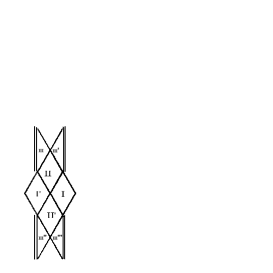
Figure 6: Penrose diagram for the $\cosh$ solution with $m=n=1$ and $\lambda_{+}=-2/p$ with $p$ odd; and for the $\sinh$ solution with $u_{0}>0$ and $\lambda_{+}=2/(p+1)$ ($m=n=1$) with $p$ odd or $\lambda_{+}=2/(n+1)$ ($m=1$) with $n$ odd or $\lambda_{+}=1$ with $m=n$ odd, or with $u_{0}<0$ ($b^{2}>0,m=n=1$) and $\lambda_{+}=-2/p$) with $p$ odd.

      In both subcases the geodesics can be continued until $x\rightarrow-\infty$ ($r=r_{-}$). In this limit, we obtain $H\sim x^{n+mp}\to\infty$ and $y\sim x^{-n-mp-1}\rightarrow 0$, corresponding to a singularity. In the first subcase (4.13), the maximally extended spacetime is represented by a diagram (Fig. 6) similar to that of Reissner-Nördstrom (but with signature ($+-++$)in region III) if $p$ is odd, or by the diagram of Fig. 7 (further discussed below) if $p$ is even. In the second subcase (4.15), the spacetime is represented by the diagram of Fig. 7 if $n$ is odd ($p$ even), or the diagram of Fig. 8 (with signature ($+-++$) in region II) if $n$ is even ($p$ odd).

   4. For $\lambda_{+}>0$, $H\to\infty$ and $y\to 0$ so that $x=-1$ corresponds to a singularity. As in case (2a), we find the Schwarzschild diagram (Fig. 1) for $n$ odd and the extreme Reissner-Nordstrom diagram (Fig. 2) for $n$ even.

Note that the global structure of the black hole spacetimes with a non-degenerate, or oddly degenerate, outer horizon $r=r_{+}$ (order $n$), followed by an evenly degenerate inner horizon $r=0$ (order $p$) hiding a spacelike singularity $r=r_{-}$ , cannot be represented by a two-dimensional Penrose diagram. The diagram of Fig. 7 represents faithfully the global topology of these spacetimes, at the price of representing the infinite sequence of bifurcate null asymptotically Minkowskian boundaries as dotted vertical (timelike) lines, each corresponding to the past and future null infinities of two contiguous regions I.

4.2 The linear solution

For the metric (3.25) with $m=n=1$, the geodesic equation (3.4) becomes

$$\frac{4b^{2}x_{1}^{2}\dot{x}^{2}}{(x-x_{1})^{4}}=E^{2}-cxe^{q_{1}x}\left[\epsilon+\frac{L^{2}c}{4b^{2}x_{1}}(x-x_{1})^{2}e^{q_{1}x}\right]\,,$$ (4.16)

and the conformal form of this metric is (4.2), with

$$dy=\pm\frac{2bx_{1}}{c}\frac{e^{-q_{1}x}}{x(x-x_{1})^{2}}dx\,.$$ (4.17)

As before, the limit $x\rightarrow x_{1}$ corresponds to the asymptotically Minkowskian region, and $x\rightarrow 0$ to the regular event horizon. The analysis of the limit $x\rightarrow-\infty$ depends on the sign of $q_{1}$.

1. For $q_{1}<0$ ($\eta_{2}=-1$), $y\rightarrow 0$, so that $x=-\infty$ corresponds to a singularity, and the Penrose diagram is that of Schwarzschild (Fig. 1).

2. For $q_{1}>0$ ($\eta_{2}=+1$), $y\rightarrow\pm\infty$, corresponding to a horizon. Near this horizon the geodesic equation (4.16) reads, in terms of the variable $z=-1/(x-x_{1})$ ($z\to 0$)

   $$4b^{2}x_{1}^{2}\dot{z}^{2}\simeq E^{2}+c^{\prime}z^{-1}e^{-q_{1}/z}\left[\epsilon+\frac{L^{2}c^{\prime}}{4b^{2}x_{1}}z^{-2}e^{-q_{1}/z}\right]$$ (4.18)

   ($c^{\prime}=ce^{q_{1}x_{1}}>0$). The effective potential goes to 0 for $z\to+0$, but goes to $+\infty$ for $z\to-0$ and $L^{2}>0$ with $\epsilon>0$ or $L^{2}>0$, so that radial timelike geodesics and all non-radial geodesics terminate due to an infinite potential barrier. So the apparent horizon $x\rightarrow-\infty$ is actually a null singularity. The corresponding Penrose diagram is represented by Fig. 4 (with in this case the signature (- + - -) in region II).

4.3 The phantom $\sinh$ solutions

As we have seen in Subsect. 3.3, there are three cases, according to the value of $u_{0}$.

1. For $u_{0}>0$, $J(u)$ is necessarily given by the first solution (2.23), and the metric can be written in the form (3.31), which is asymptotically Minkowskian in the limit $x\rightarrow x_{1}<1$. For $m$ and $n$ integer, the metric can be extended across the event horizon (of order $n$) at $x=0$. The next possible coordinate singularity is at $x=-1$, where the analysis can be carried over from the cosh case, provided the parity of $m$ is changed:

   1. $m$ odd. In this case, $x=-1$ is regular, and the geodesics extend until $x=-\infty$. The nature of this coordinate singularity depends on the value of $\lambda_{+}$.

      1. For $\lambda_{+}<0$, as in the cosh case, $x=-\infty$ is a singularity. The Penrose diagram is given by Fig. 1 for $n$ odd, and Fig. 2 for $n$ even.

      2. For a generic value of $\lambda_{+}>0$, $x=-\infty$ is a null singularity. The Penrose diagram is given by Fig. 3 for $n$ odd, and Fig. 4 for $n$ even.

      3. For $m=n=1,\lambda_{+}=2/(p+1)$ (the first solution of (4.7)-(4.8)), with $p$ positive integer, the metric (3.1) reads

         $$dS^{2}=f_{+}f_{-}^{p}dt^{2}-f_{+}^{-1}f_{-}^{-p}dr^{2}-r^{2}f_{-}^{-p+1}d\Omega^{2}\,.$$ (4.19)

         This metric has two regular horizons $r_{+}$ ($x=0$)and $r_{-}$ ($x=-\infty$) hiding the singularity $r=0$. For $p$ odd, the Penrose diagram is of the ”normal” Reissner-Nordström type, with signature ($+---$) in region III (Fig. 6). For $p$ even, the diagram is that of Fig. 7.

      4. For $m=p=1,\lambda_{+}=2/(n+1)$, the coordinate transformation $x=1/z<0$ leads to the metric

         $$dS^{2} = \frac{(-1)^{n+1}cz}{(1-z)^{n+1}}dt^{2}-\frac{(-1)^{n+1}4b^{2}z_{1}(1-z)^{n+1}}{c(z-z_{1})^{2}}\times$$ (4.20)

         $$\times\bigg{[}\frac{z_{1}dx^{2}}{z(z-z_{1})^{2}}+d\Omega^{2}\bigg{]}\,,$$

         ($z_{1}=1/x_{1}$). This can be continued across the horizon $z=0$ until the singularity $z=1$. The spacetime is represented by the normal Reissner-Nordström diagram (Fig. 6) if $n$ is odd, and by Fig. 8 if $n$ is even.

      5. For $m=n=p$ ($\lambda_{+}=1$, Einstein-Maxwell-anti-scalar case), the metric

         $$dS^{2}=\frac{cx^{n}}{(1-x^{n})^{2}}dt^{2}-\frac{4b^{2}x_{1}x^{1-n}(1-x^{n})^{2}}{c(x-x_{1})^{2}}\bigg{[}\frac{x_{1}dx^{2}}{x(x-x_{1})^{2}}+d\Omega^{2}\bigg{]}\,,$$ (4.21)

         is form-invariant under the combined inversion $x\to z=1/x$, $x_{1}\to z_{1}=1/x_{1}$. The difference with the Einstein-Maxwell-scalar case is that now to $x_{1}<1$ corresponds $z_{1}>1$. The coordinate $z$ increases from $z=-\infty$ (event horizon) through $z=0$ (second horizon) to the singularity $z=1$. As $n$ is odd, the Penrose diagram is again of the normal Reissner-Nordström type (Fig. 6).

   2. $m$ even. In this case, there is a coordinate singularity at $x=-1$. Putting $x=-1+z$, we obtain for the geodesic equation near $z=0$ the form (4.11). Therefore the analysis proceeds as in case 2 of Subsect. 4.1, except for the case $\lambda_{+}=-2/p$ which does not occur in the present case because $m$ is even. It follows that $x=-1$ is in all cases a true singularity, which is null for $-2\leq\lambda_{+}<0$.

2. For $u_{0}=0$ (again with only the first solution (2.23) for $J(u)$), the only difference with the preceding analysis is that the metric (3.33) is non-asymptotically flat (NAF) for $x\to x_{1}$. The geodesic equation for the asymptotic metric (3.34) is:

   $$\dot{r}^{2}\sim E^{2}-\bigg{(}\frac{r}{r_{+}}\bigg{)}^{2/\lambda_{+}}\bigg{[}\epsilon+\bigg{(}\frac{r}{r_{+}}\bigg{)}^{2/\lambda_{+}}\frac{L^{2}}{r^{2}}\bigg{]}\,.$$ (4.22)

   For $\lambda_{+}<0$, the effective potential goes to zero for $r\to\infty$, which is at infinite geodesic distance. The conformal radial coordinate $y$, given asymptotically by $dy\sim(r/r_{+})^{-2/\lambda_{+}}dr$ also goes to infinity, so that the conformal metric is asymptotically Minkowskian. The extension across the horizon $x=0$ ($r=r_{+}$) proceeds as in the case $u_{0}>0$ and leads to the same Penrose diagrams, i.e. Fig. 1 for $n$ odd and $m$ odd or $m$ even with $\lambda_{+}<-2$, Fig. 2 for $n$ even and $m$ odd or $m$ even with $\lambda_{+}<-2$, Fig. 3 for $n$ odd and $m$ even with $-2\leq\lambda_{+}<0$, and Fig. 4 for $n$ even and $m$ even with $-2\leq\lambda_{+}<0$.

   For $0<\lambda_{+}<1$, equation (4.22) leads asymptotically to $s\sim r^{1-1/\lambda_{+}}$, so that geodesics terminate at the conformally timelike singularity $r\to\infty$. These solutions do not correspond to black holes. However, for $\lambda_{+}=1$ ($m=n$), asymptotically $s\sim\ln{r}$, and geodesics are complete, but spatial infinity is still conformally timelike. The extension of the metric (4.21) with $x_{1}=1$ proceeds similarly to the case $u>u_{0}$. For $m=n$ odd, this metric is regular at $x=-1$ and form-invariant under the combined inversion $x\to z=1/x$, leading after extension through the two horizons $x=0$ and $z=0$ to a geodesically complete spacetime (Fig. 9). For $m=n$ even, the spacetime has a single horizon $x=0$ and a conformally timelike singularity $x=-1$ (Fig. 10).

3. For $u_{0}<0$, we have seen that the event horizon at $u=u_{0}$ is regular (of order $p$) if $\lambda_{+}=-2/p$ (for any $m$ and $n$ real). The properties of the metric inside the event horizon ($u<u_{0}$) depend on the solution (2.23) for $J(u)$.

   1. First solution (2.23). The form of the metric (3.31) shows that $x=0$ ($u\to-\infty$) is a horizon, which is regular if $m$ and $n$ are positive integers. Because $\lambda_{+}=-2/p$, these must satisfy Eq. (4.12). So there are three possibilities:

      1. For $m$ and $n$ generics, $u=-\infty$ is a null singularity. The Penrose diagram is given by Fig. 3 for $p$ odd, and Fig. 4 for $p$ even.

      2. For $m=n=1$, geodesics terminate at the singularity $x\rightarrow-\infty$. The Penrose diagram is given by Fig. 6 for $p$ odd, and by Fig. 8 for $p$ even.

      3. For $m=2n+1,p=n-1$, the singularity is again at $x\rightarrow-\infty$. The Penrose diagram is now given by Fig. 7 for $p$ odd, and by Fig. 8 for $p$ even.

   2. Second solution (2.23). The metric is (3.36) with $b=0$ and $\varphi_{1}=\pm a$ (which follows from (2.33)), leading to

      $$h(u)=e^{\mp a\lambda u}\sinh a(u-u_{0})\,.$$ (4.23)

      The associated geodesic equation is

      $$\dot{r}^{2}=E^{2}-ch^{p}[\epsilon-L^{2}ch^{p}/r^{2}]\,,$$ (4.24)

      with $r=-1/u>0$. Near the singularity $r=0$ ($u\to-\infty$), $h(r)\simeq e^{(1\pm\lambda)a/r}/2$, so that the analysis follows closely that made in Subsect. 4.2. Taking into account $\lambda^{2}>1$, there are two possibilities:

      1. If $\pm\lambda>1$, $h(r)$ diverges, leading to a space-like singularity if $p$ is odd (Fig. 1), or a time-like singularity if $p$ is even (Fig. 2).

      2. If $\pm\lambda<-1$, $h(r)$ vanishes, signalling a horizon. However the effective potential in (4.24) diverges for $r\to-0$ ($h(r)\simeq e^{(1\mp\lambda)a/|r|}/2$), so $r=0$ is actually a null singularity. The Penrose diagram is given by Fig. 3 if $p$ is odd, and Fig. 4 if $p$ is even.

   3. Third solution (2.23). In (3.36), $e^{2J}=\bar{b}^{2}/\sin^{2}\bar{b}u$. So the metric has apparent singularities at $u=u_{s_{k}}\equiv k\pi/\bar{b}$ ($k$ integer). Putting $u=u_{s_{k}}+z$, the metric near $z=0$ goes to the asymptotically flat form

      $$dS^{2}=c^{\prime}dt^{2}-c^{{}^{\prime}-1}(z^{-4}dz^{2}+z^{-2}d\Omega^{2})\,,$$ (4.25)

      with $c^{\prime}=ch^{p}(u_{s})$. So, in a generic solution sector $u_{s_{k}}<u<u_{s_{k+1}}$ which does not contain $u_{0}$, we have a geodesically complete, horizonless spacetime with two asymptotic regions — a Lorentzian wormhole [23] generalizing the $\lambda=0$ Bronnikov wormhole of Einstein-Maxwell-anti-scalar theory [15]. In the solution sector which contains $u_{0}$, the spacetime is still geodesically complete with a horizon of order $p$. The corresponding Penrose diagrams are given in Fig. 11 for $p$ odd, and Fig. 12 for $p$ even.

4.4 The $a=0$ solutions

We have seen in Subsect. 3.4 that there are two regular black hole cases:

1. For $u_{0}\geq 0$, $a=b=0$, the metric is given by (3.39) with $\lambda_{+}=2/(p+1)$. This has a horizon of order (p+1) at $r=0$ ($u\to-\infty$), and a singularity at $r=-1/u_{0}$. Therefore, for $u_{0}>0$ the Penrose diagram is given by Fig. 1 if $p$ is even, and Fig. 2 if $p$ is odd.

   For $u_{0}=0$, (3.39) is replaced by the non-asymptotically flat metric

   $$dS^{2}=\left(\frac{r}{r_{+}}\right)^{p+1}dt^{2}-\left(\frac{r}{r_{+}}\right)^{-(p+1)}(dr^{2}+r^{2}d\Omega^{2})\,.$$ (4.26)

   The two-dimensional reduced metric is similar to that of the ’first-class’ black holes of [16]. Spacelike infinity $r\to\infty$ is conformally timelike. For $p$ even, geodesics cross the odd horizon $r=0$ and terminate at the conformally spacelike singularity $r\to-\infty$ (Fig 13). For $p$ odd, $r\to-r$ is an isometry of the metric (4.26). The Penrose diagram of these geodesically complete spacetimes is given in Fig. 14.

2. For $u_{0}<0$, the metric is (3.36) with $h(u)$ given by (3.41). This has a horizon of order $p$ at $u=u_{0}$ and a coordinate singularity at $u\to-\infty$. If $b^{2}>0$ ($\varphi_{1}\neq 0$), the metric written in terms of the coordinate $x$ contains again a non-analytic logarithm, so that $u\to-\infty$ ($x=0$) is a true singularity. If $b^{2}=0$, the metric reduces to (3.42), which is clearly singular for $u\to-\infty$ ($r=0$). In both cases, the Penrose diagram is given by Fig. 1 if $p$ is odd, and Fig. 2 if $p$ is even.

4.5 The $\sin$ solution

As seen in subsection (3.5), for this case the only possibility leading to black holes occurs for the first solution (2.23) for $J(u)$, and is of the form (3.36) with $h(u)$ given by (3.44). This can be rewritten as

$$h(u)=e^{-\lambda\varphi_{1}u}\sin\bar{a}(u-u_{s})\,,$$ (4.27)

for $u_{s}<u<0$, where $u_{s}=u_{0}+k\pi/\bar{a}$, with $-\pi/\bar{a}<u_{s}<0$. The asymptotically Minkowskian (for $u\to 0$) spacetime therefore presents an infinite series of regular horizons $u=u_{s}$, $u=u_{s}-\pi/\bar{a}$, $u=u_{s}-2\pi/\bar{a}$, $\cdots$, all of order $p$, separating successive regions $I$, $II$, $III$, $\cdots$ which are all different (because of the non-periodic functions $e^{2J(u)}$ and $e^{-\lambda\varphi_{1}u}$). This spacetime is geodesically complete. For $p$ even, the successive regions all have the same light-cone orientation. The corresponding Penrose diagram is represented in Fig. 15. On the other hand, for $p$ odd, the light-cone orientations alternate between successive regions, so that geodesics can wind around indefinitely. It is not possible to draw a flat Penrose diagram for this case.

Figure 1: Penrose diagram for the $\cosh$ solution with $n$ odd and $m$ even ($\lambda_{+}<0$) or $m$ odd ($\lambda_{+}<-2$ or $\lambda_{+}>0$); for the linear solution with $n=m=1$ and $q_{1}<0$; for the $\sinh$ solution with $n$ odd and $m$ odd ($u_{0}\geq 0,\lambda_{+}<0$) or $m$ even ($u_{0}\geq 0,\lambda_{+}<-2$ or $u_{0}>0,\lambda_{+}>0$), or with $b=0$ ($u_{0}<0,\lambda_{+}=-2/p,\pm\lambda>1$) and $p$ odd; and for the $a=0$ solution with $b=0$ ($u_{0}>0,\lambda_{+}=2/(p+1)$) and $p$ even or with $b^{2}\geq 0$ ($u_{0}<0,\lambda_{+}=-2/p$) and $p$ odd. The central singularity is represented by a double line.

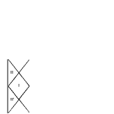
Figure 2: Penrose diagram for the $\cosh$ solution with $n$ even and $m$ even ($\lambda_{+}<0$) or $m$ odd ($\lambda_{+}<-2$ or $\lambda_{+}>0$); for the $\sinh$ solution with $n$ even and $m$ odd ($u_{0}\geq 0,\lambda_{+}<0$) or $m$ even ($u_{0}\geq 0,\lambda_{+}<-2$ or $u_{0}>0,\lambda_{+}>0$), or with $b=0$ ($u_{0}<0,\lambda_{+}=-2/p,\pm\lambda>1$) and $p$ even; and for the $a=0$ solution with $b=0$ ($u_{0}>0,\lambda_{+}=2/(p+1)$) and $p$ odd or with $b^{2}\geq 0$ ($u_{0}<0,\lambda_{+}=-2/p$) and $p$ even.

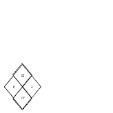
Figure 3: Penrose diagram for the cosh solution with $n$ odd and $m$ even ($\lambda_{+}>0$) or $m$ odd ($-2\leq\lambda_{+}<0$); and for the $\sinh$ solution with $n$ odd and $m$ odd ($u_{0}>0,\lambda_{+}>0$) or $m$ even ($u_{0}\geq 0,-2<\lambda_{+}<0$), or $u_{0}<0$ and $\lambda_{+}=-2/p$ with $p$ odd ($b^{2}>0$ or $b=0$ and $\pm\lambda<-1$).

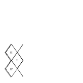
Figure 4: Penrose diagram for the cosh solution with $n$ even and $m$ even ($\lambda_{+}>0$) or $m$ odd ($-2\leq\lambda_{+}<0$); for the linear solution with $n=m=1$ and $q_{1}>0$; and for the $\sinh$ solution with $n$ even and $m$ odd ($u_{0}>0,\lambda_{+}>0$) or $m$ even ($u_{0}\geq 0,-2<\lambda_{+}<0$), or $u_{0}<0$ and $\lambda_{+}=-2/p$ with $p$ even ($b^{2}>0$ or $b=0$ and $\pm\lambda<-1$).

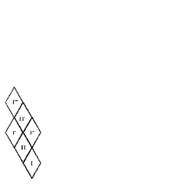
Figure 5: Penrose diagram for the $\cosh$ solution with $\lambda_{+}=1$, $m=n$ even

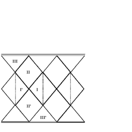
Figure 7: Penrose diagram for the $\cosh$ solution with $\lambda_{+}=-2/p$ and $p$ even ($m=n=1$ or $m=2n+1,p=n-1$); and for the $\sinh$ solution with $u_{0}>0,\lambda_{+}=2/(p+1)$ and $p$ even ($m=n=1$), or with $u_{0}<0,\lambda_{+}=-2/p$ ($m=2n+1,p=n-1$ odd).

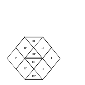
Figure 8: Penrose diagram for the $\cosh$ solution with $\lambda_{+}=-2/p$ and $p$ odd ($m=2n+1,p=n-1$); and for the $\sinh$ solution with $u_{0}>0,\lambda_{+}=2/(n+1)$ and $n$ even ($m=1$), or with $u_{0}<0,\lambda_{+}=-2/p$ and $p$ even ($m=n=1$ or $m=2n+1,p=n-1$).

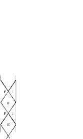
Figure 9: Penrose diagram for the $\sinh$ solution with $u_{0}=0,\lambda_{+}=1,m=n$ odd.

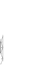
Figure 10: Penrose diagram for the $\sinh$ solution with $u_{0}=0,\lambda_{+}=1,m=n$ even.

Figure 11: Penrose diagram for the $\sinh$ solution with $u_{0}<0$ ($b^{2}<0$) and $\lambda_{+}=-2/p$, $p$ odd.

Figure 12: Penrose diagram for the $\sinh$ solution with $u_{0}<0$ ($b^{2}<0$) and $\lambda_{+}=-2/p$, $p$ even.

Figure 13: Penrose diagram for the $a=0$ solution ($b=0,u_{0}=0,\lambda_{+}=-2/(p+1)$) with $p$ even.

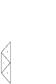
Figure 14: Penrose diagram for the $a=0$ solution ($b=0,u_{0}=0,\lambda_{+}=-2/(p+1)$) with $p$ odd.

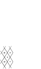
Figure 15: Penrose diagram for the $\sin$ solution with $\lambda_{+}=-2/p$, $p$ even.

5 Conclusions

We have determined in this paper the general static, spherically symmetric solutions for the four-dimensional EMD theory when the scalar field and/or the electromagnetic field are allowed to violate the null energy condition. The general solution given by (2.22) contains nine classes of asymptotically flat phantom black holes: the “cosh” solution, the “linear” solution, the “sinh” solution with $u_{0}>0$, the “sinh” solution with $u_{0}<0$ (three classes), the “a=0” solution with $u_{0}>0$, the “a=0” solution with $u_{0}<0$, and the “sin” solution. There are also two classes of non-asymptotically flat phantom black holes, corresponding to the sinh and the a=0 solutions with $u_{0}=0$.

The event horizon of these black holes can be either non-degenerate or degenerate. Besides the previously known phantom black holes with a single event horizon [9, 20], which occur for generic values of the dilatonic coupling constant, we have obtained for certain discrete values of this coupling constant new phantom black holes with a single event horizon, as well as cold black holes, with a degenerate event horizon. A noteworthy consequence of the violation of the null energy condition is that, for the special case of a vanishing dilaton coupling constant, there is an infinite sequence of black holes with multiple event horizons, of the cosh type in the Einstein-anti-Maxwell-anti-scalar case, and of the sinh type in the Einstein-Maxwell-anti-scalar case.

We have paid special attention to the study of the causal structures of these phantom black holes. In total, we have found $16$ different types of causal structures. Many cases lead to Penrose diagrams similar to those of the “classical” Schwarzschild, Reissner-Nordström, or extreme Reissner-Nordström black holes. However, there are new causal structures. Some of them differ from the preceding by the fact that the central spacelike or timelike singularity is replaced by a null singularity (Figs. 3, 4), or that null infinity is replaced by timelike infinity (Figs. 10, 13). A number of these spacetimes are geodesically complete with one degenerate horizon (Figs. 11, 12, 14) or two equally degenerate horizons (Figs. 5, 9). We also found more complex structures. The maximal analytic extension of a black hole with an event horizon of even order and an inner horizon of odd order has a tower of spacelike singularities (Fig. 8). The opposite case of an odd event horizon and an even inner horizon cannot be represented by a two-dimensional conformal diagram, it is possible to represent only the global spacetime topology (Fig. 7). The most exotic, geodesically complete, spacetimes have an infinite sequence of equally degenerate horizons separating successive non-isometrical regions; this structure is represented in Fig. 15 for even horizons, the case of oddly-degenerate horizons does not admit a two-dimensional representation.

There is a discussion in the literature whether phantom black holes could be formed by gravitational collapse of a phantom fluid [20, 24]. In any case, these phantom black holes could perhaps also be created by another mechanism, such as a tunneling quantum process. Of course, since for a phantom fluid all energy conditions are violated, the stability of the configurations described above remains another important question. The present work should also be complemented by the construction of rotating phantom black holes, and the analysis of the solutions corresponding to wormholes, which we mentioned only briefly at the end of Subsect. 4.3. We hope to address these questions in the future.

Acknowledgements: J.C. Fabris and M.E.R. thank CNPq (Brazil), FAPES (Brazil) and the French-Brazilian scientific cooperation CAPES/COFECUB (project number 506/05) for partial financial support. They also thank the LAPTH (Annecy-le-Vieux, France), for hospitality during the elaboration of this work.

References

- [1] G.W. Gibbons and K. Maeda, Nucl. Phys. B 298, 741 (1988).
- [2] D. Garfinkle , G.T. Horowitz and A. Strominger, Phys. Rev. D 43, 3140 (1991).
- [3] K.C.K. Chan, J.H. Horne and R.B. Mann, Nucl. Phys. B 447, 441 (1995).
- [4] G. Clément, C. Leygnac and D. Gal’tsov, Phys. Rev. D 67, 024012 (2003).
- [5] G. Clément, C. Leygnac, Phys. Rev. D 70, 084018 (2004).
- [6] G. Clément, J.C. Fabris and G.T. Marques, Phys. Lett. B 651, 54 (2007).
- [7] C. Grojean, F. Quevedo, G. Tasinato and I. Zavala, JHEP 0108, 005 (2001).
- [8] G. Clément, C. Leygnac and D. Gal’tsov, Phys. Rev. D 71, 084014 (2005).
- [9] G. W. Gibbons and D. A. Rasheed, Nucl. Phys. B 476, 515 (1996).
- [10] M. Gasperini, F. Piazza and G. Veneziano, Phys. Rev. D 65, 023508 (2002).
- [11] F. Piazza and S. Tsujikawa, JCAP 0407, 004 (2004).
- [12] S. Hannestad, Int. J. Mod. Phys. A 21, 1938 (2006).
- [13] J. Dunkley at. al, Five years Wilkinson Microwave Anisotropy Probe (WMAP) observations: likelihood and parameters from the WMAP data, arXiv: 0803.0586.
- [14] H.G. Ellis, Journ. Math. Phys. 14, 104 (1973).
- [15] K. Bronnikov, Acta Phys. Pol. B 4, 251 (1973).
- [16] G. Clément and A. Fabbri, Class. Quantum Grav. 16, 323 (1999).
- [17] K.A. Bronnikov, M.S. Chernokova, J.C. Fabris, N. Pinto-Neto and M.E. Rodrigues, Int. J. Mod. Phys. D 17, 25 (2008).
- [18] K.A. Bronnikov, G. Clément, C.P. Constantinidis and J.C. Fabris, Phys. Lett. A 243, 121 (1998); Grav.&Cosm. 4, 128 (1998).
- [19] K.A. Bronnikov, C.P. Constantinidis, R.L. Evangelista and J.C. Fabris, Int. J. Mod. Phys. D 8, 481 (1999).
- [20] C.J. Gao and S.N. Zhang, Phantom black holes, hep-th/0604114.
- [21] K.A. Bronnikov and J.C. Fabris, Phys. Rev. Lett. 96, 251101 (2006).
- [22] D. Gal’tsov, J.P.S. Lemos and G. Clément, Phys. Rev. D 70, 024011 (2004).
- [23] M.S. Morris and K.S. Thorne, Am. J. Phys. 56, 395 (1988).
- [24] R.-G. Cai and A. Wang, Phys. Rev. D 73, 063005 (2006).