Generalized Voronoi Tessellation as a Model of Two-dimensional Cell Tissue Dynamics

Abstract

Voronoi tessellations have been used to model the geometric arrangement of cells in morphogenetic or cancerous tissues, however so far only with flat hypersurfaces as cell-cell contact borders. In order to reproduce the experimentally observed piecewise spherical boundary shapes, we develop a consistent theoretical framework of multiplicatively weighted distance functions, defining generalized finite Voronoi neighborhoods around cell bodies of varying radius, which serve as heterogeneous generators of the resulting model tissue. The interactions between cells are represented by adhesive and repelling force densities on the cell contact borders. In addition, protrusive locomotion forces are implemented along the cell boundaries at the tissue margin, and stochastic perturbations allow for non-deterministic motility effects. Simulations of the emerging system of stochastic differential equations for position and velocity of cell centers show the feasibility of this Voronoi method generating realistic cell shapes. In the limiting case of a single cell pair in brief contact, the dynamical nonlinear Ornstein-Uhlenbeck process is analytically investigated. In general, topologically distinct tissue conformations are observed, exhibiting stability on different time scales, and tissue coherence is quantified by suitable characteristics. Finally, an argument is derived pointing to a tradeoff in natural tissues between cell size heterogeneity and the extension of cellular lamellae.

1 Introduction

A Voronoi tessellation is a partition of space according to certain neighborhood relations of a given set of generators (points) in this space. Initially proposed by Dirichlet for special cases [16], the method was established by Voronoi more than 100 years ago [45]. The geometric dual of the Voronoi tessellation was proposed by Delaunay in 1934 — and therefore is called Delaunay triangulation. It connects those points of a Voronoi tessellation that share a common border. Since the latter can be directly constructed out of the former, both terms are sometimes used equivalently. In the following years, the method was rediscovered throughout other fields, which accounts for many other names designating the very concept, such as Thiessen polygons [43] in meteorology or Wigner-Seitz cells [48] and Brillouin zones [13] in solid state physics. With the technological and scientific advance, the method became feasible in computational geometry [39], and since then has widely evolved, cf. [9, 8], making it appealing for biological applications.

In particular, Voronoi tessellations have been applied to represent various aggregates of cells and swarming animals. Initially, Honda proposed the method in two spatial dimensions [24]. The first applications to biological tissue were cell sorting simulations, however starting from artificially shaped quadratic cells [41]. Then, morphogenesis and its underlying intercellular mechanisms were studied starting from a pure Delaunay mesh and simulating vertex dynamics [47, 46], yet without using Voronoi tessellations explicitly. In contrast, by applying transformation rules like mitosis combined with Monte-Carlo dynamics, evolving multicellular tissue was represented by Voronoi tessellations [18]. In particular, growth instabilities, blastula formation and gastrulation could be conceived within this framework [17]. Similar effects were reproduced by using vertex dynamics [14]. Moreover, cell organization in the intestinal crypt was modelled using spring forces and restricting the motion to a cylindrical surface [32]. An application to bird swarming together with the proposal of a continuum formulation was given in [3]. Finally, the influence of shear stress on the evolution of two-dimensional tissues was studied [15].

Only quite recently Voronoi tessellations have been extended to be used as a model for three dimensional tissue, again using vertex dynamics [25]. Other authors use optimized kinetic algorithms [36, 11] to employ generalized Voronoi tessellations (discussed as difference method in this article), with cell-cell and cell-matrix adhesion [37]. Marginal cells have been closed by prescribing a maximal cell radius, enabling the study of the growth dynamics of epithelial cell populations [21]. So far, however, the cell-cell boundaries were exclusively represented by flat hypersurfaces.

In contrast, when observing two-dimensional monolayers of keratinocytes, for example cf. [49, 31, 44], the cell-cell contact borders visible from staining cadherin-complexes frequently appear as circular arcs, whose shape and length seems to be determined by the constellation and size distribution of neighboring cells. Moreover, the forces between such cells are influenced by filament networks or bundles meeting at the cell-cell junctions and eventually balanced by elastic counterforces [1, 4, 29, 40]. Therefore, a geometrical and dynamical modeling framework is required that reproduces the observed cell shapes and simultaneously allows for quantifying the cell-cell interaction forces as well as the active locomotion forces appearing at the free cell boundaries. Here we present a simple and effective solution of this task by using a suitably weighted Voronoi tessellation.

This article is organized as follows: In section 2 Voronoi tessellations are introduced in a general manner. Next, two types of weighted square distance functions are introduced, using the method of difference and quotient, respectively, and their particular consequences for cell tissue modeling are investigated. Inspired by the intricate interplay between cytoskeletal filament bundles and cadherin-catenin cohesion or integrin adhesion sites, the forces on the intercellular and exterior cell borders are proposed in section 3 after discussing the emergence of cell shape within our model. Then the dynamics of a whole cell aggregate is defined, directly leading to analytical results on cell pair contacts in section 4. After simulation studies of meta-stable states during tissue equilibration and robustness of tissue formation under the influence of various model parameters in section 5 we conclude with a discussion of our results in section 6.

2 Generalized Voronoi tessellations

Let $\{g_{i}:i=1\dots N\}$ denote a finite set of $N$ generators or points $\mathbf{x}_{i}$ in Euclidean, $n$-dimensional space $\mathbb{R}^{n}$.

Definition 1.

The Voronoi cell of a generator $g_{i}=\mathbf{x}_{i}$ is defined as

$$\mathcal{V}_{i}=\left\{\mathbf{x}\in\mathbb{R}^{n}:\mathcal{P}_{i}(\mathbf{x})<\mathcal{P}_{j}(\mathbf{x})\quad\forall j\neq i\right\},$$ (1)

where $\mathcal{P}_{i}$ $(i=1\dots N)$ is a given set of continuous, generalized square distance functions on $\mathbb{R}^{n}$ with the property that $\forall i:\;\mathbf{x}_{i}\in\mathcal{V}_{i}$.

Thus, $\mathcal{V}_{i}$ represents an open neighborhood of $\mathbf{x}_{i}$, containing all points $\mathbf{x}$ that are $\mathcal{P}$-closer to $\mathbf{x}_{i}$ than to any other $\mathbf{x}_{j}$.

Definition 2.

The contact border between two points $\mathbf{x}_{i}$ and $\mathbf{x}_{j}$ is defined as the intersection of the closures of $\mathcal{V}_{i},\mathcal{V}_{j}$:

$$\Gamma_{ij}=\overline{\mathcal{V}}_{i}\cap\overline{\mathcal{V}}_{j}\quad\text{with}\;\;i\neq j.$$ (2)

The total boundary of the Voronoi neighborhood around $\mathbf{x}_{i}$ then is

$$\partial\mathcal{V}_{i}=\bigcup_{j\neq i}\Gamma_{ij}\;.$$

The contact border $\Gamma_{ij}$ therefore is the set of all points $\mathcal{P}$-equidistant from $\mathbf{x}_{i}$ and $\mathbf{x}_{j}$, namely

$$\Gamma_{ij}=\left\{\mathbf{x}\in\mathbb{R}^{n}:\mathcal{P}_{i}(\mathbf{x})=\mathcal{P}_{j}(\mathbf{x})\leq\mathcal{P}_{k}(\mathbf{x})\;\forall k\neq i,j\right\}.$$ (3)

The Voronoi tessellation in general form is then given by $\{\mathcal{V}_{i},\Gamma_{ij};\;i,j=1,\dots,N\}$ and covers the whole space, where so-called marginal neighborhoods $\mathcal{V}_{i}$ extend to infinity. Depending on the particular choice of the generalized square distance functions, $\Gamma_{ij}$ can take various shapes. In the standard Euclidean case, $\mathcal{P}_{i}(\mathbf{x})=|\mathbf{x}-\mathbf{x}_{i}|^{2}$, the contact border $\Gamma_{ij}$ is the perpendicular bisector of the line segment from $\mathbf{x}_{i}$ to $\mathbf{x}_{j}$, an $(n-1)$-plane. Then $\mathcal{V}_{i}$ is bounded by a convex, not necessarily finite polytope and is called the (classical) Voronoi neighborhood [45] or Dirichlet domain [16].

The modeling aim here is to represent biological eukaryotic cells in connected $3$-dimensional tissues or confluent $2$-dimensional cell monolayers as Voronoi neighborhoods $\mathcal{V}_{i}$, as in the $2$-dimensional pictures in figure 1.

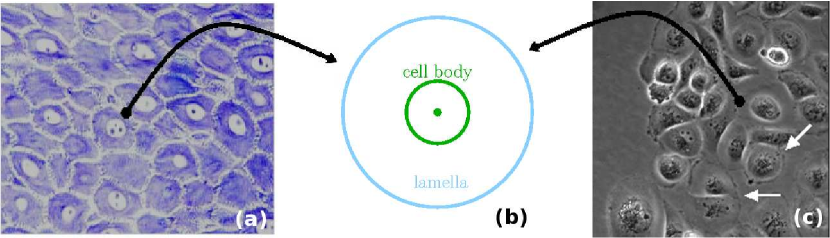
Figure 1: (a) Micrograph of human keratinocytes in a section of stratum spinosum in vivo (reproduced from [49]), and (c) phase contrast microscopic photograph of human keratinocytes in-vitro (by courtesy of Institute of Cell Biology, Bonn University). Image (c) is extracted from the supplementary movie mov0.avi of the dynamics at the edge of an almost confluent monolayer in a wound scratch assay. White arrows in (c) indicate a round cell (upper) and a cell pair competing for its influence region (lower). According to these observations, tissue cells in a two-dimensional geometry are modelled as Voronoi neighborhoods $\mathcal{V}_{i}$ containing the ball shaped cell bodies $\mathcal{B}_{r_{i}}(\mathbf{x}_{i})$ surrounded by a so-called lamella (b).

In a minimal approach we define the points $\mathbf{x}_{i}$ as centers of the visible, mostly ball-shaped cell bodies, containing the cell nuclei plus other cell organelles such as mitochondria or the Golgi apparatus. By attributing a finite radius $r_{i}>0$ to each $\mathbf{x}_{i}$, the Voronoi concept is extended to generators $g_{i}=\mathcal{B}_{r_{i}}(\mathbf{x}_{i})$ of positive finite volume, being a suitable representation of cell bodies. Since these are rather solid in comparison to the rest of the cell, it is assumed that the $\mathcal{B}_{r_{i}}(\mathbf{x}_{i})$ do not overlap. Then $\mathcal{V}_{i}\setminus\mathcal{B}_{r_{i}}(\mathbf{x}_{i})$ represents the protoplasmic region of the cell $i$, which for $n=2$ appears as a flat lamella in light microscopy. Clearly, the natural condition $\overline{\mathcal{B}_{r_{i}}(\mathbf{x}_{i})}\subset\mathcal{V}_{i}$ requires that

$$\forall\mathbf{x}\in\overline{\mathcal{B}_{r_{i}}(\mathbf{x}_{i})}\quad\forall j\neq i:\quad\mathcal{P}_{j}(\mathbf{x})>\mathcal{P}_{i}(\mathbf{x}).$$ (4)

It shall be seen later, that this condition is fulfilled for the chosen generalized square distance functions.

Furthermore, certain weights $w_{i}\in\mathbb{R}^{+}$, on which the square distance function $\mathcal{P}_{i}$ may depend, are assigned to each cell $i$. These weights $w_{i}=w(r_{i})$ are assumed to be strictly monotonically increasing functions of the cell body radius $r_{i}$, with the intended effect that stronger weights induce larger cell sizes, by shifting the Voronoi contact borders outwards. Importantly, different choices of how $\mathcal{P}_{i}$ depends on $w_{i}$ could lead to different cell shapes. Out of many possible generalizations of Voronoi tessellations (for a review see [8]), we only discuss two straight-forward ways here, which are determined by the set of all cell center positions, body radii and weights $\{g_{i}=(\mathcal{B}_{r_{i}}(\mathbf{x}_{i}),w_{i})\}$.

2.1 Difference method

The partition of space into cells is obtained by a Voronoi tessellation using the Euclidean square distance function with subtracted weights

$$\mathcal{P}_{i}(\mathbf{x})=(\mathbf{x}-\mathbf{x}_{i})^{2}-w_{i}^{2},$$ (5)

which has previously been used in [24, 25] without and in [37, 10] with weights $w_{i}$.

For the following we denote $\mathbf{x}_{ij}=(\mathbf{x}_{i}+\mathbf{x}_{j})/2$ the cell pair mid-point, $d_{ij}=|\mathbf{x}_{i}-\mathbf{x}_{j}|$ the Euclidean cell center distance, and $\hat{\mathbf{d}}_{ij}=(\mathbf{x}_{i}-\mathbf{x}_{j})/d_{ij}$ the unit vector of the oriented axis connecting the two cell centers. Thus, from equation (3) the condition for a point $\mathbf{x}$ to be located on the contact border $\Gamma_{ij}$ reads as

$$\bigl{(}\mathbf{x}-\mathbf{x}_{ij}\bigr{)}\cdot\hat{\mathbf{d}}_{ij}=-\frac{w_{i}^{2}-w_{j}^{2}}{2d_{ij}},$$ (6)

being equivalent to a linear hyper-plane equation. As for the classical Voronoi partition, the contact $(n-1)$-plane between two neighboring cells $i,j$ is perpendicular to the vector connecting the cell centers. However, now the position of the contact border plane along the connecting vector, and thereby the sizes of the Voronoi cells, depend on the weights.

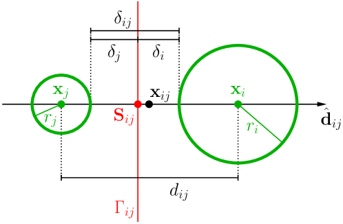
Figure 2: Geometry of a cell pair and its border using the difference method. There is a distinct direction $\hat{\mathbf{d}}_{ij}$ given by the axis line connecting $\mathbf{x}_{j}$ and $\mathbf{x}_{i}$. The circular cell bodies around $\mathbf{x}_{i},\mathbf{x}_{j}$ and their radii $r_{i},r_{j}$ are indicated by green lines, the contact hyperplane $\Gamma_{ij}$ by a red one. Other quantities are explained in the text.

In figure 2 the geometry of a cell pair with its separating border is illustrated.

In order for a distance function to yield a partition describing an aggregate of biological cells in living tissue, the border $\Gamma_{ij}$ has to be located between the surfaces of the non-overlapping cell bodies. With the corresponding distances as denoted in figure 2, this is equivalent to

$$\delta_{i}>0\quad\wedge\quad\delta_{j}>0.$$ (7)

These constraints have consequences for possible choices of the weights:

Lemma 1.

Let $\{\mathcal{V}_{i},\Gamma_{ij}\}$ be a Voronoi tessellation of non-overlapping generators $\{g_{i}=(\mathcal{B}_{r_{i}}(\mathbf{x}_{i}),w_{i})\}$ constructed from $\mathcal{P}_{i}$ according to the difference method in definition (5) with positive weights $w_{i}$. Then the inequalities (7) are satisfied for all cell pairs $i\neq j$ with arbitrarily small but positive cell body distance $\delta_{ij}=\delta_{i}+\delta_{j}$, if and only if

$$\forall i:\quad w_{i}=r_{i}.$$ (8)

Proof.

: The contact border equation $\mathcal{P}_{i}=\mathcal{P}_{j}$ evaluated at the intersection point $\mathbf{x}=\mathbf{S}_{ij}$, see figure 2, yields $(r_{i}+\delta_{i})^{2}-w_{i}^{2}=(r_{j}+\delta_{j})^{2}-w_{j}$. Together with $\delta_{i}+\delta_{j}=\delta_{ij}$ we obtain the representation

$$\delta_{i}=\frac{\delta_{ij}(\delta_{ij}+2r_{j})+(w_{i}^{2}-w_{j}^{2})-(r_{i}^{2}-r_{j}^{2})}{2(r_{i}+r_{j}+\delta_{ij})}>0.$$ (9)

Since $\delta_{ij}>0$ can be arbitrarily small for fixed $r_{i},r_{j}$ and $w_{i},w_{j}$, the condition $\delta_{i}>0$ implies $w_{i}^{2}-r_{i}^{2}\geq w_{j}^{2}-r_{j}^{2}$. By exchanging $i$ and $j$, the second condition $\delta_{j}>0$ enforces the equality and the existence of a joint constant $C$ with

$$w_{k}^{2}=r_{k}^{2}+C\quad\text{for}\quad k=i,j.$$

Since the definition 1 of a Voronoi cell is independent of such an additive constant in equation (5), we can set $C=0$ and obtain the result of the lemma. ∎

Thus, while a Voronoi tessellation can be formally defined using arbitrary subtractive weights, the constraint of non-overlapping cell bodies leads to the unique choice of weights $w_{i}=r_{i}$. Furthermore, these weights imply a simple characterization of the cell bodies $\mathcal{B}_{r_{i}}(\mathbf{x}_{i})=\{\mathbf{x}:\;\mathcal{P}_{i}(\mathbf{x})<0\}$, so that inequality (4) is fulfilled under the assumption $\overline{\mathcal{B}_{r_{i}}(\mathbf{x}_{i})}\cap\overline{\mathcal{B}_{r_{j}}(\mathbf{x}_{j})}=\emptyset$. An illustration of a two-dimensional Voronoi tessellation with such weights is shown in figure 3(a). The geometric interpretation of this choice of weights gives rise to the “empty orthosphere criterion” for a regular triangulation in [37, 35, 10], since the squared radius of the “orthosphere” equals the $\mathcal{P}$-distance of three or more neighboring generators from their common Voronoi border junction, consisting of red lines in figure 3(a), compare the analogous figure 1 in [10].

From equation (9) and condition (8) we obtain the dependence

$$\delta_{i}=\frac{\delta_{ij}(\delta_{ij}+2r_{j})}{2(r_{i}+r_{j}+\delta_{ij})}\quad\Rightarrow\quad\frac{\delta_{i}}{\delta_{j}}=\frac{\delta_{ij}+2r_{j}}{\delta_{ij}+2r_{i}}.$$

For one, if $r_{i}>r_{j}$ (as in figure 2), then $\delta_{i}<\delta_{j}$. Furthermore, for fixed $\delta_{ij}>0$ and $r_{j}$, $\delta_{i}$ is monotonically decreasing in $r_{i}$. This means that for growing cell body radius $r_{i}>r_{j}$, the distance $\delta_{i}$ between cell body and contact border $\Gamma_{ij}$ (attained at $\mathbf{S}_{ij}$) would shrink, thus also the size of the protoplasmic region $\mathcal{V}_{i}\setminus\mathcal{B}_{r_{i}}(\mathbf{x}_{i})$. However, such a behavior is contradictory to empirical observations: If two cells $i$ and $j$ touch each other, then the cell with a larger cell body should also have a wider cytoplasmic region along the contact border, see [44] (figure 5E) and figure 1. Therefore, the difference method is not appropriate and an alternative method is required.

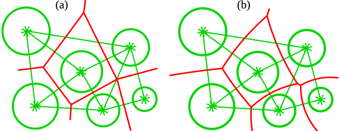
Figure 3: Comparison of two generalized Voronoi tessellations from the same set of generators. While the difference method (a) yields polygonal cells the quotient method (b) yields cells with piecewise spherical boundaries. In both cases, the weights are given by $w_{i}=r_{i}$. The cells are described by their cell center (green star) and their body (thick green circles). The Voronoi borders between cells are red lines, while the neighbor relations (i.e. those cells that share a common border) are indicated by thin green lines connecting their centers.

2.2 Quotient method

In the previous section it was found that, with subtractive weights in the $\mathcal{P}$-distance of the generalized Voronoi tessellation, the emerging cell contact border are planar surfaces. In contrast, if one divides the Euclidean distance by weights, then the cell contacts are spherical with the generalized square distance function defined as

$$\mathcal{P}_{i}(\mathbf{x})=\frac{(\mathbf{x}-\mathbf{x}_{i})^{2}}{w_{i}^{2}}.$$ (10)

Having its roots in computational geometry (see [7] and references therein), this method was introduced as a model for attraction domains of restaurants [6] more than 20 years ago. To our knowledge, it so far has not been used for physical or biological applications.

For simplicity of calculation, let the midpoint $\mathbf{x}_{ij}:=0$ be the origin of the coordinate system, while $\hat{\mathbf{d}}_{ij}$ remains the oriented cell-cell axis (see figure 4).

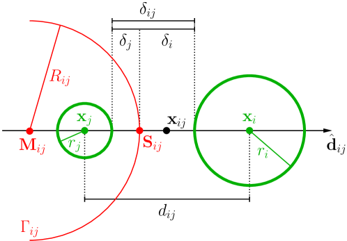
Figure 4: Geometry of cell pair and its pair contact border using the quotient method. In contrast to the difference method, this contact border $\Gamma_{ij}$ is a sphere around $\mathbf{M}_{ij}$ with radius $R_{ij}$. Its two-dimensional section is drawn in a red line.

Starting from $\mathcal{P}_{i}(\mathbf{x})=\mathcal{P}_{j}(\mathbf{x})$ with $w_{i}\neq w_{j}$ one arrives at the equivalent condition

$$\left(\mathbf{x}-\mathbf{M}_{ij}\right)^{2}=R_{ij}^{2}$$ (11)

for the point $\mathbf{x}$ to be on the border $\Gamma_{ij}$. Clearly, equation (11) describes an $n$-sphere around

$$\mathbf{M}_{ij}=-\frac{w_{i}^{2}+w_{j}^{2}}{w_{i}^{2}-w_{j}^{2}}\mathbf{x}_{i}\qquad\text{with radius}\qquad R_{ij}=\frac{w_{i}w_{j}}{(w_{i}^{2}-w_{j}^{2})}d_{ij},$$ (12)

where $d_{ij}=|\mathbf{x}_{i}-\mathbf{x}_{j}|=2|\mathbf{x}_{i}|$, resulting in a so called circular Voronoi tessellation. Assuming $r_{i}>r_{j}$ (as in figure 4), also the weights fulfill $w_{i}>w_{j}$ according to our monotonicity assumption on $w_{i}=w(r_{i})$. Thus, from equation (12) the center $\mathbf{M}_{ij}$ of the hypersphere $\Gamma_{ij}$ is always situated on the side of the cell $j$ with the smaller radius $r_{j}$. The contact sphere intersects the cell center connection segment $\overline{\mathbf{x}_{j},\mathbf{x}_{i}}$ at a unique contact point determined by

$$\mathbf{S}_{ij}\cdot\hat{\mathbf{d}}_{ij}=-\frac{w_{i}-w_{j}}{w_{i}+w_{j}}\cdot\frac{d_{ij}}{2}.$$ (13)

Similar as for the difference method (see figure 2), $\mathbf{S}_{ij}$ is situated on the side of the smaller cell body from the mid point $\mathbf{x}_{ij}=0$. Thus, the contact sphere contains the body of the cell with smaller weight, as indicated in figure 4. Once both weights are equal, equation (3) and thereby equation (13) simplify to

$$\mathbf{x}\cdot\hat{\mathbf{d}}_{ij}=\mathbf{S}_{ij}\cdot\hat{\mathbf{d}}_{ij}=0\qquad\text{for}\;\,w_{i}=w_{j},$$ (14)

revealing $\Gamma_{ij}$ as the classical Voronoi bisector line without weights.

In analogy to Lemma 1 for the difference method, we obtain the same unique specification of weight functions here as well:

Lemma 2.

Let $\{\mathcal{V}_{i},\Gamma_{ij}\}$ be a Voronoi tessellation of non-overlapping generators $\{g_{i}=(\mathcal{B}_{r_{i}}(\mathbf{x}_{i}),w_{i})\}$ constructed from $\mathcal{P}_{i}$ according to the quotient method in definition (10) with positive weights $w_{i}$. Then the inequalities (7) are satisfied for all cell pairs $i\neq j$ with arbitrarily small but positive cell body distance $\delta_{ij}=\delta_{i}+\delta_{j}$ if and only if

$$\forall i:\quad w_{i}=r_{i}.$$ (15)

Proof.

: The contact border equation $\mathcal{P}_{i}=\mathcal{P}_{j}$ evaluated for the point $\mathbf{x}=\mathbf{S}_{ij}$, see figure 4, yields $(r_{i}+\delta_{i})/w_{i}=(r_{j}+\delta_{j})/w_{j}$. Together with $\delta_{i}+\delta_{j}=\delta_{ij}$ we obtain the representation

$$\delta_{i}=\delta_{ij}\frac{w_{i}}{w_{i}+w_{j}}+\frac{r_{j}w_{i}-r_{i}w_{j}}{w_{i}+w_{j}}>0.$$ (16)

Since $\delta_{ij}>0$ can be arbitrarily small for fixed $r_{i},r_{j}$ and $w_{i},w_{j}$, the condition $\delta_{i}>0$ implies $r_{i}w_{j}\geq r_{j}w_{i}$. By exchanging $i$ and $j$, the second condition $\delta_{j}>0$ enforces equality and the existence of a joint positive constant with

$$w_{k}=r_{k}\cdot C\quad\text{for}\quad k=i,j.$$

Since the definition 1 of a Voronoi cell is independent of such a multiplicative constant in equation (10), we can set $C=1$ and obtain the result of the lemma. ∎

Thus, further on we can choose the weights $w_{i}=r_{i}$ when using the quotient method. Then the cell bodies are characterized as $\mathcal{B}_{r_{i}}(\mathbf{x}_{i})=\{\mathbf{x}:\,\mathcal{P}_{i}(\mathbf{x})<1\}$, so that inequality (4) is fulfilled under the assumption $\overline{\mathcal{B}_{r_{i}}(\mathbf{x}_{i})}\cap\overline{\mathcal{B}_{r_{j}}(\mathbf{x}_{j})}=\emptyset$. The emerging circular Voronoi tessellation is illustrated in figure 3(b). Rewriting equation (16) for i and j yields

$$\delta_{i,j}=\delta_{ij}\frac{r_{i,j}}{r_{i}+r_{j}},$$

and thus the regular partition property

$$\frac{\delta_{j}}{\delta_{i}}=\frac{r_{j}}{r_{i}},$$ (17)

meaning that the partition of the distance between cell bodies $\mathcal{B}_{r_{i}}(\mathbf{x}_{i})$ and $\mathcal{B}_{r_{j}}(\mathbf{x}_{j})$ by the contact arc is proportional to the ratio of body radii. Most importantly, in contrast to the difference method, the $\mathcal{P}$-distance in equation (10) ensures that $\delta_{i}$ monotonically increases with $r_{i}$, while $\delta_{j}=\delta_{ij}-\delta_{i}$ decreases, if $r_{j}>0$ and $\delta_{ij}>0$ are held fixed. As a consequence, the cell $i$ grows with increasing $r_{i}$. This property can also be observed for in-vivo cell monolayers,

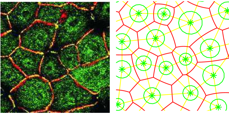
Figure 5: Typical microscopic picture of an epithelial monolayer (left) cultured of human keratinocytes, cell nuclei (green, black) and cell-cell contacts (yellow, red) are visualized by suitable staining (reproduced from [31]). In the simulated cell tissue (right) the sizes and positions of cell bodies (green) have been roughly adapted to deliver the observed contact arcs (red).

see figures 1, 5 and figure 5E in [44]. Thus, for the further discussions in this paper, the quotient method will be used exclusively to define Voronoi cells. Yet the tessellation is still unbounded due to infiniteness of marginal cells.

2.3 Closure of the Voronoi tessellation

In order to avoid infinitely extended cells at the tissue margin, the initial definition 1 of a Voronoi cell has to be modified. To this end, the method of finite closure for the difference method, as used by Drasdo and coworkers [18, 21], is extended to be generally applicable.

Definition 3.

Let $\mathcal{P}_{\mathrm{max}}\in\mathbb{R}^{+}$. The finite Voronoi cell of a generator $(\mathcal{B}_{r_{i}}(\mathbf{x}_{i}),w_{i}>0)$ is defined as

$$\mathcal{V}_{i}=\left\{\mathbf{x}\in\mathbb{R}^{n}:\mathcal{P}_{i}(\mathbf{x})<\min{\left(\mathcal{P}_{j}(\mathbf{x}),\mathcal{P}_{\mathrm{max}}\right)}\quad\forall j\neq i\right\}.$$ (18)

The exterior boundary closing a marginal $\mathcal{V}_{i}$ is

$$\Gamma_{i0}=\left\{\mathbf{x}\in\mathbb{R}^{n}:\mathcal{P}_{i}(\mathbf{x})=\mathcal{P}_{\mathrm{max}}\right\}\setminus\bigcup_{j\neq i}\mathcal{V}_{j},$$ (19)

and the total boundary of the Voronoi neighborhood around $\mathbf{x}_{i}$ is

$$\partial\mathcal{V}_{i}=\Gamma_{i0}\cup\bigcup_{j\neq i}\Gamma_{ij},$$

where now the contact border between cell $i$ and $j$ is given by

$$\Gamma_{ij}=\Bigl{\{}\mathbf{x}\in\mathbb{R}^{n}:\;\mathcal{P}_{i}(\mathbf{x})=\mathcal{P}_{j}(\mathbf{x})\leq\min\bigl{(}\mathcal{P}_{k}(\mathbf{x}),\mathcal{P}_{\mathrm{max}}\bigr{)}\quad\forall k\neq i,j\Bigr{\}}.$$ (20)

For any choice of $\mathcal{P}_{\mathrm{max}}>0$, the Voronoi tessellation generated from a finite set of cell bodies $\{(\mathcal{B}_{r_{i}}(\mathbf{x}_{i}),w_{i})\}$ comprises a bounded region of the whole space, representing a cell tissue of finite extension. In figure 6 we depict the model representation of an

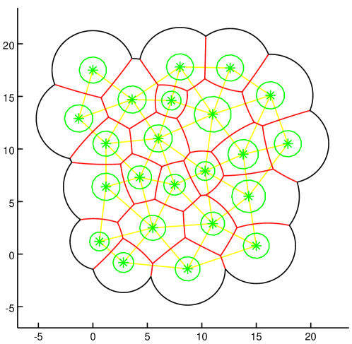
Figure 6: Model representation of a bounded cell monolayer using the quotient method with $\mathcal{P}_{\mathrm{max}}$-cutoff. Axis tics are in units of $\mu\mathrm{m}$.

in vivo cell monolayer (see figure 5) generated by the quotient method using definition (10) with $w_{i}=r_{i}$. The exterior boundaries $\Gamma_{i0}$ of the Voronoi neighborhoods for marginal cells are circular arcs drawn as black lines. Apparently the size of a cell $i$ is influenced by the two parameters $r_{i}$ and $\mathcal{P}_{\mathrm{max}}$. While $\mathcal{P}_{\mathrm{max}}$ regulates the overall cell size by globally scaling each $r_{i}$, the ratios $r_{i}/r_{j}$ determine the partition of space between each cell pair $i,j$ by specifying the actual position of $\Gamma_{ij}$. We remark that both $\mathcal{P}_{\mathrm{max}}$ and $\{r_{i}\}$ are accessible to experimental determination using image analysis tools, see figure 5 and especially figure 1(c).

The necessary condition $\mathcal{P}_{i}(\mathbf{x})<\mathcal{P}_{\mathrm{max}}$ for a point $\mathbf{x}$ to be within cell $i$ defines a ball $\mathcal{B}_{R_{i0}}(\mathbf{x}_{i})$ around $\mathbf{x}_{i}$, which will be called free ball further on. It has the squared radius $R_{i0}^{2}=w_{i}^{2}+\mathcal{P}_{\mathrm{max}}$ in the difference method and $R_{i0}^{2}=w_{i}^{2}\cdot\mathcal{P}_{\mathrm{max}}$ in the quotient method. As illustrated in figure 7,

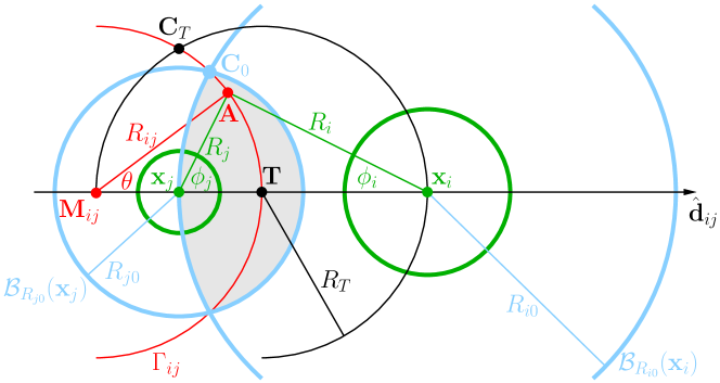
Figure 7: Maximal $\mathcal{P}$-distance $\mathcal{P}_{\mathrm{max}}$ and its effect on the neighbor relation of two cells $i,j$. The cells $i,j$ can only share a common $\Gamma_{ij}$ and thus be neighbors, if there is a non-empty overlap region (shaded) given by the intersection of their free balls $\mathcal{B}_{R_{i0}}(\mathbf{x}_{i}),\mathcal{B}_{R_{j0}}(\mathbf{x}_{j})$ (blue outer circles). The other quantities are explained in the text.

this has the effect that two cells $i,j$ can only be neighbors, if their free balls $\mathcal{B}_{R_{i0}}(\mathbf{x}_{i}),\mathcal{B}_{R_{j0}}(\mathbf{x}_{j})$ overlap. In case of no contact, $\mathcal{V}_{i}=\mathcal{B}_{R_{i0}}(\mathbf{x}_{i})$ represents an isolated spherical cell, which clearly has to include its cell body $\mathcal{B}_{r_{i}}(\mathbf{x}_{i})$. Thus, the condition

$$r_{i}^{2}<R_{i0}^{2}=\left\{\begin{aligned} &r_{i}^{2}+\mathcal{P}_{\mathrm{max}}\;&\text{(difference method)}\\ &r_{i}^{2}\cdot\mathcal{P}_{\mathrm{max}}\;&\text{(quotient method)}\end{aligned}\right.$$ (21)

is imposed, meaning that $\mathcal{P}_{\mathrm{max}}$ has to be chosen so that

$$\mathcal{P}_{\mathrm{max}}>0\quad\text{(difference method)}$$ (22)

$$\mathcal{P}_{\mathrm{max}}>1\quad\text{(quotient method)}.$$

In this way, the larger $\mathcal{P}_{\mathrm{max}}$, the larger is the radius of isolated cells relative to their cell body.

Within the difference method, this $\mathcal{P}_{\mathrm{max}}$-closure is straight-forward because the planar cell contacts lead to starlike (even convex) Voronoi cells $\mathcal{V}_{i}$. Recall the definition of starlikeness with respect to the center $\mathbf{x}_{i}$: $\forall\mathbf{x}\in\mathcal{V}_{i}$ also $\overline{\mathbf{x}_{i}\mathbf{x}}\subset\mathcal{V}_{i}$. In fact, a $\mathcal{P}_{\mathrm{max}}$-closed generalized Voronoi tessellation has been applied to epithelial tissue modeling by prescribing $\mathcal{B}_{R_{i0}}(\mathbf{x}_{i})$ for each cell [21]. However, within the quotient method the situation is more complicated. In analogy to the difference method it is reasonable to require that the Voronoi cells $\mathcal{V}_{i}$ are star-like domains with respect to $\mathbf{x}_{i}$. In order to ensure starlike cells within the quotient method, $\mathcal{P}_{\mathrm{max}}$ must not be chosen too large. Consider the cell pair as sketched in figure 7. The straight line connecting $\mathbf{x}_{i}$ and $\mathbf{C}_{T}$ is a tangent to $\Gamma_{ij}$. Thus it is clear from the geometry that both $\mathcal{V}_{i}$ and $\mathcal{V}_{j}$ are star-like domains with respect to $\mathbf{x}_{i},\mathbf{x}_{j}$, if their corresponding free balls $\mathcal{B}_{R_{i0}}(\mathbf{x}_{i}),\mathcal{B}_{R_{j0}}(\mathbf{x}_{j})$ do not extend beyond the point $\mathbf{C}_{T}$. Before we proceed, we introduce the cell size homogeneity quotient

$$Q=\min_{i,j}\frac{r_{i}+r_{j}}{|r_{i}-r_{j}|}=\frac{r_{\text{max}}+r_{\text{min}}}{r_{\text{max}}-r_{\text{min}}},$$ (23)

where the last equality follows from monotonicity arguments. Therefore, $Q=Q(\{r_{i}:i=1\dots N\})$ is a measure of the uniformity of cell sizes within a tissue, with $Q=\infty$ for equal $r_{i}$ and $Q\approx 1$ for $r_{\text{max}}>>r_{\text{min}}$.

Proposition 1 (Starlike cells).

For a finite Voronoi tessellation generated from non-overlapping $\{\mathcal{B}_{r_{i}}(\mathbf{x}_{i})\}$ by using the quotient method in definition (10) with weights $w_{i}=r_{i}$, the resulting Voronoi cells $\mathcal{V}_{i}$ are starlike with respect to $\mathbf{x}_{i}$, if the maximal $\mathcal{P}$-distance $\mathcal{P}_{\mathrm{max}}$ fulfills the homogeneity constraint

$$1<\mathcal{P}_{\mathrm{max}}\leq Q.$$ (24)

This condition on the tissue properties will be crucial later on and guarantees that each actin fiber bundle emanating radially from $\partial\mathcal{B}_{r_{i}}(\mathbf{x}_{i})$ intersects the boundary $\partial\mathcal{V}_{i}$ only once, see figure 9.

Proof.

: From fundamental trigonometric relations follows the angle $\angle(\mathbf{T},\mathbf{x}_{j},\mathbf{C}_{T})$, namely

$$\phi_{j}^{T}=\frac{\pi}{2},$$ (25)

and geometric similarity of the triangles $\triangle(\mathbf{M}_{ij},\mathbf{x}_{i},\mathbf{C}_{T}),\triangle(\mathbf{x}_{i},\mathbf{C}_{T},\mathbf{x}_{j})$. Thus, with $r_{j}<r_{i}$, we have for point $\mathbf{A}=\mathbf{C}_{T}$

$$\cos\theta_{T}=\frac{r_{j}}{r_{i}}$$ (26)

$$R_{jT}=\frac{r_{j}}{\sqrt{|r_{i}^{2}-r_{j}^{2}|}}\cdot d_{ij},\qquad R_{iT}=\frac{r_{i}}{\sqrt{|r_{i}^{2}-r_{j}^{2}|}}\cdot d_{ij}.$$ (27)

With the last two equations, the maximal distances of a point $\mathbf{A}$ on $\Gamma_{ij}$ from the cell centers have been identified for each cell pair. Starlikeness of $\mathcal{V}_{i}$ is equivalent to the condition $R_{i0}^{2}\leq R_{iT}^{2}$, where $R_{i0}^{2}=\mathcal{P}_{\mathrm{max}}r_{i}^{2}$, so that $\mathcal{P}_{\mathrm{max}}\leq d_{ij}^{2}/|r_{i}^{2}-r_{j}^{2}|$, which can be fulfilled by requiring $\mathcal{P}_{\mathrm{max}}\leq Q$, since $\forall i,j:\;(r_{i}+r_{j})^{2}\leq d_{ij}^{2}$. With the condition (22) the assertion follows. ∎

In particular, starlikeness prohibits engulfment of one cell by the other, so that $\mathcal{B}_{R_{i0}}(\mathbf{x}_{i})$ may not contain $\mathcal{B}_{R_{j0}}(\mathbf{x}_{j})$ completely for $r_{i}>r_{j}$. Note that within sufficiently large tissues, the smallest and biggest cell will usually not be in contact, which relaxes inequality (24) into the condition:

$$1<\mathcal{P}_{\mathrm{max}}\leq\min_{\text{\rm neighbors}\;i,j}\frac{r_{i}+r_{j}}{|r_{i}-r_{j}|}=:Q_{\mathrm{nb}}.$$ (28)

In such a circular Voronoi diagram there may be $\mathcal{O}(N^{2})$ cell-cell contacts and vertices, in particular for low cell size homogeneity quotients $Q$. The supplementary material contains the extensively commented GNU octave routine mwvoro.m (Matlab compatible) used to create and visualize a circular closed Voronoi tessellation, together with configuration and plotting facilities. The partition of space into distinct cells and their neighborhood relations has an algorithmic complexity of $\mathcal{O}(N^{2})$, $N$ being the number of cells. Due to the extension of closing marginal cells by $\mathcal{P}_{\mathrm{max}}$-arcs, we do not follow the method proposed by Aurenhammer and Edelsbrunner [7]. In particular, we do not use polyedral “cell complexes” in an inverted three-dimensional embedding of the Voronoi generators. Nevertheless we retain the same optimal algorithmic complexity.

3 Cell shape and dynamics

When a single cell is placed on a two-dimensional and adhesive substratum, it usually spreads into all directions attaining a circular shape like a fried egg, as can be observed in figure 8.

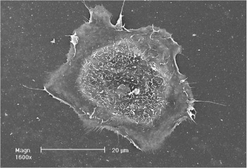
Figure 8: Electron microscopic picture of a keratinocyte (courtesy of Gregor Wenzel). There are two distinct regions within the cell. An inner, more dense region with ruffled membrane structures appearing in white (cell body), and an outer, flat region with larger ruffles or filopodia near the cell margin (lamella), which in the case of no contact with other cells forms a ring of more or less constant diameter around the cell body. See also figure 1.

Thereby, the exterior visco-elastic lamella along the free boundary $\Gamma_{i0}$, which consists of parts of $\mathcal{B}_{R_{i0}}(\mathbf{x}_{i})$, supports the protruding and retracting cell edge. This smooth flat region contains a network of dynamic actin filaments situated around the inner, almost solid cell body $\mathcal{B}_{r_{i}}(\mathbf{x}_{i})$, see e.g. [1, 40]. The maximal spreading radius $R_{i0}=\sqrt{\mathcal{P}_{\mathrm{max}}}\cdot r_{i}$ is determined by the strength of adhesion to the substrate and the equilibrium between protrusive activity at the cell periphery $\Gamma_{i0}$ and the contractile retrograde actin flow [30]. Assuming that for given adhesiveness the averaged local cytoskeletal network volume fraction ($\theta$ in [30]) in the lamellae has a certain value $q_{0}$ independent of cell size, the weighting of $R_{i0}$ proportional to the cell body radius follows.

Usually, the irregular activity of living cells at their lamella edge leads to a curled cell boundary, see figures 1(c) and 8. Neglecting fluctuations on short time $\mathcal{O}(10s)$ and length scales $\mathcal{O}(1\mu\mathrm{m})$, the free portions of the cell edge $\Gamma_{i0}$ are approximately taken as circular in this model. The actual cell edge fluctuates within the vicinity of the smooth arcs, representing the averaged position of the plasma membrane, and will later on be taken as the source of stochastic perturbation forces, see section 3.4. Thus, in our model the active lamella region of a single free cell is approximately ring shaped and has a width of

$$\delta_{i0}=(\sqrt{\mathcal{P}_{\mathrm{max}}}-1)r_{i}.$$ (29)

Once two epithelial cells $i,j$ come close enough to interact, the two adjoining lamellae compete for the occupation of the region in between them. Eventually they form a contact border, which exhibits microscopic fluctuations due to local plasma membrane flickering. Yet it approximately attains the shape of a circular arc, whereby small gaps between the two cell membranes are neglected. This experimental fact (see e.g. corresponding figures in [49, 31, 44] and 5, 1 in this article) is well represented by the Voronoi border $\Gamma_{ij}$ resulting from the quotient method defined by equation (10). In this way, within our tissue model, the cell boundaries are merely composed of piecewise circular arcs, and the cell bodies are not necessarily located in the middle of the cells. By suitable choice of $w_{i}$ (Lemma 2) there is always some lamella region separating the cell body from the neighbor cell ($\delta_{i}>0$, also cf. figure 4).

3.1 Interaction forces between cells

The cytoskeleton with its network of filaments often features bundled structures, which are commonly visible as so-called stress fibers, emanating from the cell body or nucleus in radial direction. According to [1], bundles of filamentous actin attach to transmembrane complexes called adherens junctions, which are made from e.g. catenins on the cytosolic side and cadherins at the exterior of the cell. Furthermore, intermediate filaments such as the rope-like keratin tie in with rivet-like desmosomes at the cell membrane. By connecting neighboring cells, these structures stiffen and strengthen the tissue coherence. For example, in certain epithelia, cadherin-catenin adherens junctions comprise a whole transcellular adhesion belt.

Inspired by this observation, it is assumed that the attractive force between two cell bodies $\mathcal{B}_{r_{i}}(\mathbf{x}_{i}),\mathcal{B}_{r_{j}}(\mathbf{x}_{j})$ is transduced by radial filament structures extending towards the cell boundaries. Thereby, the filaments of one cell connect to those of the other and form pairs along the contact border $\Gamma_{ij}$. Thus, the intercellular adherens junctions emerge according to the respective filament densities as emanating from cell $i$ and $j$, respectively (see figure 9).

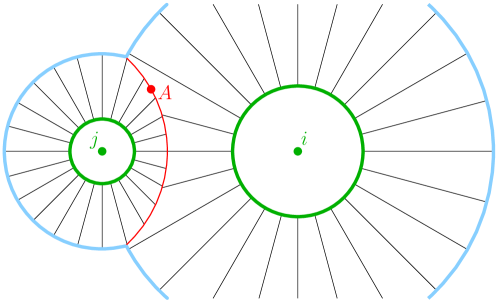
Figure 9: Pairing of filaments from one cell to the other cell. For the definition of symbols and angles to describe the geometry of pairing filaments of a neighboring cell pair see figure 7.

Furthermore, the connecting cell-cell junctions are not fixed but undergo dissociation, diffusion, and renewed association. Motivated by protein (e.g. cadherin) diffusion properties in membranes [22, 12], this process is considered to be fast (seconds) compared to the slower time scale (several minutes) of cell deformation and translocation. In this way, pair formation of cross-attachments between filament bundles from both cell bodies can be regarded as a pseudo-stationary stochastic process [19]. In order to compute the interaction force between two cells, one needs a suitable expression for the density of pairing filaments $\rho(\theta)$ at the border of the cells $i,j$.

3.2 Filament pair density at cell-cell contacts

Consider the cell pair as illustrated in figures 7 and 9 with cell body radii $r_{i}>r_{j}$ and the distinguished Voronoi weights as in equation (15). Let $\theta$ parameterize the contact arc $\Gamma_{ij}$ given by $\mathbf{M}_{ij},R_{ij}$, and let $\mathbf{A}$ be the corresponding point upon that arc. Starting from the surface of the cell bodies $\mathcal{B}_{r_{i}}(\mathbf{x}_{i})$ and $\mathcal{B}_{r_{j}}(\mathbf{x}_{j})$, filaments extend in radial direction under angles $\phi_{i}(\theta)$ and $\phi_{j}(\theta)$, respectively, to eventually meet at $\mathbf{A}$. Furthermore, let $R_{i}$ and $R_{j}$ denote the distances between the cell centers and $\mathbf{A}$. The density of filaments is assumed to be constant on the surface of each cell body, given by a universal value $\tilde{\rho}>0$. In order to construct the pairing density of filaments $\rho(\theta)$ along the contact surface, these cell body surface densities are mapped onto $\Gamma_{ij}$ by equating the corresponding surface elements

$$\rho_{i}(\theta)R_{ij}\mathrm{d}\theta=\tilde{\rho}r_{i}\mathrm{d}\phi_{i},\qquad\rho_{j}(\theta)R_{ij}\mathrm{d}\theta=\tilde{\rho}r_{j}\mathrm{d}\phi_{j}.$$ (30)

With $\mathbf{A}=\mathbf{A}(\theta)\in\Gamma_{ij}$, (cf. figures 7 and 9), it holds

$$R_{ij}\sin{\theta}=R_{i}\sin{\phi_{i}}=R_{j}\sin{\phi_{j}}$$ (31)

$$R_{ij}\cos{\theta}=|\mathbf{x}_{j}-\mathbf{M}_{ij}|+R_{j}\cos{\phi_{j}}.$$ (32)

The defining condition for the contact border in equation (3) can be written as

$$R_{j}=\eta R_{i}\qquad\text{with}\;\eta=\frac{w_{j}}{w_{i}}=\frac{r_{j}}{r_{i}}<1.$$ (33)

Thus, from equation (31) we obtain the simple relation

$$\sin{\phi_{i}}=\eta\cdot\sin{\phi_{j}}$$ (34)

between the two angles $\phi_{i}(\theta)$ and $\phi_{j}(\theta)$, so that differentiation with respect to $\theta$ yields the proportionality

$$\frac{\mathrm{d}\phi_{i}}{\mathrm{d}\theta}=\eta\cdot\frac{\cos{\phi_{j}}}{\cos{\phi_{i}}}\cdot\frac{\mathrm{d}\phi_{j}}{\mathrm{d}\theta}=\frac{\eta}{\kappa_{\eta}(\phi_{j})}\cdot\frac{\mathrm{d}\phi_{j}}{\mathrm{d}\theta},$$ (35)

where $\kappa_{\eta}(\phi_{j})=\sqrt{1+(1-\eta^{2})\cdot\tan^{2}\phi_{j}}$. Moreover, by solving equation (31) for $R_{j}$ in terms of $R_{ij}$, inserting it into equation (32), and using the relations (12) we get an explicit expression for $\tan{\phi_{j}}$ in terms of $\theta$

$$\tan{\phi_{j}}=\frac{\sin{\theta}}{\cos{\theta}-\eta},$$ (36)

which holds for all $|\theta|<\theta_{T}$, with $\cos\theta_{T}=\eta$, or equivalently, $|\phi_{j}|<\pi/2$, see equations (25,26). Finally, by differentiation of equation (36) with respect to $\theta$ we obtain

$$\frac{\mathrm{d}\phi_{j}}{\mathrm{d}\theta}=\frac{\tan{\phi_{j}}}{1+\tan^{2}\phi_{j}}\cdot\biggl{(}\tan{\phi_{j}}+\frac{1}{\tan{\theta}}\biggr{)}=\frac{1-\eta\cos{\theta}}{1-2\eta\cos{\theta}+\eta^{2}}>0.$$ (37)

It is assumed, that the pairing density function $\rho(\theta)$, depending on $\rho_{i}(\theta)$ and $\rho_{j}(\theta)$, is even in $\theta$, maximal at $\theta=0$, and strictly monotonically decreasing for increasing $|\theta|$. Here, two exemplary models to specify such a density function $\rho(\theta)$ are discussed:

Model 1: Minimal density pairing.

If locally one cell has less filaments binding to $\Gamma_{ij}$ than the other, then there will be a pairing match for all of its filaments. Thus, the local density of pairs on $\Gamma_{ij}$ will equal the lower filament density:

$$\rho(\theta)=\min\Bigl{(}\rho_{i}(\theta),\rho_{j}(\theta)\Bigr{)}=\frac{\tilde{\rho}}{R_{ij}}\min\biggl{(}r_{i}\frac{\mathrm{d}\phi_{i}}{\mathrm{d}\theta},r_{j}\frac{\mathrm{d}\phi_{j}}{\mathrm{d}\theta}\biggr{)},$$ (38)

where we used the identities (30). With $\kappa_{\eta}>0$ we conclude from equation (35) that $\rho(\theta)=\rho_{i}(\theta)\leq\rho_{j}(\theta)$. Therefore, an explicit representation of $\rho$ in terms of $\phi_{j}$ and its derivative is

$$\rho_{\text{min}}(\theta)=\rho_{i}(\theta)=\tilde{\rho}\cdot\frac{r_{j}}{R_{ij}\cdot\kappa_{\eta}(\phi_{j})}\cdot\frac{\mathrm{d}\phi_{j}}{\mathrm{d}\theta}.$$

The emerging behavior of $\rho(\theta)$ is visualized in figure 10,

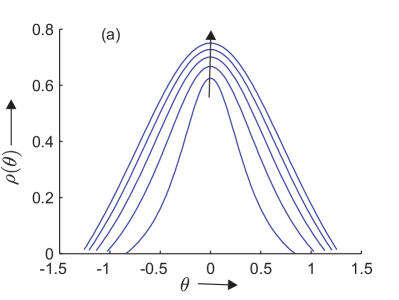
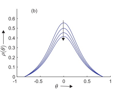
Figure 10: Plot of density function $\rho(\theta)$, described by model 1 (minimal density pairing). (a): The distance of cell bodies $\delta_{ij}>0$ and $r_{j}>0$ are fixed constants, while $r_{i}>r_{j}$ successively increases. (b): $r_{i}>r_{j}>0$ are fixed constants, while the distance of cell bodies successively increases.

where the maximal angle $\theta_{T}$, as found before in equation (26), can be clearly seen in plot (b). It does not appear so prominent in plot (a), where it varies with $r_{i}$.

Model 2: Mean density pairing.

Assuming that each filament from either of the neighboring cells has a probability to randomly form a pair at some junction on $\Gamma_{ij}$, the resulting pairing density can be defined as the geometric mean of $\rho_{i}$ and $\rho_{j}$:

$$\rho_{\text{mean}}(\theta)=\sqrt{\rho_{i}(\theta)\cdot\rho_{j}(\theta)}=\tilde{\rho}\cdot\frac{r_{j}}{R_{ij}\cdot\sqrt{\kappa_{\eta}(\phi_{j})}}\cdot\frac{\mathrm{d}\phi_{j}}{\mathrm{d}\theta}.$$ (39)

In figure 11 the emerging behavior of $\rho(\theta)$ is visualized, showing an even more expressed cut-off at $\theta=\theta_{T}$

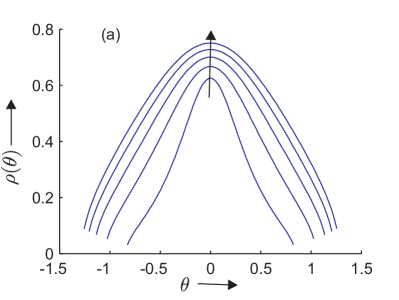
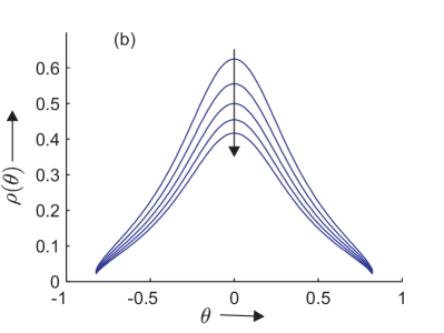
Figure 11: Plot of density function $\rho(\theta)$, described by model 2 (mean density pairing). (a): The distance of cell bodies $\delta_{ij}>0$ and $r_{j}>0$ are fixed constants, while $r_{i}$ successively increases. (b): $r_{i}>0$ and $r_{j}>0$ are fixed constants, while the distance of cell bodies $\delta_{ij}$ successively increases.

From figures 10 and 11 it becomes apparent that $\rho(\theta)$ is even in $\theta$, maximal for $\theta=0$, and strictly decreasing for increasing $|\theta|$ in both methods. Whereas model 1 captures the maximal filament pairing that could be realized for long term association at fixed adherens junctions, model 2 describes the pseudo-steady state of short term stochastic filament association, which will be considered further on.

3.3 Pair interaction force

Consider two cells $i,j$ touching each other, so that if their cell body distance $\delta_{ij}=\delta_{i}+\delta_{j}$ was further increased, they would dissociate. By equation (29) this limiting rupture distance $\delta_{ij}^{\mathrm{(rup)}}$ is given as

$$\delta_{ij}^{\mathrm{(rup)}}=\delta_{i0}+\delta_{j0}=\bigl{(}\sqrt{\mathcal{P}_{\mathrm{max}}}-1\bigr{)}(r_{i}+r_{j}).$$ (40)

Then according to the previous assumptions, any paired couple of actin fibers meeting at an adherens junction in the contact boundary $\Gamma_{ij}$ near the intersection point $\mathbf{S}_{ij}$ (see figure 4) develops a certain positive stress between the two cell bodies. According to the assumption made at the beginning of this chapter, this stress depends on the mean volume fraction $q_{0}$ of the contractile cytoskeletal network, which before touching was equal in both contacting lamellae of width $\delta_{i0},\delta_{j0}$, respectively. If now $\delta_{ij}$ further decreases, then both lamellae will be compressed by the equal factor $\delta_{i}/\delta_{i0}=\delta_{j}/\delta_{j0}=\delta_{ij}/\delta_{ij}^{\mathrm{(rup)}}<1$ as a consequence of the Voronoi partition laws (18) and (19). Thus, we can suppose that (a) the mean volume fraction in both lamellae increases to the same value $q$ satisfying the inverse relation

$$\frac{q}{q_{0}}=\frac{\delta_{ij}^{\mathrm{(rup)}}}{\delta_{ij}},$$ (41)

and (b) any paired actin fibers develop the same stress between their adherens junction and the corresponding cell body, with a strength $\tilde{f}=f(q)$ that, for simplicity, depends only on the common cytoskeletal volume fraction $q$. Since the cytoskeletal network consists not only of cross-linked actin-myosin filaments but also of more or less flexible microtubuli and intermediate filaments (as keratin, for example) [29, 42, 40, 1], the stress function $f(q)$ has to decrease to (large) negative values for increasing $q\rightarrow q_{\text{max}}=1$. Here we chose the simple, thermodynamically compatible strictly decreasing model function

$$f(q)=f_{\mathrm{int}}\Bigl{(}\ln(1-q)-\ln q-\ln z_{c}\Bigr{)}.$$

The corresponding convex generalized free energy $\mathcal{F}$ satisfies

$$\mathcal{F}(1-q)=(1-q)\Bigl{(}f(q)-f_{\mathrm{int}}\Bigr{)}$$

for $0<q<1$ (cf. [2]), where the positive constant $z_{c}<1/q_{0}-1$ determines the critical volume fraction $q_{c}=1/(1+z_{c})>q_{0}$ such that $f(q_{c})=0$. Applying transformation (41) we finally obtain an actin fiber stress function that depends only on the relative cell body distance $\Delta_{ij}=\delta_{ij}/\delta_{ij}^{\mathrm{(rup)}}<1$, namely

$$f(\Delta_{ij})=f_{\mathrm{int}}\cdot\ln\Bigl{(}\frac{\Delta_{ij}-\Delta_{\mathrm{min}}}{\Delta_{\mathrm{crit}}-\Delta_{\mathrm{min}}}\Bigr{)},$$ (42)

where $0<\Delta_{\mathrm{min}}=q_{0}<q_{0}(1+z_{c})=\Delta_{\mathrm{crit}}<1$.

The derivation of this stress model relies on the simplifying assumption that according to equation (41) the stress of each paired filament extending from cell body $\mathcal{B}_{r_{i}}(\mathbf{x}_{i})$ to the adherens junction at $\Gamma_{ij}$ is completely determined by the adhesion strength (appearing as coefficient $f_{\mathrm{int}}$) and the cytoskeletal state $q$ of the intermediate lamella near the horizontal cell-cell connection axis in direction $\hat{\mathbf{d}}_{ij}$, see figures 7 and 9. Moreover, relative to this coordinate frame the paired filament orientations are $\hat{\mathbf{R}}_{i}=(-\cos\phi_{i},\sin\phi_{i})$ and $\hat{\mathbf{R}}_{j}=(\cos\phi_{j},\sin\phi_{j})$, so that the corresponding adherens junction at $\Gamma_{ij}$ experiences two force vectors $\mathbf{f}_{i}=-f(\Delta_{ij})\cdot\hat{\mathbf{R}}_{i}$ and $\mathbf{f}_{j}=-f(\Delta_{ij})\cdot\hat{\mathbf{R}}_{j}$ with opposing horizontal components. However, their resultant vector $\mathbf{f}_{i}+\mathbf{f}_{j}$ generally does not vanish (except for $\phi_{i}=\phi_{j}=0$). It has a negative vertical component $-f(\Delta_{ij})\cdot(\sin\phi_{i}+\sin\phi_{j})$, which could pull the adherens junction towards the cell-cell connection line along the contact boundary $\Gamma_{ij}$.

Therefore, some counterforces due to substrate adhesion via e.g. integrin [20, 23] or frictional drag have to be supposed in order to guarantee the assumed pseudo-stationary equilibrium condition for $\Gamma_{ij}$. Using the simplifying decomposition in horizontal and vertical components, we arrive at the following model expression for the force $\mathbf{f}_{ij}$ applied by a single filament pair onto the cell body center $\mathbf{x}_{j}$:

$$\begin{split}\mathbf{f}_{ij}&=\frac{1}{2}\bigl{(}\mathbf{f}_{i}-\mathbf{f}_{j}\bigr{)}^{\text{(hor)}}-\frac{\alpha}{2}\bigl{(}\mathbf{f}_{i}+\mathbf{f}_{j}\bigr{)}^{\text{(ver)}}\\ &=\frac{f(\Delta_{ij})}{2}\Bigl{(}(\cos\phi_{i}+\cos\phi_{j})\hat{\mathbf{d}}_{ij}+\alpha(\sin\phi_{i}+\sin\phi_{j})\hat{\mathbf{d}}_{ij}^{\perp}\Bigr{)},\end{split}$$ (43)

where $\alpha\geq 0$ is an additional adhesion or friction parameter. By relying on the pairing filament density $\rho(\theta)$ in section 3.2, we obtain an integral expression for the total pair interaction force applied by cell $i$ onto cell $j$:

$$\mathbf{F}_{ij}^{\mathrm{(int)}}=R_{ij}\int_{\Gamma_{ij}}\mathrm{d}\theta\;\rho(\theta)\cdot\mathbf{f}_{ij}(\theta)$$ (44)

where the trigonometric relations between $\phi_{i}$, $\phi_{j}$ and the parameterization angle $\theta$ have to be extracted from equations (30) – (33). Conversely, the force of cell $j$ onto $i$ is determined by the relations

$$F_{ji}^{\mathrm{(hor)}}=-F_{ij}^{\mathrm{(hor)}}\qquad F_{ji}^{\mathrm{(ver)}}=F_{ij}^{\mathrm{(ver)}}.$$ (45)

The emerging cell pair interaction force as described by equation (44) is shown in figures 12 and 13.

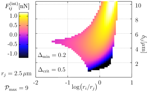
Figure 12: Modulus $F_{ij}^{\text{(int)}}$ of pair interaction force $\mathbf{F}_{ij}^{\mathrm{(int)}}$, see equation (44). In the empty regions of the plot, $\mathbf{F}_{ij}^{\mathrm{(int)}}$ is not defined. There, $\mathcal{B}_{R_{i0}}(\mathbf{x}_{i})\cap\mathcal{B}_{R_{j0}}(\mathbf{x}_{j})$ extends beyond $\Gamma_{ij}$ as bounded by $\theta_{T}$, or the cells are not in contact at all.

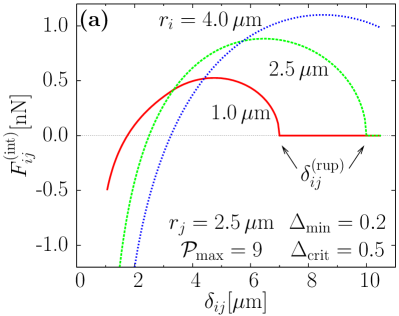
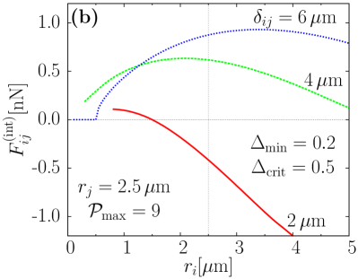
Figure 13: Modulus of pair interaction force $\mathbf{F}_{ij}^{\mathrm{(int)}}$ depending on (a) $\delta_{ij}$ and (b) $r_{i}$. The global view depending on both $\delta_{ij}$ and the logarithmic ratio $r_{i}/r_{j}$ was presented in figure 12.

A natural and maximal cut-off distance for the force is given by the finiteness of the Voronoi tessellation, whereby neighboring is only possible for sufficiently small cell center distances $\delta_{ij}<\delta_{ij}^{\mathrm{(rup)}}+r_{i}+r_{j}$, i.e. $\overline{\mathcal{B}_{R_{i0}}(\mathbf{x}_{i})}\cap\overline{\mathcal{B}_{R_{j0}}(\mathbf{x}_{j})}\neq\emptyset$. Once two previously isolated cells come close enough for contact, there is a strong tendency to attach, which facilitates multicellular tissue formation. The interaction force is attractive until the cell distance $\delta_{ij}$ reaches $\delta_{ij}^{\mathrm{(crit)}}=\Delta_{\mathrm{crit}}\cdot\delta_{ij}^{\mathrm{(rup)}}$, where $\mathbf{F}_{ij}^{\mathrm{(int)}}$ vanishes. Finally, if $\delta_{ij}$ drops below $\delta_{ij}^{\mathrm{(crit)}}$, $\mathbf{F}_{ij}^{\mathrm{(int)}}$ becomes repulsive and therefore hinders tissue collapse at distances approaching $\delta_{ij}^{\mathrm{(min)}}=\Delta_{\mathrm{min}}\cdot\delta_{ij}^{\mathrm{(rup)}}$. Note that with $\Delta_{ij}>\Delta_{\mathrm{min}}$ the lower bound from inequality (28) on the homogeneity of cell radii due to fixed $\sqrt{\mathcal{P}_{\mathrm{max}}}$ can be relaxed to

$$1<\frac{\mathcal{P}_{\mathrm{max}}}{\bigl{(}\Delta_{\mathrm{min}}(\sqrt{\mathcal{P}_{\mathrm{max}}}-1)+1\bigr{)}^{2}}\leq Q_{\mathrm{nb}}.$$ (46)

Correspondingly, $\mathcal{P}_{\mathrm{max}}$ can be increased for given cell homogeneity $Q$ or $Q_{\mathrm{nb}}$. For example, the constraint (46) yields $Q_{\mathrm{nb}}=6.25$ for $\sqrt{\mathcal{P}_{\mathrm{max}}}=3$, or $r_{\text{min}}\geq 0.73\cdot r_{\text{max}}$ for each cell pair. In fact, the actual distances $\Delta_{ij}$ in a tissue will be larger than $\Delta_{\mathrm{min}}$, effectively relaxing (46) even further.

3.4 Locomotion force at the free boundary

In addition to the dynamics induced by pair interaction forces, cells at the tissue margin may migrate into open space. The locomotion force causing such a migration is due to lamellipodial protrusion and retraction, which is unhindered only at the free cell boundary $\Gamma_{i0}$. In a similar manner as before, we assume that this locomotion or free boundary force onto the cell body $\mathcal{B}_{r_{i}}(\mathbf{x}_{i})$ is determined by connecting radial filament bundles as indicated in figure 9. The filament density of cell $i$ along its free boundary $\Gamma_{i0}$ is given by

$$\rho_{i0}=\frac{\tilde{\rho}r_{i}}{R_{i0}}=\frac{\tilde{\rho}}{\sqrt{\mathcal{P}_{\mathrm{max}}}},$$ (47)

and thus independent of $r_{i}$. In this way, the locomotive force of a cell $i$ reads as

$$\mathbf{F}_{i}^{\mathrm{(loc)}}=f_{\mathrm{loc}}\int_{\Gamma_{i0}}\mathrm{d}s_{i}\,\rho_{i0}\hat{\mathbf{R}}_{i0}(\phi_{i}),$$ (48)

with arc length $s_{i}=R_{i0}\phi_{i}$ and $\hat{\mathbf{R}}_{i0}(\phi_{i})=(\cos\phi_{i},\sin\phi_{i})$. Moreover, in order to heuristically account for ubiquitous perturbations due to lamellipodial fluctuations or possible signals, we implement stochastic force increments at the tissue margin

$$\mathrm{d}\mathbf{F}_{i}^{\mathrm{(st)}}=b_{0}\int_{\Gamma_{i0}}\mathrm{d}\mathbf{B}_{t,s_{i}}.$$ (49)

Here we assume a uniform and anisotropic vector noise $\mathbf{B}_{t,s_{i}}$ defining a spatio-temporal Brownian sheet in arc length and time coordinates with independent Gaussian increments satisfying $\operatorname{Var}\bigl{(}\mathrm{d}\mathbf{B}_{ts_{i}}\bigr{)}=\mathrm{d}s_{i}\cdot\mathrm{d}t$. For each time $t$, stochastic integration results in a simple weighted Gaussian noise term with random increments $\mathrm{d}\mathbf{W}_{t}$

$$\mathrm{d}\mathbf{F}_{i}^{\mathrm{(st)}}=b_{0}\sqrt{|\Gamma_{i0}|}\mathrm{d}\mathbf{W}_{t}\;\widehat{=}\;b_{0}\sqrt{\frac{|\Gamma_{i0}|\mathrm{d}t}{2}}\boldsymbol{\xi}_{t},$$ (50)

where $\boldsymbol{\xi}_{t}$ is a vector of Gaussian random numbers, which is chosen independently for every time step in a corresponding numerical realization of the stochastic process.

3.5 Drag forces

Apart from interaction and free boundary forces, the cell is subject to drag forces $\mathbf{F}_{i}^{\mathrm{(drag)}}$ slowing down its movement. Such drag forces are generally functions of the cell body velocity $\dot{\mathbf{x}}_{i}=\mathbf{v}_{i}$. Here we assume the simplest dependency of a linear force-velocity relation

$$\mathbf{F}_{i}^{\mathrm{(drag)}}=-\gamma_{i}\mathbf{v}_{i},$$ (51)

with drag coefficient $\gamma_{i}=\gamma(r_{i})$. Arising from friction with the substratum, $\gamma_{i}$ could depend on the area of the cell body, e.g. $\gamma(r_{i})\propto r_{i}^{2}$, however, for simplicity, here we take $\gamma_{i}=\tilde{\gamma}$ independent of cell body sizes.

3.6 Dynamics of cell movement

The previously described, active and anisotropic forces $\mathbf{F}_{ij}^{\mathrm{(int)}},\mathbf{F}_{i}^{\mathrm{(loc)}}$ arising from the actin filament network act onto the cell center $\mathbf{x}_{i}$ causing translocation of the cell. However, friction, see equation (51), is considered to be dominating and inertia terms are neglected [21, 37, 25], so that the emerging deterministic overdamped Newtonian equations of motion read as

$$\mathbf{v}_{i}=\frac{1}{\gamma_{i}}\biggl{(}\mathbf{F}_{i}^{\mathrm{(loc)}}+\sum_{j\,\text{neighbor}}\mathbf{F}_{ji}^{\mathrm{(int)}}\biggl{)}=:\frac{\mathbf{F}_{i}}{\gamma_{i}}.$$ (52)

Moreover, any change of the translocation direction as well as adjustment of speed to the pseudo-steady state as given by the previous equation (52) requires some (mean) time $T_{i}$ for restructuring and reinforcing the anisotropic actin network. The simplest way to model this adjustment process is by a linear stochastic filter of first order for the velocity [5]. Together with equation (49) this results in the stochastic differential equation (SDE) system

$$\mathrm{d}\mathbf{v}_{i}=\frac{1}{T_{i}}\biggl{(}\frac{\mathbf{F}_{i}}{\gamma_{i}}-\mathbf{v}_{i}\biggl{)}\mathrm{d}t+b_{i}\sqrt{|\Gamma_{i0}|}\mathrm{d}\mathbf{W}_{t},\qquad\qquad\mathrm{d}\mathbf{x}_{i}=\mathbf{v}_{i}\mathrm{d}t,$$ (53)

with $b_{i}=b_{0}/\gamma_{i}$. Similarly as the friction $\gamma_{i}$, also the mean adjustment time $T_{i}$ could have some dependence on $r_{i}$, however, here we restrict ourselves to the case of cells with homogeneous activity time scale $\forall i:T_{i}=T$.

For each time $t$, the forces (44,48,50,51) can be computed explicitly from the Voronoi tessellation of the generating cell bodies $\{\mathcal{B}_{r_{i}}(\mathbf{x}_{i}):i=1\dots N\}$ using a spatial discretization of $\{\Gamma_{ij}\}$ in the parameterizing angle $\theta$. Next, the velocities $\{\mathbf{v}_{i}\}$ and positions $\{\mathbf{x}_{i}\}$ of the cell centers are updated according to both equations (53) in an explicit Euler-Maruyama step [28]. Finally, the Voronoi tessellation is computed anew from the updated generators $\{\mathcal{B}_{r_{i}}(\mathbf{x}_{i})\}$.

Higher order stochastic integration schemes were not applied, since such procedures necessitate the distribution of both forces and perturbations onto the powers of a Taylor expansion. In the general case, the involved derivatives of cell-cell contacts $\{\Gamma_{ij}\}$ and cell margins $\{\Gamma_{i0}\}$ cannot be computed easily a priori. In particular, the change of a contact $\Gamma_{ij}$ may depend on the behavior of several distinct nearby cells $k\neq i,j$. Altogether, here we use the versatile basic method for integrating the equations of motion, because it is applicable regardless of the structure of the underlying SDE system.

4 Cell pair contacts

From the force plots in figure 13 it is clear that the interaction force $F_{ij}^{\text{(int)}}$ between a cell pair exhibits a sharp onset when two formerly dissociated cells come into contact. For any such cell pair in contact and each cell-cell body distance $\delta=\delta_{ij}<\delta_{ij}^{\mathrm{(rup)}}$, see equation (40), there is a unique pair of maximal contact angles $\phi_{i0},\phi_{j0}$. Therefore, according to equations (21) and (34) with $\eta=r_{j}/r_{i}$ and figure 7 the relation

$$R_{j0}\cdot\sin\bigl{(}\phi_{j0}(\delta)\bigr{)}=R_{i0}\cdot\sin\bigl{(}\phi_{i0}(\delta)\bigr{)}.$$

holds and the free boundaries of both cells $k=i,j$ are characterized by

$$\Gamma_{k0}=\Bigl{\{}R_{k0}\cdot\bigl{(}\cos\phi_{k},\sin\phi_{k}\bigr{)}:\;|\phi_{k}|\geq\phi_{k0}(\delta)\Bigr{\}}.$$

Thus, by solving the integral in equation (48) and regarding relation (47) we obtain for the deterministic part of the locomotive forces

$$\begin{split}\mathbf{F}_{i}^{\mathrm{(loc)}}&=2f_{\mathrm{loc}}\tilde{\rho}r_{i}\cdot\sin\bigl{(}\phi_{i0}(\delta)\bigr{)}\hat{\mathbf{d}}_{ij}\\ &=2f_{\mathrm{loc}}\tilde{\rho}r_{j}\cdot\sin\bigl{(}\phi_{j0}(\delta)\bigr{)}\hat{\mathbf{d}}_{ij}=-\mathbf{F}_{j}^{\mathrm{(loc)}},\end{split}$$

again using the decomposition in horizontal and vertical components. This means, that under our model conditions the mean locomotive forces of the two cells are exactly opposite, independent of their size. Since the interaction forces have the same property (see equation (45) with $F_{ij}^{\mathrm{(ver)}}=0$), we conclude that the sum of the deterministic driving forces onto the cell pair vanishes, $\mathbf{F}_{i}+\mathbf{F}_{j}=0$. From equation (39) the interaction force onto cell $j$ is computed as

$$\mathbf{F}_{ij}^{\mathrm{(int)}}=2\tilde{\rho}r_{j}f\biggl{(}\frac{\delta}{\delta_{ij}^{\mathrm{(rup)}}}\biggr{)}\cdot C\bigl{(}\phi_{j0}(\delta)\bigr{)}\hat{\mathbf{d}}_{ij},$$ (54)

with $C(\phi)=\int_{0}^{\phi}\mathrm{d}\varphi\,\bigl{(}\cos\varphi+\sqrt{1-\eta\sin^{2}\varphi}\bigr{)}/\kappa_{\eta}(\varphi)^{1/2}$, and $\kappa_{\eta}$ as defined in equation (35).

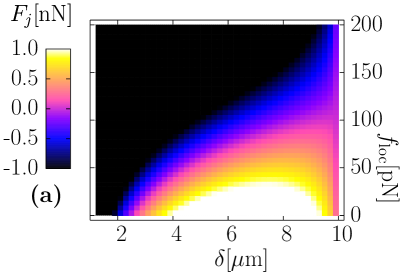
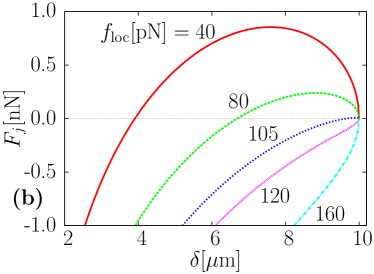
Figure 14: Force balancing in an isolated cell pair. The deterministic force $F_{j}=F_{ij}^{\text{(int)}}+F_{j}^{\text{(loc)}}$ acts on the cell center $\mathbf{x}_{j}$. Parameters are $f_{\text{int}}=60\,\mathrm{pN}$, $\alpha=1$, $r_{i}=3.0$, $r_{j}=2.0$, $\tilde{\rho}=6.6/\mathrm{\mu m}$, $\Delta_{\mathrm{min}}=0.2$, $\Delta_{\mathrm{crit}}=0.5$.

In figure 14 the resulting scalar horizontal force $F_{j}=F_{ij}^{\text{(int)}}+F_{j}^{\text{(loc)}}$ is plotted as a function of cell body distance $\delta$ and the locomotion force parameter $f_{\mathrm{loc}}$, revealing the emergence of a stable deterministic contact equilibrium $F_{j,\text{det}}=0$ for lower values of $f_{\mathrm{loc}}<105\,\mathrm{pN}$. On the other hand, for larger locomotion parameters, no such equilibrium exists and the cell distance always increases until the pair separates at $\delta=\delta_{ij}^{\mathrm{(rup)}}$ ($=10\mu\mathrm{m}$ in figure 14).

In order to study the full stochastic contact and segregation dynamics described by the SDE system (53) with noise amplitudes $\tilde{b}_{k}=b_{0}\sqrt{G_{k}(\phi_{k0}(\delta))}/\gamma_{k}$, $G_{k}(\phi)=|\Gamma_{k0}|=2\sqrt{\mathcal{P}_{\mathrm{max}}}r_{k}(\pi-\phi)$, we set all vertical noise components to zero, for simplicity. Then due to $F_{i}+F_{j}=0$ the dynamics is determined by differential equations for the cell overlap $z$ and the difference $u$ in horizontal cell velocities:

$$z=\delta_{ij}^{\mathrm{(rup)}}-\delta>0,\qquad u=v_{j}^{\text{(hor)}}-v_{i}^{\text{(hor)}}.$$ (55)

Proposition 2.

For cell pair dynamics restricted to the horizontal connection line the stochastic ODE system in equation (53) transforms into a nonlinear Ornstein-Uhlenbeck system for the overlap $z$ and its temporal change $u$, namely

$$\mathrm{d}z = u\,\mathrm{d}t$$ (56)

$$\mathrm{d}u = \Bigl{(}F(z)-u\Bigl{)}\frac{\mathrm{d}t}{T}+b(z)\cdot\mathrm{d}W_{t}$$ (57)

Defining the mean drag coefficient $1/\gamma_{ij}:=1/\gamma_{i}+1/\gamma_{j}$ and $C(\phi)$ as in equation (54), we have

$$F(z)=\frac{2\tilde{\rho}r_{j}}{\gamma_{ij}}\Bigl{(}f(z)C(\phi)-f_{\mathrm{loc}}\cdot\sin\phi\Bigr{)},\quad f(z)=f_{\mathrm{int}}\log\Bigl{(}\frac{z_{\mathrm{max}}-z}{z_{\mathrm{max}}-z_{c}}\Bigr{)},$$ (58)

$$b^{2}(z)=b_{0}^{2}\biggl{(}\frac{G_{j}(\phi)}{\gamma_{j}^{2}}+\frac{G_{i}(\phi)}{\gamma_{i}^{2}}\biggr{)},$$ (59)

with $z_{\mathrm{max}}=\delta_{ij}^{\mathrm{(rup)}}\cdot(1-\Delta_{\mathrm{min}})$ and $z_{c}=\delta_{ij}^{\mathrm{(rup)}}\cdot(1-\Delta_{\mathrm{crit}})$. The relation between $z=\delta_{ij}^{\mathrm{(rup)}}-\delta$ and $\phi=\phi_{j0}(\delta)$ can be written as

$$z\equiv R_{j0}\biggl{(}1-\sqrt{1-\sin^{2}\phi}\biggr{)}+R_{i0}\biggl{(}1-\sqrt{1-\eta^{2}\sin^{2}\phi}\biggr{)}.$$ (60)

Note that the overlap $z$ is a monotone function of $\sin\phi$, which is proportional to the vertical extension of the overlap region as spanned by the contact arc $\Gamma_{ij}$ (shaded in figure 7).

4.1 Asymptotic stochastic differential equations

Disruption of a connected pair occurs as $z\to 0$, so that an expansion at zero of all terms in Proposition 2 is justified. First, from equation (60) we derive the asymptotic relation

$$z=R_{j0}\frac{1+\eta}{2}\sin^{2}\phi\Bigl{(}1+\mathcal{O}\bigl{(}\sin^{2}\phi\bigr{)}\Bigr{)}$$

for $z>0$ so that

$$\phi\sim\sin\phi=\sqrt{\frac{2}{(1+\eta)R_{j0}}}\cdot\sqrt{z}\cdot\Bigl{(}1+\mathcal{O}(z)\Bigr{)}.$$

Thus, the locomotion term of the force $F(z)$ in equation (58) has a singularity at zero like $\sqrt{z}$. The same holds for the interaction term; as a surprise, the corresponding integral can be expanded in $\phi$ independent of the ratio $\eta=r_{j}/r_{i}$:

$$C(\varphi)=\int_{0}^{\phi}\mathrm{d}\varphi\,\Bigl{(}2-\varphi^{2}+\mathcal{O}\bigl{(}\varphi^{4}\bigr{)}\Bigr{)}=2\cdot\sin\phi\Bigl{(}1+\mathcal{O}\bigl{(}\phi^{4}\bigr{)}\Bigr{)}.$$

The conclusion is that the horizontal pair force can be approximated as

$$F(z)=2\frac{\tilde{\rho}r_{j}}{\gamma_{ij}}\sin\phi\biggl{(}2f(z)\Bigl{(}1+\mathcal{O}\bigl{(}z^{4}\bigr{)}\Bigr{)}-f_{\mathrm{loc}}\biggr{)},$$

where only the prefactor depends on the cell body sizes. The deterministic equilibrium overlap $z_{*}>0$, as the zero of $F$, is approximately determined by the force equality

$$f\bigl{(}z_{*}\bigr{)}=\frac{f_{\mathrm{loc}}}{2}\cdot\Bigl{(}1+\mathcal{O}\bigl{(}z_{*}^{2}\bigr{)}\Bigr{)}.$$

Thus, by using the definition of $f$ in equation (59), we define the contact parameter

$$\lambda:=z_{\mathrm{max}}-(z_{\mathrm{max}}-z_{c})\exp\biggl{(}\frac{f_{\mathrm{loc}}}{2f_{\mathrm{int}}}\biggr{)}.$$ (61)

Let us consider the deterministic overdamped dynamics $\dot{z}=F(z)$ obtained from the stochastic ODE system (56, 57) in the limit $T\to 0$. With $\gamma_{i}=\gamma_{j}=\tilde{\gamma}$ we prove the

Proposition 3 (Asymptotic contact and disrupture dynamics).

Given a pair of cells with body radii $r_{i}$ and $r_{j}$, with small contact parameter $|\lambda|$. Then there exists a unique stable equilibrium $z_{*}>0$ if and only if $\lambda>0$, namely $z_{*}=\lambda\bigl{(}1+\mathcal{O}(|\lambda|^{2})\bigr{)}>0$. Moreover, in the limit $T\to 0$, $\beta_{0}=b_{0}/\tilde{\gamma}T=\mathrm{const.}$, and the corresponding stochastic differential equation (SDE) can be approximately written as

$$\mathrm{d}z=\mu\sqrt{z_{+}}\ln\biggl{(}\frac{z_{\mathrm{max}}-z}{z_{\mathrm{max}}-\lambda}\biggr{)}\mathrm{d}t+\beta(z)\mathrm{d}W_{t}.$$ (62)

Here $z_{+}=\max(0,z)$ and

$$\mu=\tilde{\rho}\frac{G_{ij}}{2\tilde{\gamma}}\cdot f_{\mathrm{int}},\qquad\beta(z)=\beta_{0}\biggl{(}2\sqrt{\mathcal{P}_{\mathrm{max}}}\Bigl{(}(r_{i}+r_{j})\pi-G_{ij}\cdot\sqrt{z}\Bigr{)}\biggr{)}^{1/2},$$

with $G_{ij}=\bigl{(}8\sqrt{\mathcal{P}_{\mathrm{max}}}\cdot r_{i}r_{j}/(r_{i}+r_{j})\bigr{)}^{1/2}$.

Note that the $\log$ term in equation (62) can be approximated by $\bigl{(}\lambda-z+\mathcal{O}(z^{2})\bigr{)}/z_{\mathrm{max}}$, and $z^{*}=\lambda$ is a measure of the mean cell-cell overlap.

As soon as the contact between cells is lost, $z<0$, their cell center distance $d_{ij}=\sqrt{\mathcal{P}_{\mathrm{max}}}(r_{i}+r_{j})-z$ would perform a pure Brownian motion for $T=0$ or, for $T>0$, a persistent random walk with the standard recurrence probability to hit the touching state $z=0$ again. However, for situations of tissue cells moving on two-dimensional substrates, the production of adhesive fibers (as fibronectin) or remnants of plasma membrane plus adhesion molecules in the wake of a migrating cell would induce a positive bias of the locomotion force towards the other cell [27], which could be assumed as proportional to the cell boundary distance $-z$, at least for small distances. Therefore, and for the aim of exploring the resulting stationary process, instead of equations (62) we consider the extended SDE model

$$\mathrm{d}z=\tilde{F}(z)\mathrm{d}t+\beta(z)\mathrm{d}W_{t}$$ (63)

with

$$\tilde{F}(z)=\left\{\begin{aligned} &\mu\sqrt{z}\ln\biggl{(}\frac{z_{\mathrm{max}}-z}{z_{\mathrm{max}}-\lambda}\biggr{)}\quad&\text{for}\;z\geq 0\\ &-\nu z\quad&\text{for}\;z\leq 0\end{aligned}\right.$$

where we introduce an additional bias parameter $\nu>0$ describing an indirect attraction between separated cells.

4.2 Analysis of the stationary contact problem

By solving the stationary Kolmogorov forward equation, we compute the approximate stationary probability distribution for the overlap $z$ as

$$\begin{split}p(z)=&p_{0}\exp\biggl{(}\int_{0}^{z}\mathrm{d}z\;\frac{\tilde{F}(z)}{\beta^{2}(z)}\biggr{)}\\ =&\left\{\begin{aligned} &\frac{\mu}{\psi z_{\mathrm{max}}}z^{\frac{3}{2}}\Bigl{(}\frac{2}{3}\lambda+\frac{\lambda}{2\chi}z^{\frac{1}{2}}-\frac{2}{5}z\Bigr{)}\quad&\text{for}\;z\geq 0\\ &-\frac{\nu}{2\psi}|z|^{2}\quad&\text{for}\;z\leq 0\end{aligned}\right.\end{split}$$ (64)

with a unique normalization factor $p_{0}$ and additional lumped parameters that arise from expanding the singular noise variance $\beta^{2}(z)=2\psi\bigl{(}1-\sqrt{z(t)}/\chi+\mathcal{O}(z^{2}(t)\bigr{)}$:

$$\psi= \sqrt{\mathcal{P}_{\mathrm{max}}}\beta_{0}^{2}\pi(r_{i}+r_{j})^{2}$$

$$\chi^{2}= 8\pi^{2}\sqrt{\mathcal{P}_{\mathrm{max}}}(r_{i}+r_{j})^{2}\Bigl{(}\frac{1}{r_{i}}+\frac{1}{r_{j}}\Bigr{)}.$$

In figure 15(b) and (e), the probability distribution

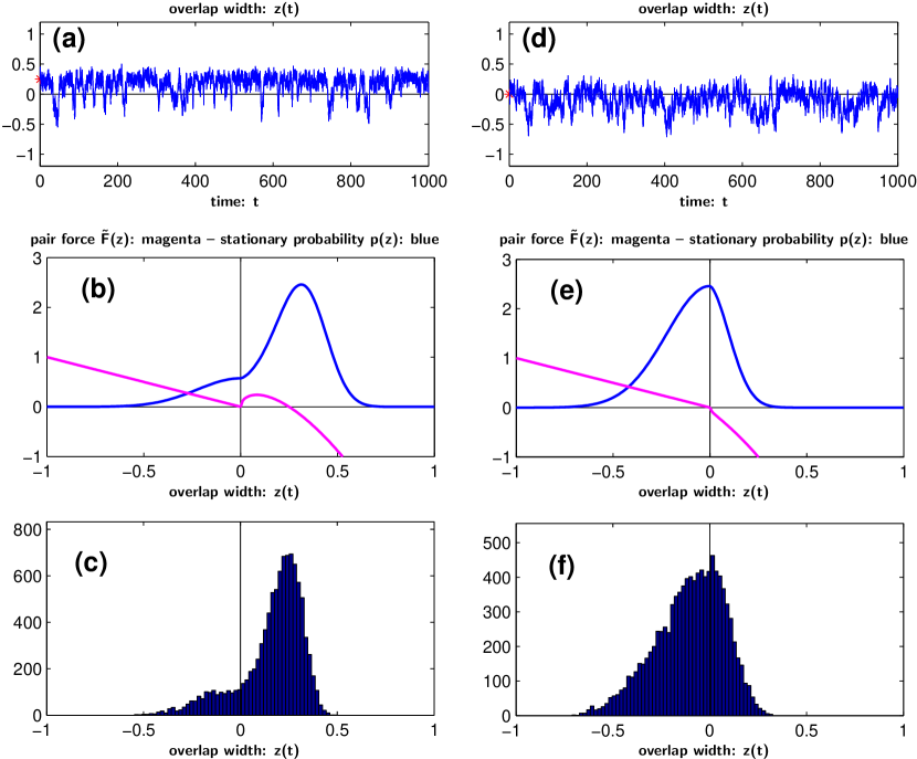
Figure 15: Analytical distribution (bold/blue in b,e), the corresponding simulation histograms (c,f), and the time series (a,d) of the overlap width $z$. This quantity emerges from the dynamics of equation (63) for contact parameter $\lambda>0$ (a-c) and $\lambda<0$ (d-f), respectively, with force $\tilde{F}(z)$ (grey/magenta in b,e). Time $t$ is given in units of min, overlap $z$ in units of $\mu\mathrm{m}$, and force $F$ in $\mathrm{nN}$. Parameters used are $\beta_{0}=0.1$, $\psi=\beta_{0}^{2}$, $z_{\mathrm{max}}=0.1$ and $z_{c}=0.5$.

$p(z)$ according to equation (64) is plotted for two special parameter sets together with the force function $\tilde{F}(z)$, whereas in figure 15(c) and (f) histograms for the corresponding numerical realizations of the stochastic differential equation (63) are shown. For the contact parameter $\lambda=0.25>0$, see definition 61, there appears a skew-shaped modified Gauss distribution around the unique center $z_{*}=\lambda$ with a certain probability $P_{\text{off}}=\int_{-\infty}^{0}\mathrm{d}z\,p(z)\approx 0.15$ for the cells to be separated. In contrast, for $\lambda=-0.15<0$, the standard Gauss distribution with variance $\psi/\nu$ for positive separation distances $-z$ is cut off by a decreasing distribution of the positive overlap $z$ with mean value $Z_{\text{cont}}=\int_{0}^{\infty}\mathrm{d}z\,zp(z)\approx 0.08\ll z_{*}$ and a certain contact probability $P_{\text{cont}}=1-P_{\text{off}}\approx 0.32$.

Figure 16 shows the plot of the separation probability $P_{\text{off}}$ over

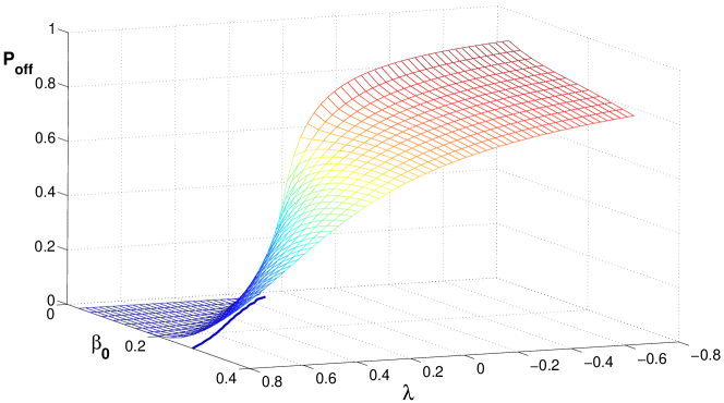
Figure 16: Separation probability $P_{\text{off}}=\int_{-\infty}^{0}\mathrm{d}z\,p(z)$ according to (64) plotted over the parameter plane of contact ($\lambda$) and noise ($\beta_{0}$). In this plane the contour curve $P_{\text{off}}=0.05$ is drawn in blue. The other parameters are the same as in figure 15. More details are given in the text.

the contact and noise parameters $\lambda$ and $\beta_{0}$ together with the contour curve for the critical value $\lambda_{0.05}=\lambda(\beta_{0})$, so that the separation probability $P_{\text{off}}$ is less than $5\%$ for contact parameters $\lambda>\lambda_{0.05}$, i.e. for

$$\frac{2f_{\mathrm{int}}}{f_{\mathrm{loc}}}>\log\biggl{(}\frac{\Delta_{\mathrm{crit}}-\Delta_{\mathrm{min}}}{1-\Delta_{\mathrm{min}}-\lambda_{0.05}/\delta_{ij}^{\mathrm{(rup)}}}\biggr{)}.$$

For the two cases of contact parameters $\lambda>0$ and $\lambda<0$, the corresponding time series of the overlap distance $z$ as plotted in figure 15(a) and (d), respectively, reveal a clearly distinct temporal separation and contact behavior.

In the first case, with lower locomotion force parameter $f_{\mathrm{loc}}$ relative to the interaction parameter $f_{\mathrm{int}}$, the contact state persists for longer time intervals. Thereby, the overlap fluctuates around the equilibrium value $z_{*}=\lambda$, with mean contact duration $\tau_{\text{cont}}\approx\exp(2.8)\,\text{min}\approx 16\,\text{min}$. This proper contact time is evaluated from the maximum of the right-side $\tau$-hump in the logarithmic histogram of figure 17(a).

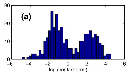
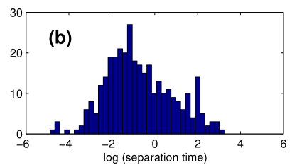
Figure 17: Logarithmically scaled duration histogram of contact intervals (a) and separation intervals (b) for a longer time series ($3000\,\text{min}$) of the situation in figure 15(a).

.

The contact states are interrupted by periods of faster flickering, as can be seen from the change between on and off with a mean duration of $\tau_{\text{flicker}}\approx\exp(-1.5)\approx 15\mathrm{s}$, which is visible at the joint lower maximum in both figures 17(a) and (b). Otherwise, an intermediate separation of the order of 1-5 min occurs.

Yet for the second case, $\lambda<0$, with relatively higher locomotion force parameter $f_{\mathrm{loc}}$, we observe in figure 15(d) dominating periods of flickering around the steady state of touching $z_{*}=0$, which now is a stable deterministic equilibrium, even super-stable for $z>0$ with convergence $z(t)\sim(t_{*}-t)^{2/3}$ in finite time. Longer periods of separation are also evident but their distribution does not differ much from the situation for $\lambda>0$ (similar to the histogram in figure 17(b), not shown here).

5 Tissue simulations

After these analytic considerations in the case of cell pair formation we return to the full equations of motion (53). Since both time and length scale of cell motility processes are well known, the only remaining free scaling figure is the magnitude of cell forces. In accordance to [4], here we assume that a typical bundle of several actin filaments can exert a force of approximately $10\,\mathrm{pN}$. A single cell can, with the overall filament density parameter $\tilde{\rho}$ and the force prefactors $f_{\mathrm{loc}},f_{\mathrm{int}}$ as in table 1, reach an effective traction of $\mathcal{O}(1000\,\mathrm{pN})$

$\sqrt{\mathcal{P}_{\mathrm{max}}}=3$	$\tilde{\rho}=9.55/\mu\mathrm{m}$	$\tilde{\gamma}=2.5\cdot 10^{4}\,\mathrm{pN\,s}/\mu\mathrm{m}$
$\mathrm{d}t=2\,\mathrm{s}$	$\Delta_{\mathrm{min}}=0.1$	$f_{\mathrm{int}}=60\,\mathrm{pN}$
$T=120\,\mathrm{s}$	$\Delta_{\mathrm{crit}}=0.2\dots 0.7$	$f_{\mathrm{loc}}=10\dots 20\,\mathrm{pN}$
$b_{0}\cdot(\mathcal{P}_{\mathrm{max}})^{1/4}=8.31\,\mathrm{pN}/\sqrt{\mu\mathrm{m}\,\mathrm{s}}$		$\alpha=0\dots 0.17$

Table 1: Simulation and model parameters as described previously. Unless indicated otherwise, all simulations have been performed with this parameter set.

from a force as given by equation (44). The drag coefficient $\tilde{\gamma}$ then naturally follows from experimentally observed cell velocities [50, 20, 33]. As explained before, $T$ is the persistence time of the intracellular cytoskeletal reorganization, and $\mathcal{P}_{\mathrm{max}}$ determines the relative size of the lamella region around the cell body $\mathcal{B}_{r_{i}}(\mathbf{x}_{i})$. Moreover, the scaled interaction distances $\Delta_{\mathrm{min}},\Delta_{\mathrm{crit}}$ as defined in equation (42) determine the sign and scaling of the cell pair interaction force $\mathbf{F}_{ij}^{\mathrm{(int)}}$. The relative strength of the vertical component of $\mathbf{F}_{ij}^{\mathrm{(int)}}$ in equation (43) is given by $\alpha$. Finally, the stochastic perturbation parameter $b_{0}$ in equation (50) contains a factor $(\mathcal{P}_{\mathrm{max}})^{-1/4}$ in order to obtain the same amount of perturbation for cells with equal body radii $r_{i}$. Since we look for robust features in the simulations, $b_{0}$ was chosen fairly high.

5.1 Emergence of tissue shape and multiple stable states

Consider a simple proto-tissue of seven cells as shown in

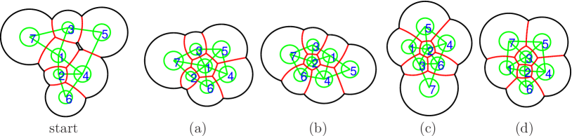
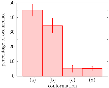
Figure 18: Different tissue conformations (a-d) evolving from the configuration ‘start’ after a simulation time of $8\,\mathrm{h}$; here $r_{\text{max}}=2.0\,\mu\mathrm{m}$ (cell $7$), $r_{\text{min}}=1.0\,\mu\mathrm{m}$ (cell $2$), and parameters $f_{\mathrm{loc}}=20\,\mathrm{pN},\;\alpha=0,\;\Delta_{\mathrm{crit}}=0.25$. The percentage of occurrence of a particular conformation then was computed, and the error bars were obtained by a simple bootstrap method. Other features are further explained in the text.

figure 18 ‘start’. Using the parameters $f_{\mathrm{loc}}=20\,\mathrm{pN},\alpha=0,\Delta_{\mathrm{crit}}=0.25$, a series of $1000$ simulations has been performed. After a simulation time of $8\mathrm{h}$, the emerging tissue conformations as distinguished by Delaunay network topology have been recorded. In the course of these $8\mathrm{h}$, significant changes appear within the tissue, and apparently several equilibrium conformations emerge. For the four most prevalent conformations the percentage of occurrence is displayed in figure 18. One observes two rather globular shapes (a), (d), where either the big cell $1$ or the two small cells $2,3$ are engulfed by the others, respectively. Furthermore, there are two more elongated shapes (b), (c), where only the single small cell $2$ is completely surrounded by other cells. Being distinguished by topology, (b) and (c) are in fact quite close in shape, despite of their rotational variation.

From the high occurrence of the topological conformations (a), (b) one might conclude that these two conformations are the most stable ones. Thus, and to clarify the interrelations between the conformations (a-d), we investigate (a) and (b) in longer simulations. To this end, by starting from the configurations (a) and (b) (see figure 18), both tissues have been evolved for $40$ additional hours of simulation time. In order to characterize the shape of tissue with respect to global and elongated shape, here we observe tissue size, i.e. the maximum diameter, and tissue circularity

$$\Omega=\frac{2\sqrt{\pi A_{\text{tiss}}}}{\sum_{i}|\Gamma_{i0}|}\leq 1,$$

where $A_{\text{tiss}}$ is the total area of the tissue. Note that in connected tissues $\Omega=1$ would be attained for a purely circular globe. Other observables are possible but less indicative in this context.

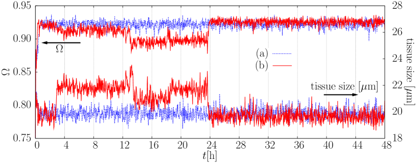
Figure 19: Two time series (blue, red) for the tissue in figure 18 ‘start’. After $8\,\mathrm{h}$ the two distinct topological conformations from figure 18(a) (blue) and 18(b) (red) have emerged. These topological conformations are characterized by distinct tissue size (right axis) and circularity $\Omega$ (left axis). While (a) is apparently a stable topological conformation that does not change even for strong stochastic perturbations, (b) relaxes into a topological conformation of globular shape via several intermediate steps, see supplementary mova.avi, movb.avi.

In figure 19, the two time series (blue, red) soon reach the different conformations of figure 18(a) and (b) respectively, at times around $t\sim 8\mathrm{h}$. While the circularity $\Omega$ is only slightly different in the two cases, the tissue size is clearly higher for the elongated conformation (b). Apart from stochastic fluctuations and an initial equilibration phase for $t<1\,\mathrm{h}$, both observables attain a constant value for time series (a). In contrast, for time series (b) there appear distinct states between $t\sim 2.5\,\mathrm{h}$ and $t\sim 24\,\mathrm{h}$. Indeed these observations are reflected by the actual evolution of the tissue. While the topology of the tissue does not change after $t=2\,\mathrm{h}$ for time series (a) (see supplementary mova.avi), tissue (b) (movb.avi) goes through several different conformational states. At $t=13.5\,\mathrm{h}$ it attains the same topology as conformation (c), identifying (c) as a transient state (movc.avi). Afterwards, approximately at $t\sim 18.5\,\mathrm{h}$, cell $7$ establishes contact with cells $1,3$, so that the tissue shape is similar to (c). Finally, shortly before $t=24\,\mathrm{h}$, the tissue reaches its final conformation similar to (d) except for the order of the marginal cells. Conformation (d) emerges in a similar manner as (a), however instead of cells $1,5$ initially cells $3,4$ form a neighbor pair, quickly leading to the stable final arrangement in less than $0.5\,\mathrm{h}$ (see supplementary movd.avi). Moreover, the time series of conformation (b) in figure 19 suggests, that during $t=0.5\dots 3\,\mathrm{h}$ the tissue already attains a shape of similar compactness and stability as in figure 18(a). Nevertheless, the Delaunay mesh (green lines) is not convex there (movb.avi), which explains this surprising instability.

It appears, that the stability of a tissue is related to its globular shape. This is not a surprise, since the stochastic forces in equation (48) are defined only on free cell boundaries $\Gamma_{i0}$, and therefore act only on marginal cells. Thus, by minimizing the extent of all $\Gamma_{i0}$, a maximal circularity minimizes stochastic perturbations, which enhances the stability of the tissue. Additionally, for a tissue to change its topology, its cells have to overcome barriers as imposed by the other cells. For example, cell $3$ has to displace cell $1$ in movb.avi at $t\approx 3\,\mathrm{h}$ in order to make contact with $2$. Depending on the particular configuration, the severity of these barriers might range from prohibitive to practically non-existent. Influenced by the strength of the stochastic interactions, these barriers then determine the time scale of further relaxation to equilibrium. In this sense, the notion of equilibrium is directly related to an inherent time scale. According to the previous evolution of the tissue, there may be several stable topological conformations for a given time scale.

5.2 Stability of tissue formation

In order to explore the ramifications of piecewise spherical cells within our model framework, we study the influence of $\mathcal{P}_{\mathrm{max}}$ and $\Delta_{\mathrm{crit}}$ on tissue formation. To this end, a simulation has been performed starting from an exemplary configuration as in figure 6 with $\Delta_{\mathrm{crit}}=0.3,\sqrt{\mathcal{P}_{\mathrm{max}}}=3,\alpha=0.17$ and $f_{\mathrm{loc}}=10\,\mathrm{pN}$. After $8\,\mathrm{h}$, either $\Delta_{\mathrm{crit}}$ or $\sqrt{\mathcal{P}_{\mathrm{max}}}$ was modified to a nearby parameter position as indicated in figure 20,

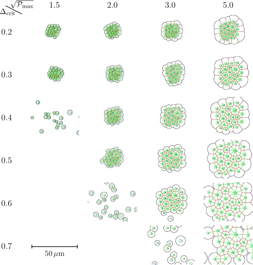
Figure 20: Stability of tissue for various values of the parameters $\sqrt{\mathcal{P}_{\mathrm{max}}}$ and $\Delta_{\mathrm{crit}}$, where $f_{\mathrm{loc}}=10\,\mathrm{pN}$, and $\alpha=0.17$. When increased, both parameters lead to an increased tissue size. For sufficiently large $\Delta_{\mathrm{crit}}$, the tissue eventually dissociates. The extremal cell body radii are $r_{\mathrm{min}}=0.9\,\mu\mathrm{m}$ and $r_{\mathrm{max}}=1.7\,\mu\mathrm{m}$ in all simulations presented in this figure.

and the simulation was continued for further $8\,\mathrm{h}$. This procedure was repeated until the whole panel in 20 was filled with the final tissue configurations.

For fixed $\{r_{i}\}$, the overall size of the tissue is determined by both $\sqrt{\mathcal{P}_{\mathrm{max}}}$, defining the free cell radius $R_{i0}$ in units of $r_{i}$, and $\Delta_{\mathrm{crit}}$, presetting the equilibrium cell-cell body distance in units of $\delta_{ij}^{\mathrm{(rup)}}$, see equations (21), (42) and (40). Correspondingly, in figure 20, the overall tissue extension increases from left to right and from top to bottom. Furthermore, for given $\Delta_{\mathrm{crit}}$, tissues with higher $\sqrt{\mathcal{P}_{\mathrm{max}}}$ exhibit a rather compact, almost quadratic shape. We speculate that this is due to spontaneous formation of distinct protrusions arising from stochastic perturbations and leading to an increase of locomotion at the corners. In contrast, tissues with lower $\sqrt{\mathcal{P}_{\mathrm{max}}}$ feature more irregular margins. Similarly, for given $\sqrt{\mathcal{P}_{\mathrm{max}}}$, larger values of $\Delta_{\mathrm{crit}}$ yield more irregularity, most pronounced directly before dissociation of the tissue.

Apparently, the emerging interaction forces are sufficiently strong for tissue aggregation only if there is enough space for the adaptation of neighboring cell lamellae. This space serves as a cushion for accommodating near-range repulsion from multiple neighbor cells and at the same time poses a resistance to stochastic perturbations by mid-range neighbor cell attraction, see figure 14. Otherwise the tissue dissociates, leading to isolated cells exclusively driven by stochastic perturbations. In order to quantify these findings, consider the relative lamella width $\mathcal{W}$ and the dimensionless cell overlap $\mathcal{Z}$ defined by

$$\mathcal{W}=\frac{\sqrt{\mathcal{P}_{\mathrm{max}}}-1}{\sqrt{\mathcal{P}_{\mathrm{max}}}}<1,\qquad\qquad\mathcal{Z}=1-\Delta_{\mathrm{crit}}<1.$$

Inserting the marginal values $\sqrt{\mathcal{P}_{\mathrm{max}}}$ and $\Delta_{\mathrm{crit}}$ of those tissues in figure 20 that are not yet dissociated, one recognizes that the product $\mathcal{Z}\cdot\mathcal{W}=:\mathcal{T}_{0}$ is approximately constant, with $\mathcal{T}_{0}\approx 0.24$,

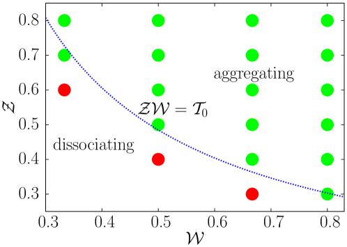
Figure 21: Tissue aggregation and dissociation depending on the relative lamella width $\mathcal{W}$ and the dimensionless cell overlap $\mathcal{Z}$. The line $\mathcal{Z}\cdot\mathcal{W}=\mathcal{T}_{0}\approx 0.24\pm 3\%$ separates associating from dissociating tissues and was determined from a linear regression against $\mathcal{Z}=\mathcal{T}_{0}/\mathcal{W}$. See also the explanations in the text.

see figure 21. This $\mathcal{T}_{0}$ can be identified as a threshold value guaranteeing tissue coherence under the condition

$$\mathcal{Z}\cdot\mathcal{W}\geq\mathcal{T}_{0},$$ (65)

where $\mathcal{T}_{0}$ eventually depends on the other parameters, which were fixed here. This confirms that for tissue aggregation to occur, $\sqrt{\mathcal{P}_{\mathrm{max}}}$ and with it the relative lamella width $\mathcal{W}$ must be sufficiently large.

On the other hand, we have established this result under the tissue homogeneity condition (46) guaranteeing starlikeness of cells, which now can be rewritten as

$$\mathcal{Z}_{\text{max}}\cdot\mathcal{W}=1-\frac{1}{Q_{\mathrm{nb}}},$$ (66)

with $\mathcal{Z}_{\text{max}}:=1-\Delta_{\mathrm{min}}$ defining the maximal dimensionless overlap. Since $\mathcal{W}<1$ by construction, inequality (66) always holds for very high cell size homogeneities $Q_{\mathrm{nb}}\geq 1/\Delta_{\mathrm{min}}$. However, for lower $Q_{\mathrm{nb}}$ there is an upper bound on $\mathcal{W}$ restricting the available space for the cell lamellae. If, in addition, starlikeness of cells is enforced for all possible neighborhood constellations, then $Q_{\mathrm{nb}}$ has to be replaced by $Q$, see equation (24). In this way the relations (65) and (66) lead to the sufficient condition for tissue coherence

$$\frac{\mathcal{T}_{0}}{1-\Delta_{\mathrm{crit}}}\leq\mathcal{W}=1-\frac{1}{\sqrt{\mathcal{P}_{\mathrm{max}}}}\leq\frac{2}{(1-\Delta_{\mathrm{min}})(1+r_{\text{max}}/r_{\text{min}})}.$$ (67)

From these estimates we finally conclude that for given model force parameters ($\Delta_{\mathrm{min}}$, $\Delta_{\mathrm{crit}}$, $f_{\mathrm{int}}$, $\alpha$, $f_{\mathrm{loc}}$, $b_{0}$) the formation of integer tissue aggregates with overall starlike cells is guaranteed within a certain finite range of the free cell size parameter $\sqrt{\mathcal{P}_{\mathrm{max}}}$, where the upper bound decreases with an increasing ratio $r_{\text{max}}/r_{\text{min}}$ of extremal cell body radii. Within the limits of inequality (67) the lamellae regions are wide enough to perform the necessary deformations by adapting to the surrounding neighbors through shape changes. Thus, nature’s freedom in developing aggregating tissues may be constrained by a tradeoff between the relative size of cells with respect to their bodies ($\sqrt{\mathcal{P}_{\mathrm{max}}}$) and the cell size heterogeneity ($1/Q$).

6 Results and discussion

In this article we have investigated the emergence of tissue aggregation using finite, generalized Voronoi neighborhoods as a basis for the description of cells within epithelial tissues. It was shown that the two-dimensional geometric structure observed in tissues, in particular the circular shape of contact arcs and the size distribution of cells can be captured by the experimentally accessible characteristics of cell body radii $\{r_{i}\}$ and the relative extension $\mathcal{P}_{\mathrm{max}}$ of the lamellae. The quotient method defined by equation (17) with unique weight factors $w_{i}=r_{i}$ implements the expected partition of influence regions and additionally suggests the definition of directed force densities on the contact and free boundaries. In contrast, the difference method is not appropriate, because the influence region of a cell growing in size becomes reduced within a cell pair. Nevertheless this method has been used previously for modelling three-dimensional tissue dynamics [35, 37]. By using the particular additive weights $w_{i}=r_{i}$, the specific geometrical properties (“orthocircles”) allow for a dense regular triangulation of space between neighboring cell bodies even in the case of overlap, see [10] for details.

In the asymptotic case of two cells in brief contact, i.e. $\delta_{ij}\approx\delta_{ij}^{\mathrm{(rup)}}$, the approximate equations of overdamped motion without persistence were treated analytically. Thereby, the contact singularity at the rupture points could be resolved and a stationary probability distribution was found under the assumption that separated cells indirectly attract each other due to biased locomotion. Corresponding simulations confirm that in the case of dominating attraction, i.e. contact parameter $\lambda>0$, there is indeed a unique, stable equilibrium position facilitating cell-cell attachment after the first contact.

The simulations of multicellular dynamics, cf. figure 20, reveal a surprising richness of tissue structure, with emerging shapes from elongated to globular and from compact quadratic to irregular and dispersed. Ranging from widely spread to tightly contracted, different lamella protrusions appear for varying $\mathcal{P}_{\mathrm{max}}$. Similarly, within a more or less compressed tissue as in figure 6, single cells attain varying forms from almost circular at the margins to polygonal in the interior. Moreover, distinct stresses throughout the tissue lead to both narrowly compressed or widely stretched cell shapes.

Furthermore, due to the stochastic nature of neighbor constellation and cell-cell interactions, different stable tissue configurations may evolve from the same starting configuration. The underlying dynamical time scales vary over several orders of magnitude. This can be interpreted in terms of an incomplete balance of competing interactions within a system. In the course of relaxation to equilibrium, this is known to cause frustration, meaning that the system ends up in a local minimum of the involved (generalized) free energy [38, 34, 26]. Thus, the structure of the proposed anisotropic and active force interactions exhibits interesting non-trivial features, yet it is sufficiently elementary to allow for a rigorous treatment under certain further assumptions.

Finally, the limits of aggregation due to a prohibitively small tissue coherence threshold $\mathcal{T}_{0}$ have been explored. This leads to our main result following from purely geometric arguments: In proposition 1 we have derived that relatively large lamellae extensions $\mathcal{P}_{\mathrm{max}}$ are restricted by the cell size homogeneity $Q_{\mathrm{nb}}$ when requiring starlikeness of cells. On biological grounds one might argue that not all observed cells are starlike (in the mathematical sense). In such a case, however, the exertion of forces onto neighboring cells is certainly hindered – especially in cell regions that cannot be reached by radial filaments. There, the necessary centro-radial support of the apical actin cortex may be weakened due to the necessary bending of filament bundles. Reversing the argument, for the cell to provide macroscopic stability within the tissue, it is beneficial to attain a starlike shape.

Several model refinements are of interest. On the cell biological side, cell division is a commonly observed phenomenon, having special consequences for pattern formation and self-organization during embryonic development. In this direction also the growth of cells, or even the complete cell cycle including necrosis or apoptosis could be considered. On the mathematical side more elaborate stochastics, such as differentially modeled stochastic forces on the free boundaries as well as on the contact borders could be implemented. In particular, in the light of recent experimental results [40, 29], varying filament orientations or binding and unbinding processes of linker molecules might be considered. Moreover, we emphasize that a three-dimensional generalization of the multiplicatively weighted Voronoi tessellation is straight-forward, opening a wide potential for applications, for example epidermal tissue organization in the intestinal crypt without artificially imposed constraints. Finally, explicit variables for cell polarization and reorganization of the cytoskeleton could possibly lead to refined dynamics closer resembling the behavior observed in vivo.

Acknowledgements: We thank D. Bär, G. Schaller and M. Meyer-Hermann for helpful discussions, and G. Wenzel and G. Kirfel for providing us with microscopic pictures. This work was supported by the Deutsche Forschungsgemeinschaft, SFB 611 “Singular Phenomena and Scaling in Mathematical Models”.

References

- [1] B. Alberts, A. Johnson, J. Lewis, K. Roberts, and P. Walter, editors. Molecular Biology of the Cell. Garland Science, 4th edition, 2002. Chapters 16 and 19.
- [2] H.-W. Alt and W. Alt. Phase boundary dynamics: Transitions between ordered and disordered lipid monolayers. Interfaces and Free Boundaries, 11:1, 2009.
- [3] W. Alt. Nonlinear hyperbolic systems of generalized Navier-Stokes type for interactive motion in biology. In: S. Hildebrandt and H. Karcher, editors, Geometric Analysis and Nonlinear Partial Differential Equations, page 431. Springer, 2003.
- [4] R. Ananthakrishnan and A. Ehrlicher. The forces behind cell movement. International Journal of Biological Sciences, 3:303, 2007.
- [5] L. Arnold. Stochastic differential equations: theory and applications. Wiley Interscience, 1974.
- [6] P. Ash and E. Bolker. Generalized Dirichlet tessellations. Geometrica Dedicata, 20:209, 1986.
- [7] F. Aurenhammer and H. Edelsbrunner. An optimal algorithm for constructing the weighted Voronoi diagram in the plane. Pattern Recognition, 17:251, 1984.
- [8] F. Aurenhammer and R. Klein. Voronoi Diagrams. Technical Report 198, FernUniversität Hagen, 1996. http://wwwpi6.fernuni-hagen.de/Publikationen/tr198.pdf.
- [9] J. Bernal. Bibliographic notes on Voronoi diagrams. Technical Report 5164, U.S. Dept. of Commerce, National Institute of Standards and Technology, 1993. ftp://math.nist.gov/pub/bernal/or.ps.Z.
- [10] T. Beyer and M. Meyer-Hermann. Modeling emergent tissue organization involving high-speed migrating cells in a flow equilibrium. Physical Review E, 76:021929, 2007.
- [11] T. Beyer, G. Schaller, A. Deutsch, and M. Meyer-Hermann. Parallel dynamic and kinetic regular triangulation in three dimensions. Computer Physics Communications, 172:86, 2005.
- [12] J. Brevier, D. Montero, T. Svitkina, and D. Riveline. The asymmetric self-assembly mechanism of adherens junctions: A cellular push–pull unit. Physical Biology, 5:016005, 2008.
- [13] L. Brillouin. Les électrons dans les métaux et le classement des ondes de de Broglie correspondantes. Comptes Rendus Hebdomadaires des Séances de l’Académie des Sciences, 191:292, 1930.
- [14] W. Brodland and J. Veldhuis. Computer simulations of mitosis and interdependencies between mitosis orientation, cell shape and epithelia reshaping. Journal of Biomechanics, 35:673, 2002.
- [15] P. Dieterich, J. Seebach, and H. Schnittler. Quantification of shear stress-induced cell migration in endothelial cultures. In: A. Deutsch, M. Falcke, J. Howard and W. Zimmermann, editors, Function and Regulation of Cellular Systems: Experiments and Models, Mathematics and Biosciences in Interaction, page 199. Birkhäuser, 2004.
- [16] G.L. Dirichlet. Über die Reduction der positiven quadratischen Formen mit drei unbestimmten ganzen Zahlen. Journal für Reine und Angewandte Mathematik, 40:209, 1850.
- [17] D. Drasdo and G. Forgacs. Modeling the interplay of generic and genetic mechanisms in cleavage, blastulation, and gastrulation. Developmental Dynamics, 219:182, 2000.
- [18] D. Drasdo, R. Kree, and J.S. McCaskill. Monte Carlo approach to tissue-cell populations. Physical Review E, 52:6635, 1995.
- [19] E. Evans and K. Ritchie. Dynamic strength of molecular adhesion bonds. Biophysical Journal, 72:1541, 1997.
- [20] P. Friedl, K.S. Zänker, and E.-B. Bröcker. Cell migration strategies in 3-D extracellular matrix: Differences in morphology, cell matrix interactions and integrin function. Microscopy Research and Technique, 43:369, 1998.
- [21] J. Galle, M. Loeffler, and D. Drasdo. Modeling the effect of deregulated proliferation and apoptosis on the growth dynamics of epithelial cell populations in vitro. Biophysical Journal, 88:62, 2005.
- [22] Y. Gambin, R. Lopez-Esparza, M. Reffay, E. Sierecki, N.S. Gov, M. Genest, R.S. Hodges, and W. Urbach. Lateral mobility of proteins in liquid membranes revisited. Proceedings of the National Academy of Sciences, USA, 103:2098, 2006.
- [23] Y. Hegerfeldt, M. Tusch, E.-B. Bröcker, and P. Friedl. Collective cell movement in primary melanoma explants: Plasticity of cell-cell interaction, -integrin function and migration strategies. Cancer Research, 62:2125, 2002.
- [24] H. Honda. Description of cellular patterns by Dirichlet domains: The two-dimensional case. Journal of Theoretical Biology, 72:523, 1978.
- [25] H. Honda, M. Tanemura, and T. Nagai. A three-dimensional vertex dynamics cell model of space-filling polyhedra simulating cell behavior in a cell aggregate. Journal of Theoretical Biology, 226:439, 2004.
- [26] W. Janke, editor. Rugged Free Energy Landscapes: Common Computational Approaches to Spin Glasses, Structural Glasses and Biological Macromolecules, volume 736 of Lecture Notes in Physics. Springer, Berlin, 2008.
- [27] G. Kirfel, A. Rigort, B. Borm, C. Schulte, and V. Herzog. Structural and compositional analysis of the keratinocyte migration track. Cell Motility and the Cytoskeleton, 55:1, 2003.
- [28] P.E. Kloeden, E. Platen. Numerical solution of stochastic differential equations. Springer, 1992. Chapter 8.
- [29] S.A. Koestler, S. Auinger, M. Vinzenz, K. Rottner, and J.V. Small. Differentially oriented populations of actin filaments generated in lamellipodia collaborate in pushing and pausing at the cell front. Nature Cell Biology, 10:306, 2008.
- [30] E. Kuusela and W. Alt. Continuum model of cell adhesion and migration. Journal of Mathematical Biology, 58:135, 2009.
- [31] H. Marie, S.J. Pratt, M. Betson, H. Epple, J.T. Kittler, L. Meek, S.J. Moss, S. Troyanovsky, D. Attwell, G.D. Longmore, and V.M. Braga. The LIM protein Ajuba is recruited to cadherin-dependent cell junctions through an association with alpha-catenin. Journal of Biological Chemistry, 278:1220, 2003.
- [32] F. Meineke, S. Potten, and M. Loeffler. Cell migration and organization in the intestinal crypt using a lattice-free model. Cell Proliferation, 34:253, 2001.
- [33] C. Möhl. Modellierung von Adhäsions- und Cytoskelett-Dynamik in Lamellipodien migratorischer Zellen. Diploma thesis, Universität Bonn, 2005.
- [34] E.H. Purnomo, D. van den Ende, S.A. Vanapalli, and F. Mugele. Glass transition and aging in dense suspensions of thermosensitive microgel particles. Physical Review Letters, 101:238301, 2008.
- [35] G. Schaller. On selected numerical approaches to cellular tissue. PhD thesis, Johann Wolfgang Goethe-Universität, Frankfurt am Main, 2005.
- [36] G. Schaller and M. Meyer-Hermann. Kinetic and dynamic Delaunay tetrahedralizations in three dimensions. Computer Physics Communications, 162:9, 2004.
- [37] G. Schaller and M. Meyer-Hermann. Multicellular tumor spheroid in an off-lattice Voronoi-Delaunay cell model. Physical Review E, 71:051910, 2005.
- [38] C. Semmrich, T. Storz, J. Glaser, R. Merkel, A.R. Bausch, and K. Kroy. Glass transition and rheological redundancy in F-actin solutions. Proceedings of the National Academy of Sciences, USA, 104:20199, 2007.
- [39] M. Shamos and D. Hoey. Closest point problems. In Proceedings of the 16th Annual IEEE Symposium on Foundations of Computer Science (FOCS), page 151, 1975.
- [40] S. Sivaramakrishnan, J.V. DeGuilio, L. Lorand, R.D. Goldman, and K.M. Ridge. Micromechanical properties of keratin intermediate filament networks. Proceedings of the National Academy of Sciences, USA, 105:889, 2008.
- [41] D. Sulsky, S. Childress, and J.K. Percus. A model for cell sorting. Journal of Theoretical Biology, 106:275, 1984.
- [42] K.M. Taute, F. Pampaloni, E. Frey, and E.-L. Florin. Microtubule dynamics depart from the wormlike chain model. Physical Review Letters, 100:028102, 2008.
- [43] A.H. Thiessen. Precipitation averages for large areas. Monthly Weather Reviev, 39:1082, 1911.
- [44] C.L. Tinkle, A. Pasolli, N. Stokes, and E. Fuchs. New insights into cadherin function in epidermal sheet formation and maintenance of tissue integrity. Proceedings of the National Academy of Sciences, USA, 105:15405, 2008.
- [45] G. Voronoi. Nouvelles applications des paramètres continus à la théorie de formes quadratiques. Journal für die Reine und Angewandte Mathematik, 134:198, 1908.
- [46] M. Weliky, S. Minsuk, R. Keller, and G. Oster. Notochord morphogenesis in Xenopus laevis: Simulation of cell behavior underlying tissue convergence and extension. Development, 113:1231, 1991.
- [47] M. Weliky and G. Oster. The mechanical basis of cell rearrangement. I. Epithelial morphogenesis during Fundulus epiboly. Development, 109:373, 1990.
- [48] E. Wigner and F. Seitz. On the constitution of metallic sodium. Physical Review, 43:804, 1933.
- [49] B. Young and J.W. Heath, editors. Wheater’s Functional Histology: A Text and Colour Atlas. Churchill Livingstone, 2000.
- [50] J.-M. Zahm, H. Kaplan, A.-L. Hérard, F. Doriot, D. Pierrot, P. Somelette, and E. Puchelle. Cell migration and proliferation during the in vitro wound repair of the respiratory epithelium. Cell Motility and the Cytoskeleton, 37:33, 1997.