On the phase diagram of the Higgs model
Abstract:
The Higgs model with (fixed Higgs length) is usually believed to have two different phases at high gauge coupling , separated by a line of first order transitions but not distinuguished by any typical symmetry associated with a local order parameter, as first proved by Fradkin and Shenker. We show that in regions of the parameter space where it is usually supposed to be a first order phase transition only a smooth crossover is in fact present.
1 Introduction and motivation
While in pure gauge theories there is a standard way to detect color confinement (the Wilson criterium [1]), when matter in the fundamental representation of the gauge group is present, large Wilson loops never obey the area-law, so that there is no obvious way to clearly define the meaning of “confined phase”.
From the computational point of view, the simplest such model is the Higgs model; to study only the general features of its phase diagram, this model can be simplified a bit more, fixing the length of the Higgs field. This is possible because the scalar fourth-coupling is irrelevant in continuum limit and fixing the length of the Higgs field is equivalent to use (the irrelevance of was numerically checked in [2]). In this case the action can be written in the form (see e.g. [2])
| (1) |
where the first term is the standard Wilson action and the Higgs field is written using an matrix. This form of the action is particularly useful because with it standard heatbath ([3], [4]) and overrelaxation ([5]) algorithms can be used to generate Monte Carlo configurations.
A theory with action 1 has the following important limiting cases
-
: pure gauge theory, no transitions in
-
: non linear sigma model, it has a second order phase transition in
The general case was studied in [6] using both perturbative and non-peturbative methods: using a pertubative expansion it was shown that the transition of the model is not lifted out by the introduction of the gauge field, but it becames a first order à la Coleman-Weinberg. On the non-perturbative side, using the methods developed in [7], the authors of [6] were able to prove the existence of a wide region of parameter space where every local observable is analytic, the so called Fradkin Shenker (FS) theorem. Using these two inputs they suggested a phase diagram like that shown in Fig. 1: the region where the analyticity is rigorously proven is indicated by AR and is limited by the dotted line, the thick line represents a line of first order transitions and the two dots are its second order end-points.
Since the FS theorem ensures that no local observable can be used in all the parameter space to discriminate between a “confined phase” and a “Higgs phase”, there are some efforts to analyze the behaviour in this model of the most popular proposals for confinement order parameter and to study how the (possible) singularities in these operators are related to the first order transition line of the thermodynamical observables (see e.g. [8], [9]). Because of that it is useful to have a precise location of the line of first order transitions and of its critical end-point, which is absent in the literature on the model.
2 Results of simulations
The first numerical results on the Higgs model appeared in [10] and seemed to display the features of the phase diagram in Fig. 1, but they were obtained on a very small lattice, so that further study was needed to confirm it. Subsequently, in [11], the existence of a double peak structure was claimed at on a lattice, strongly supporting the first order scenario; however this was probably just a consequence of the poor statistics, since in [12] no double peak was observed at and “the system exhibits a transient behavior up to along which the order of the transition cannot be discerned”. To improve these results we analyzed the points and , on lattices up to , looking for a clear first order transition. The observables monitored are
-
•
the gauge-Higgs coupling,
-
•
the plaquettes,
-
•
the monopoles, , where stand for the elementary cube and
-
•
the Polyakov loops
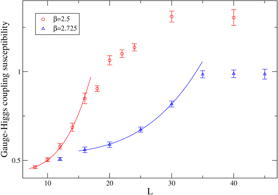
Among the observables, the most sensitive one turned out to be the gauge-Higgs coupling, whose susceptibility peak heights and Binder fourth order cumulant minima are shown in Fig. 2 and 3. The susceptibility of the operator is defined in the ususal way, , while the Binder fourth order cumulant is ; if in the thermodynamic limit a discontinuity in is present at , the susceptibility develops maxima whose heigth scale as , while has minima whose asymptotic behaviour is (see e.g. [13])
| (2) |
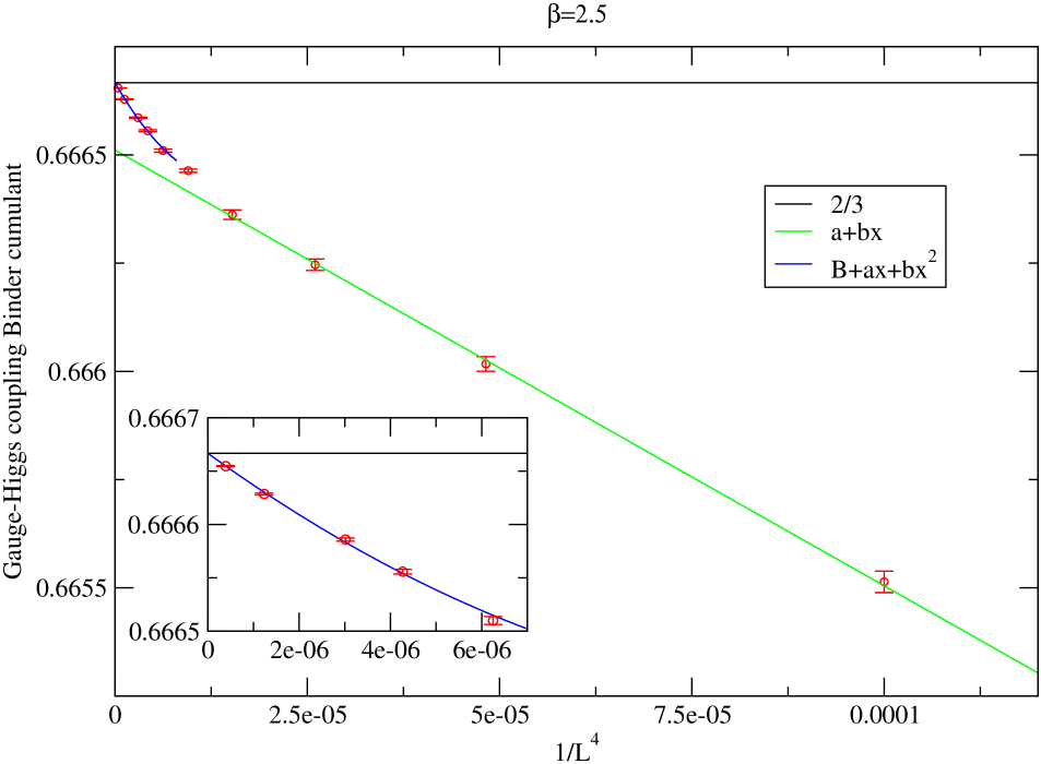
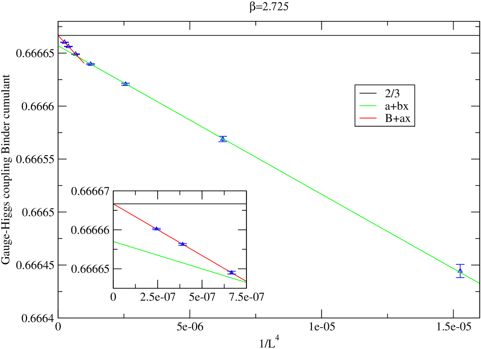
so that for a first-order transition is less than . As is clear from Fig. 2 and 3, both susceptibility and Binder cumulant have two different typical behaviours depending on the lattice size: for small lattices they have a first order-like scaling, while for larger lattices cross-over nature of the system appears. Indeed for lattice sizes with and lattice sizes with the susceptibilities are well described by the function (Fig. 2) and Binder cumulants do not seem to reach (Fig. 3); only going to larger lattices it is possible to see the susceptibility saturate and the Binder fourth order cumulant tend to : the values of the costant obteined from the fits shown in the magnifications in Fig. 3 are and for and respectively.
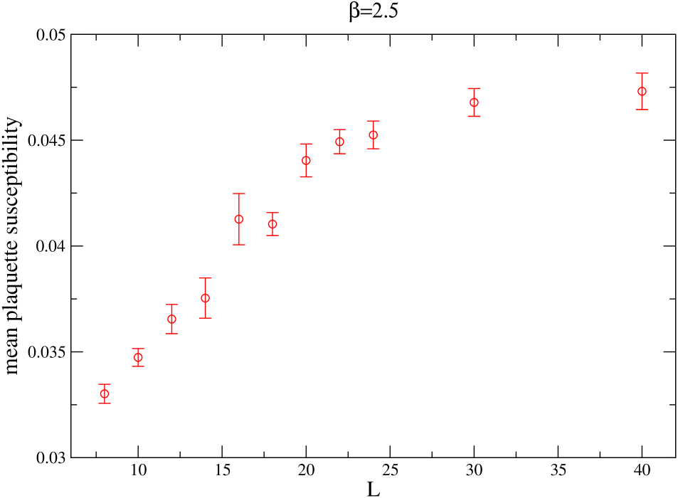
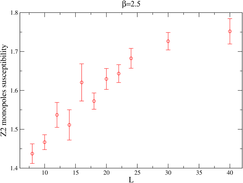
A similar type of behaviour is seen also in the susceptibilities of all the other observables, like the mean plaquette and the monopole (Fig. 4) as well as in the way Polyakov loop reaches its asymptotic value. In Fig. 5 the Polyakov loop value is shown for fixed and and for various : the red line is the result of a fit to using only data ( and ) while the green one is obteinded using only ( and ); in both cases because of the Higgs field, however is clear that an extrapolation making use only of small volumes would be badly wrong.
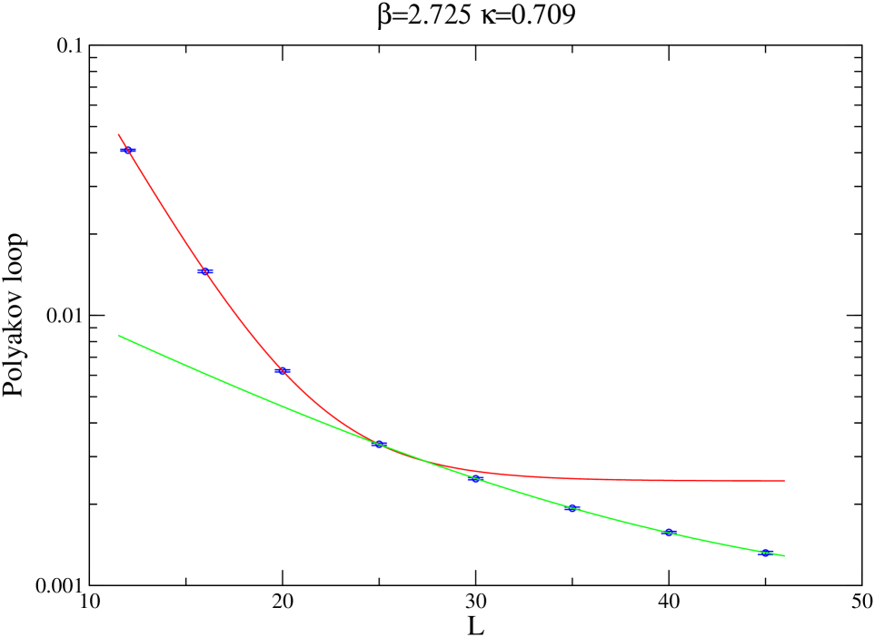
The presence in all the observables of two different behaviours at small and big volumes is not at all new in lattice gauge theories, since to a finite cubic lattice corresponds a finite temperature, so that a deconfinement transition is to be expected for some value of the parameters; the new features are the possbility to describe the small volumes regime to high precision using a first-order scaling and the surprisingly big lattice dimensions needed to reveal the true thermodynamical properties of the model.
3 Conclusions
We performed simulations at and , where a first order transition is usually believed to exist, and we found that all the analysed observables have instead smooth infinite volume limits; we thus conclude that in this region only a smooth cross-over is present. Moreover we discovered that in order to see the correct non-singular behaviour it is necessary to use lattices much bigger than the ones typically adopted in studies of the Higgs model.
At this stage it is not possible to predict whether the end-point exists at or the line of first-order transition is in fact absent; in order to clarify this point it would be necessary either to study even greater values (but before a nonperturbative analysis of the -function is needed to ensure the lattice spacing is big enough) or to keep track of the end-point positions at increalsing (at the existence of the first-order line was verified in [14]) and try to extrapolate it to the limit.
References
- [1] K.G.Wilson Confinement of quarks. Phys. Rev. D 10, 2445 (1974).
- [2] I.Montvay Correlations and static energies in the standard Higgs model. Nucl. Phys. B 269, 170 (1986).
- [3] M.Creutz Monte Carlo study of quantized gauge theory. Phys. Rev. D 21, 2308 (1980).
- [4] A.D.Kennedy, B.J.Pendleton Improved heatbath method for Monte Carlo calculations in lattice gauge theories. Phys. Lett. B 156, 393 (1985).
- [5] M.Creutz Overrelaxation and Monte Carlo simulation. Phys. Rev. D 36, 515 (1987).
- [6] E. Fradkin, S.H.Shenker Phase diagrams of lattice gauge theories with Higgs fields. Phys. Rev. D 19, 3682 (1979).
- [7] K.Osterwalder, E.Seiler Gauge Field Theories on a Lattice. Ann. Phys. 110, 440 (1978).
- [8] J. Greensite, Š, Olejník Vortices, symmetry breaking, and temporary confinement in gauge-Higgs theory. Phys. Rev. D 74, 014502 (2006) (hep-lat/0603024).
- [9] W.Caudy, J.Greensite On the ambiguity of spontaneously broken gauge symmetry, Phys. Rev. D 78, 025018 (2008) (arXiv:0712.0999 [hep-lat]).
- [10] C.B.Lang, C.Rebbi, M.Virasoro The phase structure of a non-abelian gauge Higgs field system. Phys. Lett. B 104, 294 (1981).
- [11] W.Langguth, I.Montvay Two-state signal at the deconfinement-Higgs phase transition in the standard Higgs model. Phys. Lett. B 165, 135 (1985).
- [12] I.Campos On the -Higgs phase transition. Nucl. Phys. B 514, 336 (1998) (hep-lat/9706020).
- [13] J.Lee, J.M.Kosterlitz Finite-size scaling and Monte Carlo siulations of first-order phase trasitions. Phys. Rev. B 43, 3265 (1991).
- [14] W.Bock et alt. Search for critical points in the Higgs model. Phys. Rev. D 41, 2573 (1990).