On the phenomenology of a two-Higgs-doublet model with maximal CP symmetry at the LHC

Abstract

Predictions for LHC physics are worked out for a two-Higgs-doublet model having four generalized CP symmetries. In this maximally-CP-symmetric model (MCPM) the first fermion family is, at tree level, uncoupled to the Higgs fields and thus massless. The second and third fermion families have a very symmetric coupling to the Higgs fields. But through the electroweak symmetry breaking a large mass hierarchy is generated between these fermion families. Thus, the fermion mass spectrum of the model presents a rough approximation to what is observed in Nature. In the MCPM there are, as in every two-Higgs-doublet model, five physical Higgs bosons, three neutral ones and a charged pair. In the MCPM the couplings of the Higgs bosons to the fermions are completely fixed. This allows us to present clear predictions for the production at the LHC and for the decays of the physical Higgs bosons. As salient feature we find rather large cross sections for Higgs-boson production via Drell–Yan type processes. With experiments at the LHC it should be possible to check these predictions.

1 Introduction

The Standard Model (SM) of particle physics is very successful in describing the currently known experimental data; see Amsler:2008zz for a review. Nevertheless, the SM leaves open a number of theoretical questions. Thus, various extensions of the SM have been studied extensively. With the start-up of the LHC we can hope that experiments will soon give decisive answers in which way - if at all - the SM has to be extended; see Ellis:2007vz for a brief overview of these topics.

In this paper we shall study a particular two-Higgs-doublet model (THDM) and develop its LHC phenomenology. The model, which we want to call maximally-CP-symmetric model (MCPM) for reasons which will become clear later, has the field content as in the SM except for the Higgs sector, where we have two Higgs doublets instead of only one. Many versions of THDMs have been studied in the literature; see Kobayashi:1973fv ; Gunion:1989we ; Cvetic:1993cy ; Ginzburg:2004vp ; Gunion:2005ja ; Barbieri:2005kf ; Branco:2005em ; Nishi:2006tg ; Barbieri:2006dq ; Ivanov:2006yq ; Fromme:2006cm ; Ivanov:2007de ; Barroso:2007rr ; Gerard:2007kn and references therein. In our group we have studied various aspects of the most general THDM in Maniatis:2006fs ; Maniatis:2007vn . A class of interesting models having a maximal number of generalized CP symmetries was found. In Maniatis:2007de these models were studied in detail and it was shown that the requirement of maximal CP invariance led to a very interesting structure for the coupling of fermions to the Higgs fields. Maximal CP invariance requires more than one fermion family if fermions are to get non-zero masses. With the additional requirement of absence of flavor-changing neutral currents at tree level and of mass-degenerate massive fermions a unique Lagrangian was derived. This Lagrangian is very symmetric between the second and third fermion families before electroweak symmetry breaking (EWSB) occurs. But after EWSB the third family becomes massive, the second family stays massless. In this model also the first family is massless and the Cabibbo–Kobayashi–Maskawa (CKM) matrix equals the unit matrix. Of course, all this is not exactly as observed in Nature. But, on the other hand, it may be a starting point to understand some aspects of the large fermion mass hierarchies observed experimentally.

In the present paper we shall work out concrete predictions for LHC physics which follow from the two-Higgs-doublet model with maximal CP invariance, the MCPM, having the large fermion mass hierarchies as discussed in Maniatis:2007de . In Sect. 2 we recall the main features of the Lagrangian. In Sect. 3 we give our predictions for the decays of the physical Higgs particles of the MCPM. Section 4 deals with Higgs-boson production at the LHC. We draw our conclusions in Sect. 5. In Appendix A we give the explicit form of the Lagrangian and some Feynman rules of the MCPM. If the MCPM, in the strict symmetry limit, represents not too bad an approximation to the real world then this should also be true for its LHC phenomenology as discussed in this paper. Thus, our work should be considered as presenting the generic features of this phenomenology.

2 The model

A detailed study of the MCPM can be found in Ref. Maniatis:2007de . Here we want to recall the motivation and the essential steps to construct this model.

The general gauge-invariant and renormalizable potential $V(\varphi_{1},\varphi_{2})$ of the two Higgs doublets $\varphi_{1}$ and $\varphi_{2}$ is a hermitian linear combination of the terms

$$\varphi_{i}^{\dagger}\varphi_{j},\quad(\varphi_{i}^{\dagger}\varphi_{j})(\varphi_{k}^{\dagger}\varphi_{l})\;,$$ (1)

with $i,j,k,l\in\{1,2\}$. The $SU(2)_{L}\times U(1)_{Y}$ invariant scalar products are arranged into the hermitian, positive semi definite, $2\times 2$ matrix

$$\underline{K}(x):=\begin{pmatrix}\varphi_{1}^{\dagger}\varphi_{1}&\varphi_{2}^{\dagger}\varphi_{1}\\ \varphi_{1}^{\dagger}\varphi_{2}&\varphi_{2}^{\dagger}\varphi_{2}\end{pmatrix}\,.$$ (2)

Its decomposition reads

$$\underline{K}(x)=\frac{1}{2}\left(K_{0}(x)\mathbbm{1}_{2}+\boldsymbol{\mathrm{K}}(x)\,\boldsymbol{\mathrm{\sigma}}\right)$$ (3)

with Pauli matrices $\sigma^{a}\ (a=1,2,3)$. In this way one defines the real gauge-invariant functions

$$K_{0} =\varphi_{1}^{\dagger}\varphi_{1}+\varphi_{2}^{\dagger}\varphi_{2}, K_{1} =2\operatorname{Re}\varphi_{1}^{\dagger}\varphi_{2},$$ (4)

$$K_{3} =\varphi_{1}^{\dagger}\varphi_{1}-\varphi_{2}^{\dagger}\varphi_{2}, K_{2} =2\operatorname{Im}\varphi_{1}^{\dagger}\varphi_{2}\,.$$

In terms of these functions the general THDM potential can be written in the simple form

$$V= \;\xi_{0}\,K_{0}(x)+\boldsymbol{\mathrm{\xi}}^{\mathrm{T}}\,\boldsymbol{\mathrm{K}}(x)+\eta_{00}\,K_{0}^{2}(x)$$

$$+2\,K_{0}(x)\,\boldsymbol{\mathrm{\eta}}^{\mathrm{T}}\,\boldsymbol{\mathrm{K}}(x)+\boldsymbol{\mathrm{K}}^{\mathrm{T}}(x)\,E\,\boldsymbol{\mathrm{K}}(x)\,,$$ (5)

with $\boldsymbol{\mathrm{K}}=(K_{1},K_{2},K_{3})^{\mathrm{T}}$ and parameters $\xi_{0}$, $\eta_{00}$, three-component vectors $\boldsymbol{\mathrm{\xi}}$, $\boldsymbol{\mathrm{\eta}}$ and the $3\times 3$ matrix $E=E^{\mathrm{T}}$. All parameters in (2) are real.

One now proceeds to study CP transformations in the general THDM. Writing the Higgs potential in the form (2) one finds a simple geometric picture for CP transformations. The standard CP transformation ($\mathrm{CP_{s}}$) of the Higgs doublets is

$$\varphi_{i}(x)\xrightarrow{\mathrm{CP_{s}}}\phantom{-}\varphi_{i}^{*}(x^{\prime})\,,\qquad(i=1,2)\,,$$ (6)

where, due to the parity transformation $x^{\prime}=(x_{0},-\boldsymbol{\mathrm{x}})^{\mathrm{T}}$. In terms of the gauge invariant functions, this $\mathrm{CP_{s}}$ transformation is simply $K_{0}(x)\rightarrow K_{0}(x^{\prime})$ and

$$\begin{split}K_{1}(x)&\rightarrow\phantom{-}K_{1}(x^{\prime})\;,\\ K_{2}(x)&\rightarrow-K_{2}(x^{\prime})\;,\\ K_{3}(x)&\rightarrow\phantom{-}K_{3}(x^{\prime})\;.\end{split}$$ (7)

Geometrically, this is a reflection on the 1–3 plane in $\boldsymbol{\mathrm{K}}$ space in addition to the argument change. Motivated by this geometric picture, generalized CP transformations ($\text{CP}_{g}$) corresponding to reflections on planes ($\text{CP}_{g}^{(ii)}$) as well as to the point reflection ($\mathrm{CP}_{g}^{(i)}$) in $\boldsymbol{\mathrm{K}}$ space were studied in Maniatis:2007vn ; Maniatis:2007de . The $\mathrm{CP}_{g}^{(i)}$ transformation is given by $K_{0}(x)\rightarrow K_{0}(x^{\prime})$ and

$$\boldsymbol{\mathrm{K}}(x)\rightarrow-\boldsymbol{\mathrm{K}}(x^{\prime})$$ (8)

and plays a central role in the construction of the MCPM. In Maniatis:2007de some distinguishing features of this transformation are discussed. In terms of the original Higgs doublets these $\text{CP}_{g}$ transformations read generically

$$\varphi_{i}(x)\rightarrow W_{ij}\varphi^{\ast}_{j}(x^{\prime})\,.$$ (9)

The $2\times 2$ matrices $W$ corresponding to the transformations $\mathrm{CP}_{g}^{(i)}$ and to $\text{CP}_{g,a}^{(ii)}$ ($a=1,2,3$), the reflections on the coordinate planes in $\boldsymbol{\mathrm{K}}$ space, are given in the second row of Tab. 1, where we defined

$$\epsilon=\begin{pmatrix}\phantom{+}0&\phantom{+}1\\ -1&\phantom{+}0\end{pmatrix}\;.$$ (10)

The transformation $\text{CP}_{g,2}^{(ii)}$ is, of course, just $\mathrm{CP_{s}}$ given in (6), (7). For $\text{CP}_{g,1}^{(ii)}$ ($\text{CP}_{g,3}^{(ii)}$) the transformation of the $\boldsymbol{\mathrm{K}}$ vector is similar to (7) but with the sign change for $K_{1}$ ($K_{3}$).

$\text{CP}_{g}$		$\;\;W\;\;$	$\;\;U_{R}\;\;$	$\;\;U_{L}\;\;$
point reflection	$\mathrm{CP}_{g}^{(i)}$	$\epsilon$	$\phantom{+}\epsilon$	$\sigma^{1}$
2–3 plane reflection	$\text{CP}_{g,1}^{(ii)}$	$\sigma^{3}$	$-\sigma^{3}$	$\mathbbm{1}_{2}$
1–3 plane reflection	$\text{CP}_{g,2}^{(ii)}$	$\mathbbm{1}_{2}$	$\phantom{+}\mathbbm{1}_{2}$	$\mathbbm{1}_{2}$
1–2 plane reflection	$\text{CP}_{g,3}^{(ii)}$	$\sigma^{1}$	$-\sigma^{1}$	$\sigma^{1}$

Table 1: The matrices $W$ of (9) and $U_{L}$ and $U_{R}$ of (2) for the four generalized CP invariances.

Now we are in a position to recall the construction principles of the MCPM, that is, a THDM which respects all generalized CP symmetries of Tab. 1. We start with the THDM Higgs potential (2). Requiring it to be symmetric under the generalized CP transformation $\mathrm{CP}_{g}^{(i)}$ leads with a suitable basis choice to

$$V(\varphi_{1},\varphi_{2})=\xi_{0}K_{0}+\eta_{00}K_{0}^{2}+\mu_{1}K_{1}^{2}+\mu_{2}K_{2}^{2}+\mu_{3}K_{3}^{2}\;.$$ (11)

Note that here $K_{a}$, ($a=1,2,3$) enter only quadratically. This implies that the potential $V$ of (11) is also invariant under the transformation $\mathrm{CP_{s}}\equiv\text{CP}_{g,2}^{(ii)}$ which just changes the sign of the component $K_{2}$; see (7). Similarly one finds invariance of $V$ (11) under $\text{CP}_{g,1}^{(ii)}$ and $\text{CP}_{g,3}^{(ii)}$. Thus, the potential is invariant under the point reflection symmetry (8) as well as all three different reflections on the coordinate planes in $\boldsymbol{\mathrm{K}}$ space. In this way the Higgs potential of the MCPM is determined.

The next step is to extend these $\text{CP}_{g}$ symmetries to the Yukawa terms, which couple the fermions $\psi(x)$ to the Higgs doublets. We define the generalized CP transformations of the fermions generically as

$$\text{CP}_{g}\,:\quad \psi_{\alpha\,L}(x) \rightarrow U_{L\,\alpha\beta}\,\gamma^{0}\,S(C)\,\bar{\psi}_{\beta\,L}^{\mathrm{T}}(x^{\prime})\,,$$

$$\psi_{\alpha\,R}(x) \rightarrow U_{R\,\alpha\beta}\,\gamma^{0}\,S(C)\,\bar{\psi}_{\beta\,R}^{\mathrm{T}}(x^{\prime})$$ (12)

with family indices $\alpha$, $\beta$, $S(C)=i\gamma^{2}\gamma^{0}$ the usual matrix of charge conjugation, and unitary matrices $U_{L}$ and $U_{R}$. As shown in the detailed study Maniatis:2007de having only one family coupled to the Higgs bosons in a $\mathrm{CP}_{g}^{(i)}$-symmetric way leads necessarily to vanishing Yukawa couplings, that is, to massless fermions. Thus, in the MCPM two families are coupled via Yukawa terms to the Higgs doublets. By convention these families are given the indices two and three. One finds that the Yukawa interactions are highly restricted requiring them to be invariant under the generalized CP transformations of Tab. 1 for the fermions (2) and Higgs doublets (9). Moreover, the Yukawa couplings are uniquely defined, if in addition to these $\text{CP}_{g}$ invariances one requires non-degenerate fermion masses and absence of large flavor-changing neutral currents (FCNCs). The corresponding matrices $U_{L}$ and $U_{R}$ are presented in the last two rows in Tab. 1. Eventually, one ends up with the Yukawa part of the Lagrangian of the MCPM in the form

$$\mathscr{L}_{\mathrm{Yuk}}(x)=-c^{(1)}_{l\,3} \;\Bigg{\{}\bar{\tau}_{R}(x)\,\varphi_{1}^{\dagger}(x)\begin{pmatrix}\nu_{\tau\,L}(x)\\ \tau_{L}(x)\end{pmatrix}$$

$$-\bar{\mu}_{R}(x)\,\varphi_{2}^{\dagger}(x)\begin{pmatrix}\nu_{\mu\,L}(x)\\ \mu_{L}(x)\end{pmatrix}\Bigg{\}}$$

$$+c^{(1)}_{u\,3} \;\Bigg{\{}\bar{t}_{R}(x)\,\varphi_{1}^{\mathrm{T}}(x)\,\epsilon\begin{pmatrix}t_{L}(x)\\ b_{L}(x)\end{pmatrix}$$

$$-\bar{c}_{R}(x)\,\varphi_{2}^{\mathrm{T}}(x)\,\epsilon\begin{pmatrix}c_{L}(x)\\ s_{L}(x)\end{pmatrix}\Bigg{\}}$$

$$-c^{(1)}_{d\,3} \;\Bigg{\{}\bar{b}_{R}(x)\,\varphi_{1}^{\dagger}(x)\begin{pmatrix}t_{L}(x)\\ b_{L}(x)\end{pmatrix}$$

$$-\bar{s}_{R}(x)\,\varphi_{2}^{\dagger}(x)\begin{pmatrix}c_{L}(x)\\ s_{L}(x)\end{pmatrix}\Bigg{\}}+h.c.$$ (13)

where $c^{(1)}_{l\,3}$, $c^{(1)}_{u\,3}$ and $c^{(1)}_{d\,3}$ are real positive constants, determined by the fermion masses as discussed below. The first family remains uncoupled – at tree level – to the Higgs bosons in the MCPM.

Now we come to the questions of stability and EWSB in the MCPM. As discussed in Maniatis:2007vn ; Maniatis:2007de the MCPM is stable, produces the correct breaking $SU(2)_{L}\times U(1)_{Y}\rightarrow U(1)_{\mathrm{em}}$, and has no zero mass or mass degenerate Higgs bosons if and only if the parameters of $V$ in (11) satisfy

$$\mu_{1}>\mu_{2}>\mu_{3}\;,$$

$$\eta_{00}>0\;,$$

$$\mu_{a}+\eta_{00}>0,\quad{\text{for }}a=1,2,3\;,$$ (14)

$$\xi_{0}<0\;,$$

$$\mu_{3}<0\;.$$

Through EWSB only the Higgs doublet $\varphi_{1}$ gets a vacuum expectation value (VEV). In the unitary gauge we have

$$\varphi_{1}(x)=\frac{1}{\sqrt{2}}\begin{pmatrix}0\\ v_{0}+\rho^{\prime}(x)\end{pmatrix}\;,$$ (15)

$$\varphi_{2}(x)=\begin{pmatrix}H^{+}(x)\\ \frac{1}{\sqrt{2}}(h^{\prime}(x)+ih^{\prime\prime}(x))\end{pmatrix}\;,$$ (16)

where $\rho^{\prime}(x)$, $h^{\prime}(x)$ and $h^{\prime\prime}(x)$ are the real fields corresponding to the physical neutral Higgs particles. The fields $H^{+}(x)$ and $H^{-}(x)=\big{(}H^{+}(x)\big{)}^{\ast}$ correspond to the physical charged Higgs pair. In (15) $v_{0}$ is the standard VEV

$$v_{0}\approx 246\text{ GeV}\;,$$ (17)

which is given in terms of the original potential parameters of (11) by

$$v_{0}=\sqrt{\frac{-\xi_{0}}{\eta_{00}+\mu_{3}}}\;.$$ (18)

Inserting (15) and (16) into (4) and (11) it is straightforward to calculate the masses of the physical Higgs fields in terms of the original parameters

$$\begin{split}m_{\rho^{\prime}}^{2}\;\;&=2(-\xi_{0})\;,\\ m_{h^{\prime}}^{2}\;\;&=2v_{0}^{2}(\mu_{1}-\mu_{3})\;,\\ m_{h^{\prime\prime}}^{2}\;&=2v_{0}^{2}(\mu_{2}-\mu_{3})\;,\\ m_{H^{\pm}}^{2}&=2v_{0}^{2}(-\mu_{3})\;.\end{split}$$ (19)

Conversely, one can express the original parameters $\xi_{0},...,\mu_{3}$ by $v_{0}$ and the Higgs-boson masses

$$\begin{split}\xi_{0}&=-\frac{1}{2}m_{\rho^{\prime}}^{2}\;,\\ \eta_{00}&=\frac{1}{2v_{0}^{2}}(m_{H^{\pm}}^{2}+m_{\rho^{\prime}}^{2})\;,\\ \mu_{1}&=\frac{1}{2v_{0}^{2}}(m_{h^{\prime}}^{2}-m_{H^{\pm}}^{2})\;,\\ \mu_{2}&=\frac{1}{2v_{0}^{2}}(m_{h^{\prime\prime}}^{2}-m_{H^{\pm}}^{2})\;,\\ \mu_{3}&=-\frac{1}{2v_{0}^{2}}m_{H^{\pm}}^{2}\;.\end{split}$$ (20)

The stability and correct $SU(2)_{L}\times U(1)_{Y}$ symmetry breaking conditions (14) require positive squared masses and

$$m_{h^{\prime}}^{2}>m_{h^{\prime\prime}}^{2}\;.$$ (21)

Thus, (21) is the only strict relation for the Higgs-boson masses which one gets in the MCPM. On the other hand, if we require that the Higgs sector has weak couplings only, we should have $\eta_{00}$, $|\mu_{1}|$, $|\mu_{2}|$ and $|\mu_{3}|$ to be less than or equal to a number of ${\cal O}(1)$. From (19) we expect then that the masses of $h^{\prime}$, $h^{\prime\prime}$ and $H^{\pm}$ should be less than about $2v_{0}\approx 500$ GeV. But by no means should this be considered as a necessary upper bound for the Higgs-boson masses in the MCPM.

Upon EWSB the Yukawa term (2) produces masses for the charged fermions of the third family. Inserting (15) and (16) into (2) gives

$$\begin{split}m_{\tau}&=c^{(1)}_{l\,3}\frac{v_{0}}{\sqrt{2}}\;,\\ m_{t}&=c^{(1)}_{u\,3}\frac{v_{0}}{\sqrt{2}}\;,\\ m_{b}&=c^{(1)}_{d\,3}\frac{v_{0}}{\sqrt{2}}\;.\end{split}$$ (22)

The fermions of the second and the first families stay massless in the fully-symmetric theory at tree level. Of course, this is only an approximation valid for the tree-level investigations. Fortunately, from the numerical studies which follow below, we will see that the main features of the LHC phenomenology of the MCPM are insensitive to the first- and second-family masses due to their smallness.

The next task is to express the Lagrangian of the MCPM in terms of the physical fields in the unitary gauge. This is done in Appendix A. From there the Feynman rules of the MCPM can be read off. In Appendix A we give these rules for the three-point vertices which are relevant for us in the following. Some salient features are as follows.

• The neutral Higgs boson $\rho^{\prime}$ couples to the third-family fermions as the physical Higgs boson $\rho^{\prime}_{SM}$ of the SM.

• The neutral Higgs boson $h^{\prime}$ has a scalar coupling to the second-family fermions. The Higgs boson $h^{\prime\prime}$ which is lighter than $h^{\prime}$ has a pseudoscalar coupling to the second-family fermions. But the coupling constants for $h^{\prime}$ and $h^{\prime\prime}$ are proportional to the masses of the third-family fermions, that is, to $m_{\tau}$, $m_{t}$ and $m_{b}$.

• Also the charged Higgs bosons $H^{\pm}$ couple only to the second-family fermions but again with coupling constants proportional to the masses of the third-family fermions.

As we shall see in the following these features lead to quite distinct phenomenological predictions of the MCPM for LHC physics.

We summarize this section. We have recalled the construction principles of the model which has the four generalized CP symmetries of Tab. 1. As can easily be seen from (11) this is the maximal number of such symmetries, including $\mathrm{CP}_{g}^{(i)}$, one can have in a THDM if one requires absence of zero mass and mass degenerate physical Higgs bosons. Thus, the name maximally–CP–symmetric model, MCPM, seems justified. The extension of the four generalized CP symmetries to the Yukawa interaction gave drastic restrictions for the family structure of the model and led, finally, with some additional arguments to the coupling (2). The remaining sections of this paper are devoted to discussing physical consequences of the MCPM.

3 Higgs-boson decays

The decays of the Higgs particles of the MCPM which are possible at tree level can be directly read off from the Lagrangian in the form given in (A.5) of Appendix A. We have decays of a Higgs particle into a fermion and an antifermion, and of a Higgs particle into another Higgs particle plus a gauge boson $W$ or $Z$. Furthermore, we could have decays of one Higgs boson into two other Higgs bosons and one Higgs boson into another Higgs boson plus two gauge bosons if the mass differences of the various Higgs bosons are large enough. In the following we shall restrict ourselves to discussing the tree-level results for the fermionic and the Higgs boson plus gauge boson decays and the results for the loop-induced two-photon and two-gluon decays.

3.1 Fermionic decays

The generic fermionic decay of a Higgs particle $H_{1}$ is

$$H_{1}(k)\rightarrow f^{\prime}(p_{1})+\bar{f}(p_{2})$$ (23)

where $f$ and $f^{\prime}$ denote the fermions and the momenta are indicated in brackets. The corresponding diagram and analytic expression at tree level for the vertex are shown in Fig. 1. The possible decays together with the corresponding coupling constants $a$ and $b$ are listed in Tab. 2. There, $N_{c}^{f}$ is the color factor which equals $1$ for leptons and $3$ for quarks. The decay rate for the generic decay (23) is calculated as

$$\Gamma(H_{1}\rightarrow f^{\prime}+\bar{f})=\\ \frac{N_{c}^{f}}{8\pi v_{0}^{2}}\frac{w(m_{H_{1}}^{2},m_{f}^{2},m_{f^{\prime}}^{2})}{m_{H_{1}}^{2}}\;m_{H_{1}}\;\theta(m_{H_{1}}-m_{f}-m_{f^{\prime}})\\ \bigg{\{}|a|^{2}+|b|^{2}-\frac{(m_{f}+m_{f^{\prime}})^{2}}{m_{H_{1}}^{2}}|a|^{2}-\frac{(m_{f}-m_{f^{\prime}})^{2}}{m_{H_{1}}^{2}}|b|^{2}\bigg{\}}\;.$$ (24)

$-i\frac{1}{v_{0}}(a+b\;\gamma_{5})$

Figure 1: The diagram for the generic decay $H_{1}\rightarrow f^{\prime}\bar{f}$ and the corresponding analytic expression for the vertex.

$H_{1}$	$f^{\prime}$	$\bar{f}$	$a$	$b$	$|a|^{2}+|b|^{2}$	$N_{c}^{f}$
$\rho^{\prime}$	$\tau$	$\bar{\tau}$	+$m_{\tau}$	0	$m_{\tau}^{2}$	$1$
	$t$	$\bar{t}$	+$m_{t}$	0	$m_{t}^{2}$	$3$
	$b$	$\bar{b}$	+$m_{b}$	0	$m_{b}^{2}$	$3$
$h^{\prime}$	$\mu$	$\bar{\mu}$	$-m_{\tau}$	0	$m_{\tau}^{2}$	$1$
	$c$	$\bar{c}$	$-m_{t}$	0	$m_{t}^{2}$	$3$
	$s$	$\bar{s}$	$-m_{b}$	0	$m_{b}^{2}$	$3$
$h^{\prime\prime}$	$\mu$	$\bar{\mu}$	$0$	$-im_{\tau}$	$m_{\tau}^{2}$	$1$
	$c$	$\bar{c}$	$0$	$\phantom{+}im_{t}$	$m_{t}^{2}$	$3$
	$s$	$\bar{s}$	$0$	$-im_{b}$	$m_{b}^{2}$	$3$
$H^{+}$	$\nu_{\mu}$	$\bar{\mu}$	$-m_{\tau}/\sqrt{2}$	$-m_{\tau}/\sqrt{2}$	$m_{\tau}^{2}$	$1$
	$c$	$\bar{s}$	$(m_{t}-m_{b})/\sqrt{2}$	$-(m_{t}+m_{b})/\sqrt{2}$	$m_{t}^{2}+m_{b}^{2}$	$3$
$H^{-}$	$\mu$	$\bar{\nu}_{\mu}$	$-m_{\tau}/\sqrt{2}$	$\phantom{+}m_{\tau}/\sqrt{2}$	$m_{\tau}^{2}$	$1$
	$s$	$\bar{c}$	$(m_{t}-m_{b})/\sqrt{2}$	$(m_{t}+m_{b})/\sqrt{2}$	$m_{t}^{2}+m_{b}^{2}$	$3$

Table 2: The fermionic decays of the Higgs particles in the MCPM and the corresponding coupling constants $a$ and $b$ of Fig. 1.

Here $\theta$ is the step function and

$$w(x,y,z)=\big{(}x^{2}+y^{2}+z^{2}-2xy-2yz-2zx\big{)}^{1/2}$$ (25)

is the usual kinematic function. Inserting in (24) the values $a$ and $b$ from Tab. 2 we get the results for the individual decay rates as discussed below. For the fermion masses we use the values from Amsler:2008zz .

The rates for the decays of $\rho^{\prime}$ to $t\bar{t}$ and $b\bar{b}$ are, at tree level, as for the SM Higgs particle $\rho^{\prime}_{SM}$. In the strict symmetry limit of the MCPM, as we discuss it here, the first- and second-family fermions are massless and $\rho^{\prime}$ will not decay to them at tree level. In reality this will, of course, be only an approximation. In Nature we find very small but non-zero values for the ratios of first- and second-family masses to the corresponding third family masses; see (125) of Maniatis:2007de . Thus, we should conclude that the Higgs particle $\rho^{\prime}$ of the MCPM has the decays to second– and first–family fermions highly suppressed as is also the case for the SM Higgs boson $\rho^{\prime}_{SM}$.

For the Higgs particles $h^{\prime}$, $h^{\prime\prime}$, $H^{+}$ and $H^{-}$ the dominant fermionic decays are according to Tab. 2

$$\begin{split}h^{\prime}\rightarrow&c\bar{c}\,,\\ h^{\prime\prime}\rightarrow&c\bar{c}\,,\\ H^{+}\rightarrow&c\bar{s}\,,\\ H^{-}\rightarrow&s\bar{c}\,.\end{split}$$ (26)

The numerical results for the decay widths with the $s$ and $c$ quark masses set to zero are given in Tab. 3. Note that these partial decay widths are proportional to the respective Higgs-boson mass.

decay	partial width $\Gamma$ [GeV]
$h^{\prime}\rightarrow c\bar{c}$	$12.08$ $(m_{h^{\prime}}/200\text{ GeV})$
$h^{\prime\prime}\rightarrow c\bar{c}$	$12.08$ $(m_{h^{\prime\prime}}/200\text{ GeV})$
$H^{+}\rightarrow c\bar{s}$	$12.09$ $(m_{H^{\pm}}/200\text{ GeV})$
$H^{-}\rightarrow s\bar{c}$	$12.09$ $(m_{H^{\pm}}/200\text{ GeV})$

Table 3: The partial widths for the leading fermionic decays of $h^{\prime}$, $h^{\prime\prime}$, $H^{+}$ and $H^{-}$. The Higgs-boson masses have to be inserted in units of GeV.

3.2 Decays of a Higgs particle into another Higgs particle plus a gauge boson

Here we discuss the decays

$$H_{1}(k)\rightarrow H_{2}(p_{1})+V(p_{2})\;,$$ (27)

where $H_{1}$ and $H_{2}$ generically denote Higgs particles and $V$ a gauge boson, $V=Z,W^{\pm},\gamma$. In (27) the momenta are indicated in brackets. The decay (27) can, of course, only proceed if $m_{H_{1}}\geq m_{H_{2}}+m_{V}$. The generic tree level diagram and the analytic expression for the vertex for the decay (27) are shown in Fig. 2.

$ie\;C\;(k+p_{1})_{\mu}$

Figure 2: The generic tree level diagram and vertex expression for the decay (27)

In the MCPM $h^{\prime}$ always has higher mass than $h^{\prime\prime}$; see (21). Also, no decays (27) with $V=\gamma$ occur at tree level. This leaves us with the decays shown in Tab. 4, where we also list the corresponding values for the coupling constant $C$ in the vertex diagram in Fig. 2.

$H_{1}$	$H_{2}$	$V$	$C$
$h^{\prime}$	$h^{\prime\prime}$	$Z$	$-{i}/({2s_{W}c_{W}})$
$h^{\prime}$	$H^{+}$	$W^{-}$	$-{1}/({2s_{W}})$
$h^{\prime}$	$H^{-}$	$W^{+}$	$\phantom{+}{1}/({2s_{W}})$
$h^{\prime\prime}$	$H^{+}$	$W^{-}$	$-{i}/({2s_{W}})$
$h^{\prime\prime}$	$H^{-}$	$W^{+}$	$-{i}/({2s_{W}})$
$H^{+}$	$h^{\prime}$	$W^{+}$	$-{1}/({2s_{W}})$
$H^{+}$	$h^{\prime\prime}$	$W^{+}$	$\phantom{+}{i}/({2s_{W}})$
$H^{-}$	$h^{\prime}$	$W^{-}$	$\phantom{+}{1}/({2s_{W}})$
$H^{-}$	$h^{\prime\prime}$	$W^{-}$	$\phantom{+}{i}/({2s_{W}})$

Table 4: The decays (27) occurring at tree level in the MCPM if the masses satisfy $m_{H_{1}}>m_{H_{2}}+m_{V}$. The last column gives the corresponding coupling constant $C$ in Fig. 2. Here $s_{W}\equiv\sin\theta_{W}$ and $c_{W}\equiv\cos\theta_{W}$ denote the sine and the cosine of the weak mixing angle, respectively

The decay rate for the process (27) is easily calculated:

$$\Gamma(H_{1}\rightarrow H_{2}+V)=\\ \frac{\alpha}{4}|C|^{2}\;\theta(m_{H_{1}}-m_{H_{2}}-m_{V})\;m_{H_{1}}\left(\frac{m_{H_{1}}}{m_{V}}\right)^{2}\\ \left(1-\frac{(m_{H_{2}}+m_{V})^{2}}{m_{H_{1}}^{2}}\right)^{3/2}\left(1-\frac{(m_{H_{2}}-m_{V})^{2}}{m_{H_{1}}^{2}}\right)^{3/2}\;.$$ (28)

Here $\alpha=e^{2}/(4\pi)$ is the fine structure constant. The coupling constants $C$ in (28) are given in Tab. 4.

The partial width for the decay of the $h^{\prime}$ boson into the $h^{\prime\prime}$ boson and an additional $Z$-boson is shown as function of the $h^{\prime}$ mass for fixed $h^{\prime\prime}$ masses in Fig. 3. We see that we get a width exceeding $10$ GeV only for rather large mass differences of the two involved Higgs bosons. Considering for instance $m_{h^{\prime\prime}}=100$ GeV we get from Fig. 3 $\Gamma>10$ GeV only for $m_{h^{\prime}}>364$ GeV. For $m_{h^{\prime\prime}}=300$ GeV, $\Gamma>10$ GeV is reached only for $m_{h^{\prime}}>517$ GeV. For the charged Higgs boson decays into a neutral Higgs boson and a $W$ boson we get quite similar results.

Figure 3: Partial width of the decay $h^{\prime}\rightarrow h^{\prime\prime}+Z$. Shown is this width as function of the Higgs-boson mass $m_{h^{\prime}}$ for different fixed masses $m_{h^{\prime\prime}}$ from $100$ to $500$ GeV in steps of $100$ GeV.

3.3 Decays of neutral Higgs bosons into a photon pair

Here we discuss the decays

$$H_{1}(k)\rightarrow\gamma(p_{1})+\gamma(p_{2})$$ (29)

in the MCPM where $H_{1}$ generically denotes a neutral Higgs particle,

$$H_{1}=\rho^{\prime},h^{\prime},h^{\prime\prime}\;.$$ (30)

We have to consider in general contributions to the decay (29) via a fermion loop, a $W$-boson loop and a loop of a charged Higgs boson. In Fig. 4 the Feynman diagram for the contribution of a fermion loop is shown.

$+\;\;\gamma(p_{1})\leftrightarrow\gamma(p_{2})$

Figure 4: Leading order diagrams for the decay $H_{1}\rightarrow\gamma\gamma$ (29) with a loop of a fermion $f$.

The couplings of the Higgs bosons (30) to the fermions, the $W$-boson and the charged Higgs bosons are given in the Feynman rules in Appendix A.

For the calculation of the decay rate for (29) we rely on the results of Gunion:1989we which give

$$\Gamma(H_{1}\rightarrow\gamma+\gamma)=\frac{\alpha^{2}}{256\pi^{3}}\frac{m_{H_{1}}^{3}}{v_{0}^{2}}\left|\sum\limits_{i=f,W,H^{\pm}}I_{H_{1}}^{i}\right|^{2}\,.$$ (31)

The contributions of the various loops are as follows:

• fermion loops,

  $$I_{H_{1}}^{f}=4N_{c}^{f}\;e_{f}^{2}\;R_{f}^{H_{1}}/m_{H_{1}}^{2}\;F^{H_{1}}_{\frac{1}{2}}(\frac{4m_{f}^{2}}{m_{H_{1}}^{2}})$$ (32)

  with $e_{f}$ the charge of the fermion in units of the positron charge, $N_{c}^{f}$ the color factor and

  $$R_{f}^{H_{1}}=\begin{cases}\phantom{+}m_{f}^{2},&\text{ for }H_{1}=\rho^{\prime},f=t,b,\tau\\ -m_{t}m_{c},&\text{ for }H_{1}=h^{\prime},f=c\\ -m_{b}m_{s},&\text{ for }H_{1}=h^{\prime},f=s\\ -m_{\tau}m_{\mu},&\text{ for }H_{1}=h^{\prime},f=\mu\\ -m_{t}m_{c},&\text{ for }H_{1}=h^{\prime\prime},f=c\\ \phantom{+}m_{b}m_{s},&\text{ for }H_{1}=h^{\prime\prime},f=s\\ \phantom{+}m_{\tau}m_{\mu},&\text{ for }H_{1}=h^{\prime\prime},f=\mu\\ \phantom{+}0,&\text{ otherwise }\,.\end{cases}$$ (33)

  Furthermore we set

  $$F^{H_{1}}_{\frac{1}{2}}(z)=\begin{cases}-2\big{[}1+(1-z)f(z)\big{]},\quad&\text{for }H_{1}=\rho^{\prime},h^{\prime}\\ -2f(z),\quad&\text{for }H_{1}=h^{\prime\prime}\;.\end{cases}$$ (34)

• $W$-boson loop,

  $$I_{h^{\prime}}^{W}=0,\quad I_{h^{\prime\prime}}^{W}=0,\quad I_{\rho^{\prime}}^{W}=F_{1}(\frac{4m_{W}^{2}}{m_{\rho^{\prime}}^{2}})$$ (35)

  with

  $$F_{1}(z)=2+3z+3z(2-z)f(z)\;.$$ (36)

• $H^{\pm}$-boson loop,

  $$I_{h^{\prime}}^{H^{\pm}}=0,\quad I_{h^{\prime\prime}}^{H^{\pm}}=0,\quad I_{\rho^{\prime}}^{H^{\pm}}=\frac{m_{\rho^{\prime}}^{2}+2m_{H^{\pm}}^{2}}{2m_{H^{\pm}}^{2}}F_{0}(\frac{4m_{H^{\pm}}^{2}}{m_{\rho^{\prime}}^{2}})$$ (37)

  with

  $$F_{0}(z)=z\big{[}1-zf(z)\big{]}\;.$$ (38)

Finally, $f(z)$ is defined as

$$f(z)=\begin{cases}-\frac{1}{4}\bigg{[}\ln\bigg{(}\frac{1+\sqrt{1-z}}{1-\sqrt{1-z}}\bigg{)}-i\pi\bigg{]}^{2},\quad&\text{for }0<z<1\\ \big{[}\arcsin(\sqrt{1/z})\big{]}^{2},\quad&\text{for }z\geq 1\;.\end{cases}$$ (39)

For the decays of the neutral Higgs bosons into a photon pair we find only small widths from these results. The partial decay width of the $\rho^{\prime}$ boson is compared to the corresponding width of the $\rho^{\prime}_{SM}$ in Fig. 5. We get significant deviations of the $2\gamma$ decay widths of the $\rho^{\prime}$ boson and the SM boson $\rho^{\prime}_{SM}$ only if $m_{\rho^{\prime}}$ is near to or higher than twice the charged Higgs-boson mass which we set to $m_{H^{\pm}}=250$ GeV in this plot. Of course, the peak at twice the charged Higgs-boson mass is an artifact due to our neglect of the finite width of $H^{\pm}$ in the calculation. The peak will become a broader structure if the non-vanishing $H^{\pm}$ width is taken into account. Let us note that even for large charged Higgs-boson masses the corresponding loop contribution does not decouple. This comes about as follows. Consider the diagram of Fig. 4 with a $H^{\pm}$ loop instead of the fermion loop $f$. The $\rho^{\prime}H^{+}H^{-}$ coupling contains a factor $m_{H^{\pm}}^{2}$; see (A.5) in appendix A. The loop integration gives for large $m_{H^{\pm}}^{2}$, using simple power counting arguments, a factor $1/m_{H^{\pm}}^{2}$. The net result is a finite contribution to the amplitude $\rho^{\prime}\rightarrow\gamma\gamma$ even for large $m_{H^{\pm}}^{2}$. This is, of course, borne out by the explicit calculation in (37) from which we find

$$I_{\rho^{\prime}}^{H^{\pm}}\rightarrow-\frac{1}{3}$$ (40)

for $m_{H^{\pm}}\rightarrow\infty$ keeping $m_{\rho^{\prime}}$ fixed.

For masses of the $\rho^{\prime}_{SM}$ boson of 120 to 150 GeV the decay channel $\rho^{\prime}_{SM}\rightarrow\gamma\gamma$ is an important discovery mode at the LHC. We find here that the $2\gamma$ width of $\rho^{\prime}_{SM}$ and of the $\rho^{\prime}$ in the MCPM are quite similar for this mass range if $m_{H^{\pm}}>200$ GeV. As we shall show below in Sect. 4.2 also the production cross sections for $\rho^{\prime}$ and $\rho^{\prime}_{SM}$ are practically equal. Thus, in the above mass range, the $2\gamma$ channel is as good a discovery channel for $\rho^{\prime}$ as it is for $\rho^{\prime}_{SM}$.

We turn now to the $2\gamma$ decays of $h^{\prime}$ and $h^{\prime\prime}$. We see from (32),(35) and (37) that here only the fermion loops contribute. This comes about since there are no couplings linear in $h^{\prime}$ or $h^{\prime\prime}$ to a $W^{+}W^{-}$ and a $H^{+}H^{-}$ pair in the MCPM; see (A.5) of appendix A. The only fermion flavors which contribute at one loop level to the $2\gamma$ decays of $h^{\prime}$ and $h^{\prime\prime}$ are the $c$ and $s$ quarks and the muon $\mu$. In the strict symmetry limit of the MCPM these fermions are massless. Of course, in reality they get masses. Thus we have kept these masses in the loop calculation. The structure of the results can be seen from (31)-(34). Let us consider as an example the $c$-quark-loop contribution to $h^{\prime}\rightarrow\gamma\gamma$. The factor $I_{h^{\prime}}^{c}$ (32) contains $R_{c}^{h^{\prime}}=-m_{t}m_{c}$ where $m_{t}$ originates from the $h^{\prime}c\bar{c}$ vertex (see the Feynman rules in the appendix), whereas $m_{c}$ comes from the loop integration. The term $F^{h^{\prime}}_{\frac{1}{2}}(4m_{c}^{2}/m_{h^{\prime}}^{2})$ is proportional to $\ln^{2}(m_{h^{\prime}}/m_{c})$ for $m_{c}\rightarrow 0$. Thus, $I_{h^{\prime}}^{c}$ vanishes for $m_{c}\rightarrow 0$. For the muon and $s$-quark loops the discussion is analogous. In the strict symmetry limit of the MCPM where $m_{c}=m_{s}=m_{\mu}=0$ we have, therefore, $\Gamma(h^{\prime}\rightarrow\gamma\gamma)=\Gamma(h^{\prime\prime}\rightarrow\gamma\gamma)=0$. In order to get a reasonable estimate for these rates we keep the finite fermion masses in the loop calculation. This estimate gives tiny partial rates. For the $h^{\prime}$ and $h^{\prime\prime}$ decays into a photon pair we find partial widths rising to about 3.5 keV for Higgs-boson masses increasing from zero up to 35 GeV. For Higgs-boson masses higher than 35 GeV the partial widths decrease monotonically with increasing masses. Thus, these partial widths are never larger than 3.5 keV which is very small compared to the decay widths of the main fermionic modes of Tab. 3.

Figure 5: Partial decay widths of the neutral Higgs boson $\rho^{\prime}$ and of the SM Higgs boson $\rho^{\prime}_{\text{S}M}$ into a pair of photons. The charged Higgs-boson mass is supposed to be $m_{H^{\pm}}=250$ GeV.

3.4 Decays of neutral Higgs bosons into two gluons

Here we discuss the decays

$$H_{1}(k)\rightarrow G(p_{1})+G(p_{2})$$ (41)

in the MCPM where $H_{1}$ generically denotes a neutral Higgs particle (30). The leading contributions to the decay (41) proceed via quark loops as shown in Fig. 6.

$+\;\;G(p_{1})\leftrightarrow G(p_{2})$

Figure 6: Leading order diagrams for the decay $H_{1}\rightarrow GG$ (41) with one loop of a quark $q$.

The calculation of the diagrams of Fig. 6 is quite analogous to that for the two-photon decay with an internal quark loop; see Fig. 4. Of course, in the gluon pair decay there are no contributions of a $W$-boson and a $H^{\pm}$ in the loop. Replacing $\alpha$ by the strong coupling parameter $\alpha_{s}$ and changing the color factor appropriately we get

$$\Gamma(H_{1}\rightarrow G+G)=\frac{\alpha_{s}^{2}}{128\pi^{3}}\frac{m_{H_{1}}^{3}}{v_{0}^{2}}\left|\sum\limits_{q=c,s,t,b}\tilde{I}_{H_{1}}^{q}\right|^{2}$$ (42)

with

$$\tilde{I}_{H_{1}}^{q}=(4R_{q}^{H_{1}}/m_{H_{1}}^{2})\;F^{H_{1}}_{\frac{1}{2}}(4m_{q}^{2}/m_{H_{1}}^{2})$$ (43)

and the factors $R^{H_{1}}_{q}$ from (33) for the different contributions of the quark flavors and the function $F^{H_{1}}_{\frac{1}{2}}$ from (34). Explicitly (42) reads for the neutral Higgs bosons $\rho^{\prime}$, $h^{\prime}$ and $h^{\prime\prime}$:

$$\begin{split}&\Gamma(\rho^{\prime}\rightarrow G+G)=\\ &\frac{\alpha_{s}^{2}}{128\pi^{3}}\frac{m_{\rho^{\prime}}^{3}}{v_{0}^{2}}\left|4\frac{m_{t}^{2}}{m_{\rho^{\prime}}^{2}}F^{\rho^{\prime}}_{\frac{1}{2}}\bigg{(}\frac{4m_{t}^{2}}{m_{\rho^{\prime}}^{2}}\bigg{)}+4\frac{m_{b}^{2}}{m_{\rho^{\prime}}^{2}}F^{\rho^{\prime}}_{\frac{1}{2}}\bigg{(}\frac{4m_{b}^{2}}{m_{\rho^{\prime}}^{2}}\bigg{)}\right|^{2}\,,\end{split}$$ (44)

$$\begin{split}&\Gamma(h^{\prime}\rightarrow G+G)=\\ &\frac{\alpha_{s}^{2}}{128\pi^{3}}\frac{m_{h^{\prime}}^{3}}{v_{0}^{2}}\left|4\frac{m_{t}m_{c}}{m_{h^{\prime}}^{2}}F^{h^{\prime}}_{\frac{1}{2}}\bigg{(}\frac{4m_{c}^{2}}{m_{h^{\prime}}^{2}}\bigg{)}+4\frac{m_{b}m_{s}}{m_{h^{\prime}}^{2}}F^{h^{\prime}}_{\frac{1}{2}}\bigg{(}\frac{4m_{s}^{2}}{m_{h^{\prime}}^{2}}\bigg{)}\right|^{2}\end{split}$$ (45)

and

$$\begin{split}&\Gamma(h^{\prime\prime}\rightarrow G+G)=\\ &\frac{\alpha_{s}^{2}}{128\pi^{3}}\frac{m_{h^{\prime\prime}}^{3}}{v_{0}^{2}}\left|4\frac{m_{t}m_{c}}{m_{h^{\prime\prime}}^{2}}F^{h^{\prime\prime}}_{\frac{1}{2}}\bigg{(}\frac{4m_{c}^{2}}{m_{h^{\prime\prime}}^{2}}\bigg{)}-4\frac{m_{b}m_{s}}{m_{h^{\prime\prime}}^{2}}F^{h^{\prime\prime}}_{\frac{1}{2}}\bigg{(}\frac{4m_{s}^{2}}{m_{h^{\prime\prime}}^{2}}\bigg{)}\right|^{2}.\end{split}$$ (46)

For the numerics we take the strong coupling at the $Z$-mass scale, $\alpha_{s}=0.12$ and $m_{t}=171$ GeV.

Now we discuss the result (42)-(LABEL:eq39). Let us first consider the decay rate for $\rho^{\prime}\rightarrow G+G$. The one-loop contributions from the $t$ and $b$ quarks are identical to the corresponding SM expressions. In the strict symmetry limit of the MCPM the other quarks, $c$, $s$, $u$ and $d$ are massless and do not contribute to $\rho^{\prime}\rightarrow GG$ at one loop level. In reality we thus expect that their contribution is very small. The same is true in the SM where the $c$, $s$, $u$ and $d$ quarks together give only a $0.005\%$ contribution to the decay width for $\rho^{\prime}_{SM}\rightarrow GG$. Thus we find that in the MCPM the decay rate for $\rho^{\prime}\rightarrow GG$ is practically as in the SM for $\rho^{\prime}_{SM}$.

Turning now to the decays $h^{\prime}\rightarrow GG$ and $h^{\prime\prime}\rightarrow GG$ we must clearly say that in the strict symmetry limit of the MCPM where $m_{c}=m_{s}=0$ we have $\Gamma(h^{\prime}\rightarrow GG)=\Gamma(h^{\prime\prime}\rightarrow GG)=0$; see (LABEL:eq38) and (LABEL:eq39). But we can argue that in reality $m_{c}$ and $m_{s}$ are unequal to zero. Then, the Higgs particles $h^{\prime}$ and $h^{\prime\prime}$ with the couplings to $c$ and $s$ quarks given in Appendix A will indeed decay into two gluons. The dominant contributions come from the $c$ quark loops since the couplings of $h^{\prime}$ and $h^{\prime\prime}$ to $c$ quarks are proportional to the large $t$-quark mass. But even with this enhancement factor we find only partial widths of the order of MeV for the decays $h^{\prime}\rightarrow GG$ and $h^{\prime\prime}\rightarrow GG$, respectively; see Fig. 7. Comparing with the results for the dominant fermionic decay modes of $h^{\prime}$ and $h^{\prime\prime}$ as shown in Tab. 3 we find that the branching ratios for $h^{\prime}\rightarrow GG$ and $h^{\prime\prime}\rightarrow GG$ are predicted to be less than about $10^{-4}$. Nevertheless, the results for the gluonic decays (41) will be needed for the discussion of the Higgs-boson production processes in the following section.

Figure 7: Partial decay widths of the neutral Higgs bosons into a pair of gluons.

We summarize our findings for the Higgs-boson decays.

Firstly, we have results valid in the strict symmetry limit. We find that the $\rho^{\prime}$ decays are in essence as for the SM Higgs boson $\rho^{\prime}_{SM}$. Only if $m_{\rho^{\prime}}$ comes near to or is larger than $2m_{H^{\pm}}$ we do find large deviations between $\Gamma(\rho^{\prime}\rightarrow\gamma\gamma)$ and $\Gamma(\rho^{\prime}_{SM}\rightarrow\gamma\gamma)$. If the Higgs particles $h^{\prime}$, $h^{\prime\prime}$ and $H^{\pm}$ have masses below about $400$ GeV their main decays are the fermionic ones as given in (26) and Tab. 3. These rates can be taken as good estimates for the total decay rates of $h^{\prime}$, $h^{\prime\prime}$ and $H^{\pm}$, respectively. From (24) and Tab. 2 we can estimate the branching ratios for the decays into leptons of the second family as

$$\begin{split}&\frac{\Gamma(h^{\prime}\rightarrow\mu^{-}\mu^{+})}{\Gamma(h^{\prime}\rightarrow\text{all})}\approx\frac{\Gamma(h^{\prime\prime}\rightarrow\mu^{-}\mu^{+})}{\Gamma(h^{\prime\prime}\rightarrow\text{all})}\approx\\ &\frac{\Gamma(H^{+}\rightarrow\mu^{+}\nu_{\mu})}{\Gamma(H^{+}\rightarrow\text{all})}\approx\frac{\Gamma(H^{-}\rightarrow\mu^{-}\bar{\nu}_{\mu})}{\Gamma(H^{-}\rightarrow\text{all})}\approx\\ &\frac{m_{\tau}^{2}}{3(m_{t}^{2}+m_{b}^{2})+m_{\tau}^{2}}\approx 3\times 10^{-5}\,.\end{split}$$ (47)

In the symmetry limit the Higgs particles $h^{\prime}$, $h^{\prime\prime}$ and $H^{\pm}$ do not couple to the fermions of the first and third families. Thus, the branching ratios for the decays of the Higgs-bosons $h^{\prime}$, $h^{\prime\prime}$ and $H^{\pm}$ to leptons of the first and third families are predicted to be very small in the MCPM. Note that this predicted large suppression of the decay modes involving $\tau$ and $\nu_{\tau}$ leptons relative to the modes involving $\mu$ and $\nu_{\mu}$ is a feature of the MCPM which distinguishes it from more conventional THDMs.

Figure 8: Branching fractions for the $h^{\prime\prime}$ Higgs-boson decays into different available decay channels as functions of $m_{h^{\prime\prime}}$. It is supposed that $m_{H^{\pm}}=200$ GeV. The curve for $h^{\prime\prime}\rightarrow H^{\pm}W^{\mp}$ corresponds to the sum of these two channels.

Secondly, we have estimates going beyond the strict symmetry limit, where the masses of the second- and first-family fermions are zero. In the strict limit the decay rates $\Gamma(h^{\prime}\rightarrow\gamma\gamma)=\Gamma(h^{\prime\prime}\rightarrow\gamma\gamma)=\Gamma(h^{\prime}\rightarrow GG)=\Gamma(h^{\prime\prime}\rightarrow GG)=0$. Of course, in reality these decay rates will be non-zero. We have given estimates for these decay rates using the physical values for the masses of the second- and first-family fermions in the corresponding loop calculations. These estimates give very small values for the above decay rates which, therefore, do not change the overall picture significantly. As an example we show in Fig. 8 the branching ratios for the $h^{\prime\prime}$ Higgs-boson decays for the channels $c\bar{c}$, $s\bar{s}$, $\mu\bar{\mu}$, $H^{\pm}W^{\mp}$, $GG$ and $\gamma\gamma$. It is supposed that the charged Higgs bosons $H^{\pm}$ have a mass of $200$ GeV. As another example we show in Fig. 9 the branching ratios for the decays of the $H^{+}$ boson as function of its mass $m_{H^{+}}$ supposing $m_{h^{\prime}}=250$ GeV and $m_{h^{\prime\prime}}=180$ GeV.

Figure 9: Branching fractions for the $H^{+}$ Higgs-boson decay channels as function of $m_{H^{+}}$. It is supposed that $m_{h^{\prime}}=250$ GeV and $m_{h^{\prime\prime}}=180$ GeV.

4 Higgs-boson production

In this section we shall discuss the production of Higgs particles in proton–proton collisions at LHC energies. We write generically

$$p(p_{1})+p(p_{2})\rightarrow H_{1}(k)+X\;,$$ (48)

where $H_{1}$ denotes one of the Higgs particles of the MCPM; $H_{1}=\rho^{\prime},h^{\prime},h^{\prime\prime},H^{\pm}$. There are, of course, many contributions to (48). For a discussion of the contributions to $\rho^{\prime}_{SM}$ production in the framework of the SM see for instance Buttar:2006zd .

We shall focus here on two different Higgs-boson production mechanisms in the MCPM, the quark–antiquark fusion and the gluon–gluon fusion. As we shall see, we get in both cases results which are quite distinct from those obtained in more conventional THDMs; see for instance Kim:2006tx .

4.1 Higgs-boson production by quark-antiquark fusion

Here we investigate the contribution to (48) from the quark-antiquark fusion, that is, the Drell-Yan type process. The generic diagram is shown in Fig. 10. The fusion processes which can occur in the MCPM are listed in Tab. 5 together with the coupling constants $a$ and $b$ in the diagram shown for the generic process in Fig. 11,

$$q(p_{1}^{\prime})+\bar{q}^{\prime}(p_{2}^{\prime})\rightarrow H_{1}(k)\;.$$ (49)

Figure 10: The generic diagram for the production of a Higgs particle $H_{1}$ via quark–antiquark fusion, $q\bar{q}^{\prime}\rightarrow H_{1}$, in proton–proton collisions.

$-i\frac{1}{v_{0}}(a+b\;\gamma_{5})$

Figure 11: The generic diagram for the fusion process $q\bar{q}^{\prime}\rightarrow H_{1}$ and the corresponding analytic expression for the vertex.

$H_{1}$	$q$	$\bar{q}^{\prime}$	$a$	$b$	$|a|^{2}+|b|^{2}$
$\rho^{\prime}$	$t$	$\bar{t}$	$\phantom{+}m_{t}$	0	$m_{t}^{2}$
	$b$	$\bar{b}$	$\phantom{+}m_{b}$	0	$m_{b}^{2}$
$h^{\prime}$	$c$	$\bar{c}$	$-m_{t}$	0	$m_{t}^{2}$
	$s$	$\bar{s}$	$-m_{b}$	0	$m_{b}^{2}$
$h^{\prime\prime}$	$c$	$\bar{c}$	$0$	$\phantom{+}im_{t}$	$m_{t}^{2}$
	$s$	$\bar{s}$	$0$	$-im_{b}$	$m_{b}^{2}$
$H^{+}$	$c$	$\bar{s}$	$\frac{1}{\sqrt{2}}(m_{t}-m_{b})$	$\phantom{+}\frac{1}{\sqrt{2}}(m_{t}+m_{b})$	$m_{t}^{2}+m_{b}^{2}$
$H^{-}$	$s$	$\bar{c}$	$\frac{1}{\sqrt{2}}(m_{t}-m_{b})$	$-\frac{1}{\sqrt{2}}(m_{t}+m_{b})$	$m_{t}^{2}+m_{b}^{2}$

Table 5: The quark–antiquark fusion processes contributing to the Higgs-boson production (48) in the MCPM and the corresponding coupling constants in Fig. 11.

For the $\rho^{\prime}$ we have a large coupling to the $t$ quark. But even at LHC energies there are not many $t$ and $\bar{t}$ quarks in the proton. Thus $\rho^{\prime}$ production via quark–antiquark fusion is unimportant in the MCPM. This conclusion is exactly as in the SM for $\rho^{\prime}_{SM}$; see for instance Buttar:2006zd .

For the $h^{\prime}$ and $h^{\prime\prime}$ we have a very large coupling proportional to $m_{t}$ for $c$ quarks. For the charged Higgs bosons $H^{+}$ and $H^{-}$ there is a large coupling in the fusion processes with $c\bar{s}$ and $s\bar{c}$ quarks, respectively. There are plenty of $c$ and $s$ quarks in the proton at LHC energies. Thus, these processes contribute significantly to Higgs-boson production. The total cross section for the production of a Higgs boson $H_{1}$ via $q\bar{q}^{\prime}$ fusion is easily evaluated from the diagrams of Figs. 10 and 11. We get with $s=(p_{1}+p_{2})^{2}$, the c.m. energy squared of the process (48), the following:

$$\left.\sigma(p(p_{1})+p(p_{2})\rightarrow H_{1}(k)+X)\right|_{q\bar{q}^{\prime}-\text{fusion}}=\\ \frac{\pi}{3v_{0}^{2}s}(|a|^{2}+|b|^{2})F_{q\bar{q}^{\prime}}\bigg{(}\frac{m_{H_{1}}^{2}}{s}\bigg{)}\;.$$ (50)

Here we define

$$F_{q\bar{q}^{\prime}}\bigg{(}\frac{m_{H_{1}}^{2}}{s}\bigg{)}=\int\limits_{0}^{1}dx_{1}N_{q}^{p}(x_{1})\int\limits_{0}^{1}dx_{2}N_{\bar{q}^{\prime}}^{p}(x_{2})\delta\big{(}x_{1}x_{2}-\frac{m_{H_{1}}^{2}}{s}\big{)}$$ (51)

where $N_{q}^{p}(x)$ and $N_{\bar{q}^{\prime}}^{p}(x)$ are the quark and antiquark distribution functions of the proton, respectively, at LHC energies. From (50) and Tab. 5 we get for the Drell–Yan type contributions to (48)

$$\left.\sigma(p(p_{1})+p(p_{2})\rightarrow h^{\prime}+X)\right|_{\text{DY}}=\\ \frac{\pi}{3v_{0}^{2}s}\bigg{[}m_{t}^{2}F_{c\bar{c}}\bigg{(}\frac{m_{h^{\prime}}^{2}}{s}\bigg{)}+m_{b}^{2}F_{s\bar{s}}\bigg{(}\frac{m_{h^{\prime}}^{2}}{s}\bigg{)}\bigg{]}\;,$$ (52)

$$\left.\sigma(p(p_{1})+p(p_{2})\rightarrow h^{\prime\prime}+X)\right|_{\text{DY}}=\\ \frac{\pi}{3v_{0}^{2}s}\bigg{[}m_{t}^{2}F_{c\bar{c}}\bigg{(}\frac{m_{h^{\prime\prime}}^{2}}{s}\bigg{)}+m_{b}^{2}F_{s\bar{s}}\bigg{(}\frac{m_{h^{\prime\prime}}^{2}}{s}\bigg{)}\bigg{]}\;,$$ (53)

$$\left.\sigma(p(p_{1})+p(p_{2})\rightarrow H^{+}+X)\right|_{\text{DY}}=\\ \frac{\pi}{3v_{0}^{2}s}(m_{t}^{2}+m_{b}^{2})F_{c\bar{s}}\bigg{(}\frac{m_{H^{+}}^{2}}{s}\bigg{)}\;,$$ (54)

$$\left.\sigma(p(p_{1})+p(p_{2})\rightarrow H^{-}+X)\right|_{\text{DY}}=\\ \frac{\pi}{3v_{0}^{2}s}(m_{t}^{2}+m_{b}^{2})F_{s\bar{c}}\bigg{(}\frac{m_{H^{-}}^{2}}{s}\bigg{)}\;.$$ (55)

The cross sections (52)-(55) are shown in Fig. 12 for $\sqrt{s}=14~{}\text{TeV}$, corresponding to the energy available at the LHC, as function of the Higgs-boson masses. We also show in Fig. 12 the results for Higgs-boson production in proton–antiproton collisions for $\sqrt{s}=1.96~{}\text{TeV}$ corresponding to the energy available at the Tevatron. Of course, for $p\bar{p}$ collisions the factor $F_{q\bar{q}^{\prime}}$ in (50) and (51) has to be replaced by an integral over proton and antiproton distribution functions

$$F_{q\bar{q}^{\prime}}\bigg{(}\frac{m_{H_{1}}^{2}}{s}\bigg{)}=\frac{1}{2}\int\limits_{0}^{1}dx_{1}\int\limits_{0}^{1}dx_{2}\bigg{(}N_{q}^{p}(x_{1})N_{\bar{q}^{\prime}}^{\bar{p}}(x_{2})\\ +N_{{q}}^{\bar{p}}(x_{1})N_{\bar{q}^{\prime}}^{p}(x_{2})\bigg{)}\delta\big{(}x_{1}x_{2}-\frac{m_{H_{1}}^{2}}{s}\big{)}\,.$$ (56)

We emphasize that all results of this subsection are obtained in the strict symmetry limit of the MCPM.

Figure 12: The cross sections for Higgs-boson production via quark–antiquark fusion for proton–proton collisions at LHC energies (full lines) and for proton–antiproton collisions at Tevatron energies (dashed lines), respectively, as functions of the Higgs-boson masses.

4.2 Higgs-boson production by gluon–gluon fusion

Here we study the production of the neutral Higgs particles $\rho^{\prime}$, $h^{\prime}$ and $h^{\prime\prime}$ via gluon–gluon fusion. The corresponding generic diagram is shown in Fig. 13. In leading order the gluons couple to the Higgs particle via a quark loop. The diagram of Fig. 13 is easily evaluated and gives for the total cross section

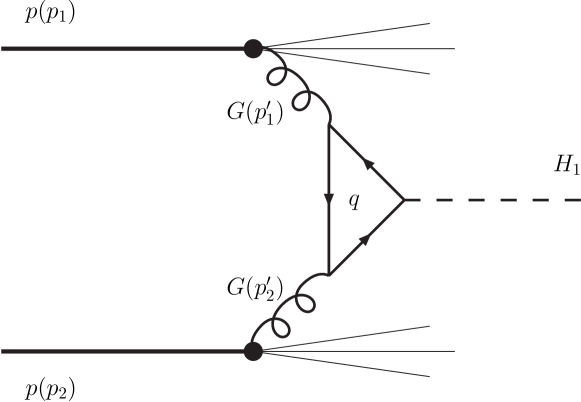
Figure 13: Diagram for the production of a Higgs particle $H_{1}$ by gluon–gluon fusion in proton–proton collisions.

$$\left.\sigma(p(p_{1})+p(p_{2})\rightarrow H_{1}+X)\right|_{GG-\text{fusion}}=\\ \frac{\pi^{2}\Gamma(H_{1}\rightarrow GG)}{8\;s\;m_{H_{1}}}F_{GG}\big{(}\frac{m_{H_{1}}^{2}}{s}\big{)}\;,$$ (57)

where $H_{1}=\rho^{\prime},h^{\prime}$, and $h^{\prime\prime}$. The function $F_{GG}$ is defined as

$$F_{GG}\bigg{(}\frac{m_{H_{1}}^{2}}{s}\bigg{)}\!=\!\!\int\limits_{0}^{1}dx_{1}N_{G}^{p}(x_{1})\int\limits_{0}^{1}dx_{2}N_{G}^{p}(x_{2})\delta\big{(}x_{1}x_{2}-\frac{m_{H_{1}}^{2}}{s}\big{)}$$ (58)

with $N_{G}^{p}(x)$ the gluon distribution function of the proton at LHC energies. Furthermore, $\Gamma(H_{1}\rightarrow GG)$ is the partial decay width for $H_{1}$ decaying into two gluons as discussed in Sect. 3.4.

Setting $H_{1}=\rho^{\prime}$ in (57) and using $\Gamma(\rho^{\prime}\rightarrow GG)$ from (LABEL:eq37) we get the cross section for $\rho^{\prime}$ production via gluon–gluon fusion in the MCPM. The result as shown in Fig. 14 is valid in the strict symmetry limit of the MCPM and coincides with that from the SM for $\rho^{\prime}_{SM}$; see for instance Djouadi:2005gi . Setting successively $H_{1}=h^{\prime}$ and $H_{1}=h^{\prime\prime}$ in (57) we obtain with (LABEL:eq38) and (LABEL:eq39) our estimates, in the sense discussed at the end of Sect. 3, for the corresponding production cross sections as shown in Fig. 14. Again, we give in Fig. 14 also the cross sections for Higgs-boson production via gluon–gluon fusion in proton–antiproton collisions at $\sqrt{s}=1.96$ TeV.

Figure 14: The cross sections for the production of $\rho^{\prime}$, $h^{\prime}$ and $h^{\prime\prime}$ via gluon–gluon fusion as functions of the Higgs-boson masses in proton–proton collisions at a c.m. energy of $\sqrt{s}=14~{}\text{TeV}$ (full lines) and in proton–antiproton collisions at $\sqrt{s}=1.96~{}\text{TeV}$ (dashed lines), respectively.

5 Discussion and conclusions

In this article we have given phenomenological predictions for proton–proton collisions at LHC energies in the framework of a two-Higgs-doublet model satisfying the principle of maximal CP invariance as introduced in Maniatis:2007de . In this maximally-CP-symmetric model (MCPM) there are three neutral Higgs particles, $\rho^{\prime}$, $h^{\prime}$ and $h^{\prime\prime}$, and one charged Higgs-boson pair $H^{\pm}$. We have investigated the decays of these particles. The Higgs particle $\rho^{\prime}$ behaves practically as the Higgs particle $\rho^{\prime}_{SM}$ in the SM. Only the $2\gamma$ widths of $\rho^{\prime}$ and $\rho^{\prime}_{SM}$ may differ substantially for $m_{\rho^{\prime}}\gtrsim 300$ GeV. The particles $h^{\prime}$, $h^{\prime\prime}$ and $H^{\pm}$, on the other hand, are predicted to have quite interesting properties. They couple to the fermions of the second family with coupling constants given by the masses of the third family. As a consequence the main decays of these Higgs particles are the fermionic ones of Tab. 3 if the Higgs masses are below about $400~{}\text{GeV}$. For larger Higgs-boson masses, the decay into a lighter Higgs boson associated with a gauge boson may become dominant, as shown in examples by the branching ratios in Figs. 8 and 9.

We have studied the production of the Higgs bosons $h^{\prime}$ and $h^{\prime\prime}$ in proton–proton and proton–antiproton collisions via quark–antiquark and gluon–gluon fusion. We have found that the much higher gluon densities compared to the quark densities in the proton do not compensate the loop suppression of the leading order gluon–gluon fusion process. Thus we find the Drell–Yan process with the annihilation of $c\bar{c}$ quarks dominating the production cross sections for $h^{\prime}$ and $h^{\prime\prime}$. The Drell–Yan process also leads to a similar production cross section for $H^{+}$ and $H^{-}$ via the annihilation of $c\bar{s}$ and $s\bar{c}$ quarks, respectively. In this way we get for the Higgs bosons $h^{\prime}$, $h^{\prime\prime}$ and $H^{\pm}$, if their masses are below $400$ GeV, quite high production cross sections exceeding $100$ pb at LHC energies. This is shown in Fig. 12. With an integrated luminosity of $100$ fb^-1 this translates into the production of more than $10^{8}$ Higgs bosons of the types $h^{\prime}$, $h^{\prime\prime}$ and $H^{\pm}$ if their masses are around 200 GeV. For Higgs-boson masses of $400$ GeV the number of produced particles $h^{\prime}$, $h^{\prime\prime}$ and $H^{\pm}$ is predicted to be of order $10^{7}$. These produced Higgs bosons will mainly decay into $c$- and $s$-quarks giving two jets. But, of course, there is a very large background from ordinary QCD two-jet events. Perhaps it will be possible to detect the Higgs-boson production events over the QCD background using $c$-quark tagging. Clearly, this presents an experimental challenge. A further possibility is to use the information from the angular distribution of the two jets. For the decays of the scalar particles $h^{\prime}$, $h^{\prime\prime}$ and $H^{\pm}$ the two-jet angular distributions must be isotropic in the rest frame of the decaying particle. Contrary to this, the QCD two-jet events are peaked in the beam directions. Clearly, only a detailed Monte Carlo study including an investigation of the QCD background and the detector resolution can tell if the particles $h^{\prime}$, $h^{\prime\prime}$ and $H^{\pm}$ are observable in their two-jet decays with the LHC detectors.

A promising signal for detecting the Higgs bosons $h^{\prime}$, $h^{\prime\prime}$ and $H^{\pm}$ of the MCPM is provided by their leptonic decays

$$\begin{split}h^{\prime}\rightarrow&\mu^{+}\mu^{-}\;,\\ h^{\prime\prime}\rightarrow&\mu^{+}\mu^{-}\;,\\ H^{+}\rightarrow&\mu^{+}\nu_{\mu}\;,\\ H^{-}\rightarrow&\mu^{-}\bar{\nu}_{\mu}\;.\end{split}$$ (59)

In (47) we have estimated the branching fractions for these decays to be about $3\times 10^{-5}$ for Higgs-boson masses below 400 GeV. With an integrated luminosity of 100 fb^-1 and the number of produced Higgs bosons given above we predict then around 3000 leptonic events for each of the channels in (59) if the Higgs-boson masses are around 200 GeV. For Higgs-boson masses of 400 GeV we still have 300 leptonic events for each of the decays in (59). We emphasize that a distinct feature of the MCPM is that decays involving the leptons $\tau$ and $\nu_{\tau}$ as well as $e$ and $\nu_{e}$ should be highly suppressed compared to the muonic channels (59). We may note that the $\mu^{+}\mu^{-}$ channel will be prominent at the LHC for the search for new effects including for instance heavy $Z^{\prime}$ bosons or Kaluza–Klein particles, see for instance cms:tdr ; atlas:tdr . Thus, the suppression of the $\tau$ and $e$ channels for the Higgs bosons of the MCPM may be an important way for distinguishing the MCPM from other possibilities for physics beyond the SM.

To conclude, we have in this article presented concrete predictions for the production and decay of the Higgs bosons of the MCPM. We found the Drell–Yan type process to be the dominant production mechanism. But, of course, there are also other mechanisms, which we hope to investigate in future work, for instance, Higgs-strahlung in quark–quark collisions. Thus, the predicted numbers of produced Higgs bosons given above for the LHC are in fact lower limits. We are looking forward to the start up of the experimentation at the LHC, where it should be possible to check our predictions.

Appendix A The Lagrangian after EWSB

The task is to express the Lagrangian $\mathscr{L}$ of the MCPM in terms of physical fields in the unitary gauge. This Lagrangian is given by

$$\mathscr{L}=\mathscr{L}_{\varphi}+\mathscr{L}_{\mathrm{Yuk}}+\mathscr{L}_{\mathrm{FB}}$$ (A.1)

where $\mathscr{L}_{\mathrm{FB}}$ is the standard gauge kinetic term for the fermions and gauge bosons; see for instance Nachtmann:1990ta . The Higgs-boson Lagrangian is denoted by $\mathscr{L}_{\varphi}$, the Yukawa term, giving the coupling of the fermions to the Higgs fields, by $\mathscr{L}_{\mathrm{Yuk}}$. In Maniatis:2007vn ; Maniatis:2007de the form for $\mathscr{L}_{\varphi}$ and $\mathscr{L}_{\mathrm{Yuk}}$ was derived from the requirement of maximal CP invariance, absence of flavor-changing neutral currents and absence of mass-degenerate massive fermions. For $\mathscr{L}_{\varphi}$ the result is

$$\mathscr{L}_{\varphi}=\sum\limits_{i=1,2}\big{(}D_{\mu}\varphi_{i}\big{)}^{\dagger}\big{(}D^{\mu}\varphi_{i}\big{)}-V(\varphi_{1},\varphi_{2})\;,$$ (A.2)

where $D_{\mu}$ are the covariant derivatives and $V$ is given in (11). The Yukawa term, $\mathscr{L}_{\mathrm{Yuk}}$, is given in (2).

Using the unitary gauge we insert for the Higgs-boson fields $\varphi_{1}$ and $\varphi_{2}$ the expressions (15) and (16), respectively. In the following we use as independent parameters of the Lagrangian the fine structure constant $\alpha$, respectively $e=\sqrt{4\pi\alpha}$, the Fermi constant $G_{F}$, the mass $m_{Z}$ of the Z-boson, the Higgs-boson masses $m_{\rho^{\prime}}^{2}$, $m_{h^{\prime}}^{2}$, $m_{h^{\prime\prime}}^{2}$, $m_{H^{\pm}}^{2}$, see (17)-(20), and the fermion masses $m_{\tau}$, $m_{t}$, $m_{b}$; see (22). With this, the following parameters are dependent ones: $s_{W}\equiv\sin\theta_{W}$, $c_{W}\equiv\cos\theta_{W}$, where $\theta_{W}$ is the weak mixing angle, the mass $m_{W}$ of the W boson, and the VEV $v_{0}$. The corresponding tree-level expressions for them in terms of the independent parameters are

$$\begin{split}s_{W}^{2}&=\frac{1}{2}\bigg{[}1-(1-\frac{e^{2}}{\sqrt{2}G_{F}m_{Z}^{2}})^{1/2}\bigg{]}\,,\\ m_{W}^{2}&=\frac{m_{Z}^{2}}{2}\bigg{[}1+(1-\frac{e^{2}}{\sqrt{2}G_{F}m_{Z}^{2}})^{1/2}\bigg{]}\,,\\ v_{0}&=2^{-1/4}G_{F}^{-1/2}\,.\end{split}$$ (A.3)

Keeping this in mind we find for $K_{0}$–$K_{3}$ of (4), inserting (15) and (16),

$$\begin{split}K_{0}=&\frac{1}{2}(v_{0}+\rho^{\prime})^{2}+\frac{1}{2}(h^{\prime 2}+h^{\prime\prime 2})+H^{+}H^{-}\;,\\ K_{1}=&(v_{0}+\rho^{\prime})h^{\prime}\;,\\ K_{2}=&(v_{0}+\rho^{\prime})h^{\prime\prime}\;,\\ K_{3}=&\frac{1}{2}(v_{0}+\rho^{\prime})^{2}-\frac{1}{2}(h^{\prime 2}+h^{\prime\prime 2})-H^{+}H^{-}\;.\end{split}$$ (A.4)

We get from (A.1) the following explicit form of $\mathscr{L}$. The expression for the fermion–boson term $\mathscr{L}_{\mathrm{FB}}$ is standard and can be found for instance in Nachtmann:1990ta . For $\mathscr{L}_{\varphi}+\mathscr{L}_{\mathrm{Yuk}}$ we get

$$\mathscr{L}_{\varphi}+\mathscr{L}_{\mathrm{Yuk}}=\hfill$$

$$\phantom{\;+\;}\frac{1}{8}m_{\rho^{\prime}}^{2}v_{0}^{2}\;+\frac{1}{2}(\partial_{\mu}\rho^{\prime})(\partial^{\mu}\rho^{\prime})\hfill$$

$$+m_{W}^{2}W_{\mu}^{-}W^{+\,\mu}(1+\frac{\rho^{\prime}}{v_{0}})^{2}\hfill$$

$$+\frac{1}{2}m_{Z}^{2}Z_{\mu}Z^{\mu}(1+\frac{\rho^{\prime}}{v_{0}})^{2}+(\partial_{\mu}H^{+})(\partial^{\mu}H^{-})\hfill$$

$$+\frac{1}{2}(\partial_{\mu}h^{\prime})(\partial^{\mu}h^{\prime})+\frac{1}{2}(\partial_{\mu}h^{\prime\prime})(\partial^{\mu}h^{\prime\prime})\\$$

$$-\frac{1}{2}m_{\rho^{\prime}}^{2}\big{(}\rho^{\prime 2}+\frac{1}{v_{0}}\rho^{\prime 3}+\frac{1}{4v_{0}^{2}}\rho^{\prime 4}\big{)}\\$$

$$-\frac{1}{2}m_{h^{\prime}}^{2}h^{\prime 2}-\frac{1}{2}(m_{\rho^{\prime}}^{2}+2m_{h^{\prime}}^{2})h^{\prime 2}\left[\frac{1}{v_{0}}\rho^{\prime}+\frac{1}{2v_{0}^{2}}\rho^{\prime 2}\right]\\$$

$$-\frac{1}{2}m_{h^{\prime\prime}}^{2}h^{\prime\prime 2}-\frac{1}{2}(m_{\rho^{\prime}}^{2}+2m_{h^{\prime\prime}}^{2})h^{\prime\prime 2}\left[\frac{1}{v_{0}}\rho^{\prime}+\frac{1}{2v_{0}^{2}}\rho^{\prime 2}\right]\\$$

$$-m_{H^{\pm}}^{2}H^{+}H^{-}-(m_{\rho^{\prime}}^{2}+2m_{H^{\pm}}^{2})H^{+}H^{-}\left[\frac{1}{v_{0}}\rho^{\prime}+\frac{1}{2v_{0}^{2}}\rho^{\prime 2}\right]\\$$

$$-\frac{m_{\rho^{\prime}}^{2}}{2v_{0}^{2}}\bigg{[}\frac{1}{4}(h^{\prime 4}+h^{\prime\prime 4}+2h^{\prime 2}h^{\prime\prime 2})\\ +(h^{\prime 2}+h^{\prime\prime 2})H^{+}H^{-}+(H^{+})^{2}(H^{-})^{2}\bigg{]}\\$$

$$+ie\big{(}\frac{c_{W}^{2}-s_{W}^{2}}{2s_{W}c_{W}}Z^{\mu}+A^{\mu}\big{)}\big{(}H^{+}\partial_{\mu}H^{-}-H^{-}\partial_{\mu}H^{+}\big{)}\\$$

$$+\frac{e}{2s_{W}c_{W}}Z^{\mu}\big{(}h^{\prime\prime}\partial_{\mu}h^{\prime}-h^{\prime}\partial_{\mu}h^{\prime\prime}\big{)}\\$$

$$+\frac{ie}{2s_{W}}W^{+\,\mu}\big{(}h^{\prime}\partial_{\mu}H^{-}-H^{-}\partial_{\mu}h^{\prime}\big{)}\\$$

$$-\frac{ie}{2s_{W}}W^{-\,\mu}\big{(}h^{\prime}\partial_{\mu}H^{+}-H^{+}\partial_{\mu}h^{\prime}\big{)}\\$$

$$-\frac{e}{2s_{W}}W^{+\,\mu}\big{(}h^{\prime\prime}\partial_{\mu}H^{-}-H^{-}\partial_{\mu}h^{\prime\prime}\big{)}\\$$

$$-\frac{e}{2s_{W}}W^{-\,\mu}\big{(}h^{\prime\prime}\partial_{\mu}H^{+}-H^{+}\partial_{\mu}h^{\prime\prime}\big{)}\\$$

$$+e^{2}\bigg{[}\left(\frac{c_{W}^{2}-s_{W}^{2}}{2s_{W}c_{W}}\right)^{2}Z_{\mu}Z^{\mu}H^{+}H^{-}\\ +\frac{c_{W}^{2}-s_{W}^{2}}{s_{W}c_{W}}Z_{\mu}A^{\mu}H^{+}H^{-}+A_{\mu}A^{\mu}H^{+}H^{-}\bigg{]}\\$$

$$+\frac{e^{2}}{8s_{W}^{2}c_{W}^{2}}Z_{\mu}Z^{\mu}(h^{\prime 2}+h^{\prime\prime 2})\\$$

$$+\frac{e^{2}}{2s_{W}^{2}}W_{\mu}^{+}W^{-\,\mu}\big{(}\frac{1}{2}h^{\prime 2}+\frac{1}{2}h^{\prime\prime 2}+H^{+}H^{-}\big{)}\\$$

$$+\frac{e^{2}}{2s_{W}}\big{(}-\frac{s_{W}}{c_{W}}Z_{\mu}+A_{\mu}\big{)}W^{+\,\mu}H^{-}h^{\prime}\\$$

$$+\frac{e^{2}}{2s_{W}}\big{(}-\frac{s_{W}}{c_{W}}Z_{\mu}+A_{\mu}\big{)}W^{-\,\mu}H^{+}h^{\prime}\\$$

$$+\frac{ie^{2}}{2s_{W}}\big{(}-\frac{s_{W}}{c_{W}}Z_{\mu}+A_{\mu}\big{)}W^{+\,\mu}H^{-}h^{\prime\prime}\\$$

$$-\frac{ie^{2}}{2s_{W}}\big{(}-\frac{s_{W}}{c_{W}}Z_{\mu}+A_{\mu}\big{)}W^{-\,\mu}H^{+}h^{\prime\prime}\\$$

$$-m_{\tau}\bar{\tau}\tau\big{(}1+\frac{1}{v_{0}}\rho^{\prime}\big{)}\\$$

$$-m_{t}\bar{t}t\big{(}1+\frac{1}{v_{0}}\rho^{\prime}\big{)}\\$$

$$-m_{b}\bar{b}b\big{(}1+\frac{1}{v_{0}}\rho^{\prime}\big{)}\\$$

$$+\frac{m_{\tau}}{v_{0}}\bar{\mu}\mu h^{\prime}+\frac{m_{t}}{v_{0}}\bar{c}ch^{\prime}+\frac{m_{b}}{v_{0}}\bar{s}sh^{\prime}\\$$

$$+\frac{im_{\tau}}{v_{0}}\bar{\mu}\gamma_{5}\mu h^{\prime\prime}-\frac{im_{t}}{v_{0}}\bar{c}\gamma_{5}ch^{\prime\prime}+\frac{im_{b}}{v_{0}}\bar{s}\gamma_{5}sh^{\prime\prime}\\$$

$$+\frac{m_{\tau}}{\sqrt{2}v_{0}}\left[\bar{\nu}_{\mu}(1+\gamma_{5})\mu H^{+}+\bar{\mu}(1-\gamma_{5})\nu_{\mu}H^{-}\right]\\$$

$$-\frac{1}{\sqrt{2}v_{0}}\bigg{\{}\bar{c}\;\big{[}m_{t}(1-\gamma_{5})-m_{b}(1+\gamma_{5})\big{]}\;sH^{+}\\ +\bar{s}\;\big{[}m_{t}(1+\gamma_{5})-m_{b}(1-\gamma_{5})\big{]}\;cH^{-}\bigg{\}}.\\$$ (A.5)

From (A.5) it is easy to read off the Feynman rules in the unitary gauge. We list here only the Higgs-boson–fermion vertices and the vertices for two Higgs bosons and one gauge boson. The arrow on the $W$ and $H$ lines indicates the flow of negative charge. In case a momentum occurs in the Feynman rules, the momentum direction is indicated by an extra arrow.
$-i\frac{m_{\tau}}{v_{0}}$
$-i\frac{m_{t}}{v_{0}}$
$-i\frac{m_{b}}{v_{0}}$
$i\frac{m_{\tau}}{v_{0}}$
$i\frac{m_{t}}{v_{0}}$
$i\frac{m_{b}}{v_{0}}$
$-\frac{m_{\tau}}{v_{0}}\gamma_{5}$
$\frac{m_{t}}{v_{0}}\gamma_{5}$
$-\frac{m_{b}}{v_{0}}\gamma_{5}$
$i\frac{m_{\tau}}{\sqrt{2}v_{0}}(1+\gamma_{5})$
$i\frac{m_{\tau}}{\sqrt{2}v_{0}}(1-\gamma_{5})$
$-i\frac{1}{\sqrt{2}v_{0}}\big{[}m_{t}(1-\gamma_{5})-m_{b}(1+\gamma_{5})\big{]}$
$-i\frac{1}{\sqrt{2}v_{0}}\big{[}m_{t}(1+\gamma_{5})-m_{b}(1-\gamma_{5})\big{]}$
$ie(p+p^{\prime})_{\mu}$
$ie\frac{c_{W}^{2}-s_{W}^{2}}{2s_{W}c_{W}}(p+p^{\prime})_{\mu}$
$\frac{e}{2s_{W}c_{W}}(p+p^{\prime})_{\mu}$
$i\frac{e}{2s_{W}}(p+p^{\prime})_{\mu}$
$i\frac{e}{2s_{W}}(p+p^{\prime})_{\mu}$
$-\frac{e}{2s_{W}}(p+p^{\prime})_{\mu}$
$\frac{e}{2s_{W}}(p+p^{\prime})_{\mu}$

References

- (1) C. Amsler et al. [Particle Data Group], Phys. Lett. B 667 (2008) 1.
- (2) J. Ellis, AIP Conf. Proc. 957, 38 (2007) [arXiv:0710.0777 [hep-ph]].
- (3) M. Kobayashi and T. Maskawa, Prog. Theor. Phys. 49 (1973) 652
- (4) J. F. Gunion, H. E. Haber, G. L. Kane and S. Dawson, “The Higgs Hunter’s Guide”, Addison–Wesley, (1990).
- (5) G. Cvetic, Phys. Rev. D 48, 5280 (1993) [hep-ph/9309202].
- (6) I. F. Ginzburg and M. Krawczyk, Phys. Rev. D 72 115013 (2005) [hep-ph/0408011].
- (7) J. F. Gunion and H. E. Haber, Phys. Rev. D 72 095002 (2005) [hep-ph/0506227v2].
- (8) R. Barbieri and L. J. Hall, “Improved naturalness and the two Higgs doublet model”, [hep-ph/0510243].
- (9) G. C. Branco, M. N. Rebelo and J. I. Silva-Marcos, Phys. Lett. B 614 (2005) 187 [hep-ph/0502118].
- (10) C. C. Nishi, Phys. Rev. D 74 036003 (2006) [hep-ph/0605153].
- (11) R. Barbieri, L. J. Hall and V. S. Rychkov, Phys. Rev. D 74 015007 (2006) [hep-ph/0603188].
- (12) I. P. Ivanov, Phys. Rev. D 75 035001 (2007) [hep-ph/0609018].
- (13) L. Fromme, S. J. Huber and M. Seniuch, JHEP 0611 (2006) 038 [hep-ph/0605242].
- (14) I. P. Ivanov, Phys. Rev. D 77, 015017 (2008) [arXiv:0710.3490 [hep-ph]].
- (15) A. Barroso, P. M. Ferreira and R. Santos, Phys. Lett. B 652 (2007) 181 [hep-ph/0702098].
- (16) J. M. Gerard and M. Herquet, Phys. Rev. Lett. 98 (2007) 251802 [hep-ph/0703051].
- (17) M. Maniatis, A. von Manteuffel, O. Nachtmann and F. Nagel, Eur. Phys. J. C 48, 805 (2006) [hep-ph/0605184].
- (18) M. Maniatis, A. von Manteuffel and O. Nachtmann, Eur. Phys. J. C 57, 719 (2008) [arXiv:0707.3344 [hep-ph]].
- (19) M. Maniatis, A. von Manteuffel and O. Nachtmann, Eur. Phys. J. C 57, 739 (2008) [arXiv:0711.3760 [hep-ph]].
- (20) C. Buttar et al., “Les Houches physics at TeV colliders 2005, standard model, QCD, EW, and Higgs working group: Summary report”, [hep-ph/0604120].
- (21) C. S. Kim, C. Yu and K. Y. Lee, “Probing CP violating two Higgs doublet model through interplay between LHC and ILC”, [hep-ph/0602076].
- (22) A. Djouadi, Phys. Rept. 457 (2008) 1 [hep-ph/0503172].
- (23) The CMS Collaboration 2007, J. Phys. G: Nucl. Part. Phys. 34 995 (2007), [hep-ph/0602076].
- (24) The ATLAS Collaboration, ATLAS TDR 14, CERN/LHCC 99-14, Vol. 2, (1999), available at http://atlas.web.cern.ch/Atlas/GROUPS/PHYSICS/TDR/access.html.
- (25) O. Nachtmann, “Elementary Particle Physics: Concepts And Phenomena”, Springer, Berlin (1990).