The Large–Scale Environments of Type Ia Supernovae: Evidence for a Metallicity Bias in the Rate or Luminosity of Prompt Ia Events

Abstract

Using data drawn from the Sloan Digital Sky Survey (SDSS) and the SDSS–II Supernova Survey, we study the local environments of confirmed type Ia supernovae (SNe Ia) in the nearby Universe. At $0.05<z<0.15$, we find that SN Ia events in blue, star–forming galaxies occur preferentially in regions of lower galaxy density relative to galaxies of like stellar mass and star–formation rate, while SNe Ia in nearby red galaxies show no significant environment dependence within the measurement uncertainties. Even though our samples of SNe in red hosts are relatively small in number, tests on simulated galaxy samples suggest that the observed distribution of environments for red SN Ia hosts is in poor agreement with a cluster type Ia rate strongly elevated relative to the field rate. Finally, after considering the impact of galaxy morphology, stellar age, stellar metallicity, and other relevant galaxy properties, we conclude that the observed correlation between the SN Ia rate and environment in the star–forming galaxy population is likely driven by a gas–phase metallicity effect, such that prompt type Ia supernovae occur more often or are more luminous in metal–poor systems.

1. Introduction

Type Ia supernovae (SNe Ia) are thought to be distinct from other types of supernovae (that is, resulting from a different progenitor population), as they are found in galaxies spanning a broad range of properties. While, type II, Ib, and Ic SNe are only found in star–forming galaxies, indicating that they are the evolutionary product of massive stars, SNe Ia are found in both star–forming and quiescent systems, suggesting that they are somehow connected to the evolution of less–massive stars (e.g., Oemler & Tinsley, 1979; van den Bergh, 1990; della Valle & Livio, 1994; Cappellaro et al., 1999). In particular, it is widely accepted that the progenitors of type Ia supernovae are carbon–oxygen white dwarfs (WDs), which have accreted mass up to the Chandrasekhar limit (Chandrasekhar, 1931), perhaps via deposition from a binary companion (Whelan & Iben, 1973; Han & Podsiadlowski, 2004). Lending support to this picture, theoretical models of exploding WDs (e.g., Kasen & Plewa, 2005; Kasen & Woosley, 2007) are able to reproduce the properties of SN Ia spectra, including the lack of hydrogen features and the presence of strong silicon absorption, which define the type Ia classification.

Recent observations of the type Ia SN rate in local and intermediate–redshift galaxies have cast some doubt on — or at minimum confused — the theoretical paradigm just discussed. If SNe Ia are simply the product of old stellar populations (i.e., an evolutionary outcome of low–mass stars), then the SN Ia rate should depend strongly on stellar mass, while being independent of the level of on–going star–formation activity (at fixed stellar mass). While the type Ia rate is found to depend on stellar mass, it is also found to be greater per unit stellar mass in galaxies with higher specific star–formation rates (Mannucci et al., 2005; Sullivan et al., 2006b). These current observations of the supernova Ia rate support a revised theoretical model (e.g., Scannapieco & Bildsten, 2005; Mannucci et al., 2006; Pritchet et al., 2008), perhaps one employing a two–component progenitor distribution with a “prompt” component correlated with star–formation activity and a “delayed” component correlated with stellar mass (i.e., the underlying older stellar population). Still, despite uncertainty in the nature of the two observed components of the type Ia rate as well as difficulties in directly observing the progenitors of type Ia events, current observations remain consistent with a progenitor population comprised entirely of carbon–oxygen WDs, allowing for an increasingly broad distribution of delay times (e.g., Greggio et al., 2008).

Studying the environments of supernova — i.e., their place in the hierarchy of large–scale structure — may prove useful in shedding light on the nature of the two components of the type Ia rate or on the nature of the underlying progenitor population or potentially even revealing dependencies of the type Ia rate or luminosity on galaxy properties that are correlated with environment. Type Ia supernovae are often used as cosmological probes, allowing distances to be measured out to intermediate redshifts and providing constraints on cosmological parameters such as $H_{0}$, $\Omega_{M}$, and $\Omega_{\Lambda}$ (Riess et al., 1998; Perlmutter et al., 1999). Understanding any relationship between host galaxy properties and type Ia luminosity is critical for minimizing systematic effects that might bias studies of distant type Ia supernovae and limit our abilities to constrain cosmological models. Along these lines, environment can be utilized as a proxy for other galaxy properties that are otherwise difficult to constrain observationally (e.g., stellar metallicity or age). For instance, a galaxy of the same stellar mass as another, but located in a higher–density environment, will generally have formed earlier in the history of the Universe and will contain older stellar populations as a result (e.g., Schaye et al., 2003; Davé et al., 2006).

Understanding if the type Ia rate varies with the local galaxy environment may provide new insights into the true nature of the progenitor population, while also shedding light on many aspects of galaxy formation and evolution. For instance, using environment as a proxy for formation time could be helpful in interpreting the role of an evolving initial stellar mass function (e.g., Davé, 2008; van Dokkum, 2008) in establishing the potential progenitor population.

More directly, constraining the correlation between the SN rate (of both type Ia and II events) and galaxy environment is also critical for understanding various details of the chemical enrichment and star–formation histories of galaxies. For example, supernovae govern the production of metals (Woosley & Weaver, 1995; Sato et al., 2007), with types Ia and II dominating iron and oxygen production, respectively. Due to their large gravitational potential wells, galaxy clusters are potentially the only systems to have retained all of the metals produced by stars. For this reason, studies of the metal content (e.g., Fe abundance) in the intracluster medium (ICM) provide interesting windows on the cosmic star–formation history (e.g., Matteucci & Vettolani, 1988; Calura et al., 2007). Given the role of supernovae in dispersing metals, a critical part of this picture is to understand how the SN rate may vary with environment in addition to time (Sivanandam et al., 2008).

Furthermore, energy injected into the interstellar medium (ISM) by supernovae could play an important role in influencing the formation of galactic disks (Scannapieco et al., 2008). Variation in the supernova rate with environment could thus be a factor (though likely very weak) in the establishment of the morphology–density relation (e.g., Davis & Geller, 1976; Dressler, 1980). Finally, feedback from supernova–generated winds is thought to be an essential part of shaping the mass–metallicity relation (Dekel & Silk, 1986; Cole, 1991), causing a downturn in the relative enrichment at low stellar masses by ejecting metals into the intergalactic medium (IGM). Understanding the correlation between supernova rates and environment will help reveal whether supernova feedback is also responsible for driving the scatter in this fundamental relation, causing the observed correlation between metallicity and environment at fixed stellar mass and star–formation rate (Cooper et al., 2008a).

In this paper, we utilize public data from the Sloan Digital Sky Survey (SDSS, York et al., 2000) and from the SDSS–II Supernova Survey (Frieman et al., 2008) to examine the environments of local type Ia SNe. In §2, we discuss the data samples employed along with our measurements of galaxy environments. Our main results regarding the environments of type Ia SNe are presented in §3, with comparison to related work, analysis of potential selection effects, and further discussion in §4. Finally, in §5, we summarize our conclusions. Throughout this paper, we assume a flat $\Lambda$CDM cosmology with $\Omega_{m}=0.3$, $\Omega_{\Lambda}=0.7$, $w=-1$, and a Hubble parameter of $H_{0}=100\ {\rm km}\ {\rm s}^{-1}\ {\rm Mpc}^{-1}$, unless otherwise noted.

2. The Data Sets

2.1. The Supernova Sample

Over the past three years, the SDSS–II Supernova Survey (Frieman et al., 2008; Sako et al., 2008) has repeatedly scanned a $300$ square degree region around the celestial equator in the southern Galactic hemisphere in search of supernovae. The resulting data set, which includes more than $800$ SNe, is exceptional in its size and uniformity, significantly increasing the number of known supernovae at $z\lesssim 0.3$ with well–sampled and well–calibrated light curves. Only the Supernova Legacy Survey (SNLS, Astier et al., 2006), which primarily targets supernovae at higher redshifts $(z>0.3)$, has discovered a comparable number of type Ia events.

In this work, we utilize the $>\!500$ confirmed SNe Ia from the SDSS–II Supernova Survey. We limit the sample to a redshift range of $0.05<z<0.15$ and to SNe for which a spectrum was obtained, which yields a total sample size of 163 type Ia SNe (SN–A sample). We exclude type II supernovae from our analysis due to their limited numbers; there is only one type II supernova for every $\sim\!10$ type Ia event in the SDSS–II Supernovae Survey catalog. While type II events are more numerous than SNe Ia (e.g., Maoz, 2008), they are intrinsically fainter and thus less–likely to be detected in a magnitude–limited survey.

A key aspect of the SDSS–II Supernova Survey is the general spatial uniformity of the number of imaging epochs. That is, there is little spatial dependence to the on–sky cadence of the survey (see Figure 1 of Frieman et al., 2008, and Sako et al. 2008). This translates to a survey that is equally sensitive to supernovae in all environments, which therefore allows for direct comparison of the environments of SN hosts to the environments of the global galaxy population.

2.2. The Galaxy Sample

With spectra and multi–band photometry for more than $500,000$ galaxies, the SDSS Data Release 6 (DR6, Adelman-McCarthy et al., 2008) enables the local density of galaxies (which we refer to throughout this paper as “environment”) at $z\lesssim 0.2$ to be measured over approximately one quarter of the sky, including nearly the entire area surveyed by the SDSS–II Supernova Survey. We select a sample of $553,188$ galaxies from the SDSS DR6, as contained in the New York University Value–Added Galaxy Catalog (NYU–VAGC, Blanton et al., 2005b). This sample is limited to the redshift range $0.01<z<0.3$ and to SDSS fiber plates for which the redshift success rate for targets in the main spectroscopic survey is 80 per cent or greater.

For each galaxy, the SDSS/NYU–VAGC database provides precise information about position on the plane of the sky ($<\!0.1$ arcsecond rms per coordinate) and along the line of sight ($\Delta z\sim 0.0001$, Abazajian et al., 2004), enabling the local environment to be accurately characterized (see §2.4). In addition, rest–frame colors and absolute magnitudes are computed using the KCORRECT $K$–correction code (version v4_1_4) of Blanton & Roweis (2007, see also ). The rest–frame quantities for the SDSS sample are derived from the apparent $ugriz$ model magnitudes in the SDSS DR6, where all SDSS magnitudes within this paper are calibrated to the AB system (Oke & Gunn, 1983).

As shown by many previous studies at low and intermediate redshift (e.g., Strateva et al., 2001; Bell et al., 2004; Willmer et al., 2006) and as illustrated in Figure 1, the distribution of galaxies in color–magnitude space is bimodal, with a tight red sequence and a more diffuse blue cloud. To divide the SDSS galaxy sample into these two broad classes, we use the following magnitude–dependent cut:

$$g-r=-0.02667\cdot M_{r}+0.11333.$$ (1)

This division in rest–frame $g-r$ color is shown in Fig. 1 as the dashed red line.

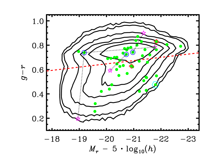
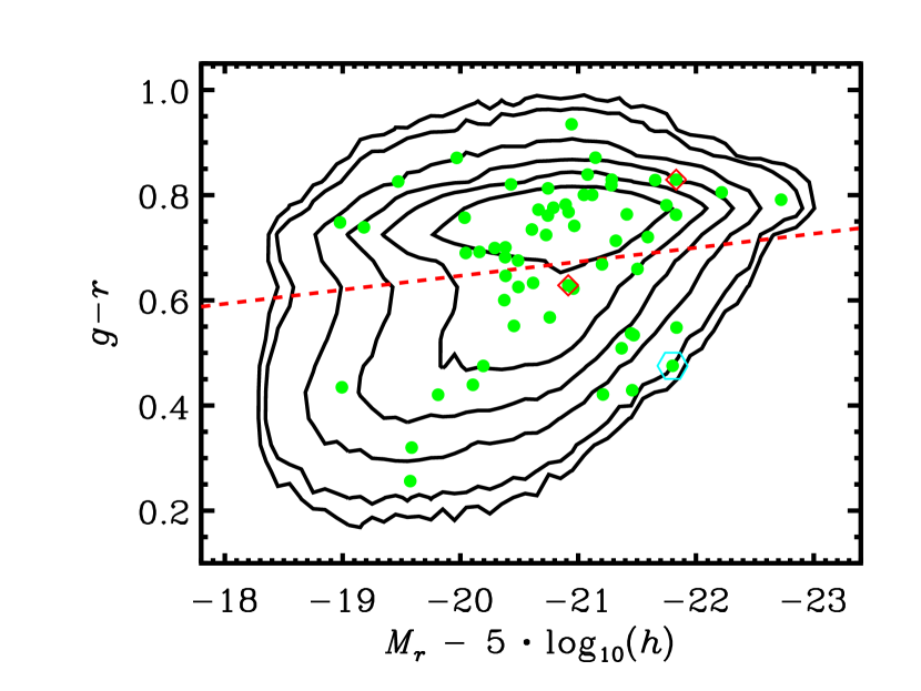
Figure 1.— (Left) We plot the rest–frame $g-r$ versus $M_{r}$ color–magnitude distribution for SDSS galaxies in the spectroscopic sample within the redshift range $0.05<z<0.15$. Due to the large number of galaxies in the sample, we plot contours (rather than individual points) corresponding to 25, 50, 200, 500, 1000, and 2000 galaxies per bin of $\Delta(g-r)=0.05$ and $\Delta M_{r}=0.1$. The dashed red horizontal line shows the division between the red sequence and the blue cloud as given in Equation 1. The green points correspond to the $48$ SN Ia host galaxies included in sample SN–B, where the two galaxies within $1\>h^{-1}$ comoving Mpc of a survey edge are outlined by red diamonds. The cyan hexagon identifies one particular host, which is a low–redshift QSO. The blue circles outlining three of the green points denote the three SNe with ambiguous host identifications. The magenta stars (connected by dotted lines to the corresponding blue circle) illustrate the location in color–magnitude space of the other potential hosts. In one case, there are three possible hosts in the spectroscopic sample. Finally, note that the SN hosts are divided roughly evenly between the red sequence and the blue cloud. (Right) Same as plotted on the left, except that the green points show the rest–frame $g-r$ versus $M_{r}$ color–magnitude distribution for the $60$ SN Ia host galaxies in sample SN–C. Again, the two galaxies within $1\>h^{-1}$ comoving Mpc of a survey edge are outlined by red diamonds and the one SN hosted by a QSO is marked by the cyan hexagon.

Stellar masses are computed for each galaxy in the SDSS sample, again using the KCORRECT package with template spectral energy distributions (SEDs) based on those of Bruzual & Charlot (2003). To estimate stellar masses, the best–fitting SED given the observed $ugriz$ photometry and spectroscopic redshift is used to directly compute the stellar mass–to–light ratio $({\rm M}_{*}/L)$, assuming a Chabrier (2003) initial mass function.

Due to the large wavelength coverage of the SDSS spectra ($3800$–$9200$Å), star–formation rates (SFRs) are able to be estimated for nearly every galaxy in the spectroscopic catalog based on the measured H$\alpha$ $(\lambda 6563{\rm\AA})$ line emission. For each galaxy in the spectroscopic sample, emission–line fluxes and equivalent widths (EWs) are measured by fitting for and subtracting the stellar continuum, as detailed by Yan et al. (2006). To derive the line luminosity and correct for aperture effects related to the finite size of the SDSS fibers, we estimate the total H$\alpha$ luminosity by combining measurements of the H$\alpha$ EW with the $K$–corrected broad–band absolute magnitudes (i.e., assuming that the ratio of the line emission to the broad–band flux is uniform across the entire galaxy).

Star–formation rates are inferred from the measured H$\alpha$ luminosities according to the relation given by Kennicutt (1998):

$$\psi({\rm H}\alpha)=7.9\times 10^{-42}\frac{L({\rm H}\alpha)}{{\rm ergs}\ {{\rm s}^{-1}}}{\rm M}_{\sun}\ {\rm yr}^{-1},$$ (2)

where $L({\rm H}\alpha)$ is corrected by a factor of 2.8 to account for underlying dust attenuation and stellar absorption. In a small percentage of cases $(<\!15\%)$, the H$\alpha$ flux is unable to be measured accurately due to bad pixels within the emission–line or continuum windows. In these instances, we infer the SFR from the measured [O II] $\lambda 3727$Å line luminosity, corrected using the empirical calibration of Moustakas et al. (2006). Note that in computing our star–formation rates, we adopt a Hubble parameter, $h=0.7$, to match that calibration.

Our measured SFRs agree well with those measured for SDSS galaxies by Brinchmann et al. (2004), who used fits of emission–line and continuum properties to stellar population models (see also Charlot et al., 2002); through direct comparison with our inferred star–formation rates, we find an offset of $\sim\!0.3$ dex and a scatter of $\sim\!0.15$ dex relative to the Brinchmann et al. (2004) measurements, with the offset of the Brinchmann et al. (2004) SFRs to higher values largely due to differences in dust corrections. Direct comparison of our estimated H$\alpha$ luminosities to those of Moustakas et al. (2006) show excellent agreement, with only a small offset corresponding to a $\sim\!0.01$ dex offset and $\sim\!0.02$ dex scatter in the inferred star–formation rates.

In addition to the SDSS spectroscopic data set, we utilize the larger SDSS DR6 photometric catalog, which contains uniform, precision photometry for millions of sources down to a $5$–$\sigma$ limiting magnitude of $r=22.2$ in asinh magnitudes (Lupton et al., 1999). For all sources in the imaging catalog, we estimate rest–frame colors, absolute magnitudes, stellar masses, and photometric redshifts using the KCORRECT package. Due to the lack of spectral information, we are unable to estimate star–formation rates for sources in the imaging catalog.

2.3. Identifying Host Galaxies

For each supernova in the SDSS–II Supernova Survey sample, we attempt to identify a host galaxy within the SDSS DR6 spectroscopic and imaging data sets. When identifying hosts in the SDSS spectroscopic galaxy catalog, a projected, radial window of $25\>h^{-1}$ kpc (physical) is employed to distinguish potential hosts on the plane of the sky in conjunction with a velocity window of $\Delta v=3000\ {\rm km}\ {\rm s}^{-1}$ along the line of sight. This moderately–large velocity window is adopted to account for the relatively–low precision of the redshifts derived from SN Ia features ($\Delta z<0.005$, Frieman et al., 2008). If multiple SDSS galaxies fall within the radial window, then the galaxy closest in projected distance is taken as the host. A host is considered to be unambiguously identified, if one (and only one) galaxy is found within the search window.

In the redshift range $0.05<z<0.15$, a total of 48 type Ia supernovae (SN–B sample) are matched to host galaxies (45 of the 48 are matched unambiguously) in the SDSS spectroscopic catalog. The location of the host galaxies in color–magnitude space is given by the green points in Figure 1a; the hosts are roughly equally divided between the red sequence $(26/48)$ and the blue cloud $(22/48)$. We exclude one supernova from the SN–B sample due to its occurrence in a bright, nearby QSO (see the hexagon point in Fig. 1), for which measurements of luminosity and star–formation rate are highly uncertain.

Although the SDSS spectroscopic data set supplies relatively precise information about the line–of–sight position of many galaxies in the area surveyed by the SDSS–II Supernova Survey, the SDSS imaging catalog provides a significantly more complete census of the galaxy population due to its much greater depth; the SDSS imaging catalog is complete down to $r=22.2$, while the SDSS spectroscopic sample is magnitude–limited at $r\leq 17.77$. For this reason, we also search for host galaxies within the SDSS DR6 imaging catalog.

Using a magnitude–limited $(r\leq 19.5)$ imaging catalog, we identify potential hosts on the plane of the sky within a projected, circular window of $25\>h^{-1}$ kpc (physical) in radius. To differentiate between potential hosts along the line–of–sight, we compute the redshift for each galaxy in the imaging catalog, within the radial window, using the photometric–redshift code SDSS_KPHOTOZ in KCORRECT (version v4_1_4 Blanton et al., 2003a). Within a velocity window of $\Delta v=6000\ {\rm km}\ {\rm s}^{-1}$, we select the closest galaxy in projected distance as the host. A total of 60 type Ia supernovae in the redshift range $0.05<z<0.15$ (SN–C sample) are matched to host galaxies in the SDSS imaging catalog. The distribution of these hosts in color–magnitude space is given by the green points in Figure 1b; they are weighted more towards the red–sequence population relative to the hosts of the SN–B sample (36 out of 57 are red). The SN–C sample is a superset of the SN–B sample, with all of the supernovae in SN–B being matched to the same host galaxy. Again, we exclude the one supernova from the sample that is found within a local QSO.

2.4. Measuring the Local Environment

We consider the “environment” of a galaxy to be defined by the local mass overdensity, as traced by the local overdensity of galaxies; over quasi–linear regimes, the mass density and galaxy density should simply differ by a factor of the galaxy bias (Kaiser, 1987). To estimate the overdensity of galaxies in the SDSS, we utilize measurements of the projected fifth–nearest–neighbor surface density $(\Sigma_{5})$ about each galaxy, where the surface density depends on the projected distance to the fifth–nearest neighbor, $D_{p,5}$, as $\Sigma_{5}=5/(\pi D^{2}_{p,5})$. In computing $\Sigma_{5}$, a velocity window of $\pm 1500\ {\rm km}\ {\rm s}^{-1}$ is employed to exclude foreground and background galaxies along the line of sight. The projected distance to the N^th–nearest neighbor provides an accurate estimate of local galaxy density over a broad and continuous range of scales. As shown by Cooper et al. (2005), it is reasonably robust to redshift–space distortions, while also effectively tracing the local density in underdense regions.

To correct for the redshift dependence of the sampling rate of the SDSS, each surface density value is divided by the median $\Sigma_{5}$ of galaxies at that redshift within a window of $\Delta z=0.02$; this converts the $\Sigma_{5}$ values into measures of overdensity relative to the median density (given by the notation $1+\delta_{5}$ herein) and effectively accounts for redshift variations in the selection rate (Cooper et al., 2005). We restrict our analyses to the redshift range $0.04<z<0.16$, avoiding the low– and high–redshift tails of the SDSS $d{\rm N}/dz$ distribution where the variations in the survey selection rate are greatest. Finally, to minimize the effects of edges and holes in the SDSS survey geometry, we exclude all galaxies within $1\>h^{-1}$ Mpc (comoving) of a survey boundary, reducing our sample size to $392,938$ galaxies within the redshift range $0.04<z<0.16$.

For each supernova (those with and without an identified host in the SDSS DR6 galaxy catalog), we measure the local environment in a manner identical to that followed for the galaxy sample. That is, we measure the local surface density of galaxies about the position of the supernova, using the positional information $(\alpha,\delta,z)$ from the SDSS–II Supernova Survey and using the SDSS DR6 galaxy sample to trace the local environment. After excluding SNe near the survey boundary (within $1\>h^{-1}$ Mpc), we arrive at a final sample (SN–A) of $134$ SNe Ia. Note that for the subset of SNe with an identified host in the SDSS DR6 spectroscopic catalog (SN–B), higher–precision information about the local environment is also available by proxy via the host galaxy. A summary of all of the supernova samples is provided in Table 1.

2.5. Selecting Comparison Samples

As discussed in §1, a variety of recent observations have shown that the SN Ia rate (weighted by mass or by luminosity) depends on the properties of the host galaxy. For instance, Mannucci et al. (2005), using the supernova catalog of Cappellaro et al. (1999), showed that SNe Ia are more common in morphologically late–type galaxies (Irr and Sbc/d) relative to more bulge–dominated systems (E/S0). Similarly, recent work from the Supernova Legacy Survey (Sullivan et al., 2006a) found that the SN Ia rate is greater among galaxies with greater stellar mass and among galaxies with higher star–formation rates (Sullivan et al., 2006b).

For several decades, the observed properties of galaxies (including star–formation rates, morphology, and rest–frame color) have been known to depend upon the local environment (e.g., Davis & Geller, 1976; Postman & Geller, 1984; Balogh et al., 1998; Cooper et al., 2006). In particular, galaxies with more massive stellar populations tend to favor regions of higher galaxy density (Hogg et al., 2004; Zehavi et al., 2005), while systems with high star–formation rates typically reside in low–density environs in the local Universe (Gómez et al., 2003; Cooper et al., 2008b). In addition, the relationships between galaxy properties and environment depend on redshift, with the color–density and morphology–density relations growing weaker at higher $z$ (e.g., Dressler et al., 1997; Smith et al., 2005; Cooper et al., 2007) and the SFR–density relation inverting between $z\sim 1$ and $z\sim 0$ (Elbaz et al., 2007; Cooper et al., 2008b).

Given these known correlations between galaxy properties and [1] the SN Ia rate as well as [2] the local galaxy density, we extract multiple subsamples from the SDSS galaxy sample, selected to match the characteristics of the SN Ia samples, thereby enabling analysis of the local environments of SN hosts independent of selection biases connected to galaxy type. Since many of the SNe in the SN–A sample lack an identified host galaxy in the SDSS galaxy catalog, we are unable to select a comparison sample that matches properties such as luminosity, stellar mass, star–formation rate, etc. Here, we randomly select $15,000$ galaxies from the set of $392,938$ SDSS galaxies with accurate environment measures, so as to match their redshift distribution to that of the SN–A sample. We utilize a matching radius of $\Delta z=0.01$, randomly drawing galaxies from the redshift range $0.04<z<0.16$. In Fig. 2, we show the redshift distributions for this subsample (SDSS–A) relative to that of the SNe in the SN–A sample.

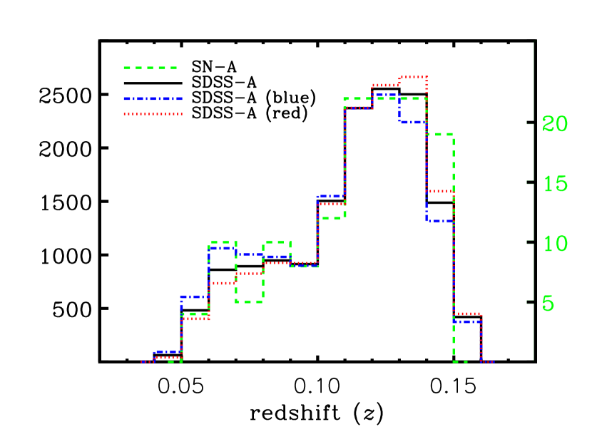
Figure 2.— The redshift distributions for the $134$ SNe Ia in sample SN–A and for the $15,000$ galaxies in sample SDSS–A. As summarized in Table 1, the SDSS–A galaxy sample is randomly chosen to match the redshift distribution of the supernovae. The red dotted and blue dashed–dotted lines show the redshift distributions for red and blue subsets of the SDSS–A sample, respectively, following the division in rest–frame $g-r$ color as given by Equation 1. Note that all histograms are normalized to have equal area. The total number of objects per bin for the SDSS–A and SN–A samples is shown by the left and right axis scales, respectively.

For the smaller SN–B sample, however, we are able to randomly select a comparison sample that matches galaxy properties such as luminosity, color, and stellar mass. From the set of $392,938$ SDSS galaxies with accurate environment measures, we draw two comparison samples: one matched to the luminosity, color, and redshift distributions of the SN hosts in sample SN–B (sample SDSS–B) and a second matched to the stellar mass, star–formation rate, and redshift distributions of the same host galaxies (sample SDSS–F).

Members of the comparison samples are drawn randomly from within 3–dimensional radial windows of $\Delta(g-r)^{2}+\Delta M_{r}^{2}+\Delta z^{2}<0.002$ and $\Delta\log(\psi)^{2}+\Delta\log({\rm M}_{*})^{2}+\Delta z^{2}<0.002$, centered on the properties of each host. The SDSS–B and SDSS–F samples are constructed from $7,500$ independent, random matches. Thus, some SDSS galaxies are duplicated in the comparison samples; however, the large size of the SDSS spectroscopic galaxy catalog ensures that duplication is minimized such that $>\!80\%$ of the comparison samples are unique, with no individual galaxy included more than $8$ times in a given comparison sample.

Figure 3 shows the relative distributions of rest–frame color, luminosity, and redshift for the galaxies in the SN–B and SDSS–B samples; by design, the distributions of these properties are well matched. Given the relatively tight relationship between the combination of rest–frame optical color and luminosity with stellar mass and star–formation rate (e.g., Kauffmann et al., 2003; Cooper et al., 2008b), we find that the distributions of stellar masses and star–formation rates for the SN–B and SDSS–B samples are also closely matched (see Figure 4). The SDSS–F sample, which is directly matched to the stellar mass and star–formation rates of the host galaxies in the SN–B sample, shows similar distributions of these galaxy properties.

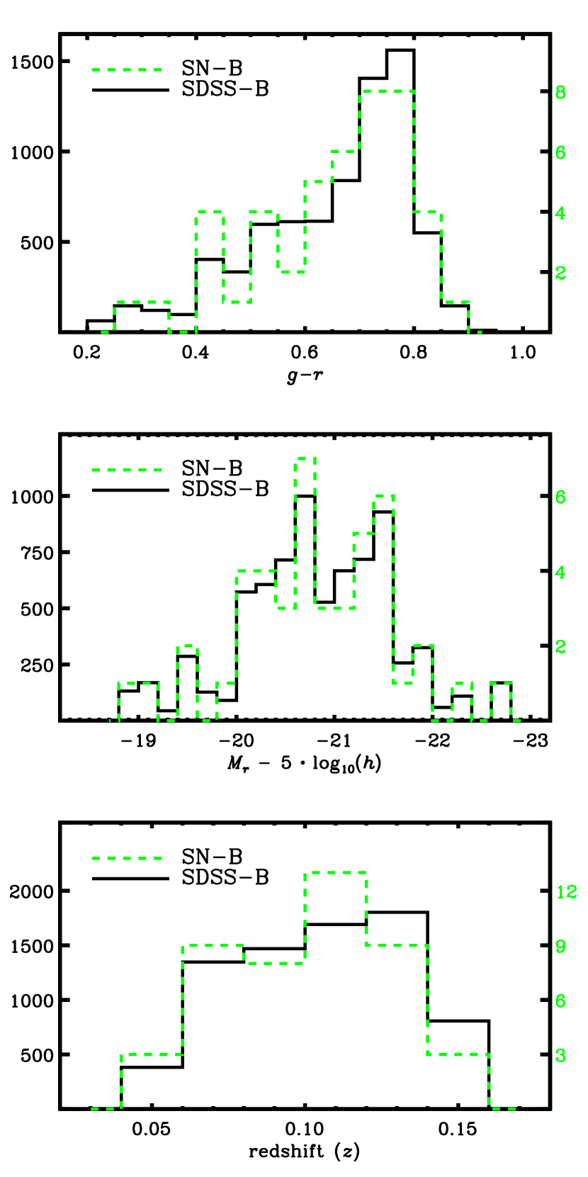
Figure 3.— The rest–frame color $(g-r)$, absolute magnitude $(M_{r})$, and redshift $(z)$ distributions for the $45$ SNe Ia host galaxies in sample SN–B and for the $7,500$ galaxies in sample SDSS–B. All histograms are normalized to have equal area. The total number of objects per bin for the SDSS–B and SN–B samples is shown by the left and right axis scales, respectively. As summarized in Table 1, the SDSS–B galaxy sample is randomly chosen to match the color, luminosity, and redshift distributions of the supernovae hosts.

Finally, we define a comparison sample (SDSS–C), selected to match the distribution of rest–frame colors, luminosities, and redshifts of the SN–C supernova sample. Recall that the SN–C sample is selected by matching the SDSS–II supernovae to the SDSS DR6 imaging catalog. Due to the lack of spectroscopic information for all of the hosts, we are unable to estimate accurate star–formation rates for the SN–C sample. The details of each of the supernova and galaxy samples is given in Table 1.

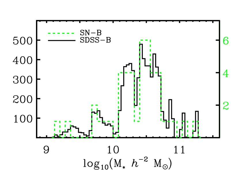
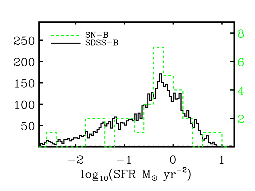
Figure 4.— The distribution of stellar masses (left) and star–formation rates (right) for the $47$ SNe Ia host galaxies in sample SN–B and for the $7,500$ galaxies in sample SDSS–B. Each histogram is normalized to have equal area, with the total number of objects per bin for the SDSS–B and SN–B samples indicated by the left and right axis scales, respectively. As summarized in Table 1, the SDSS–B galaxy sample is randomly chosen to match the color, luminosity, and redshift distributions of the supernovae hosts; however, the stellar mass and star–formation rate distributions are well matched too. This reflects the strong correlations between specific SFR and stellar mass–to–light ratio with rest–frame color.

Table 1 Descriptions of the SNe Ia and Comparison Galaxy Samples

Sample	$N_{\rm obj}$	$N_{\rm edge-cut}$	$z$ range	Brief Description
SN–A	163	134	$0.05<z<0.15$	all SNe Ia with spectra from the SDSS–II SN Survey
SDSS–A	15,000	15,000	$0.04<z<0.16$	galaxies chosen randomly to match the redshift distribution of the SN–A sample
SN–B	48	45	$0.05<z<0.15$	all SNe Ia with spectra from the SDSS–II SN Survey and with identified host galaxies within $R<25\ h^{-1}$ kpc in the SDSS spectroscopic sample, selecting the closest host in projected distance in cases of confusion
SDSS–B	7,500	7,500	$0.04<z<0.16$	galaxies chosen randomly to match the luminosity, color, and redshift distributions of the SN–B sample
SN–C	60	57	$0.05<z<0.15$	all SNe Ia with spectra from the SDSS–II SN Survey and with identified host galaxies within $R<25\ h^{-1}$ kpc in the SDSS imaging sample
SDSS–C	7,500	7,500	$0.04<z<0.16$	galaxies chosen randomly to match the luminosity, color, and redshift distributions of the SN–C sample
SN–D	48	45	$0.05<z<0.15$	all SNe Ia with spectra from the SDSS–II SN Survey and with identified host galaxies within $R<25\ h^{-1}$ kpc in the SDSS spectroscopic sample, selecting the bluest host in cases of confusion
SDSS–D	7,500	7,500	$0.04<z<0.16$	galaxies chosen randomly to match the luminosity, color, and redshift distributions of the SN–D sample
SN–E	48	45	$0.05<z<0.15$	all SNe Ia with spectra from the SDSS–II SN Survey and with identified host galaxies within $R<40\ h^{-1}$ kpc in the SDSS spectroscopic sample, selecting the closest host in projected distance in cases of confusion
SDSS–E	7,500	7,500	$0.04<z<0.16$	galaxies chosen randomly to match the luminosity, color, and redshift distributions of the SN–E sample
SDSS–F	7,500	7,500	$0.04<z<0.16$	galaxies chosen randomly to match the stellar mass, star-formation rate, and redshift distributions of the SN–B sample

Note. — We list each supernova and galaxy sample employed in the analysis, detailing the selection cut used to define the sample as well as the redshift range covered and the number of objects included before $(N_{\rm obj})$ and after $(N_{\rm edge-cut})$ removing those within $1\>h^{-1}$ comoving Mpc of a survey edge.

3. Results

In Figure 5, we show the environment distribution for the 134 supernovae in the SN–A sample in comparison to that of the SDSS–A galaxy sample. The SNe appear to be clearly biased towards lower–density environs relative to a sample of random galaxies with the same redshift distribution. Moreover, the overdensity distribution for the supernovae looks to be skewed towards low overdensities even relative to that of the blue galaxies in SDSS–A, where the blue subsample is selected following the rest–frame color division given by Equation 1.

A variety of statistical tests have been developed to determine whether two sets of data come from the same underlying distribution. We have applied two of the most powerful non–parametric tests (i.e., those which are independent of Gaussian assumptions) to our data: the one–sided Wilcoxon–Mann–Whitney U test (Mann & Whitney, 1947; Press et al., 1992; Wall & Jenkins, 2003) and the Kolmogorov–Smirnov test (Press et al., 1992; Wall & Jenkins, 2003). The result of each test is a $P$–value: the probability that a value of the U or K–S statistic equal to the observed value or more extreme would be obtained, if some “null” hypothesis holds. Throughout the remainder of this paper, results with a $P$–value below 0.05 (corresponding closely to 2$\sigma$ for a Gaussian) will be considered to be “significant”, while $P$–values below 0.01 will be classified as “highly significant”.

The Wilcoxon–Mann–Whitney U statistic is computed by ranking all elements of the two datasets together, and then comparing the mean (or total) of the ranks from each dataset. Because it relies on ranks, rather than observed values, it is highly robust to non–Gaussianity, but still has efficiency (as measured by the sample size required to reach a given error level) almost as high as the classical $t$ test for Gaussian distributions. In particular, we apply a one–sided U test, which determines the $P$–value for the null hypothesis that a specified sample is not skewed to higher values than the other sample; the obvious differences between the environments of the blue supernova hosts and blue galaxy samples (e.g., see Figure 7) make a two–sided test (for the null hypothesis that the samples have the same distribution in either sense) less appropriate. Since the test is one–sided, possible $P$–values range from $0$ to $0.5$. The Wilcoxon–Mann–Whitney (WMW) U test is particularly useful for small datasets (as we have for our SN samples) due to its insensitivity to outlying data points, its avoidance of binning, and its high efficiency.

In addition to the U test, we also employ the two–sided Kolmogorov–Smirnov (KS) test. This test quantifies differences between samples using the maximum absolute difference between the cumulative distributions of two datasets, the K–S statistic. This difference will be small for data drawn from the same distribution and large for dissimilar data; it is particularly sensitive to differences in the “core” of a distribution, but relatively insensitive to differences in tails, lending the test high robustness to non–Gaussianity. The $P$–value for the test is then the probability of obtaining the observed value of the K–S statistic, or a higher one, for the null hypothesis that we have two random datasets drawn from the same underlying distribution. If this probability is small, then the likelihood is high that the distributions of the data are not identical.

Performing a one–sided WMW U test on the overdensity measures for the SN–A and SDSS–A samples, we find that the SN–A environment distribution is skewed to smaller values of overdensity than that of the SDSS–A galaxy sample, with a $P$–value $<0.01$, i.e., there is less than a $1\%$ chance that we would observe a difference this strong if both samples were drawn from the same parent distribution. If we compare to the blue SDSS–A galaxy subsample, we still obtain $P=0.02$, which is highly significant. If instead we simply compute means and errors on the mean for the various overdensity distributions in Fig. 5, we arrive at this same general result (see Table 2). The mean overdensity, $<\log_{10}(1+\delta_{5})>$, for the SNe in sample SN–A is notably lower than the mean environment of the SDSS–A sample, with the difference significant at a $>\!3\,\sigma$ level. Relative to the mean overdensity of just the blue galaxies in the SDSS–A sample, the typical environment of the supernovae is still underdense, but with the difference only significant at a $\sim\!1\,\sigma$ level. A KS test confirms these results, indicating that the SN–A and SDSS–A environment distributions are very unlikely to have been drawn from the same parent distribution.

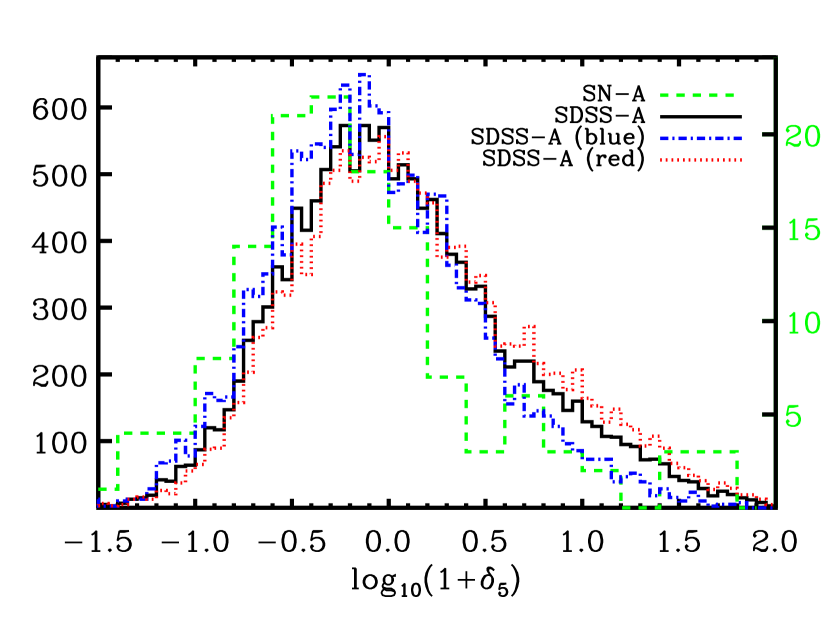
Figure 5.— We plot the distribution of overdensities for the SN–A (green dashed line) and SDSS–A (black solid line) samples. In addition, we divide the SDSS–A sample according to rest–frame $g-r$ color, following Equation 1, and plot the environment distributions for the resulting red (red dotted line) and blue (blue dashed-dotted line) subsamples. All of the histograms are normalized to have equal area, with the total number of objects per bin for the SDSS–A and SN–A samples indicated by the left and right axis scales, respectively. We find that the environment distribution for the SNe Ia in sample SN–A is skewed to lower overdensities relative to a random sample of galaxies from the SDSS with a similar redshift distribution.

The differences in the environment distributions for the SN–A and SDSS–A samples, however, are potentially only driven by differences in the properties of the two galaxy samples in concert with the underlying correlations between galaxy properties (e.g., color, morphology, etc.) and environment. For instance, a sample of galaxies chosen randomly from the SDSS DR6 galaxy catalog will undoubtedly turn out to be dominated by red galaxies; the red fraction is $60\%$ for the full SDSS sample at $0.05<z<0.15$. If we assume that the hosts of the SNe in the SN–A sample have colors that relatively closely follow the distribution of the SN–B hosts (roughly evenly divided between red and blue), then our SDSS–A sample is likely somewhat more skewed towards red galaxies than are the hosts of the SN–A sample. Since galaxy color is strongly correlated with environment, with red galaxies favoring overdense regions (e.g., Blanton et al., 2005a), the SDSS–A sample is potentially biased towards a sample of galaxies in higher–density regions, compared to the SN hosts, just because of this effect. For this reason, meaningful conclusions cannot be drawn from the analysis of the SN–A and SDSS–A samples.

The SN–B sample, which includes only those SNe with identified host galaxies in the SDSS spectroscopic sample, allows us to compare the environments of type Ia supernovae to the environments of a sample of galaxies with similar properties to those of the SN hosts, thereby avoiding the biases that weaken the utility of the larger SN–A sample. As discussed in §2.5, the SN–B sample has the additional benefit of more precise environment estimates for the supernovae (relative to the estimates for the SN–A sample), since the host galaxy redshifts have roughly $50$ times higher precision than the supernova redshifts.

In Figure 6, we show the environment distribution for the 45 SNe Ia in the SN–B sample alongside that for the SDSS–B sample, which was selected to match the color, luminosity, and redshift distributions of the 45 SN hosts. As we found for the SN–A sample, the SNe Ia in the SN–B sample appear to be more commonly found in lower–density regions relative to both the blue and the red galaxies in the SDSS–B sample. Performing a WMW U test on the overdensity measures for the SN–B and SDSS–B samples confirms that the SN–B environment distribution is distinct from that of the SDSS–B galaxy sample with a $P$–value less than $0.04$, a significant result.

By dividing the SN–B sample according to the rest–frame color of the host galaxy (again, following Equation 1), we are also able to directly compare the environment distributions for the blue and red galaxies separately. In Figure 7, we plot the distributions of overdensity measures for these subsamples selected by rest–frame color. While the distributions for the red galaxies in SN–B and SDSS–B appear to be quite similar, the overdensities for the blue SN Ia hosts are significantly skewed to lower values relative to the blue galaxies in the SDSS–B sample. Wilcoxon–Mann–Whitney U tests confirm these impressions, concluding that the overdensity measures for the blue hosts are stochastically smaller than those of the blue SDSS–B galaxies at a $>\!99\%$ level, while the distributions for the red SN–B and SDSS–B galaxy samples are indistinguishable from each other. Examining the mean overdensities, $<\log_{10}(1+\delta_{5})>$, for the respective samples confirms the result of the WMW U tests. As shown in Table 2, the mean environments for the blue samples differ at a $>\!4\,\sigma$ level, with the SN hosts being typically found in lower–density regions relative to galaxies of like color, luminosity, and redshift. Two–sided Kolmogorov–Smirnov (KS) tests similarly find that the blue hosts in the SN–B sample have an environment distribution distinct from that of the blue SDSS–B galaxies with $P<0.01$, while no significant distinction is found when comparing the environments of the red hosts in SN–B and the red galaxies in SDSS–B.

The difference between the environments of the host galaxies in the SN–B sample and the environments of like galaxies is further supported by comparing the overdensity measures for SN–B to those of the SDSS–F sample, which is a galaxy sample selected to match the stellar masses, SFRs, and redshifts of the SN–B host galaxies, rather than their colors, luminosities, and redshifts. As shown in Table 2 and Table 3, we find that the blue SN hosts in SN–B are biased to lower–density regions relative to the blue galaxies in the SDSS–F sample, with a $P$–value (or significance) similar to that found when comparing SN–B to SDSS–B.

While the environment measures for the SN–C sample are less precise than those of SN–B, due to the lack of a spectroscopic redshift for each host galaxy, we still detect a significant difference between the environment distribution of blue hosts in the SN–C sample in comparison to like galaxies in the SDSS–C sample. The mean overdensities for the blue subsamples differ at a $3.5\sigma$ level, while the typical environments of the red subsamples are indistinguishable within the uncertainties. The WMW U and KS tests support the results derived from analyzing the mean overdensities, with the environment distribution for the blue hosts distinguishable from that of a color–, luminosity–, and redshift–matched sample at $P<0.01$ and $P<0.03$, respectively.

Altogether, the primary result of analyzing the large–scale environments of samples SN–B and SN–C is that blue SN Ia host galaxies are found to be biased towards low–density environments relative to galaxies of like stellar mass, star–formation rate, and redshift. As discussed in more detail in §4, this result can be interpreted as evidence for a bias in the rate or luminosity of type Ia events in low–density regions, such that prompt Ia events are more numerous or more luminous in underdense environs.

One of the most striking features of the environment distribution for the blue hosts in SN–B, as shown in Fig. 6, is the complete lack of blue host galaxies in high–density regions. All of the supernovae in star–forming systems are found in overdensities of $\log_{10}(1+\delta_{5})<0.14$, while the blue comparison galaxies in the SDSS–B sample span the full range of overdensities. To test the significance of this sharp cut–off in overdensity, we draw $100,000$ random subsets of $20$ galaxies each from the blue SDSS–B sample. Of these $100,000$ subsamples, we find that less than $0.1\%$ display sharp cut–offs in their environment distribution such that all $20$ galaxies reside in overdensities of $\log_{10}(1+\delta_{5})<0.15$. This analysis further supports the conclusion that the SN Ia rate or luminosity is elevated in low–density environments (relative to more overdense environs) among star–forming galaxies.

We test the strength (or depth) of this cut–off in overdensity by measuring how much of an increase in the type Ia rate in low–density environments is needed to make the observed cut–off at $\log_{10}(1+\delta_{5})=0.15$ statistically likely to occur. To do this, we select the $3244$ random blue galaxies in the SDSS–B sample, which by design match the rest–frame color, absolute magnitude, and redshift distributions of the blue SN Ia hosts in sample SN–B. From this parent population, we then draw $100,000$ independent samples of $20$ random galaxies with the likelihood of drawing an object in a low–density $(\log_{10}(1+\delta_{5})<0.15)$ environment forced to be $2\times$ greater than that of a galaxy in a high–density $(\log_{10}(1+\delta_{5})\geq 0.15)$ environment. The division between the underdense and overdense regimes is selected to be $\log_{10}(1+\delta_{5})=0.15$, so as to maximize the probability of seeing an apparent cut–off. We repeat this exercise while varying the degree to which the SN rate increases in the underdense regime (e.g., $3\times$ and $4\times$ greater, etc.).

We find that to have a $1\%$, $5\%$, or $32\%$ probability of observing a cut–off at $\log_{10}(1+\delta_{5})=0.15$ would require an increase in the SN Ia rate in low–density environments at the level of $>\!1.5\times$, $2.5\times$, and $7\times$, respectively. Thus, a SN Ia rate $\gtrsim\!2\times$ higher within star–forming galaxies in low–density environments (relative to those in more overdense regions) is likely required to produce the observed cut–off in the environment distribution among the blue SN host galaxy population.

From this statistical analysis, we have determined the probability of observing so strong a strong cut–off in environment, given a SN rate in high–density environs which is $R$ times that in low–density regions, as a function of $R$. From this, we can determine the Bayesian equivalent of a 95% confidence interval, a 95% credible interval, as this will be the region containing 95% of the posterior probability. Bayes’ theorem (Press et al., 1992; Wall & Jenkins, 2003) shows that this posterior probability will be proportional to the probability of obtaining a cut–off as strong as observed (or stronger) for a given $R$ — the likelihood — multiplied by the probability distribution we would assign to $R$ in the absence of any measurements — a prior. Based on this analysis, we conclude that there is $95\%$ probability that $R<0.38$; i.e., that the SN Ia rate is less than $0.38$ times as large in the high–density regime ($\log_{10}(1+\delta_{5})\geq 0.15$) as at lower densities, assuming a flat prior probability distribution for $R$, a conventional zero–information prior for a parameter with some characteristic scale (e.g., $R=1$). If we instead adopt a prior with uniform probability for all intervals of $\log(R)$ (i.e., $P(R)=1/R$), we would find that there would be only a $5\%$ probability that $R>0.12$. Finally, even with a prior as extreme as $P(R)=R$, which favors $R>1$, we find that there is $95\%$ probability that $R<0.66$; an equal SN rate in high– and low–density regions ($R=1$) is strongly ruled out by our analysis.

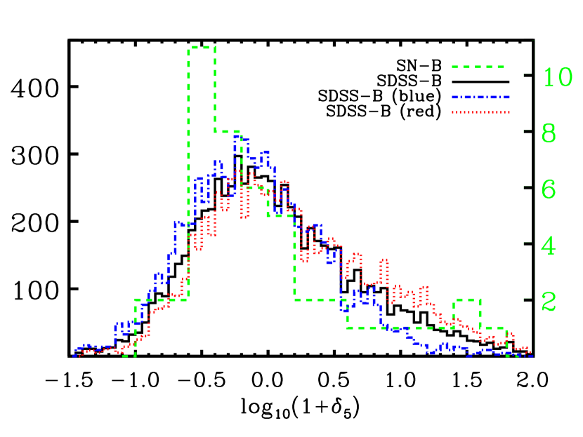
Figure 6.— We plot the distribution of overdensities for the SN–B (green dashed line) and SDSS–B (black solid line) samples. In addition, we divide the SDSS–B sample according to rest–frame $g-r$ color, following Equation 1, and plot the environment distributions for those red (red dotted line) and blue (blue dashed-dotted line) subsamples. All of the histograms are normalized to have equal area, with the total number of objects per bin for the SDSS–B and SN–B samples indicated by the left and right axis scales, respectively. We find that the environment distribution for the type Ia SN hosts in the SN–B sample is skewed to lower overdensities relative to a randomly–selected sample of galaxies with matching luminosity, color, and redshift distributions.

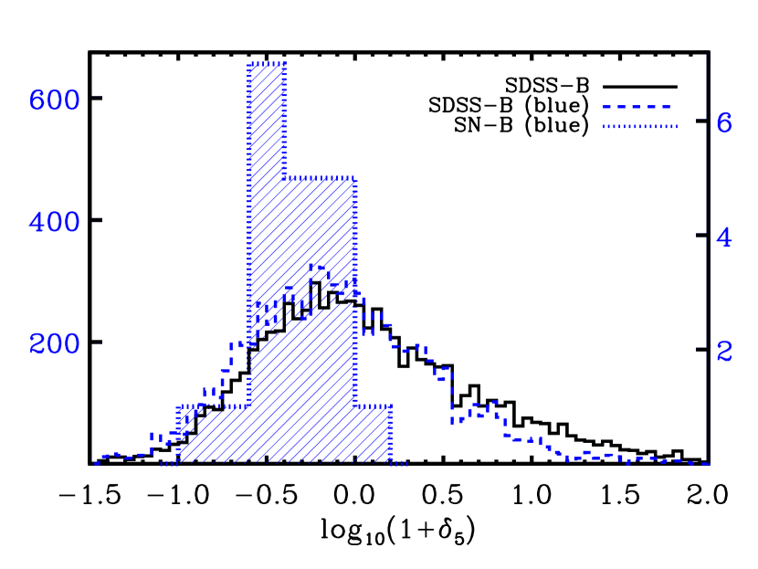
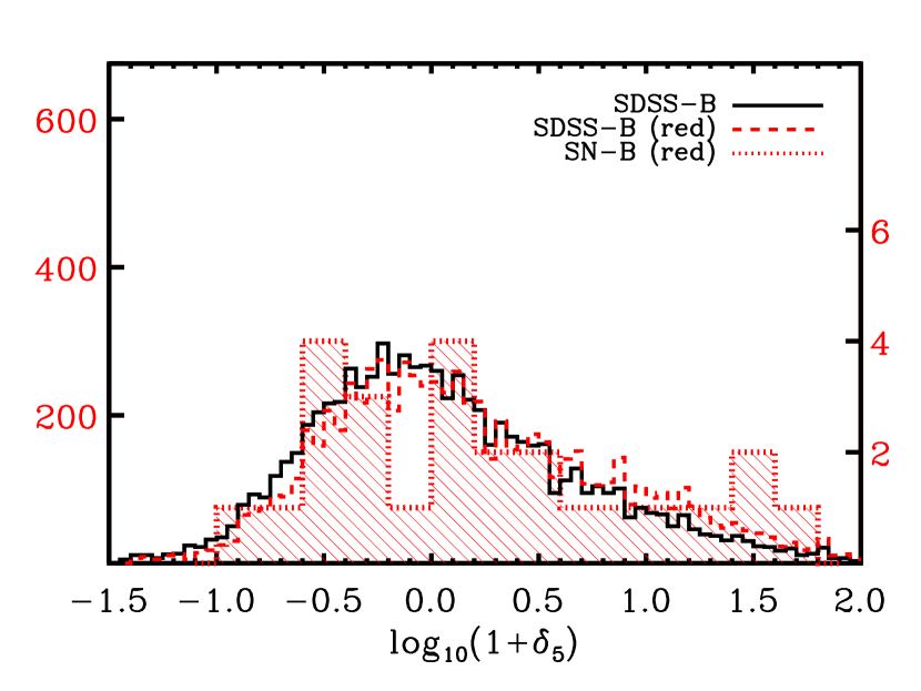
Figure 7.— We plot the distribution of overdensities for the blue (left) and red (right) galaxies in the SN–B and SDSS–B samples. All of the histograms are normalized to have equal area. The total number of objects per bin for the blue or red SDSS–B and SN–B samples is shown by the left and right axis scales, respectively. We find that the environment distribution for the blue type Ia SN hosts in the SN–B sample is skewed to lower overdensities relative to a sample of blue galaxies with similar luminosity, color, and redshift distributions.

Table 2 Summary of Mean Overdensities

Sample	$<\log_{10}(1+\delta_{5})>$	$\sigma_{<\log_{10}(1+\delta_{5})>}$	Sample	$<\log_{10}(1+\delta_{5})>$	$\sigma_{<\log_{10}(1+\delta_{5})>}$
			SDSS–A	0.070	0.005
SN–A	-0.132	0.059	SDSS–A [blue]	-0.073	0.007
			SDSS–A [red]	0.160	0.006
SN–B	-0.023	0.098	SDSS–B	0.079	0.007
SN–B [blue]	-0.345	0.053	SDSS–B [blue]	-0.083	0.009
SN–B [red]	0.235	0.153	SDSS–B [red]	0.196	0.009
SN–C	0.011	0.094	SDSS–C	0.100	0.009
SN–C [blue]	-0.338	0.064	SDSS–C [blue]	-0.077	0.012
SN–C [red]	0.248	0.138	SDSS–C [red]	0.219	0.012
SN–D	0.009	0.101	SDSS–D	0.082	0.007
SN–D [blue]	-0.171	0.130	SDSS–D [blue]	-0.090	0.009
SN–D [red]	0.174	0.146	SDSS–D [red]	0.229	0.010
SN–E	-0.017	0.096	SDSS–E	0.087	0.007
SN–E [blue]	-0.317	0.058	SDSS–E [blue]	-0.074	0.009
SN–E [red]	0.235	0.153	SDSS–E [red]	0.216	0.010
			SDSS–F	0.077	0.007
			SDSS–F [blue]	-0.062	0.009
			SDSS–F [red]	0.170	0.009

Note. — The mean and the error on the mean of the overdensity distributions for the various SNe and galaxy samples.

Table 3 Summary of Statistical Tests

Samples	$P_{{\rm WMW}}$	$P_{{\rm KS}}$
SN–A/SDSS–A	$5.5\times 10^{-6}$	$6.8\times 10^{-5}$
SN–A/SDSS–A [blue]	0.011	0.030
SN–B/SDSS–B [blue]	0.005	0.006
SN–B/SDSS–B [red]	0.499	0.846
SN–C/SDSS–C [blue]	0.006	0.024
SN–C/SDSS–C [red]	0.479	0.632
SN–D/SDSS–D [blue]	0.068	0.057
SN–D/SDSS–D [red]	0.336	0.639
SN–E/SDSS–E [blue]	0.011	0.018
SN–E/SDSS–E [red]	0.479	0.850
SN–B/SDSS–F [blue]	0.002	0.005
SN–B/SDSS–F [red]	0.435	0.811

Note. — We tabulate the $P$–values, $P_{\rm WMW}$ and $P_{\rm KS}$, from comparing the environment values in the listed samples, using the one–sided Wilcoxon–Mann–Whitney (WMW) U test and the two–sided Kolmogorov–Smirnov (KS) test. As discussed in §3, smaller values indicate a lower probability that the observed differences in the samples will occur by chance if they are selected from the same underlying parent distribution. Note that, as a one–sided test, $P_{\rm WMW}$ has a maximum value of $0.5$.

4. Discussion

In §3, we show that the SNe Ia in blue host galaxies occur preferentially in low–density environments relative to galaxies of like color and luminosity (or like stellar mass and star–formation rate). For the type Ia events in red hosts, however, we find no significant difference between the environments of the host galaxies and the environments of comparison galaxy samples. In the following subsections, we examine how these results compare to the results of related studies in the literature. We also investigate potential selection effects, which could bias our supernova and galaxy samples, and finally we discuss the implications of our results in terms of the currently–unknown SN Ia progenitor population.

4.1. Comparison to Previous Work

Recent analyses have reached a variety of conclusions regarding the dependence of the SN Ia rate on environment. Using angular cross–correlation techniques on data from the SNLS, Carlberg et al. (2008) found that supernova hosts at $0.2<z<0.9$ are more strongly clustered than a sample of field galaxies selected to have the same redshift and ($i$–band) brightness distributions as the hosts. However, inaccurate photometric redshifts could, by overbroadening the measured galaxy redshift distribution, dilute the measured angular–clustering strength for the galaxy sample relative to that of the supernovae, for which spectroscopic redshifts were obtained. Furthermore, the comparison sample is not selected to match the stellar mass, rest–frame color, or SFR distributions of the host galaxies. Thus, this result could also be attributed to the dependence of the SN Ia rate on galaxy properties, where the SN Ia rate increases with stellar mass and star–formation rate, and to the dependence of galaxy properties on environment, where more massive galaxies favor overdense environs. In fact, when weighting their field galaxy sample by stellar mass and star–formation rate, Carlberg et al. (2008) show that the clustering of the type Ia supernova hosts and field galaxies in the SNLS are in good agreement. A parallel analysis of data drawn from the SNLS by Graham et al. (2008), focusing on SNe Ia identified within galaxy clusters at intermediate redshift, found no significant difference between the SN Ia rate in clusters from that in field ellipticals. However, their supernova sample is quite small (only three probable cluster Ia events) and the results are dominated by statistical uncertainties.

Studying supernovae in the local $(z<0.2)$ Universe, Sharon et al. (2007) found the type Ia rate in nearby clusters to be roughly consistent with estimates of the SN Ia rate in local elliptical galaxies; this work, however, was based on a sample of only six cluster supernovae and thus yielded very large uncertainties in the measured cluster type Ia rate. A more recent analysis of data in nearby ($z<0.04$) clusters by Mannucci et al. (2008) arrived at a very different result, finding that the SN Ia rate (per unit mass) is more than 3 times higher in cluster ellipticals relative to field ellipticals, using a sample of 11 cluster and 5 field type Ia events; an identical SN rate in both samples is excluded with $P=0.02$. In their analysis, Mannucci et al. (2008) compare the rate within galaxies of like mass and morphology, attempting to remove the known correlations between galaxy properties and environment. For this reason, and the similarity in redshift range probed, the Mannucci et al. (2008) study provides the most significant and relevant comparison to our results.

In particular, the environment–dependent rates of Mannucci et al. (2008) are most closely connected to our results regarding the environments of red SN Ia hosts. In contrast to the results of Mannucci et al. (2008), we find no significant trend such that supernovae occur more often in overdense regions; within our SDSS samples, the environment distribution for the subset of red hosts is indistinguishable (within the uncertainties) from that of the samples of red comparison galaxies (see Table 2 and Table 3). However, our results regarding the environments of red host galaxies have large statistical uncertainties associated with them, making any strong statement about the environment dependence of the type Ia rate in red (or elliptical) hosts impossible.

To investigate any potential discrepancy between our results and those of Mannucci et al. (2008), we attempt to test the likelihood that we would have detected the Mannucci et al. (2008) result of a $>\!3\times$ higher SN Ia rate in cluster ellipticals relative to field ellipticals, given our sample size of 25 red SN Ia hosts in SN–B. From the SDSS–B galaxy sample, we select the $4256$ random red galaxies which match the rest–frame $g-r$ color, absolute $r$–band magnitude, and redshift distributions of the red SN Ia hosts in sample SN–B. From this parent population, we then draw $5000$ independent samples of $25$ random galaxies with the likelihood of drawing an object in a high–density $(\log_{10}(1+\delta_{5})>1)$ environ forced to be $3\times$ greater than that of a galaxy in a low–density $(\log_{10}(1+\delta_{5})\leq 1)$ environ. For each realization, we compare the distribution of environments for the $25$ mock SN hosts to the full sample of red galaxies in the SDSS–B sample, using the Wilcoxon–Mann–Whitney U and Kolmogorov–Smirnov statistical tests. Finally, this mock sample–selection analysis is repeated with galaxies in high–density environments selected at $1\times$, $2\times$, and $4\times$ the rate of galaxies in low–density regions.

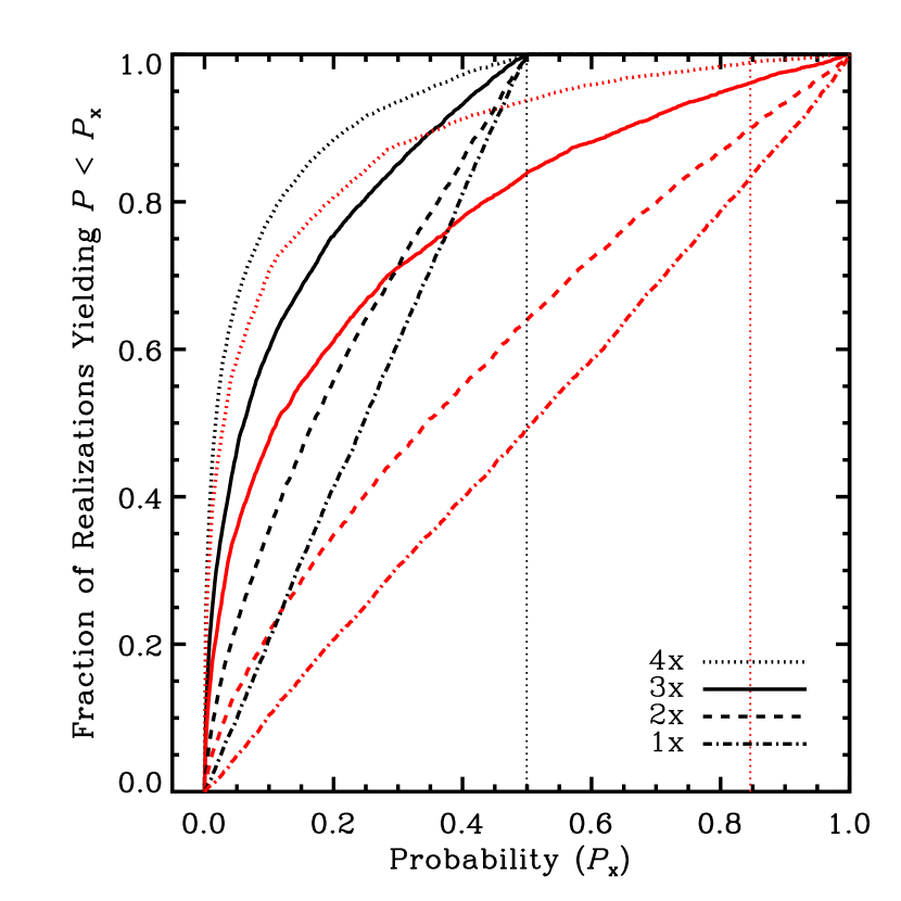
Figure 8.— For $5000$ mock realizations of a SN Ia rate $3\times$ higher in high–density than in low–density environments, we plot the percentage of realizations that yield a one–sided Wilcoxon–Mann–Whitney (WMW) probability less than $P_{x}$ (solid black line) and a two–sided Kolmogorov–Smirnov (KS) probability less than $P_{x}$ (solid red line). The black dotted, dashed, and dashed-dotted lines correspond to mock realizations simulating a SN Ia rate in high-density regions $4\times$, $2\times$, and $1\times$ that in low–density environs, respectively. Note that the black lines reach a fraction of unity at a probability ($P_{x}$) of $0.5$ since they correspond to the one–sided WMW test, while the red lines saturate at $P_{x}=1$ since they correspond to the two–sided KS test. The black and red vertical dotted lines give the WMW and KS probabilities, respectively, computed from a comparison of the environments of red galaxies in the SN–B and SDSS–B samples (see Table 3).

As shown in Figure 8, in only $\sim 50\%$ of the mock realizations with a $3\times$ higher likelihood of SNe occurring in dense environs, would we have rejected the hypothesis that the environments of SN hosts are on average no more overdense than that of the SDSS–B red galaxy sample with $P<0.05$. The likelihood that we would have detected a difference in the typical environment becomes even smaller when we assume a SN Ia rate that is only $2\times$ higher in dense environs; in this case, the WMW test $P$–value is $<\!0.05$ in $25\%$ of the mock realizations.

When we apply the two–sided KS test, we find similar results; for the majority ($>\!60\%$ and $>\!85\%$) of mock realizations, we would not have detected a significant difference in the environment distributions at a $P>0.05$ significance level, assuming a SN Ia rate $3\times$ and $2\times$ higher in overdense regions, respectively. Thus, while our analysis of type Ia supernovae in red SDSS hosts does not support the conclusions of Mannucci et al. (2008), our results are not in direct conflict either, given the large uncertainties in both results. With that said, the high WMW and KS $P$–values computed from a comparison of the environments for the red SN–B and SDSS–B galaxies (see Table 3) occur only rarely in our simulated galaxy samples and thus favor a SN Ia rate in cluster ellipticals more in line with that of field ellipticals, at the low end of the possible range given by Mannucci et al. (2008).

While the Mannucci et al. (2008) work has a sample size roughly double that of Sharon et al. (2007), the uncertainties in their measured SN Ia rates are still quite large, such that the field and cluster rates are only different at a $2.1\sigma$ level, thereby leaving much uncertainty in the dependence of the type Ia rate on environment within early–type galaxies.

4.2. Potential Selection Effects

While the SDSS–II Supernova Survey includes $>\!100$ SNe Ia with spectroscopic follow–up in the redshift range $0.05<z<0.15$, less than half of the total sample is successfully matched to a host galaxy in the SDSS DR6 spectroscopic sample. Given the large number of unmatched supernovae, it is important to understand any potential biases that could arise from the particular method adopted to identify host galaxies. For example, our observation that SNe Ia in blue galaxies are biased towards low–density environments could naturally arise from employing an algorithm to select host galaxies that is for some reason biased against finding hosts in overdense regions (e.g., groups or clusters). Given the strong correlations between environment and galaxy properties, it is also critical to understand any aspect of the host–identification methodology that could be biased towards identifying hosts of a particular galaxy color, luminosity, etc.

To test the sensitivity of our results to the particularities of the host–identification algorithm, we define two additional SN samples, SN–D and SN–E (see Table 1 for sample definitions). The SN–D sample is selected to test for any bias in the SN–B sample towards SNe being preferentially matched to red host galaxies. For the vast majority of SNe in the SN–B sample, only one possible host galaxy is found within the cylindrical search window (see §2.3 for the details of the SN–B matching algorithm). However, for three SNe, multiple host galaxies are identified within the SDSS spectroscopic data set. In Figure 1, we mark the location of these possible, alternate (“secondary”) host galaxies using magenta stars, with dotted lines connecting them to the location of the “primary” host, as defined in the SN–B sample.

While the choice of the host galaxy in these ambiguous cases does not significantly impact the measured environment of the SNe, the location of the host in color–magnitude space directly affects whether the host is classified as “blue” or “red” in our color cuts and affects the composition of the comparison galaxy sample (SDSS–B). Confusion among hosts is likely to be more common in overdense regions, which could cause a small bias in the measured distribution of supernova environments when divided into blue and red subsamples.

To test the robustness of our results to the ambiguity in the host identification, we apply a Murphy’s Law approach, where if anything can go wrong to bias our SN–B sample, then it will. In the ambiguous cases, we correspondingly match the SNe to the bluest host according to rest–frame $g-r$ color. Given the potential host galaxies, this creates the sample of SN hosts (SN–D) with the highest possible mean density among blue host galaxies (see Table 2). Even in this extreme (and somewhat unlikely) scenario, we still find that the distribution of environments for the blue SN hosts in sample SN–D is distinct from that of a corresponding sample of galaxies chosen to match in color, luminosity, and redshift (sample SDSS–D), with the difference significant at a $>\!94\%$, following a two–sided KS test.

Another aspect of the host–identification methodology that might lead to a bias against identifying hosts for SNe in dense regions is the size of the cylindrical aperture used to search for possible host galaxies. If this aperture is too small, then the sample could be biased against including SNe in galaxies of greater physical size. Massive galaxies, which are inclined to reside in overdense environments (e.g., Cooper et al., 2008a), also tend to have larger sizes (Shen et al., 2003) and larger velocity dispersions (Faber & Jackson, 1976; Djorgovski & Davis, 1987), which potentially could lead to SNe occurring at projected and velocity separations outside of the windows used to define the hosts in SN–B.

Recognizing these correlations between galaxy size, velocity dispersion, and environment, we alternatively identify a host galaxy sample (SN–E) using a projected, radial window of $40\>h^{-1}$ kpc (physical) to identify potential hosts on the plane of the sky in conjunction with a velocity window of $\Delta v=5000\ {\rm km}\ {\rm s}^{-1}$ along the line of sight, both $\sim\!60\%$ larger than the windows of $25\>h^{-1}$ kpc and $\Delta v=3000\ {\rm km}\ {\rm s}^{-1}$ used to define the hosts in sample SN–B. Like when defining sample SN–B, when multiple potential hosts are identified within this window, the galaxy closest in projected distance is taken as the host. Using these larger radial and line–of–sight search windows, only one additional supernovae is matched to a host (relative to the number of hosts identified in SN–B); however, the percentage of SNe unambiguously matched to a host declines slightly from 92% to 88%. Thus, we conclude that our SN–B sample is not significantly biased against SNe occurring in more massive galaxies.

A final potential selection effect associated with the identification of SN hosts is the possibility that matching to the SDSS spectroscopic galaxy sample is biased against matching SNe to hosts in rich environments due to fiber collisions. Our SN–A and SN–C samples are specifically designed to test for such an effect. By matching directly to the imaging catalog, SN–C avoids any bias associated with the allocation of fibers in the spectroscopic component of the SDSS. We find that the general results obtained by analyzing the SN–B sample are supported by the analysis of the SN–C sample. Thus, we conclude that our results are likely robust to any bias associated with allocation of SDSS fibers in overdense regions. As shown by Cooper et al. (2005) and Gerke et al. (2005), dense regions on the sky do not always translate into dense regions in redshift space.

Looking beyond selection effects that might bias the host–identification process, we also examine the possibility that our supernova samples are biased against bulge–dominated systems. Given the higher surface brightness of bulges, relative to galactic disks, it can be more difficult to obtain spectroscopic follow–up data for a supernova near the bulge of a galaxy. For galaxies with larger bulges, this problem is obviously greater. Moreover, observations of local type Ia SNe find correlations between the light–curve decline rate and the peak luminosity with morphology, such that late–type galaxies host brighter SNe Ia (e.g., Hamuy et al., 1995, 1996; Gallagher et al., 2005). Thus, given the correlation between morphology and environment, where the bulge–dominated fraction increases with local density, our observed deficit of supernovae in high–density environments within the star–forming population and lack of an increase in the type Ia rate within cluster red–sequence members could both be attributed to such a morphology bias.

To test for this selection effect, we compare the morphology distribution of our host galaxies in the SN–B sample to that of the galaxies in the SDSS–B comparison sample. As a tracer of morphology, we utilize the Sérsic indices as measured for SDSS galaxies by Blanton et al. (2003b, 2005a). While the Sérsic index is a measure of morphology derived from the fit of only a single component to the galaxy’s radial profile (e.g., versus bulge-disc decomposition), we find no significant difference in the morphologies of our supernova hosts relative to the morphologies of the comparison galaxies.

In much the same way that it can be difficult to detect a supernova superimposed on a bulge relative to a disk, follow–up spectroscopy of candidate events (used to confirm the supernova type) is also affected by the relative brightness of the host galaxy; spectroscopic observations of supernovae in brighter hosts are more difficult due to contamination of the supernova spectrum by emission from the host galaxy. Any incompleteness in our sample that is dependent on apparent magnitude, however, is effectively controlled for in our samples by matching the comparison galaxy samples (e.g., SDSS–B) to the supernova host samples (e.g., SN–B) according to color, luminosity, and redshift. By matching both luminosity and redshift, the samples being compared also have the same brightness. For the very same reason, our analysis is insensitive to any incompleteness in the SDSS spectroscopic catalog that may result from failing to obtain redshifts for fainter galaxies.

Finally, we test the robustness of our results to the particularities of our adopted color division between blue and red populations. To do this, we shift the color cut given in Equation 1 by $\pm 0.04$ magnitudes in rest–frame $g-r$ color, which results in changes in the blue and red components of the SN–B supernova sample of $\pm 3$ supernovae. With these changes in the subsample definitions, our results regarding the environments of blue host galaxies remain “highly significant” (i.e., $P<0.01$). Furthermore, even when shifting the color cut by as much as $0.1$ magnitudes, the WMW U and KS tests indicate that the blue supernova host galaxies populate a significantly (i.e., $P\lesssim 0.05$) distinct distribution of environments from the blue comparison galaxies in the SDSS–B sample.

4.3. Supernova Ia Progenitors

As discussed in §1, observational studies of nearby and distant supernovae have supported the definition of two components to the type Ia supernova rate, a “prompt” and a “delayed” component. However, there is no current observational evidence that indicates two distinct progenitor channels associated with the two components of the type Ia rate. With that said, recent theoretical analyses have found difficulty reconciling observations with models in which both the “prompt” and “delayed” Ia components result from single–degenerate events, where a carbon–oxygen WD accretes matter from a non–degenerate, companion star (e.g., Yungelson & Livio, 2000; Greggio, 2005; Pritchet et al., 2008). Allowing for the possibility of double–degenerate scenarios, in which two WDs are drawn together via angular momentum losses resulting from gravitational radiation (Iben & Tutukov, 1984; Webbink, 1984), some success has been found at predicting observed SN rates as well as the chemical enrichment of local galaxies (Greggio, 2005; Matteucci et al., 2006; Greggio et al., 2008).

If the two components of the type Ia rate are somehow comprised of single– and double–degenerate events, then the “prompt” component is likely primarily driven by single–degenerate events, due to their shorter minimum timescale for occurrence. That is, single–degenerate events are favored for the “prompt” component, since the minimum timescale between formation of the progenitor star and occurrence of the supernova is on the order of the lifetime of a $8{\rm M}_{\sun}$ star (i.e., $\sim\!30$ Myr), while the minimum timescale for occurrence of a double–degenerate event is considerably longer ($\sim\!1$ Gyr, Greggio, 2005). Thus, our results suggest that single–degenerate events are favored (or are more luminous) in low–density environs, given the assumptions detailed above.

Now, while physical mechanisms such as galaxy mergers or harassment are more common in high–density regions such as groups and clusters, it is difficult to suggest a physical mechanism specific to low–density environs that would directly impact the evolution of stellar populations and influence the SN Ia rate or luminosity (e.g., by raising the binary fraction so as to produce more type Ia events). It is seemingly more likely that environment is strongly correlated with a galaxy property that traces differences in stellar populations, such as stellar or gas–phase metallicity or stellar age. In the following section (§4.4), we discuss this issue in more detail.

4.4. The Role of Metallicity

As discussed in detail in §3, we find that blue SN Ia host galaxies are only seen in comparatively low–density regions, suggesting that prompt supernovae Ia occur (or are found) preferentially in underdense environs or that they are somehow suppressed in the high–density regime. However, there is little physical motivation for connecting large–scale environment–specific processes (e.g., mergers, strangulation, etc.) with the generation or suppression of type Ia supernovae. A potentially interesting, though currently poorly unconstrained, possibility could be that merger–induced star formation has somewhat different properties (e.g., a different initial mass function) than typical star formation (e.g., due to higher gas densities). The prevalence of mergers in environments such as galaxy groups could thus be associated with an environment dependence to the prompt Ia rate or luminosity.

Another possibility could be the suppression of SNe within galaxies in clusters due to ram–pressure stripping, where the (metal–poor) outskirts of systems are preferentially confiscated by the IGM. The stripped gas and stars would then contribute to the intracluster light and result in intracluster (i.e., intergalactic) supernovae (Gal-Yam et al., 2003; Maoz et al., 2005). Such supernovae could be missed by narrow–field supernova searches that target individual galaxies in clusters rather than large fields (e.g., Cappellaro et al., 1999). The imaging data from the SDSS–II Supernova Survey, however, covers a large and nearly continuous field, such that any intracluster SNe would be included in the supernova sample. Still, an intracluster SN would be less likely to be matched to a host galaxy, thereby mimicking a suppression of SNe within galaxies in overdense regions. Given the large uncertainties in the cluster SN Ia rate and in the relative contribution from intracluster events (Gal-Yam et al., 2003), the role of such supernovae remains largely unknown. With that said, the relatively low concentration of blue galaxies in local clusters helps to minimize the impact of intracluster events on our results, as related to the preferential occurrence of SNe Ia in blue host galaxies in underdense environs.

Alternatively, it could be the case that environment is correlated with a galaxy property or properties, for which we did not control in our analysis. A correlation between a given physical property and environment would cause the overdensities about our SN host galaxies to be skewed relative to the comparison sample, if supernova host galaxies are a (relatively) biased tracer of that galaxy property. One likely galaxy characteristic to consider is metallicity.

The metal abundance of a galaxy is often quantified in two ways: [1] by measuring the metal abundance in the interstellar medium (the gas–phase metallicity) and [2] by assessing the amount of metals locked up in the stellar population (the stellar metallicity). The gas–phase metallicity is a product of the recent ($<\!1$ Gyr) accretion and star–formation history of the galaxy (Finlator & Davé, 2008). In contrast, the stellar metallicity, which is commonly inferred from fits to stellar absorption features in optical spectra, traces the metals locked up in the old stellar population. Thus, stellar metallicity is a tracer of the integrated star–formation history and a measure of the gas–phase metallicity in the galaxy when the bulk of the stars formed. Here, we investigate the potential role of both stellar and gas–phase metallicity in biasing our supernova samples in star–forming galaxies towards underdense environments.

To study the potential role of stellar metallicity in our results, we employ the measurements of Gallazzi et al. (2005), which are based on model fits to spectral absorption features in the SDSS DR4 spectra. The measurements are sensitive to the signal–to–noise ratio of the spectrum (see Table 1 of Gallazzi et al., 2005), which limits our ability to directly constrain the stellar metallicities of the SN hosts. More than half of the SNe in our sample are at $z>0.1$, which means that the host galaxies tend to be relatively faint in the $r$–band (less than $25\%$ of the SNe have an $r$–band magnitude $<\!16.5$) and the derived metallicity values are highly uncertain. For this reason, we are unable to make any meaningful statements about the stellar metallicity values of the hosts relative to the comparison galaxy samples.

However, we are able to study the relationship between stellar metallicity, $Z$, and environment for the general SDSS galaxy population, which allows us to understand how our results regarding the environments of type Ia hosts could be understood in terms of a stellar metallicity bias. In the Appendix, we investigate in detail the relationship between metallicity and environment for three magnitude–limited samples drawn from the Gallazzi et al. (2005) catalog. As shown in Figure 11, we find a significant correlation such that galaxies with more metal–rich stellar populations typically reside in more overdense environs. Furthermore, this general correlation persists when focusing on just those galaxies that reside on the blue cloud (following Equation 1); although, the trend is considerably weaker.

A corresponding relationship between gas–phase metallicity and environment was recently published by Cooper et al. (2008a); studying star–forming galaxies in the SDSS DR4, they found a significant correlation between average gas–phase metallicity and local galaxy density, such that more metal–rich galaxies favor regions of higher overdensity. Along the blue cloud, this metallicity–density relation is comparable in strength to the well–known color–density relation. Moreover, Cooper et al. (2008a) show that metallicity has a relationship with environment separate from that observed with color and luminosity (or with stellar mass). Gas–phase metallicity is somewhat unique in this regard, as other galaxy properties (e.g., surface brightness, Sérsic index, or stellar mass) that are strongly correlated with overdensity do not show a relationship with environment separate from that observed with color and luminosity (Blanton et al., 2005a; Cooper et al., 2008a).

In order for the results in §3 to be due to either of these observed correlations between environment and metallicity (either stellar or gas–phase), the blue SN host galaxies must be biased towards lower stellar or gas–phase metallicities than the comparison galaxy samples. As discussed above, however, we are unable to directly test for any potential bias in our supernova samples, due to the lack of metallicity information (both stellar and gas–phase) for the majority of the hosts. Given the low signal–to–noise of the SDSS spectra, reliable metallicity measures are not feasible. Without direct constraints on the metallicities of the SDSS host galaxies, our results regarding the environments of SNe Ia in star–forming galaxies could still (at least partially) be understood in terms of a metallicity effect if the luminosity or the rate of type Ia events depends on metallicity, such that intrinsically brighter supernovae arise from more metal–poor progenitors or such that the type Ia rate is elevated in metal–poor host galaxies.

However, recent observational work by Howell et al. (2008), studying SNe Ia in a relatively large sample $(>\!100)$ of star–forming and quiescent host galaxies at $z\leq 0.75$, suggests that variation in gas–phase metallicity only accounts for a small portion $(<\!10\%)$ of the measured dispersion in type Ia luminosities (see Figures 5, 7, and 11 of Howell et al., 2008). A variety of previous studies (e.g., Hamuy et al., 2000; Ivanov et al., 2000; Gallagher et al., 2005), using both gas–phase and stellar metallicity estimates, also found no significant evidence for a correlation between metallicity and the properties of SNe Ia. With that said, whether low–metallicity stars might yield more luminous type Ia events is still a relatively poorly constrained question. For example, the gas–phase metallicity estimates employed by Howell et al. (2008) are derived from using measurements of the hosts’ stellar masses to estimate the oxygen abundances according to the median mass–metallicity relation for nearby star–forming systems (Tremonti et al., 2004). This method is applied even to those systems thought to be quiescent and are thus not included in the analysis of Tremonti et al. (2004). Future observations, yielding direct oxygen abundance measurements, are needed to better determine the relationship between metallicity and type Ia luminosity.

While the luminosities of type Ia SNe show no significant correlation with metallicity, our observations of supernova environments could also be explained by an increase in the SN Ia rate in metal–poor hosts. From an observational standpoint, the dependence of the type Ia rate on host metallicity remains unconstrained, with current supernova samples including precision metallicity measurements for only a small portion of the host population. Still, recent observational studies show that a considerable number of type Ia supernovae have been found in low–metallicity galaxies (Strolger et al., 2002; Prieto et al., 2008). On the other hand, observations of type Ia supernovae in nearby, star–forming galaxies with significantly enriched interstellar media are evidence that the SN Ia rate is not zero in the metal–rich regime (e.g., Gallagher et al., 2005).

In addition, theoretical models of supernovae suggest that the type Ia rate depends significantly on metallicity, such that the rate is lower in galaxies with lower metallicities (e.g., Tornambe & Matteucci, 1986; Hachisu et al., 1996; Kobayashi et al., 1998, 2000, but also see Umeda et al. 1999b). This theoretical metallicity effect, however, works counter to that which would explain our observations of supernova and galaxy environments, making our results regarding the environments of type Ia SNe in star–forming systems even more remarkable. With that said, the theoretical models are generally constrained on a limited basis, being forced to match observations of chemical evolution in the solar neighborhood.

In spite of the theoretical predictions regarding the dependence of the SN Ia rate on metallicity, our results appear to be most easily understood in terms of a gas–phase metallicity effect, where prompt SNe Ia preferentially arise from metal–poor progenitors. In particular, the sharp cut–off in the observed distribution of environments for SNe Ia in blue hosts could be the result of a sharp feature in the metallicity distribution of the prompt SNe Ia progenitor population, such that prompt type Ia events rarely result from the evolution of relatively metal–rich stars.

This picture is supported (though circumstantially) by several key points. First, the bias in the galaxy environment distribution for SNe Ia in star–forming systems towards underdense regions is likely attributable to the prompt (versus delayed) component of the type Ia population, since delayed SNe are seen in both star–forming and quiescent galaxies and we find no evidence for any dependence of the type Ia rate on environment within red, non–star–forming galaxies. Furthermore, weak evidence exists (Mannucci et al., 2008) to suggest that the SN Ia rate is actually higher among elliptical galaxies in clusters versus the field, which would work counter to the trend we observe in star–forming hosts, thereby suggesting that delayed and prompt SNe Ia have opposing relationships with galaxy environment, such that prompt events, which dominate in the star–forming galaxy population, favor low–density environs and delayed events, which comprise all of the SNe observed in quiescent systems, are preferentially found in high–density environs.

There are two significant reasons that gas–phase metallicity (and not another galaxy property such as stellar metallicity or age) is likely driving our observational results. As discussed above, the prompt SN Ia component is correlated with star formation and thus thought to result from the evolution of more massive stars (perhaps with masses of $\gtrsim 8{\rm M}_{\sun}$). For this reason, the metallicity of the progenitor population is more likely to be connected to the gas–phase metallicity and not stellar metallicity.

In addition, in our analysis, we compare the environments of our SN host galaxies to samples of galaxies with matched rest–frame color, luminosity, stellar mass, and star–formation rate distributions. Thus, for our results to be connected to a particular physical property, then that property must have a relationship with environment separate from that observed with color and luminosity (or stellar mass or star–formation rate) within the star–forming population. Gas–phase metallicity is the only galaxy characteristic known to have such a relationship with environment (Cooper et al., 2008a). As discussed in more detail in the Appendix, stellar metallicity shows no relationship with environment separate from that observed with color and luminosity along the blue cloud. Moreover, even though type Ia luminosities may depend on stellar age in some systems (e.g., early–type systems, Gallagher et al., 2008), we also find that luminosity–weighted mean stellar age exhibits no significant correlation with environment at fixed color and luminosity among the star–forming population (see Appendix).

While our results appear to be the manifestation of a metallicity bias in our supernova host samples relative to the comparison galaxy samples, such that the hosts are more metal–poor and the type Ia rate (or luminosity) is higher at lower metallicity, the exact physical explanation for why the SN Ia rate (or luminosity) would be elevated at low metallicities remains unaddressed. One possible explanation for an increase in the SN Ia rate would be variation in the stellar initial mass function (IMF) with metallicity. However, measurements of the IMF in nearby star–forming regions show that it does not depend on metallicity down to very low masses ($\lesssim 0.1{\rm M}_{\sun}$, Bate, 2005; Yasui et al., 2006, 2008). In addition, there is no observational evidence to suggest that the IMF varies with galaxy environment; instead, the stellar IMF is generally thought to be universal (at least locally, e.g., Elmegreen, 1999; Kroupa, 2007; Selman & Melnick, 2008).

Alternatively, a decrease in the SN Ia rate with metallicity could be attributed to metallicity–dependent variation in the binary fraction. Within the standard model for type Ia supernovae, an increase in the binary fraction should lead to an increase in the SN rate. However, there is no evidence to suggest that the binary fraction shows any variation with metallicity (or environment) across a broad range of metallicities in the local Universe (e.g., Carney et al., 2005, but see also Machida 2008; Machida et al. 2009). Furthermore, type Ia supernovae might not result solely from the evolution of binary systems. As discussed in more detail by Maoz (2008) and Tout (2005), our knowledge of type Ia supernova progenitors is quite poor, and a “single–star” SN Ia channel could help explain some observations of type Ia events that remain poorly understood within the standard binary–driven model.

Finally, as highlighted throughout this paper, our results are also consistent with an increase in the type Ia luminosity (rather than an increase in the rate) at low metallicities. While some early one–dimensional simulations of type Ia explosions suggested that there is a positive (or perhaps no) correlation between metallicity and type Ia luminosity (e.g., Umeda et al., 1999a; Domínguez et al., 2001), more recent theoretical analysis spanning a broader range of metallicities support a picture in which more metal–poor progenitors yield more luminous type Ia events (Timmes et al., 2003; Townsley et al., 2009; Kasen et al., 2009). In particular, the analytical work of Timmes et al. (2003) concludes that the peak luminosity of type Ia events is anti–correlated with the metallicity of the progenitor, such that the ⁵⁶Ni mass, a proxy for luminosity (Arnett, 1982; Pinto & Eastman, 2000), produced in a type Ia event decreases linearly with increasing metallicity — i.e., luminosity depends roughly linearly on the gas–phase metallicity in the case of supernovae with short delay times, where the current gas–phase metallicity reflects the stellar metallicity of the progenitor. So, while there is currently no observational evidence for a correlation between type Ia luminosity and gas–phase metallicity within star–forming host galaxies (i.e., among prompt SNe Ia, Howell et al., 2008), there is theoretical support to suggest that our results could be understood in terms of a luminosity effect in lieu of a bias in the type Ia rate.

5. Summary

In this paper, we present an analysis of the large–scale environments of type Ia supernovae in the local $(0.05<z<0.15)$ Universe, using data drawn from the SDSS–II Supernova Survey and from the SDSS DR6 database. We estimate the local overdensity about each galaxy according to the projected fifth–nearest–neighbor surface density. For a range of supernova host galaxy subsamples, we define comparison galaxy subsamples, selected to match the color, luminosity, and redshift or stellar mass, star–formation rate, and redshift of the hosts. Using a variety of statistical tests, we then compare the distribution of environments for the supernova hosts and the comparison galaxies. Our principal results are as follows.

1. We find that type Ia supernovae in blue (i.e., star–forming) host galaxies tend to reside in low–density environments relative to galaxies of similar stellar mass and star–formation rate (or similar rest–frame color and luminosity). This analysis represents the first constraint on the environment dependence of the SN Ia rate in star–forming systems.

2. We find no difference between the environment distributions of red host galaxies and galaxies of like stellar mass and star–formation rate, within the observational uncertainties. This result is in some contrast to recent observational work by Mannucci et al. (2008), which found a SN Ia rate more than $3\times$ higher in local cluster ellipticals relative to field ellipticals, though within the errors of each measurement. While our sample sizes are still somewhat small ($\lesssim\!30$ Ia events in red hosts), tests on simulated galaxy catalogs suggest that the distribution of environments for red, SN Ia hosts presented herein is in poor agreement with a cluster SN Ia rate as strongly elevated relative to the field rate as Mannucci et al. (2008) find.

3. We find a strong cut–off, at $\log_{10}(1+\delta_{5})\sim 0.15$, in the observed distribution of environments for type Ia supernovae in star–forming galaxies. Statistical tests show that such a strong cut–off in overdensities is likely to result from a type Ia SN rate that is $\gtrsim\!2\times$ higher within star–forming galaxies in low–density environments relative to like systems in more overdense regions.

4. We conclude that variation in gas–phase metallicity is the most likely explanation for the observed difference between the environments of type Ia SNe in star–forming galaxies and galaxies with like color, luminosity, stellar mass, and star–formation rate; type Ia events are more luminous or more numerous in metal–poor galaxies. Given existing observational constraints, which indicate a lack of type Ia luminosity dependence on metallicity, our analysis suggests that prompt type Ia events preferentially result from the evolution of relatively metal–poor stars (i.e., have a higher rate in metal–poor systems).

5. Theoretical models of exploding white dwarfs likely need to be revisited, since they predict a strong fall off in the type Ia rate at low metallicity, while our observations unmistakably suggest the opposite effect for the prompt SN Ia channel.

6. We predict an increase in prompt type Ia supernovae at higher redshift, as star–formation activity increases and metallicity decreases.

To study the relationship between stellar metallicity, $Z$, and environment for the general SDSS galaxy population, we select three subsamples from the Gallazzi et al. (2005) catalog down to limiting magnitudes of $r=16.5,17,17.5$, which test for the dependence of our results on the precision of the metallicity measurements while also probing increasingly more intrinsically faint samples. Figure 9 shows the distribution of the three magnitude–limited samples in $g-r$ versus $M_{r}$ color–magnitude space. Extending to fainter samples includes more metal–poor systems, especially at the faint, blue end of the blue cloud (see Figure 10).

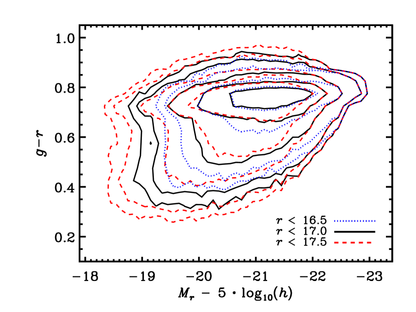
Figure 9.— The rest–frame $g-r$ color and $r$–band absolute magnitude distributions for magnitude–limited samples drawn from Gallazzi et al. (2005).

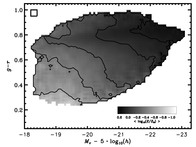
Figure 10.— The mean stellar metallicity, $Z$, as a function of rest–frame $g-r$ color and $r$–band absolute magnitude for galaxies brighter than $r=17.5$ in the catalog of Gallazzi et al. (2005). The mean metallicity is computed in a sliding box of width $\Delta M_{r}=0.2$ and height $\Delta(g-r)=0.05$, as shown in the upper left corner.

For these three magnitude–limited samples, we find a significant correlation between stellar metallicity and environment such that galaxies with more metal–rich stellar populations typically reside in more overdense environs, with the trend relatively independent of the magnitude limit of the sample (see Figure 11). This general correlation persists when focusing on just those galaxies that reside on the blue cloud (following Equation 1); however, the trend is considerably weaker.

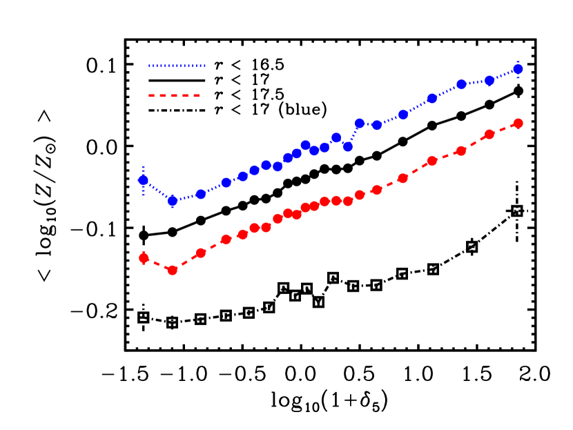
Figure 11.— The mean stellar metallicity, $<Z>$, as a function of local galaxy overdensity, $\log_{10}(1+\delta_{5})$, in magnitude–limited samples drawn from Gallazzi et al. (2005).

As stated in §4.4, for the main observational results of this paper to be connected to a particular physical property, that property must have a relationship with environment separate from that observed between color and luminosity (or stellar mass and star–formation rate). To test whether stellar metallicity has such a relationship with environment, we remove the dependence of environment on $g-r$ rest–frame color and $r$–band luminosity for a magnitude–limited $(r<17)$ sample of galaxies on the blue cloud, using the methodology detailed by Cooper et al. (2008a). In short, we subtract the mean overdensity at the color and luminosity of each galaxy from the measured overdensity:

$$\Delta_{5}=\log_{10}(1+\delta_{5})-<\log_{10}(1+\delta_{5})[g-r,M_{r}]>,$$ (1)

where the distribution of mean environment with color and absolute $r$–band magitude, $<\log_{10}(1+\delta_{5})[g-r,M_{r}]>$, is median smoothed on $\Delta(g-r)=0.15$ and $\Delta M_{r}=0.6$ scales prior to subtraction. This difference gives the “residual” environment, $\Delta_{5}$, which quantifies the overdensity about a galaxy relative to galaxies of like color and luminosity. As shown in Cooper et al. (2008a), this new measurement of environment shows no correlation with color and luminosity (by design) or stellar mass and star–formation rate.

We then study the relationship between residual environment and stellar metallicity, for our sample of star–forming galaxies with $r<17$. As shown in Figure 12, we find no significant residual trend between stellar metallicity and environment. That is, the mean residual environment is independent of stellar metallicity over the full range of metallicities probed. Thus, like morphology and surface brightness, stellar metallicity does not have a relationship with environment separate from that observed with color and luminosity.

Figure 12.— The dependence of mean residual environment, $\Delta_{5}$, on stellar metallicity for the blue galaxies in a magnitude–limited $(r<17)$ sample drawn from Gallazzi et al. (2005). The residual environment is computed following the methods of Cooper et al. (2008a). We find no relationship between stellar metallicity and environment beyond that observed between color, luminosity, and environment.

For the same sample of blue galaxies (with $r<17$), we also examine the correlation between luminosity–weighted mean stellar age and environment. Again, we use the age measurements of Gallazzi et al. (2005), which are based on model fits to the spectra features in the SDSS spectra. The model spectra utilized by Gallazzi et al. (2005) are derived from the population synthesis models of Bruzual & Charlot (2003) and span a broad range of star–formation histories. The models are simultaneously fit to a minimum set of metal– and age–sensitivie spectral indices (D4000, H$\beta$, H$\delta_{A}$ + H$\gamma_{A}$, [Mg₂Fe], and [MgFe]^′), yielding measurements of age and metallicity with typcial uncertainties on the order of $\sigma_{t}\lesssim 0.15$ dex and $\sigma_{Z}\lesssim 0.3$.

As shown in Figure 13, we find that there is a significant correlation between stellar age and absolute local environment along the blue cloud; galaxies with older stellar populations tend to reside in overdense environs relative to their counterparts with younger stellar composition. This effect is far from surprising given the correlation between stellar age and mass, where more massive systems tend to have more enriched and older stellar populations (see Fig. 8 of Gallazzi et al., 2005).

Figure 13.— The dependence of mean absolute environment, $log_{10}(1+\delta_{5})$, on stellar age, $(t)$, for the blue galaxies in a magnitude–limited $(r<17)$ sample drawn from Gallazzi et al. (2005). We find a significant relationship between mean stell age and environment such that older (i.e., more massive) galaxies favor overdense regions.

Now, we remove the mean dependence of environment on luminosity and color, again following Equation 1, and study the correlation between residual environment, $\Delta_{5}$, and stellar age. We find that there is no sigificant relationship between age and residual environment (see Figure 14). That is, stellar age — like stellar metallicity — does not have a relationship with environment separate from that observed with color and luminosity.

Figure 14.— The dependence of mean residual environment, $\Delta_{5}$, on stellar age for the blue galaxies in a magnitude–limited $(r<17)$ sample drawn from Gallazzi et al. (2005). The residual environment is computed following the methods of Cooper et al. (2008a). We find no relationship between stellar age and environment beyond that observed between color, luminosity, and environment.

References

- Abazajian et al. (2004) Abazajian, K. et al. 2004, AJ, 128, 502
- Adelman-McCarthy et al. (2008) Adelman-McCarthy, J. K. et al. 2008, ApJS, 175, 297
- Arnett (1982) Arnett, W. D. 1982, ApJ, 253, 785
- Astier et al. (2006) Astier, P. et al. 2006, A&A, 447, 31
- Balogh et al. (1998) Balogh, M. L., Schade, D., Morris, S. L., Yee, H. K. C., Carlberg, R. G., & Ellingson, E. 1998, ApJ, 504, L75+
- Bate (2005) Bate, M. R. 2005, MNRAS, 363, 363
- Bell et al. (2004) Bell, E. F. et al. 2004, ApJ, 608, 752
- Blanton et al. (2005a) Blanton, M. R., Eisenstein, D., Hogg, D. W., Schlegel, D. J., & Brinkmann, J. 2005a, ApJ, 629, 143
- Blanton & Roweis (2007) Blanton, M. R. & Roweis, S. 2007, AJ, 133, 734
- Blanton et al. (2003a) Blanton, M. R. et al. 2003a, AJ, 125, 2348
- Blanton et al. (2003b) —. 2003b, ApJ, 594, 186
- Blanton et al. (2005b) —. 2005b, AJ, 129, 2562
- Brinchmann et al. (2004) Brinchmann, J., Charlot, S., White, S. D. M., Tremonti, C., Kauffmann, G., Heckman, T., & Brinkmann, J. 2004, MNRAS, 351, 1151
- Bruzual & Charlot (2003) Bruzual, G. & Charlot, S. 2003, MNRAS, 344, 1000
- Calura et al. (2007) Calura, F., Matteucci, F., & Tozzi, P. 2007, MNRAS, 378, L11
- Cappellaro et al. (1999) Cappellaro, E., Evans, R., & Turatto, M. 1999, A&A, 351, 459
- Carlberg et al. (2008) Carlberg, R. G. et al. 2008, ApJ, 682, L25
- Carney et al. (2005) Carney, B. W., Aguilar, L. A., Latham, D. W., & Laird, J. B. 2005, AJ, 129, 1886
- Chabrier (2003) Chabrier, G. 2003, PASP, 115, 763
- Chandrasekhar (1931) Chandrasekhar, S. 1931, ApJ, 74, 81
- Charlot et al. (2002) Charlot, S., Kauffmann, G., Longhetti, M., Tresse, L., White, S. D. M., Maddox, S. J., & Fall, S. M. 2002, MNRAS, 330, 876
- Cole (1991) Cole, S. 1991, ApJ, 367, 45
- Cooper et al. (2005) Cooper, M. C., Newman, J. A., Madgwick, D. S., Gerke, B. F., Yan, R., & Davis, M. 2005, ApJ, 634, 833
- Cooper et al. (2008a) Cooper, M. C., Tremonti, C. A., Newman, J. A., & Zabludoff, A. I. 2008a, MNRAS, 1037
- Cooper et al. (2006) Cooper, M. C. et al. 2006, MNRAS, 370, 198
- Cooper et al. (2007) —. 2007, MNRAS, 376, 1445
- Cooper et al. (2008b) —. 2008b, MNRAS, 383, 1058
- Davé (2008) Davé, R. 2008, MNRAS, 385, 147
- Davé et al. (2006) Davé, R., Finlator, K., & Oppenheimer, B. D. 2006, MNRAS, 370, 273
- Davis & Geller (1976) Davis, M. & Geller, M. J. 1976, ApJ, 208, 13
- Dekel & Silk (1986) Dekel, A. & Silk, J. 1986, ApJ, 303, 39
- della Valle & Livio (1994) della Valle, M. & Livio, M. 1994, ApJ, 423, L31
- Djorgovski & Davis (1987) Djorgovski, S. & Davis, M. 1987, ApJ, 313, 59
- Domínguez et al. (2001) Domínguez, I., Höflich, P., & Straniero, O. 2001, ApJ, 557, 279
- Dressler (1980) Dressler, A. 1980, ApJ, 236, 351
- Dressler et al. (1997) Dressler, A. et al. 1997, ApJ, 490, 577
- Elbaz et al. (2007) Elbaz, D. et al. 2007, A&A, 468, 33
- Elmegreen (1999) Elmegreen, B. G. 1999, ApJ, 515, 323
- Faber & Jackson (1976) Faber, S. M. & Jackson, R. E. 1976, ApJ, 204, 668
- Finlator & Davé (2008) Finlator, K. & Davé, R. 2008, MNRAS, 385, 2181
- Frieman et al. (2008) Frieman, J. A. et al. 2008, AJ, 135, 338
- Gómez et al. (2003) Gómez, P. L. et al. 2003, ApJ, 584, 210
- Gal-Yam et al. (2003) Gal-Yam, A., Maoz, D., Guhathakurta, P., & Filippenko, A. V. 2003, AJ, 125, 1087
- Gallagher et al. (2005) Gallagher, J. S., Garnavich, P. M., Berlind, P., Challis, P., Jha, S., & Kirshner, R. P. 2005, ApJ, 634, 210
- Gallagher et al. (2008) Gallagher, J. S., Garnavich, P. M., Caldwell, N., Kirshner, R. P., Jha, S. W., Li, W., Ganeshalingam, M., & Filippenko, A. V. 2008, ApJ, 685, 752
- Gallazzi et al. (2005) Gallazzi, A., Charlot, S., Brinchmann, J., White, S. D. M., & Tremonti, C. A. 2005, MNRAS, 362, 41
- Gerke et al. (2005) Gerke, B. F. et al. 2005, ApJ, 625, 6
- Graham et al. (2008) Graham, M. L. et al. 2008, AJ, 135, 1343
- Greggio (2005) Greggio, L. 2005, A&A, 441, 1055
- Greggio et al. (2008) Greggio, L., Renzini, A., & Daddi, E. 2008, MNRAS, 388, 829
- Hachisu et al. (1996) Hachisu, I., Kato, M., & Nomoto, K. 1996, ApJ, 470, L97+
- Hamuy et al. (1995) Hamuy, M., Phillips, M. M., Maza, J., Suntzeff, N. B., Schommer, R. A., & Aviles, R. 1995, AJ, 109, 1
- Hamuy et al. (1996) Hamuy, M., Phillips, M. M., Suntzeff, N. B., Schommer, R. A., Maza, J., & Aviles, R. 1996, AJ, 112, 2391
- Hamuy et al. (2000) Hamuy, M., Trager, S. C., Pinto, P. A., Phillips, M. M., Schommer, R. A., Ivanov, V., & Suntzeff, N. B. 2000, AJ, 120, 1479
- Han & Podsiadlowski (2004) Han, Z. & Podsiadlowski, P. 2004, MNRAS, 350, 1301
- Hogg et al. (2004) Hogg, D. W., Blanton, M. R., Brinchmann, J., Eisenstein, D. J., Schlegel, D. J., Gunn, J. E., McKay, T. A., Rix, H., Bahcall, N. A., Brinkmann, J., & Meiksin, A. 2004, ApJ, 601, L29
- Howell et al. (2008) Howell, D. A. et al. 2008, ArXiv e-prints
- Iben & Tutukov (1984) Iben, Jr., I. & Tutukov, A. V. 1984, ApJS, 54, 335
- Ivanov et al. (2000) Ivanov, V. D., Hamuy, M., & Pinto, P. A. 2000, ApJ, 542, 588
- Kaiser (1987) Kaiser, N. 1987, MNRAS, 227, 1
- Kasen & Plewa (2005) Kasen, D. & Plewa, T. 2005, ApJ, 622, L41
- Kasen et al. (2009) Kasen, D., Röpke, F. K., & Woosley, S. E. 2009, Nature, 460, 869
- Kasen & Woosley (2007) Kasen, D. & Woosley, S. E. 2007, ApJ, 656, 661
- Kauffmann et al. (2003) Kauffmann, G. et al. 2003, MNRAS, 341, 33
- Kennicutt (1998) Kennicutt, Jr., R. C. 1998, ApJ, 498, 541
- Kobayashi et al. (2000) Kobayashi, C., Tsujimoto, T., & Nomoto, K. 2000, ApJ, 539, 26
- Kobayashi et al. (1998) Kobayashi, C., Tsujimoto, T., Nomoto, K., Hachisu, I., & Kato, M. 1998, ApJ, 503, L155+
- Kroupa (2007) Kroupa, P. 2007, ArXiv Astrophysics e-prints
- Lupton et al. (1999) Lupton, R. H., Gunn, J. E., & Szalay, A. S. 1999, AJ, 118, 1406
- Machida (2008) Machida, M. N. 2008, ApJ, 682, L1
- Machida et al. (2009) Machida, M. N., Omukai, K., Matsumoto, T., & Inutsuka, S.-i. 2009, ArXiv e-prints
- Mann & Whitney (1947) Mann, H. B. & Whitney, D. R. 1947, The Annals of Mathematical Statistics, 18, 50
- Mannucci et al. (2006) Mannucci, F., Della Valle, M., & Panagia, N. 2006, MNRAS, 370, 773
- Mannucci et al. (2005) Mannucci, F., Della Valle, M., Panagia, N., Cappellaro, E., Cresci, G., Maiolino, R., Petrosian, A., & Turatto, M. 2005, A&A, 433, 807
- Mannucci et al. (2008) Mannucci, F., Maoz, D., Sharon, K., Botticella, M. T., Della Valle, M., Gal-Yam, A., & Panagia, N. 2008, MNRAS, 383, 1121
- Maoz (2008) Maoz, D. 2008, MNRAS, 384, 267
- Maoz et al. (2005) Maoz, D., Waxman, E., & Loeb, A. 2005, ApJ, 632, 847
- Matteucci et al. (2006) Matteucci, F., Panagia, N., Pipino, A., Mannucci, F., Recchi, S., & Della Valle, M. 2006, MNRAS, 372, 265
- Matteucci & Vettolani (1988) Matteucci, F. & Vettolani, G. 1988, A&A, 202, 21
- Moustakas et al. (2006) Moustakas, J., Kennicutt, Jr., R. C., & Tremonti, C. A. 2006, ApJ, 642, 775
- Oemler & Tinsley (1979) Oemler, Jr., A. & Tinsley, B. M. 1979, AJ, 84, 985
- Oke & Gunn (1983) Oke, J. B. & Gunn, J. E. 1983, ApJ, 266, 713
- Perlmutter et al. (1999) Perlmutter, S. et al. 1999, ApJ, 517, 565
- Pinto & Eastman (2000) Pinto, P. A. & Eastman, R. G. 2000, ApJ, 530, 744
- Postman & Geller (1984) Postman, M. & Geller, M. J. 1984, ApJ, 281, 95
- Press et al. (1992) Press, W. H., Teukolsky, S. A., Vetterling, W. T., & Flannery, B. P. 1992, Numerical recipes in C. The art of scientific computing (Cambridge: University Press, —c1992, 2nd ed.)
- Prieto et al. (2008) Prieto, J. L., Stanek, K. Z., & Beacom, J. F. 2008, ApJ, 673, 999
- Pritchet et al. (2008) Pritchet, C. J., Howell, D. A., & Sullivan, M. 2008, ApJ, 683, L25
- Riess et al. (1998) Riess, A. G. et al. 1998, AJ, 116, 1009
- Sako et al. (2008) Sako, M. et al. 2008, AJ, 135, 348
- Sato et al. (2007) Sato, K., Tokoi, K., Matsushita, K., Ishisaki, Y., Yamasaki, N. Y., Ishida, M., & Ohashi, T. 2007, ApJ, 667, L41
- Scannapieco et al. (2008) Scannapieco, C., Tissera, P. B., White, S. D. M., & Springel, V. 2008, MNRAS, 389, 1137
- Scannapieco & Bildsten (2005) Scannapieco, E. & Bildsten, L. 2005, ApJ, 629, L85
- Schaye et al. (2003) Schaye, J., Aguirre, A., Kim, T.-S., Theuns, T., Rauch, M., & Sargent, W. L. W. 2003, ApJ, 596, 768
- Selman & Melnick (2008) Selman, F. J. & Melnick, J. 2008, ApJ, 689, 816
- Sharon et al. (2007) Sharon, K., Gal-Yam, A., Maoz, D., Filippenko, A. V., & Guhathakurta, P. 2007, ApJ, 660, 1165
- Shen et al. (2003) Shen, S., Mo, H. J., White, S. D. M., Blanton, M. R., Kauffmann, G., Voges, W., Brinkmann, J., & Csabai, I. 2003, MNRAS, 343, 978
- Sivanandam et al. (2008) Sivanandam, S., Zabludoff, A. I., Zaritsky, D., Gonzalez, A. H., & Kelson, D. D. 2008, ArXiv e-prints
- Smith et al. (2005) Smith, G. P., Treu, T., Ellis, R. S., Moran, S. M., & Dressler, A. 2005, ApJ, 620, 78
- Strateva et al. (2001) Strateva, I. et al. 2001, AJ, 122, 1861
- Strolger et al. (2002) Strolger, L.-G. et al. 2002, AJ, 124, 2905
- Sullivan et al. (2006a) Sullivan, M. et al. 2006a, AJ, 131, 960
- Sullivan et al. (2006b) —. 2006b, ApJ, 648, 868
- Timmes et al. (2003) Timmes, F. X., Brown, E. F., & Truran, J. W. 2003, ApJ, 590, L83
- Tornambe & Matteucci (1986) Tornambe, A. & Matteucci, F. 1986, MNRAS, 223, 69
- Tout (2005) Tout, C. A. 2005, in Astronomical Society of the Pacific Conference Series, Vol. 330, The Astrophysics of Cataclysmic Variables and Related Objects, ed. J.-M. Hameury & J.-P. Lasota, 279–+
- Townsley et al. (2009) Townsley, D. M., Jackson, A. P., Calder, A. C., Chamulak, D. A., Brown, E. F., & Timmes, F. X. 2009, ArXiv e-prints
- Tremonti et al. (2004) Tremonti, C. A. et al. 2004, ApJ, 613, 898
- Umeda et al. (1999a) Umeda, H., Nomoto, K., Kobayashi, C., Hachisu, I., & Kato, M. 1999a, ApJ, 522, L43
- Umeda et al. (1999b) Umeda, H., Nomoto, K., Yamaoka, H., & Wanajo, S. 1999b, ApJ, 513, 861
- van den Bergh (1990) van den Bergh, S. 1990, PASP, 102, 1318
- van Dokkum (2008) van Dokkum, P. G. 2008, ApJ, 674, 29
- Wall & Jenkins (2003) Wall, J. V. & Jenkins, C. R. 2003, Practical Statistics for Astronomers (Princeton Series in Astrophysics)
- Webbink (1984) Webbink, R. F. 1984, ApJ, 277, 355
- Whelan & Iben (1973) Whelan, J. & Iben, I. J. 1973, ApJ, 186, 1007
- Willmer et al. (2006) Willmer, C. N. A. et al. 2006, ApJ, 647, 853
- Woosley & Weaver (1995) Woosley, S. E. & Weaver, T. A. 1995, ApJS, 101, 181
- Yan et al. (2006) Yan, R., Newman, J. A., Faber, S. M., Konidaris, N., Koo, D., & Davis, M. 2006, ApJ, 648, 281
- Yasui et al. (2008) Yasui, C., Kobayashi, N., Tokunaga, A. T., Saito, M., & Tokoku, C. 2008, in Astronomical Society of the Pacific Conference Series, Vol. 396, Astronomical Society of the Pacific Conference Series, ed. J. G. Funes & E. M. Corsini, 225–+
- Yasui et al. (2006) Yasui, C., Kobayashi, N., Tokunaga, A. T., Terada, H., & Saito, M. 2006, ApJ, 649, 753
- York et al. (2000) York, D. G. et al. 2000, AJ, 120, 1579
- Yungelson & Livio (2000) Yungelson, L. R. & Livio, M. 2000, ApJ, 528, 108
- Zehavi et al. (2005) Zehavi, I. et al. 2005, ApJ, 630, 1