Vast multiplicity of very singular self-similar solutions of a semilinear higher-order diffusion equation with time-dependent absorption

Abstract.

As a basic model, the Cauchy problem in ${\mathbb{R}}^{N}\times{\mathbb{R}}_{+}$ for the $2m$th-order semilinear parabolic equation of the diffusion-absorption type

$$u_{t}=-(-\Delta)^{m}u-t^{\alpha}|u|^{p-1}u,\quad\mbox{with}\,\,p>1,\,\,\alpha>0,\,\,\,m\geq 2,$$

with singular initial data $u_{0}\not=0$ such that $u_{0}(x)=0$ for any $x\not=0$ is studied. The additional multiplier $h(t)=t^{\alpha}\to 0$ as $t\to 0$ in the absorption term plays a role of time-dependent non-homogeneous potential that affects the strength of the absorption term in the PDE. Existence and nonexistence of the corresponding very singular solutions (VSSs) is studied. For $m=1$ and $h(t)\equiv 1$, first nonexistence result for $p\geq p_{0}=1+\frac{2}{N}$ was proved in the celebrated paper by Brezis and Friedman in 1983. Existence of VSSs in the complement interval $1<p<p_{0}$ was established in the middle of the 1980s.

The main goal is to justify that, in the subcritical range $1<p<p_{0}=1+\frac{2m(1+\alpha)}{N}$, there exists a finite number of different VSSs of the self-similar form

$$u_{*}(x,t)=t^{-\beta}V(y),\quad y=x/t^{\frac{1}{2m}},\quad\beta=\frac{1+\alpha}{p-1},$$

where each $V$ is an exponentially decaying as $y\to\infty$ solution of the elliptic equation

$$-(-\Delta)^{m}V+\mbox{$\frac{1}{2m}$}\,y\cdot\nabla V+\beta V-|V|^{p-1}V=0\quad\mbox{in}\quad{\mathbb{R}}^{N}.$$

Complicated families of VSSs in 1D and also non-radial VSS patterns in ${\mathbb{R}}^{N}$ are detected. Some of these VSS profiles $V_{l}$ are shown to bifurcate from $0$ at the bifurcation exponents

$$p_{l}=1+\frac{2m(1+\alpha)}{l+N},\quad\mbox{where}\,\,\,l=0,1,2,...\,.$$

1. Introduction: VSSs for higher-order diffusion-absorption PDEs

1.1. Diffusion-absorption model

Our basic model is the $2m$th-order semilinear heat equation in ${\mathbb{R}}^{N}\times{\mathbb{R}}_{+}$ with non-autonomous (non-homogeneous) absorption term

(1.1) $$u_{t}=-(-\Delta)^{m}u-h(t)|u|^{p-1}u\quad(p>1,\,\,\,m\geq 2),$$

where the given function $h(t)$ satisfies

$$h(t)>0,\quad h(t)\to 0\quad\mbox{as \,$t\to 0$}.$$

For $m=1$ and $h=1$, the critical Fujita-like exponent $p_{0}=1+\frac{2}{N}$ and existence-nonexistence of very singular solutions (VSSs) was derived since the 1980s; see first principal results of the 1980s in [4, 15, 5, 12, 21, 22, 23], and a long list of references in [18, Ch. 4]. In the higher-order case $m\geq 2$ and $h=1$, such an investigation has been performed in [14, 17, 19]. The influence to VSSs of non-homogeneous potentials $h(t)$ was first studied in Marcus–Véron [26] in the case $m=1$; see more recent extensions in [31].

1.2. Similarity VSSs: towards a non-variational problem

The layout of the paper is as follows. We investigate the phenomena associated with the non-homogeneous term and consider the power case

(1.2) $$h(t)=t^{\alpha},\quad\mbox{with the fixed exponent}\,\,\,\alpha>-1\quad\big{(}\mbox{so that}\quad\int_{0}h(t)\,{\mathrm{d}}t<\infty\big{)}.$$

In Section 2, for the higher-order equation (1.1) with $m\geq 2$, we study the existence and multiplicity of similarity solutions and show that, in the subcritical range $p\in(1,p_{0})$, with the critical (Fujita-like) exponent

$$p_{0}=1+\frac{2m(1+\alpha)}{N},$$

there exist VSSs of the similarity form

(1.3) $$u_{*}(x,t)=t^{-\beta}V(y),\quad y=x/t^{\frac{1}{2m}},\quad\mbox{with}\,\,\,\beta=\frac{1+\alpha}{p-1}>0,$$

where $V$ is a non-trivial radial solution of the elliptic equation

(1.4) $$\left\{\begin{matrix}{\bf B}_{1}V-|V|^{p-1}V\equiv-(-\Delta)^{m}V+\mbox{$\frac{1}{2m}$}\,y\cdot\nabla V+\beta V-|V|^{p-1}V=0\quad\mbox{in}\quad{\mathbb{R}}^{N},\vskip 3.0pt plus 1.0pt minus 1.0pt\vskip 3.0pt plus 1.0pt minus 1.0pt\\ V(y)\,\,\,\mbox{decays exponentially fast as}\,\,\,|y|\to\infty.\qquad\qquad\qquad\qquad\qquad\qquad\quad\end{matrix}\right.$$

Passing to the limit $t\to 0^{+}$ in (1.3) yields the initial function satisfying

(1.5) $$u(x,0)=0\quad\mbox{for all}\,\,\,x\not=0,$$

which nevertheless is not a finite measure, and this reinforces the notion of very singular solutions for (1.3). Condition in (1.4) on exponential decay at infinity is naturally enforced by introducing weighted $L^{2}$ and Sobolev spaces; details are given in in Section 2.

1.3. On main results

The main goal is to detect the whole range of VSS profiles by using spectral properties of the linear operator ${\bf B}_{1}$ in (1.4) and bifurcation theory. This determines a countable number of $p$-bifurcation branches of VSS profiles in the subcritical range $p<p_{0}$ that, for any $\alpha>-1$, are originated at the bifurcation points

(1.6) $$p_{l}=1+\frac{2m(1+\alpha)}{N+l},\quad l=0,1,2,...\,.$$

This also yields $\alpha$-bifurcation points,

(1.7) $$\alpha_{l}=\frac{(p-1)(N+l)}{2m}-1,\quad l=0,1,2,...\,.$$

In Section 3, using numerical experiments, we show that, surprisingly, the whole picture of branches of VSS similarity profiles is essentially more complicated than that for $\alpha=0$ studied in [19]. It turns out that even in 1D for sufficiently large $\alpha>0$, the whole set of VSS profiles consists of various families of solutions of different geometric shapes. In addition, this includes new branches that are expected to appear at saddle-node (turning) bifurcation points in $\alpha$. In Section 4, for future use for non-power potentials such as

(1.8) $$h_{*}(t)={\mathrm{e}}^{-1/t}\,,$$

we are particularly interested in the study of the limit behaviour of such VSSs as $\alpha\to+\infty$. Some nonexistence results of VSSs in the range $p\geq p_{0}$ are proved in Section 5.

It is necessary to mention that for, any $m\geq 2$, the problem (1.4) even in 1D is not variational (it is for $m=1$ only), so the operators there are not potential in any topology. Moreover, even the linear principal part ${\bf B}_{1}$ therein in not self-adjoint (symmetric) in any weighted space $L^{2}_{\rho}$. In addition, the corresponding parabolic flow is not order-preserving in view of the lack of the Maximum Principle (again applies for $m=1$ only).

Therefore, for describing the complicated discrete sets $\{V_{\sigma_{k}}\}$, where $\sigma_{k}$ is a multiindex (see Section 3), we are going to use a machinery of various bifurcation-branching methods of nonlinear analysis. Nevertheless, many of our final conclusions on the global behaviour of bifurcation diagrams of $V$’s remain formal, and we do not expect that a reasonably simple justification can be achieved soon. Therefore, we heavily rely on numerical construction of, at least, am couple of hundreds of similarity profiles. These numerics are also not that easy at all. Often, the reliable numerics will be the only tool to detect this vast multiplicity of VSS profiles of (1.4) far away from bifurcation points.

2. VSSs profiles: local bifurcation theory

Thus, consider the Cauchy problems for the PDE (1.1) with the power potential (1.1).

2.1. The fundamental solution of the poly-harmonic equation

This is

(2.1) $$b(x,t)=t^{-\frac{N}{2m}}F(y),\quad y=x/t^{\frac{1}{2m}},$$

being the fundamental solution of the linear poly-harmonic equation

(2.2) $$u_{t}=-(-\Delta)^{m}u.$$

The rescaled kernel $F$ is then the unique radial solution of the elliptic equation

(2.3) $${\bf B}F\equiv-(-\Delta)^{m}F+{\mathcal{L}}_{0}F=0\,\,\,\mbox{in}\,\,{\mathbb{R}}^{N},\,\,\,\int F=1;\quad{\mathcal{L}}_{0}=\mbox{$\frac{1}{2m}$}\,y\cdot\nabla+\mbox{$\frac{N}{2m}$}\,I,$$

satisfying for some positive constants $D>1$ and $d>0$ depending on $m$ and $N$ [10]

(2.4) $$|F(y)|<D\bar{F}(y)\equiv D\omega_{1}{\mathrm{e}}^{-d|y|^{\alpha}}\,\,{\rm in}\,\,{\mathbb{R}}^{N},\quad\alpha=\mbox{$\frac{2m}{2m-1}$}\in(1,2),$$

$\omega_{1}>0$ being a normalization constant such that $\int\bar{F}=1$.

It turns out that the linear operator ${\bf B}_{1}$ in equation (1.4) is connected with the operator (2.3) for the rescaled kernel $F$ as follows:

(2.5) $${\bf B}_{1}={\bf B}+c_{1}I,\quad\mbox{where}\,\,\,c_{1}=\mbox{$\frac{N(p_{0}-p)}{2m(p-1)}$}.$$

2.2. The point spectrum of the non self-adjoint operator ${\bf B}$

We consider the linear operator ${\bf B}$ given in (2.3) in the weighted space $L^{2}_{\rho}({\bf R}^{N})$ with the exponentially growing weight function

(2.6) $$\rho(y)={\mathrm{e}}^{a|y|^{\alpha}}>0\quad{\rm in}\,\,\,{\mathbb{R}}^{N},$$

where $a\in(0,2d)$ is a sufficiently small constant. We ascribe to ${\bf B}$ the domain $H^{2m}_{\rho}({\bf R}^{N})$ being a Hilbert space with the norm

$$\|v\|^{2}=\int\rho(y)\mbox{$\sum_{k=0}^{2m}$}\,|D^{k}v(y)|^{2}\,{\mathrm{d}}y,$$

induced by the corresponding inner product. We have $H^{2m}_{\rho}\subset L^{2}_{\rho}\subset L^{2}$. The spectral properties ${\bf B}$ are as follows [9]:

Lemma 2.1.

(i) ${\mathbf{B}}:H^{2m}_{\rho}\to L^{2}_{\rho}$ is a bounded linear operator with the real point spectrum

(2.7) $$\sigma({\mathbf{B}})=\big{\{}\lambda_{l}=-\mbox{$\frac{l}{2m}$},\,\,l=0,1,2,...\big{\}}.$$

The eigenvalues $\lambda_{l}$ have finite multiplicity with eigenfunctions

(2.8) $$\psi_{\beta}(y)=\frac{(-1)^{|\beta|}}{\sqrt{\beta!}}\,D^{\beta}F(y),\quad\mbox{with any}\,\,\,|\beta|=l\geq 0.$$

(ii) The set of eigenfunctions $\Phi=\{\psi_{\beta},\,|\beta|=0,1,2,...\}$ is complete and closed in $L^{2}_{\rho}$.

In the classical second-order case $m=1$, we have that

$$F(y)=(4\pi)^{-\frac{N}{2}}{\mathrm{e}}^{-\frac{1}{4}\,{|y|^{2}}}$$

is the rescaled positive Gaussian kernel and the eigenfunctions are

$$\psi_{\beta}(y)={\mathrm{e}}^{-\frac{1}{4}\,|y|^{2}}H_{\beta}(y),$$

where $H_{\beta}$ are separable Hermite polynomials in ${\bf R}^{N}$ [3, p. 48]. The operator ${\bf B}$, with the domain $H_{\rho}^{2}$ and the weight $\rho={\mathrm{e}}^{|y|^{2}/4}$, is self-adjoint and the eigenfunctions form an orthogonal basis in $L^{2}_{\rho}$.

Lemma 2.1 gives the centre and stable subspaces of ${\bf B}$, $E^{c}={\rm Span}\{\psi_{0}=F\}$, $E^{s}={\rm Span}\{\psi_{\beta},\,|\beta|>0\}$.

2.3. The polynomial eigenfunctions of the adjoint operator ${\bf B}^{*}$

Consider the adjoint operator to ${\bf B}$,

(2.9) $${\bf B}^{*}=-(-\Delta)^{m}-\mbox{$\frac{1}{2m}$}\,y\cdot\nabla\,.$$

For $m=1$, the following representation holds:

$${\bf B}^{*}\equiv\frac{1}{\rho^{*}}\,\nabla\cdot(\rho^{*}\nabla),\,\,\,\mbox{with}\,\,\,{\mathcal{D}}({\bf B}^{*})=H^{2}_{\rho^{*}},\quad\mbox{where}\quad\rho^{*}(y)={\mathrm{e}}^{-\frac{1}{4}\,|y|^{2}},$$

is self-adjoint in $L^{2}_{\rho^{*}}$ and has a discrete spectrum. The eigenfunctions form an orthonormal basis in $L^{2}_{\rho^{*}}$ and the classical Hilbert-Schmidt theory applies [3].

For $m>1$, we consider ${\bf B}^{*}$ in $L^{2}_{\rho^{*}}$ with the exponentially decaying weight function

$$\rho^{*}(y)=\frac{1}{\rho(y)}\equiv{\mathrm{e}}^{-a|y|^{\alpha}}>0.$$

Lemma 2.2.

(i) ${\bf B}^{*}:H^{2m}_{\rho^{*}}\to L^{2}_{\rho^{*}}$ is a bounded linear operator with the same spectrum as ${\bf B}$, $(\ref{spec1})$. The eigenfunctions $\psi_{\beta}^{*}(y)$ with $|\beta|=l$ are $l$th-order polynomials

(2.10) $$\psi_{\beta}^{*}(y)=\frac{1}{\sqrt{\beta!}}\big{[}y^{\beta}+\mbox{$\sum_{j=1}^{\lfloor\frac{|\beta|}{2m}\rfloor}\frac{1}{j!}$}(-\Delta)^{mj}y^{\beta}\big{]}.$$

(ii) The set $\{\psi_{\beta}^{*}\}$ is complete in $L^{2}_{\rho^{*}}$.

From this definition of the adjoint eigenfunctions, the orthonormality condition holds

(2.11) $$\langle\psi_{\beta},\psi_{\gamma}^{*}\rangle=\delta_{\beta\gamma},$$

where $\langle\cdot,\cdot\rangle$ denotes the standard $L^{2}$ inner product. For $m=1$, both (2.7) and (2.10) are well-known properties of the separable Hermite polynomials, [3].

2.4. Bifurcations at $p=p_{l}$: local existence of the VSSs

It follows from (2.5) and the above lemmas that the only possible bifurcation points of VSSs are obtained from

(2.12) $$c_{1}=-\lambda_{l}\quad\Longrightarrow\quad p=p_{l}=1+\frac{2m(1+\alpha)}{N+l},\,\,\ l=0,1,2,...\,.$$

We justify these bifurcation phenomena. Taking $p$ near the critical values as defined in (2.12), we look for small solutions of the problem (1.4). At $p=p_{l}$, the linear operator ${\bf B}_{1}$ has a nontrivial kernel, hence, the following result:

Proposition 2.1.

Let for an integer $l\geq 0$, the eigenvalue $\lambda_{l}=-\frac{l}{2m}$ of operator $(\ref{ODEf})$ be of odd multiplicity. Then the exponent in $(\ref{pcrit})$ is a bifurcation point for $(\ref{1.7R})$.

Proof. This result is standard in bifurcation theory; see [8, p. 381] and similar results in a related problem in [19, § 6]. Necessary spectral properties of the linearized operator are given in [9]. We present some comments concerning the linearized operators involved.

Consider in $H^{2m}_{\rho}$ the equation

(2.13) $$\hat{{\bf B}}V=-(1+c_{1})V+|V|^{p-1}V,\quad\hat{{\bf B}}={\bf B}_{1}-(1+c_{1})I\equiv{\bf B}-I.$$

The spectrum of $\hat{{\bf B}}$ is a translation of that of ${\bf B}$, $\sigma(\hat{{\bf B}})=\{-1-\frac{l}{2m}\}$, and consists of strictly negative eigenvalues. The inverse operator $\hat{{\bf B}}^{-1}$ is known to be compact (Proposition 2.4 in [9]). Therefore, in the corresponding integral equation

(2.14) $$V={\bf A}(V)\equiv-(1+c_{1})\hat{{\bf B}}^{-1}V+\hat{{\bf B}}^{-1}|V|^{p-1}V,$$

the right-hand side contains a compact Hammerstein operator in $L^{q}_{\rho}({\mathbb{R}}^{N})$ space for some $q\geq 1$ [24, p. 38] (see details on the resolvent of ${\bf B}$ in [6]). In this application, there exist certain technical difficulties in checking compactness of this Hammerstein operators in weighted $L^{q}$-spaces over whole ${\mathbb{R}}^{N}$. As an alternative, we can use Ladyzhenskii’s theorem [24, p. 34] establishing compactness in $C$.

To avoid this technicalities, we use [8, Thm. 28.1] where no assumptions on compactness of the vector field are necessary. The main hypothesis therein is oriented to the linearized operator in (2.14) that is assumed to be Fredholm of index zero at bifurcation values (which is true by [9]). Then the result is first obtained for truncated uniformly bounded nonlinearity instead of $|V|^{p-1}V$ (see [19, p. 1088]), for which all the hypotheses are valid. Then bifurcations in the truncated problem (2.14) are always guaranteed if the derivative ${\bf A}^{\prime}(0)=-(1+c_{1})\hat{{\bf B}}^{-1}$ has the eigenvalue $1$ of odd multiplicity. (cf. also [24, p. 196] for compact integral operators).

Thus, bifurcations in the problem (2.14) occur if the derivative ${\bf A}^{\prime}(0)=-(1+c_{1})\hat{{\bf B}}^{-1}$ has the eigenvalue $1$ of odd multiplicity. Since $\sigma({\bf A}^{\prime}(0))=\{(1+c_{1})/(1+\frac{l}{2m})\},$ we arrive at critical values (2.12). By construction, the solutions of (2.14) for $p\approx p_{l}$ are small in $L^{2}_{\rho}$ and, as can be seen from the properties of the inverse operator, in $H^{2m}_{\rho}$. Since the weight $\rho(y)$ is a monotone growing function as $|y|\to\infty$, this implies that $V\in H^{2m}_{\rho}$ in the subcritical Sobolev range

(2.15) $$1<p<p_{S}=\frac{N+2m}{N-2m}$$

(which is true in our VSS range $p\leq p_{0}$) is a uniformly bounded, continuous function by standard elliptic regularity results and embedding theorems; these can be found in [27] and [32]. For $N<2m$, the result is straightforward in view of embedding [32, p. 5]

$$H^{m}({\mathbb{R}}^{N})\subset C({\mathbb{R}}^{N})\quad(N<2m).$$

Let us mention related boundedness results of parabolic orbits of (1.4) ($\alpha=0$) in the range (2.15) obtained in [19, § 2] by Henry’s version of Gronwall’s inequality with power kernel and scaling arguments.

Therefore, for $p\approx p_{l}$, we have bounded, uniformly small solutions of (2.14) only. By interior regularity results for elliptic equations, these solutions are smooth enough to be classical ones of the differential equation (2.13). ∎

Thus, $l=0$ is always a bifurcation point since $p_{0}=0$ is simple. In general, for $l=1,2,...$, the odd multiplicity occurs depending on the dimension $N$. In particular, for $l=1$, the multiplicity is $N$, and for $l=2$, it is $\frac{N(N+1)}{2}$. In the case of the even multiplicity of $\lambda_{l}$, an extra analysis is necessary to guarantee that a bifurcation occurs, [25]. It is important that, for key applications, namely, for $N=1$ and for the radial setting in ${\mathbb{R}}^{N}$, the eigenvalues (2.7) are simple and (2.12) are bifurcation points.

Since the nonlinear perturbation term in the integral equation (2.14) is an odd sufficiently smooth operator, we easily obtain the following result describing the local behaviour of bifurcation branches, see [24] and [25, Ch. 8].

Proposition 2.2.

Let $\lambda_{l}$ be a simple eigenvalue of ${\bf B}$ with eigenfunction $\psi_{l}$. Denoting

(2.16) $$\kappa_{l}=\langle|\psi_{l}|^{p-1}\psi_{l},\psi_{l}^{*}\rangle,$$

we have that problem $(\ref{1.7R})$ has (i) precisely two small solutions for $p\approx p_{l}^{-}$ and no solutions for $p\approx p_{l}^{+}$ if $\kappa_{l}>0$, and (ii) precisely two small solutions for $p\approx p_{l}^{+}$ and no solutions for $p\approx p_{l}^{-}$ if $\kappa_{l}<0$.

In order to describe the asymptotics of solutions as $p\to p_{l}$, we apply the Lyapunov-Schmidt method ([25, Ch. 8]) to equation (2.14) with the operator ${\bf A}$ being differentiable at $0$. Since under the assumptions of Proposition 2.2 the kernel $E_{0}={\rm ker\,}{\bf A}^{\prime}(0)={\rm Span\,}\{\psi_{l}\}$ is one-dimensional, denoting by $E_{1}$ the complementary (orthogonal to $\psi_{l}^{*}$) invariant subspace, we set $V=V_{0}+V_{1}$, where $V_{0}=\varepsilon_{l}\psi_{l}\in E_{0}$ and

$$V_{1}=\sum_{k\not=l}\varepsilon_{k}\psi_{k}\in E_{1}.$$

Let $P_{0}$ and $P_{1}$, $P_{0}+P_{1}=I$, be projections onto $E_{0}$ and $E_{1}$ respectively. Projecting (2.14) with $n=\infty$ onto $E_{0}$ yields

(2.17) $$\gamma_{l}\varepsilon_{l}=\langle\hat{\bf B}^{-1}(|V|^{p-1}V),\psi_{l}^{*}\rangle,\quad\gamma_{l}=1-\frac{1+c_{1}}{1+\frac{l}{2m}}=-\mbox{$\frac{(N+l)s}{(1+\alpha)(p-1)(2m+l)}$},$$

where $s=p_{l}-p$. By the general bifurcation theory (see e.g. [25, p. 355], [8, p. 383], and branching approaches in [33]; note that operator ${\bf A}^{\prime}(0)$ is Fredholm of index zero), the equation for $V_{1}$ can be solved and this gives $V_{1}=o(\varepsilon_{l})$ as $\varepsilon_{l}\to 0$, so that $\varepsilon_{l}$ is calculated from the Lyapunov bifurcation equation (2.17) as follows

$$\gamma_{l}\varepsilon_{l}=|\varepsilon_{l}|^{p-1}\varepsilon_{l}\langle\hat{\bf B}^{-1}|\psi_{l}|^{p-1}\psi_{l},\psi_{l}^{*}\rangle+o(|\varepsilon_{l}|^{p})\,\,\Longrightarrow\,\,|\varepsilon_{l}|^{p-1}=\hat{c}_{l}[(p_{l}-p)+o(1)],$$

where $\hat{c}_{l}=\mbox{$\frac{(N+l)^{2}}{4m^{2}(1+\alpha)\kappa_{l}}$}.$ Here, we have performed calculations as follows:

$$\langle\hat{\bf B}^{-1}\psi_{l}^{p},\psi_{l}^{*}\rangle=\langle\psi_{l}^{p},(\hat{\bf B}^{*})^{-1}\psi_{l}^{*}\rangle=-\kappa_{l}/(1+\mbox{$\frac{l}{2m}$}).$$

It is natural to require $\kappa_{l}>0$, though this is not always true for $\alpha>0$; see a closed curve of solutions in Figure 2 (for $\alpha=0$ the branches were detected to be always monotone, [19]). In view of the orthonormality property (2.11), for $p=1$ we have $\kappa_{l}=1$, so that by continuity we can guarantee that

(2.18) $$\kappa_{l}>0\quad\mbox{at least for all}\,\,\,p\approx 1^{+}.$$

Thus, we obtain a countable sequence of bifurcation points (2.12) satisfying $p_{l}\to 1^{+}$ as $l\to\infty$, with typical pitch-fork bifurcation branches appearing in a left-hand neighbourhood, for $p<p_{l}$. The behaviour of solutions in $H^{2m}_{\rho}$ and uniformly takes the form

(2.19) $$V_{l}(y)=\pm\left[\hat{c}_{l}(p_{l}-p)\right]^{1/(p-1)}(\psi_{l}(y)+o(1))\quad\mbox{as}\,\,\,p\to p_{l}^{-}.$$

We now prove the main result concerning “local” existence and stability of the VSS solution with the similarity profile $V_{0}(y)$ corresponding to the first bifurcation point, $p=p_{0}$. If $\kappa_{0}>0$, as expected, then two bifurcation branches exist for $p<p_{0}$.

Theorem 2.1.

For $p\approx p_{0}^{-}$, the problem $(\ref{1.7R})$ admits a solution $V_{0}(y)\not\equiv 0$ provided that $\frac{2m}{N}$ is small enough, and then it is an asymptotically stable stationary solution.

Proof. As we have shown, a continuous branch bifurcating at $p=p_{0}^{-}$ exists if

(2.20) $$\kappa_{0}=\langle|\psi_{0}|^{p_{0}-1}\psi_{0},\psi_{0}^{*}\rangle\equiv\int|F|^{\frac{2m}{N}}F\,>0\quad(\psi_{0}^{*}\equiv 1).$$

In view of the positivity dominance of the rescaled fundamental solution $F$, $\int F=1$, we have that (2.20) holds by continuity provided that $\frac{2m}{N}\ll 1$. Therefore, in this case there exists a solution (2.19) with $l=0$ satisfying for small $s=p_{0}-p>0$ uniformly

(2.21) $$V_{0}(y)=(\hat{c}_{0}s)^{\frac{1}{p-1}}[F(y)+o(1)],\quad\hat{c}_{0}=\mbox{$\frac{N^{2}}{4m^{2}\kappa_{0}}$}.$$

We now estimate the spectrum of the corresponding linearized operator

(2.22) $${\bf D}_{0}={\bf B}_{1}-p|V_{0}|^{p-1}I.$$

Some of the eigenvalues of the operator (2.22) follow from the original PDE (1.1). For instance, the stable eigenspace with $\hat{\lambda}=-1$, $\hat{\psi}=\frac{1}{p-1}V_{0}+\frac{1}{2m}y\cdot\nabla V_{0}\in L^{2}_{\rho},$ follows from the time-translational invariance of the PDE. For $N=1$, translations in $x$ yield another pair $\hat{\lambda}=-\frac{1}{2m}$, $\hat{\psi}=V_{0y}\in L^{2}_{\rho}.$ For $N>1$, in the non-radial setting, this $\hat{p}$ has multiplicity $N$ with eigenfunctions $V_{0y_{i}}$. These are not the first pair with the maximal real part.

Bearing in mind that the spectrum of the unperturbed operator ${\bf B}$ is real, (2.7), and has the unique, non-hyperbolic eigenvalue $\lambda_{0}=0$, we use (2.21) to obtain

(2.23) $${\bf D}_{0}={\bf B}+s(1+o(1)){\bf C},$$

where, as it follows from (2.20) and (2.21) at $p=p_{0}$, the perturbation has the form

(2.24) $${\bf C}=\mbox{$\frac{N^{2}}{4m^{2}(1+\alpha)}\big{(}1-\frac{p_{0}}{\kappa_{0}}|F|^{\frac{2m(1+\alpha)}{N}}\big{)}I.$}$$

Therefore, we consider the spectrum of the perturbed operator

(2.25) $$\tilde{\bf D}_{0}={\bf B}+s{\bf C}.$$

Since $({\bf B}-I)^{-1}{\bf C}$ is bounded,

$$(\tilde{\bf D}_{0}-I)^{-1}=[I+s({\bf B}-I)^{-1}{\bf C}]^{-1}({\bf B}-I)^{-1}$$

is compact for small $|s|$ as the product of a compact and bounded operators. Hence, $\tilde{\bf D}_{0}$ also has only a discrete spectrum. By the classical perturbation theory of linear operators (see e.g. [20]), the eigenvalues and eigenvectors of $\tilde{\bf D}_{0}$ can be constructed as a perturbation of the discrete spectrum $\sigma({\bf B})$ consisting of eigenvalues of finite multiplicity. We are interested in the perturbation of the first simple eigenvalue $p_{0}=0$. Setting

$$\tilde{\lambda}_{0}=s\mu_{0}+o(s),\;\;\tilde{\psi}_{0}=\psi_{0}+s\varphi_{0}+o(s)\quad\mbox{ as }\,\,s\to 0$$

and substituting these expansions in the eigenvalue equation $\tilde{\bf D}_{0}\tilde{\psi}_{0}=\tilde{\lambda}_{0}\tilde{\psi}_{0}$ yields

(2.26) $${\bf B}\varphi_{0}=(-{\bf C}+\mu_{0}I)\psi_{0}.$$

We then obtain the solvability (orthogonality) condition

$$\langle(-{\bf C}+\mu_{0}I)\psi_{0},\psi_{0}^{*}\rangle=0\,\,\Longrightarrow\,\,\mu_{0}=\langle{\bf C}F,1\rangle.$$

Using (2.24) yields

$$\mu_{0}=-\frac{N}{2m}<0.$$

Therefore, ${\rm Re}\,\tilde{\lambda}_{0}<-\frac{Ns}{4m}<0$ for all $p\approx p_{0}^{-}$. Since, with these properties of the spectrum, the perturbation (2.22) of ${\bf B}$ remains a sectorial operator with $\sigma(\tilde{\bf D}_{0})\subset\{{\rm Re}\,\lambda\leq-\frac{Ns}{4m}\}$ and $\|{\mathrm{e}}^{\tilde{\bf B}_{1}\tau}\|_{\mathcal{L}}\leq C{\mathrm{e}}^{-N(p_{0}-p)\tau/4m}$ in the norm of ${\mathcal{L}}(H^{2m}_{\rho},H^{2m}_{\rho})$ [13], $V_{0}(y)$ is exponentially stable in $H^{2m}_{\rho}$. ∎

We expect that condition (2.20) remains valid for any $m$ and $N$ so that $V_{0}(y)$ is stable without the restriction $2m\ll N$. We have a numerical support for this, but, as yet, no rigorous proof exists. Possibly, to check conditions such as (2.20) we must currently rely on numerical evidence and then, as often happens in spectral theory and applications, Theorem 2.1 can be established with a hybrid analytic-computational proof. We also expect that the whole branch bifurcating from $p=p_{0}$ remains stable for all $p\in(1,p_{0})$, though the proof would require to establish that the discrete spectrum $\sigma({\bf D}_{0})$ never touches the imaginary axis. In particular, this open problem means that a new (nonlinear) saddle-node bifurcation never occurs on this $p_{0}$-branch, i.e., it does not have turning points. For the variational problem with $m=1$, this is valid [30] as well as for ordinary differential higher-order equations with self-adjoint positive operators of special structure of quasi-derivatives [1, 29]; see also properties of bifurcation branches in Berger [2, p. 380].

Further, it is easy to see that the other bifurcation branches are unstable. Taking any $l\geq 1$, instead of (2.23) we now have

$${\bf D}_{l}={\bf B}_{1}-p|V_{l}|^{p-1}I\equiv{\bf B}+\big{[}c_{1}-sp_{l}\hat{c}_{l}(|\psi_{l}|^{p-1}+o(1))\big{]}I,\quad s=p_{l}-p.$$

From the definition of ${\bf B}_{1}$, (2.5), $c_{1}>0$ for all $p\approx p_{l}$, thus $V_{l}$ for $l\geq 1$ is unstable.

2.5. Remark on global bifurcation diagrams

Global bifurcation results concerning continuous branches of solutions were already given in Krasnosel’skii [24, p. 196] (the first Russian edition was published in 1956). Concerning further results and extensions, see references in [8, Ch. 10] (especially, see [8, p. 401] for typical global continuation of bifurcation branches), and also [25, § 56.4]. These approaches deal with integral equations with compact operators such as (2.14).

In the present non-variational problem, the main open problem of concern is to establish under which conditions the $p$-branch originated at some $p=p_{l}$ can be extended up to $p=1^{-}$, so that cannot end up at another bifurcation point $p_{k}<p_{l}$. Actually, this can happen for $\alpha>0$; see Figure 2, where the closed branch is originated at $p=p_{0}$ and ends up at $p=p_{2}$.

3. $p$- and $\alpha$-bifurcations and branches: VSS multiplicity

We consider the fourth-order equation (1.4) in 1D with $m=2$, i.e., the ODE problem

(3.1) $$\left\{\begin{matrix}-V^{(4)}+\frac{1}{4}\,yV^{\prime}+\beta V-|V|^{p-1}V=0\quad\mbox{in}\quad{\mathbb{R}}\quad\big{(}\beta=\frac{1+\alpha}{p-1}\big{)},\vskip 3.0pt plus 1.0pt minus 1.0pt\vskip 3.0pt plus 1.0pt minus 1.0pt\\ V(y)\,\,\,\mbox{has exponential decay as $y\to\infty$}.\qquad\qquad\qquad\quad\end{matrix}\right.$$

Note that the condition of the exponential decay is crucial for VSS setting, since the ODE in (3.1) admits continuous families of solutions with algebraic power decay such as

(3.2) $$V(y)=C_{\pm}|y|^{-\frac{2m}{p-1}}(1+o(1))\quad\mbox{as}\quad y\to\pm\infty,$$

where $C_{\pm}\in{\mathbb{R}}$ are, in general, arbitrary constants; see an example in [19, § 8] for the case $\alpha=0$. In numerical applications, the exponentially decaying solutions of (3.1) are always clearly oscillatory for $y\gg 1$ that strongly differ them from those satisfying (3.2).

For even profiles $V_{0}$, $V_{2}$,… satisfying (3.1) that we pay more attention to, we impose the symmetry conditions at the origin

(3.3) $$V^{\prime}(0)=V^{\prime\prime\prime}(0)=0.$$

For the odd profiles $V_{1}$, $V_{3}$,… , we pose the anti-symmetry conditions

(3.4) $$V(0)=V^{\prime\prime}(0)=0.$$

3.1. $p$-branches for fixed $\alpha\geq 0$

As we have mentioned, the autonomous case $\alpha=0$ is rather well-understood, [19]. For example, in Figure 1, we present the first strictly monotone $p_{0}$-branch of similarity profiles $V_{0}(y)$ for $\alpha=0$. This branch blows up as $p\to 1^{-}$ according to the asymptotics in [19, p. 1091].

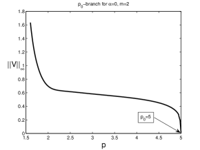
(a) $p_{0}$-branch

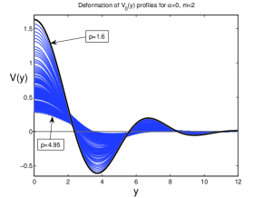
(b) $V_{0}$ profiles

Figure 1. The first $p_{0}$-branch of solutions of (3.1) for $m=2$ and $\alpha=0$; the branch (a) and deformation of profiles $V_{0}(y)$ with $p$, (b).

For $\alpha>0$, the $p$-bifurcation branches can essentially change their topology and can be closed curves, as Figure 2 demonstrates for $\alpha=1$. Here, the first $p_{0}$-branch is initiated at $p_{0}=9$ and has the saddle-node (turning) point at

$$p_{\rm s-n}=3.51...\,.$$

Eventually, the branch ends up at the third critical point (1.6), i.e., at

$$p_{2}=1+\frac{8}{3}=3.666...\,.$$

For convenience, in Figure 3, we give the enlarged structure of the almost vertical part of the branch in Figure 2(a) and VSS profiles on it for $p\in[p_{\rm s-n},p_{2}]$.

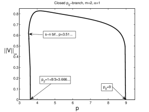
(a) $p_{0}$-branch

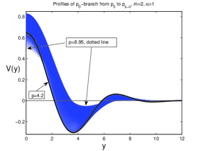
(b) $V_{0}$ profiles

Figure 2. The closed $p_{0}$-branch of solutions of (3.1) for $m=2$, and $\alpha=1$; the branch (a) and deformation of profiles $V_{0}(y)$, (b).

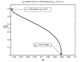
(a) $p_{0}$-branch

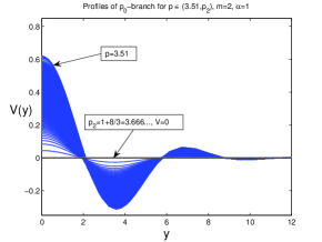
(b) $V_{0}$ profiles

Figure 3. The $p_{0}$-branch of solutions of (3.1) between two bifurcations; $p\in[3.51,3.66]$, $m=2$, $\alpha=1$; the branch (a) and deformation of profiles $V_{0}(y)$, (b).

3.2. On $\alpha$-branches for fixed $p$

A typical example is presented in Figure 4, where we show the first $\alpha$-branch for $N=1$, $p=2$, that, according to (1.7), is originated at the bifurcation point

$$\alpha_{0}=-\frac{3}{4}\quad(l=0).$$

We observe from (b) that the profiles get wider as $\alpha$ increases. This is a natural phenomenon that will play an important role in what follows. It should be noted that Figure (b) does not explain jump-discontinuities that are not only possible but often happen in such numerics (in view of huge density of various branches of solutions), and were observed even with the enhanced Tolerances $10^{-4}$ and the step $\Delta\alpha=10^{-3}$. In fact, (a) shows for $\alpha\approx 1$ a certain non-smoothness of the branch that we cannot explain. To be honest, we cannot guarantee that here this is not associated with a discontinuous jump to other neghbouring branches. The $\alpha$-branching deserves both extra numerical and analytical study.

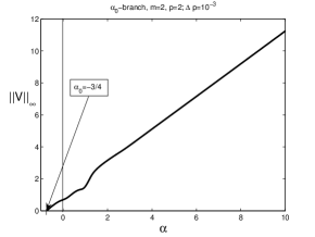
(a) $\alpha_{0}$-branch

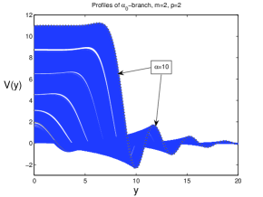
(b) $V_{0}$ profiles

Figure 4. The first $\alpha_{0}$-branch of solutions of (3.1) for $m=2$, and $p=2$; the branch (a) and deformation of profiles $V_{0}(y)$, (b).

3.3. Further bifurcations and discussion

We denote the basic set of VSS profiles by

(3.5) $$\mbox{basic spectrum:}\quad V_{0},\,\,V_{1},\,\,V_{2},\,...,\,V_{k},\,...\,.$$

Each $V_{k}(y)$ satisfies the approximate Sturmian property, i.e., has precisely $k$ dominant extrema. For $m=1$, this is true sharply, by the Maximum Principle. For $m\geq 2$, by “dominant” we mean those minima or maxima that are different from smaller ones in the oscillatory tail of the solutions. This approximate Sturm’s zero (extremum) property for $N=1$ is associated with the fact that in the ODE (1.4) with $m\geq 2$, the leading $2m$th-order operator is a multiplication of $m$ positive second-order ones,

$$-(-1)^{m}D_{y}^{2m}\equiv-(-D_{y}^{2})^{m},$$

for which Sturm’s property is true concerning its eigenfunctions; see general conclusions in Ellias [11], also applications to bifurcation diagrams of interest here in [1, 29]. It turns out that lower-order perturbations in (1.4) create only sufficiently small extrema and infinitely many zeros in the exponential tails of solutions.

For $\alpha>0$, the basic profiles are essentially deformed. For instance, a few of such profiles (already available in Figure 4(b)) are shown in Figure 5 for various $\alpha\geq 0$.

A principal new feature of the problem with the exponent $\alpha$ is that there may occur other saddle-node bifurcations in the ODE in (3.1). The origin of extra $\alpha$-bifurcations can be seen as follows. The leading operator in (1.4),

$$\tilde{\bf B}V=-(-\Delta)^{m}V-|V|^{p-1}V$$

is coercive and negative in the topology of the Sobolev space $H^{2m}(B_{l})\cap L^{p+1}(B_{l})$ in the subcritical range (2.15) (this is enough for $N=1$). Here $B_{l}$ is the ball of the radius $l>0$ in ${\mathbb{R}}^{N}$. It follows from Lemma 2.1(i) that a similar result remains true in the weighted space $L^{2}_{\rho}({\mathbb{R}}^{N})$, and moreover, the first linear term $\frac{1}{2m}\,y\cdot\nabla V$ can be estimated via the leading operator. We then observe that the crucial part is played by the second term

$$\beta V\equiv\frac{1+\alpha}{p-1}\,V.$$

The multiplier $\frac{1+\alpha}{p-1}$ gets arbitrarily large positive for $\alpha\gg 1$, and hence can produce a bifurcation, where the negative and positive operators are sufficiently balanced; see more precise estimates below.

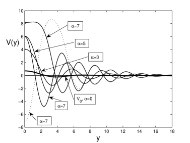
Figure 5. Various VSS profiles associated with the first basic pattern $V_{0}(y)$ for $p=2$, $N=1$, and different values of $\alpha\in[0,7]$.

Let us discuss THE numerical evidence more systematically. In Figure 6, we show the first VSS profiles $V_{0}(y)$ satisfying (1.4) for $p=3$, $N=1$, and for a number of different values of $\alpha$. The bold line corresponds to $V_{0}$ in the classic case $\alpha=0$ studied in [19].

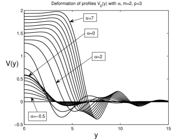
Figure 6. Deformation with $\alpha$ of the first profile $V_{0}(y)$ of (3.1), with $p=3$, for $\alpha\in[-0.5,7]$.

In Figure 7, we show twelve different even VSS profiles $V_{2k}(y)$ for $p=2$, $N=1$, and $\alpha=4$. Note that according to critical exponents (1.7), there exist precisely ten critical values below 4, at which such profiles can be originated,

$$\alpha_{0}=-\frac{3}{4},\,\,\alpha_{2}=-\frac{1}{4},\,\,\alpha_{4}=\frac{1}{4},\,\,...\,\,,\,\alpha_{16}=\frac{13}{4},\,\,\alpha_{18}=\frac{15}{4}.$$

On the other hand, according to (1.6), there exist the same number of critical exponents $p_{l}$ that are above 2,

$$p_{0}=21,\,\,p_{2}=\frac{23}{3},\,\,...\,\,,\,p_{16}=\frac{37}{17},\,\,p_{18}=\frac{39}{19}.$$

It follows that at least two profiles in Figure 7 are not generated by standard $p$- or $\alpha$-curves originated at bifurcation points. This mystery remains an open problem and needs extra analysis. We expect that some pairs of these profiles could be originated at saddle-node bifurcations at some $\alpha_{\rm s-n}>0$. It is seen that the profiles slightly “oscillate” about the constant equilibrium of the ODE in (3.1) which is

$$V_{+}=\bigl{(}\frac{1+\alpha}{p-1}\bigr{)}^{\frac{1}{p-1}}=5\quad\mbox{for \, $p=2$ \, and \, $\alpha=4$}.$$

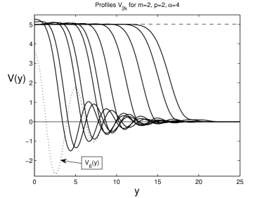
Figure 7. Twelve even VSS profiles $V_{2k}(y)$ for $p=2$, $N=1$, and $\alpha=4$.

For convenience, below we present the standard multiplicity result for the autonomous case. In Figure 8, we show first three solutions $V_{0}(y)$, $V_{1}(y)$, and $V_{2}(y)$ of the problem (3.1) with $p=1.5$ and $\alpha=0$. As was shown in [19], these $p$-bifurcation branches exhaust the whole set of VSS profiles in the case $\alpha=0$. Notice that the mutual geometry of VSS profiles in the case $\alpha=0$ essentially differs from that in Figure 7.

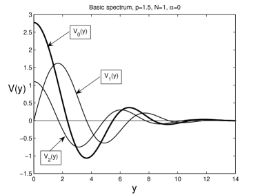
Figure 8. Three VSS profiles $V_{0}$, $V_{1}$, and $V_{2}$ for $\alpha=0$; $p=1.5$ and $N=1$.

Let us more clearly show that, for $\alpha>0$, there occur other bifurcation-branching phenomena. In Figures 9 and 10, we again consider the case $p=1.5$, $N=1$, and $\alpha=7$. For this sufficiently large $\alpha$, according to (1.7), we observe several profiles from the basic family $\{V_{2k}\}$ of even functions that are now concentrated about the constant equilibrium. Namely, in Figure 9, we show nine profiles $\{V_{2k}\}$. Figure 10 demonstrates thirteen odd profiles from the family $\{V_{2k+1}\}$. In this case, instead of symmetry conditions (3.3), we take the anti-symmetry ones (3.4). Then the solutions $V(y)$ are continued in the odd manner, $V(-y)\equiv-V(-y)$ for $y<0$.

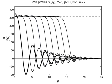
Figure 9. Several VSS profiles $V_{2k}(y)$ from satisfying (3.1) for $p=1.5$ and $\alpha=7$.

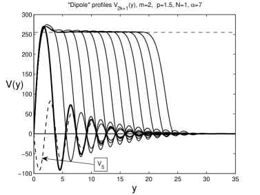
Figure 10. Several odd VSS profiles $V_{2k+1}(y)$ satisfying (3.1) for $p=1.5$ and $\alpha=7$.

Before performing some easy preliminary estimates, we show in Figure 11 the case $p=4$ and $\alpha=10$, where a similar set of seven VSS patterns from the even family $\{V_{2k}\}$ are presented. In addition, we see here another new family

(3.6) $$\{V_{\sigma_{1}}\},\quad\mbox{with multiindex}\quad\sigma_{1}=\{+0,1,-k\},$$

where $0,1$, and $k$ in $\sigma_{1}$ stand for an “effective number of intersections” of the profiles with three consecutive equilibria $V_{+},0$, and $-V_{+}$. We will discuss this new family later on.

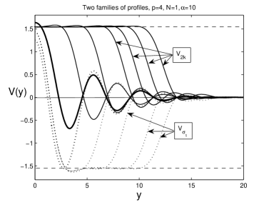
Figure 11. VSS profiles from $\{V_{2k}\}$ and $\{V_{\sigma_{1}}\}$ for $p=4$, $N=1$, and $\alpha=10$.

In Figure 12, we show the basic profiles $V_{2k}(y)$ and others for $m=p=2$ and $\alpha=10$. This computation is important to treat the results in Figure 4 on the $\alpha$-branches.

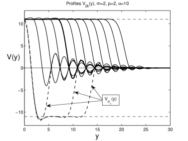
Figure 12. Profiles from the family $\{V_{2k}\}$ for $m=p=2$, $N=1$, and $\alpha=10$.

For future convenience, some of the results are natural to present for the rescaled equation by using the scaling

(3.7) $$V\mapsto CV,\quad y\mapsto cy,\quad\mbox{where}\quad C^{p-1}=\beta,\,\,\,c=C^{\frac{p-1}{2m}}=\beta^{\frac{1}{2m}},$$

that gives the following rescaled ODE:

(3.8) $$(-1)^{m+1}V^{(2m)}+\frac{1}{\beta}\,\frac{1}{2m}\,yV^{\prime}+V-|V|^{p-1}V=0.$$

The constant equilibria are now fixed and are independent of the parameters,

(3.9) $$V_{\pm}=\pm 1\quad(\mbox{and}\,\,\,V=0),$$

so we do not observe such huge VSS profiles as, for instance, in Figure 9. The corresponding rescaled families $\{V_{2k}\}$ and $\{V_{\sigma_{1}}\}$ for $m=2$, $p=1.5$, and $\alpha=7$ are shown in Figure 13(a) and (b). Figure 14 shows another more complicated family of even VSS profile

$$V_{\sigma_{2}}(y),\quad\mbox{where}\quad\sigma_{2}=\{+1,1,-2,1,+k\}.$$

By boldface dotted line we denote therein a different profiles from the family $\{V_{\sigma_{3}}\}$, with a distinct multiindex $\sigma_{3}=\{-0,1,+2,1,-k\}$. It seems that there are other families of VSS profiles with more involved geometric structures that are very difficult to catch numerically, so we stop the discussion at this moment.

We expect that all the new profiles from families $\{V_{\sigma_{1}}\}$, $\{V_{\sigma_{2}}\}$, etc., are originated at saddle-node bifurcations at some $\alpha_{\sigma_{j}}>0$ and cannot be extended to $\alpha=0$. Recall that such VSS solutions were not detected in the autonomous case $\alpha=0$, [19]. Numerics with $\Delta\alpha=10^{-3}$ show some evidence concerning this though are also rather unstable demonstrating typical jumps between many neighbouring $\alpha$-branches. We believe that such stable jumps definitely show existence of saddle-node points that are difficult to detect numerically.

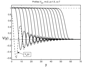
(a) profiles $V_{2k}$

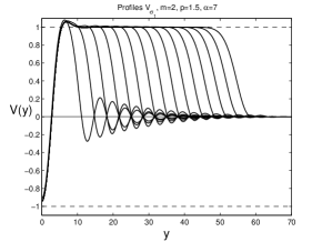
(b) profiles $V_{\sigma_{1}}$

Figure 13. Two different families of VSS profiles for $m=2$, $p=1.5$, $N=1$, and $\alpha=7$.

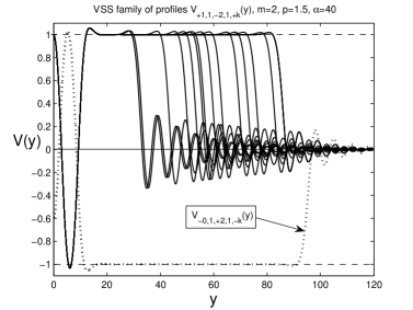
Figure 14. Some profiles from the family $\{V_{\sigma_{2}}\}$ for $m=2$, $p=1.5$, and $\alpha=40$.

On countable sets via shooting arguments. As an illustration, consider the ODE in (3.1) (i.e., for $m=2$ and $N=1$) in the symmetric case (3.3), so we study $V_{2k}$ and other even profiles. The shooting argument justifies existence of a connection of the 2D bundle near the origin, which is characterized by two symmetry conditions (3.3), so that the bundle has two parameters

(3.10) $$f(0)\quad\mbox{and}\quad f^{\prime\prime}(0).$$

We then need to intersect this bundle with the exponential bundle at $y=+\infty$, where the linearized ODE admits the following WKBJ-type asymptotics (we omit power-like multipliers that are not important at this stage):

$$V^{(4)}=-\frac{1}{2m}\,V^{\prime}y+...\quad\Longrightarrow\quad V(y)\sim{\mathrm{e}}^{ay^{4/3}},\quad\mbox{with}\,\,\,a^{3}=\frac{1}{4}\big{(}\frac{3}{4}\big{)}^{3}.$$

Therefore, there exists a 1D unstable bundle with positive $a_{0}=\frac{3}{4}\,4^{-1/3}$, and a 2D stable oscillatory bundle with

$$a_{\pm}=a_{0}\big{(}-\frac{1}{2}\pm{\mathrm{i}}\frac{\sqrt{3}}{2}\big{)}\quad\,\,\big{(}{\rm Re}\,a_{\pm}<0\big{)}.$$

Thus, we observe here a typical difficult two-parameter shooting problem of 2D$\to$2D connection of two manifolds. In this case, in the above shooting approach, we arrive at two equations for two parameters given in (3.10). In the analytic case $p=3,5,...$, where the dependence on parameters is assumed to be analytic, we conclude that the set of VSS profiles is at most countable. Moreover, for fixed $p<p_{0}$ and any $\alpha>0$, we expect a finite (but, possibly, arbitrarily large for some values) number of VSS profiles according to the above $p$- and $\alpha$-bifurcations and extra possible $\alpha$-saddle-node bifurcations that much less are known about.

On oscillatory blow-up in the ODE. Here we briefly discuss an important aspect of ODEs such as (1.4), $N=1$ (or in radial geometry). Namely, these admit a strong (nonlinear) unstability of orbits $V(y)$ that is associated not with the exponential growth in the linear setting, but with the blow-up due to the main two terms in the ODE in (3.1). For $m=2$ these are

(3.11) $$V^{(4)}=-|V|^{p-1}V,$$

where we omit all linear terms that are negligible as $|V|\to+\infty$. Obviously, (3.11) does not admit blow-up solutions of constant sign, so we need to describe the oscillatory blow-up. In Figure 15, we present typical blow-up behaviour of solutions $\ln|V(y)|$ of (3.11) for $y>0$ with Cauchy data

$$V(0)=1,\quad V^{\prime}(0)=V^{\prime\prime}(0)=V^{\prime\prime\prime}(0)=0.$$

Solutions blow-up at some finite $y_{0}>0$ with definite oscillatory behaviour as $y\to y_{0}$.

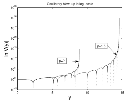
Figure 15. Oscillatory blow-up for the ODE (3.11) for $p=\frac{3}{2}$ and $p=2$.

In order to detect this oscillatory behaviour, by shifting $y_{0}-y\mapsto-y$, we have that blow-up happens at $y=0$, i.e., as $y\to 0^{-}$, and introduce the oscillatory component $\varphi(s)$ as follows:

(3.12) $$V(y)=(-y)^{\mu}\varphi(s),\quad\mbox{where}\quad s=\ln(-y)\quad\mbox{and}\quad\mu=-\frac{4}{p-1}<0.$$

Then $\varphi(s)$ solves the following autonomous ODE in ${\mathbb{R}}$:

(3.13) $$\begin{matrix}\varphi^{(4)}+2(2\mu-3)\varphi^{\prime\prime\prime}+(6\mu^{2}-18\mu+11)\varphi^{\prime\prime}+2(2\mu^{3}-9\mu^{2}\vskip 3.0pt plus 1.0pt minus 1.0pt\vskip 3.0pt plus 1.0pt minus 1.0pt\cr+\,11\mu-3)\varphi^{\prime}+\mu(\mu-1)(\mu-2)(\mu-3)\varphi=-|\varphi|^{p-1}\varphi.\end{matrix}$$

Obviously, this ODE also admits blow-up singularities as (3.11), but we are interested in bounded or slower growing orbits that can be extended up to the blow-up point $s=-\infty$.

In addition, using a standard min-max scenario of orbits behaviour on parameters, we expect a bounded (hopefully, periodic) or a spiral-type solution $\varphi_{*}(s)$ in ${\mathbb{R}}$ to exist, which, according to (3.12), will describe a generic structure of blow-up singularities. The blow-up instabilities make it very difficult to see necessary orbits of equation (3.13) even numerically. A logarithmic-type distribution of zeros close to blow-up points as in (3.12) is seen in Figure 15.

What is crucial in this case, is that the whole unstable bundle is two-dimensional incorporating the parameter $y_{0}$ as the position of the blow-up point (i.e., $y\mapsto y_{0}-y$ in (3.12)) and the parameter $s_{0}$ of translation, $\varphi_{*}(s)\mapsto\varphi_{*}(s+s_{0})$. Therefore, our VSS profiles are those that have nothing to do with this singular blow-up bundle, so we again observe two equations for two parameters in (3.10).

4. Passing to the limit $\alpha\to\infty$

Without loss of generality, we consider the 1D case in (1.4) and bear in mind the first symmetric similarity profile $V_{0}(y)$ for the ODE

(4.1) $$(-1)^{m+1}V^{(2m)}+\frac{1}{2m}\,yV^{\prime}+\beta V-|V|^{p-1}V=0,\quad\mbox{where}\quad\beta=\frac{1+\alpha}{p-1}\to+\infty$$

as $\alpha\to+\infty$. For $\beta\gg 1$, the first natural step is to use the scaling (3.7) and to write the resulting equation in the perturbed form,

(4.2) $${\bf D}_{\infty}(V)\equiv(-1)^{m+1}V^{(2m)}+V-|V|^{p-1}V=-\frac{1}{\beta}\,\frac{1}{2m}\,yV^{\prime}.$$

Hence, the right-hand side becomes negligible as $\beta\to\infty$ on smooth solutions.

Formally passing to the limit $\beta\to\infty$ in (4.2), we obtain the limit equation

(4.3) $${\bf D}_{\infty}(W)\equiv(-1)^{m+1}W^{(2m)}+W-|W|^{p-1}W=0\quad\mbox{for}\quad y>0,\quad W(+\infty)=0.$$

Let us show that a nontrivial solution of (4.3) does not exist. For instance, for $m=2$,

(4.4) $$\begin{matrix}-W^{(4)}+W-|W|^{p-1}W=0,\quad\mbox{so that, for $y\gg 1$,}\vskip 3.0pt plus 1.0pt minus 1.0pt\vskip 3.0pt plus 1.0pt minus 1.0pt\\ W^{(4)}=W+...\quad\Longrightarrow\quad\exists\,\,1D\,\,\mbox{bundle},\,\,\,W(y)\sim C{\mathrm{e}}^{-y}+...\,.\end{matrix}$$

This 1D is not enough to satisfy two symmetry conditions (3.4). Similarly, for $m=3$,

(4.5) $$\begin{matrix}W^{(6)}+W-|W|^{p-1}W=0,\quad\mbox{and for $y\gg 1$,}\vskip 3.0pt plus 1.0pt minus 1.0pt\vskip 3.0pt plus 1.0pt minus 1.0pt\qquad\quad\\ W^{(6)}=-W+...\quad\Longrightarrow\quad\exists\,\,2D\,\,\mbox{bundle with char. values $\lambda_{\pm}=-\frac{\pi}{6}\pm{\rm i}\,\frac{\sqrt{3}}{2}$}.\qquad\quad\end{matrix}$$

The 2D bundle is not sufficient to satisfy three symmetry conditions at the origin,

$$W^{\prime}(0)=W^{\prime\prime\prime}(0)=W^{(5)}(0)=0.$$

The same lack of dimension happens for any $m\geq 1$. In other words, nonexistence for (4.3) is a typical property.

Such nonexistence is easily checked numerically. In Figure 16, we show for $m=p=2$ that as $\alpha$ increases the VSS profiles with a fixed length of the flat part (such solutions exist) become more and more oscillatory and ceases to exist for $\alpha=+\infty$.

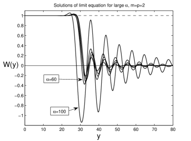
Figure 16. Towards nonexistence for the ODE (4.4), $m=p=2$: solutions of (4.2) get very oscillatory for $\alpha\gg 1$.

On the other hand, profiles with huge flat non-oscillatory parts get very wide for $\alpha\gg 1$. For instance, Figure 17 shows for $p=1.5$ that for $\alpha=40$, the last less oscillatory VSS profile $V_{2k}(y)$ has the flat part of the length $\sim 380$, while the first profiles are strongly oscillatory (and do not admit passage to the limit $\alpha\to\infty$). Notice that according to bifurcation exponents (1.7), for $\alpha=40$, we expect, at least,

164 profiles $$V_{2k} V_{\sigma_{1}}$$ and 164 profiles ,

i.e., 328 VSS profiles overall (and more in view of possible saddle-node bifurcations beforehand, at some $\alpha_{\rm s-n}\in(0,40)$).

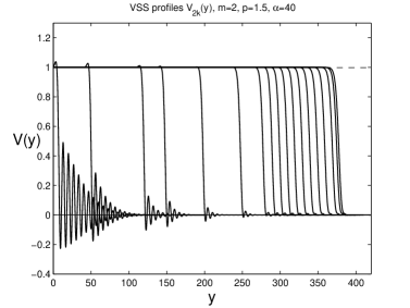
Figure 17. Some VSS profiles satisfying (4.2) for $m=2$, $p=1.5$, and $\alpha=40$.

Therefore, as $\alpha\to+\infty$, one can that the VSS profiles get wider indefinitely in the sense that, in the rescaled variables, uniformly on bounded intervals,

(4.6) $$V_{0}(y)\to 1\quad\mbox{as}\quad\alpha\to+\infty,$$

and the divergence is sufficiently (exponentially) fast.

As a simple illustration of this behaviour presented in Figure 17, we give a nonexistence result concerning a step-like profile for the limit equation (4.4). Assume that, unlike (4.6), there exists a nontrivial finite limit as $\alpha\to\infty$, so (4.4) admits solution $W(y)$ with exponential decay such that

(4.7) $$W(y)\approx 1\quad\mbox{for}\quad y\in[0,L],\,\,\,\mbox{with some}\,\,\,L\gg 1,$$

and that the internal layer at $y\sim L$ does not depend essentially on $L$ (recall that (4.4) is an autonomous ODE), and, in a natural sense,

(4.8) $$\int_{L}^{\infty}W^{2}\ll L\quad\mbox{and}\quad\int_{L}^{\infty}|W|^{p+1}\ll L.$$

The following nonexistence result has a “conditional” nature, where we prohibit certain solutions of a specific spatial shape:

Proposition 4.1.

The ODE $(\ref{e1})$ does not admit a nontrivial solution with exponential decay at infinity satisfying $(\ref{WW1})$ and $(\ref{WW2})$.

Proof. We use two identities obtained by multiplying (4.4) in $L^{2}$ by $W$ and $yW^{\prime}$ (Pohozaev’s multiplier in elliptic theory, [28]) to get

(4.9) $$\left\{\begin{matrix}-\int(W^{\prime\prime})^{2}+\int W^{2}-\int|W|^{p+1}=0,\qquad\quad\vskip 3.0pt plus 1.0pt minus 1.0pt\vskip 3.0pt plus 1.0pt minus 1.0pt\\ -\frac{3}{2}\int(W^{\prime\prime})^{2}-\frac{1}{2}\int W^{2}+\frac{1}{p+1}\int|W|^{p+1}=0.\end{matrix}\right.$$

Substituting $\int(W^{\prime\prime})^{2}$ from the first into the second identity yields

(4.10) $$\int W^{2}=\gamma_{0}\int|W|^{p+1},\quad\mbox{where}\quad\gamma_{0}=\frac{3p+5}{4(p+1)}.$$

Since $\gamma_{0}<1$ for any $p>1$, this contradicts hypotheses (4.7), (4.8) under which both integrals in (4.10) are close to $L$. ∎

5. On some VSSs results for the non-monotone absorption

In this short section, we orient our nonexistence business to the following PDE:

(5.1) $$u_{t}=-(-\Delta)^{m}u-t^{\alpha}|u|^{p},$$

where, unlike (1.1), we take the non-monotone absorption nonlinearity $|u|^{p}$.

5.1. On local existence close to bifurcation points

Local existence of similarity solutions for $p<p_{0}$ for equation (1.4), where

(5.2) $$|V|^{p-1}V\mapsto|V|^{p},$$

can be established as above by bifurcation theory. Then, for several types of “positively dominant” VSS profiles $V(y)$ as in Figures 7, 9, 10, 12, and 13(a), their structure changes slightly after the replacement (5.2).

For instance, in Figure 18, we present even VSS profiles for the ODE

(5.3) $$-V^{(4)}+\frac{1}{4}\,yV^{\prime}+\beta V-|V|^{p}=0\quad\mbox{in}\quad{\mathbb{R}}\quad\big{(}\beta=\frac{1+\alpha}{p-1}\big{)},$$

in the case $p=1.5$, $\alpha=7$, where most of the solutions are very close to those in Figure 13(a). Excluding first sufficiently small profiles, all the others are clearly positively dominant (the last ones look “almost” positive; careful checking shows that all of them remain oscillatory). Small solutions (dotted lines as well as that of order $\sim 2\cdot 10^{-2}$ given by the solid line) become essentially different. Instead of (3.9), equation (5.3) admits the single constant non-zero equilibrium

(5.4) $$V_{+}=+1\quad(\mbox{and}\,\,\,V_{0}=0),$$

so that VSS profiles $V_{\sigma_{1}}$ such as in Figure 11 and 12 are impossible. Since (5.4) means that for the nonlinearity $-|V|^{p}$, two equilibria $-1$ and 0 just coincide (in fact, identified), we obtain another but similar family of profiles again denoted by $\{V_{\sigma_{1}}\}$ that are shown in Figure 19. For large $\alpha=40$, step-like solutions of (5.3) are practically indistinguishable from those in Figure 17, so that this behaviour as $\alpha\to+\infty$ suits both monotone and non-monotone absorption terms.

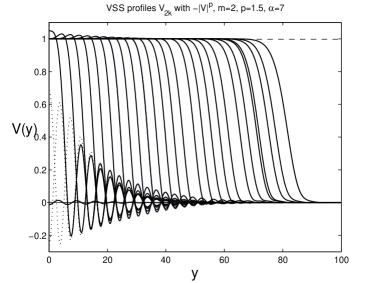
Figure 18. Twenty nine VSS solutions $V_{2k}(y)$ of (5.3) for $m=2$, $p=1.5$, $\alpha=7$.

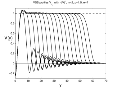
Figure 19. Seventeen VSS solutions $V_{\sigma_{1}}(y)$ of (5.3) for $m=2$, $p=1.5$, and $\alpha=7$.

On the contrary, nonexistence of VSSs for

(5.5) $$p\geq p_{0}=1+\frac{2m(1+\alpha)}{N}$$

can be proved much easier than for the original PDE (1.1). This is explained in detail in [17] for $\alpha=0$, so we present here a few nonexistence comments.

5.2. On nonexistence of similarity profiles

The similarity solutions remain the same, (1.3), with the elliptic equation (1.4), where we use the replacement (5.2). Therefore, integrating this equation over ${\mathbb{R}}^{N}$ with the condition of exponential decay, we obtain in particular that

(5.6) $$\int|V|^{p}=0\quad\mbox{for}\quad p=p_{0}\quad\Longrightarrow\quad V=0.$$

Therefore, all the continuous $p$-branches do not cross the vertical line $p=p_{0}$, so that in the parameter region $\{p\geq p_{0}\}$ there are no VSS profiles at all.

Obviously, for the original equation (1.4) this analysis leads to

(5.7) $$\int|V|^{p-1}V=0\quad\mbox{for}\quad p=p_{0},$$

which is not that controversial. Of course, this prohibits clearly positively dominant VSS profiles such as those in Figure 13(a), but not obvious for profiles having essential negative parts as in (b) therein. Nevertheless, one can see that, for all these profiles, (5.7) is valid, since these are also positively dominant.

5.3. Nonexistence for the PDE

Using a slight modification of the statement and the proof in [17, § 2] based on Pohozaev’s nonlinear capacity approach (see details and related references therein), we formulate the following nonexistence result for (5.1):

Theorem 5.1.

Let $\alpha>-1$ and

(5.8) $$p\geq p_{0}=1+\frac{2m(1+\alpha)}{N}.$$

If a function $u(x,t)\in L^{p}_{\rm loc}({\mathbb{R}}^{N}\times{\mathbb{R}}_{+}\setminus\{(0,0)\})$ satisfies $(\ref{31})$ and $(\ref{g15})$ in the weak sense, then $u=0$.

In particular, this means that, for this nonlinearity, any similarity problem such as (1.4) does not admit a nontrivial solution. Of course, this implies that no other, non-similarity, VSSs exist. For the monotone nonlinearity as in (1.4), the proof of nonexistence gets more involved, and can be done, with some technical changes, along the lines in [17, § 3.2].

Acknowledgement. The author thanks A.E. Shishkov for drawing his attention to time dependent absorption phenomena.

References

- [1] R. Bari and B. Rynne, Solution curves and exact multiplicity results for th order boundary value problems, J. Math. Anal. Appl., 292 (2004), 17–22.
- [2] M. Berger, Nonlinearity and Functional Analysis, Acad. Press, New York, 1977.
- [3] M.S. Birman and M.Z. Solomjak, Spectral Theory of Self-Adjoint Operators in Hilbert Space, D. Reidel, Dordrecht/Tokyo, 1987.
- [4] H. Brezis and A. Friedman, Nonlinear parabolic equations involving measures as initial conditions, J. Math. pures appl., 62 (1983), 73–97.
- [5] H. Brezis, L.A. Peletier, and D. Terman, A very singular solution of the heat equation with absorption, Arch. Rat. Mech. Anal., 95 (1986), 185–209.
- [6] C.J. Budd, V.A. Galaktionov, and J.F. Williams, Self-similar blow-up in higher-order semilinear parabolic equations, SIAM J. Appl. Math., 64 (2004), 1775–1809.
- [7] E.A. Coddington and N. Levinson, Theory of Ordinary Differential Equations, McGraw-Hill Book Company, Inc., New York/London, 1955.
- [8] K. Deimling, Nonlinear Functional Analysis, Springer-Verlag, Berlin/Tokyo, 1985.
- [9] Yu.V. Egorov, V.A. Galaktionov, V.A. Kondratiev, and S.I. Pohozaev, Asymptotic behaviour of global solutions to higher-order semilinear parabolic equations in the supercritical range, Adv. Differ. Equat., 9 (2004), 1009–1038.
- [10] S.D. Eidelman, Parabolic Systems, North-Holland Publ. Comp., Amsterdam/London, 1969.
- [11] U. Ellias, Eigenvalue problems for the equation , J. Differ. Equat., 29 (1978), 28–57.
- [12] M. Escobedo and O. Kavian, Variational problems related to self-similar solutions of the heat equation, Nonlinear Anal., TMA, 11 (1987), 1103–1133.
- [13] A. Friedman, Partial Differential Equations, Robert E. Krieger Publ. Comp., Malabar, 1983.
- [14] V.A. Galaktionov, On higher-order semilinear parabolic equations with measures as initial data, J. Eur. Math. Soc., 6 (2004), 193–205.
- [15] V.A. Galaktionov, S.P. Kurdyumov, and A.A. Samarskii, On asymptotic “eigenfunctions” of the Cauchy problem for a nonlinear parabolic equation, Math. USSR Sbornik, 54 (1986), 421–455.
- [16] V.A. Galaktionov and A.E. Shishkov, Saint-Venant’s principle in blow-up for higher-order quasilinear parabolic equations, Proc. Roy. Soc. Edinburgh, 133A (2003), 1075–1119.
- [17] V.A. Galaktionov and A.E. Shishkov, Higher-order quasilinear parabolic equations with singular initial data, Comm. Contemp. Math., 8 (2006), 331–354.
- [18] V.A. Galaktionov and J.L. Vazquez, A Stability Technique for Evolution Partial Differential Equations. A Dynamical Systems Approach, Birkhäuser, Boston/Berlin, 2004.
- [19] V.A. Galaktionov and J.F. Williams, On very singular similarity solutions of a higher-order semilinear parabolic equation, Nonlinearity, 17 (2004), 1075–1099.
- [20] I.C. Gokhberg and M.G. Krein, Introduction to the Theory of Linear Nonselfadjoint Operators, Transl. Math. Monogr., Vol. 18, AMS, Providence, RI, 1969.
- [21] S. Kamin and L.A. Peletier, Singular solutions of the heat equation with absorption, Proc. Amer. Math. Soc., 95 (1985), 205–210.
- [22] S. Kamin and L.A. Peletier, Large time behaviour of solutions of the porous media equation with absorption, Israel J. Math., 55 (1986), 129–146.
- [23] S. Kamin and L. Véron, Existence and uniqueness of the very singular solution of the porous media equation with absorption, J. Analyse Math., 51 (1988), 245–258.
- [24] M.A. Krasnosel’skii, Topological Methods in the Theory of Nonlinear Integral Equations, Pergamon Press, Oxford/Paris, 1964.
- [25] M.A. Krasnosel’skii and P.P. Zabreiko, Geometrical Methods of Nonlinear Analysis, Springer-Verlag, Berlin/Tokyo, 1984.
- [26] M. Marcus and L. Veron, Initial trace of positive solutions to semilinear parabolic inequalities, Adv. Nonlinear Studies, 2 (2002), 395–436.
- [27] V.G. Maz’ja, Sobolev Spaces, Springer-Verlag, Berlin/Tokyo, 1985.
- [28] S.I. Pohozaev, Eigenfunctions of the equation , Soviet Math. Dokl., 6 (1965), 1408–1411.
- [29] B. Rynn, Global bifurcation for th-order boundary value problems and infinitely many solutions of superlinear problems, J. Differ. Equat., 188 (2003), 461–472.
- [30] J. Shi and J. Wang, Morse indices and exact multiplicity of solutions to semilinear elliptic problems, Proc. Amer. Math. Soc., 127 (1999), 3685–3695.
- [31] A.E. Shishkov and L. Véron, Singular solutions of some nonlinear parabolic equations with spatially inhomogeneous absorption, Calc. Var. PDEs, 33 (2008), 343–375.
- [32] M.E. Taylor, Partial Differential Equations III. Nonlinear Equations, Springer, New York/Tokyo, 1996.
- [33] M.A. Vainberg and V.A. Trenogin, Theory of Branching of Solutions of Non-Linear Equations, Noordhoff Int. Publ., Leiden, 1974.