Excitation of standing kink oscillations in coronal loops

Abstract

In this work we review the efforts that have been done to study the excitation of the standing fast kink body mode in coronal loops. We mainly focus on the time-dependent problem, which is appropriate to describe flare or CME induced kink oscillations. The analytical and numerical studies in slab and cylindrical loop geometries are reviewed. We discuss the results from very simple one-dimensional models to more realistic (but still simple) loop configurations. We emphasise how the results of the initial value problem complement the eigenmode calculations. The possible damping mechanisms of the kink oscillations are also discussed.

1 Introduction

Transversal coronal loop oscillations are regularly observed by the EUV telescope on board $TRACE$. Nowadays, there is abundant information about the period, damping time and amplitude of the oscillations (see for example Aschwanden et al., 2002; Schrijver et al., 2002, and see also the review of M. Aschwanden in this volume). In most of the cases these oscillations are triggered by a flare or a CME, and they have been interpreted as fast standing magnetohydrodynamic (MHD) kink oscillations of cylindrical tubes (see Nakariakov and Ofman, 2001; Ruderman and Roberts, 2002; Goossens et al., 2002).

In general, most of the theoretical studies on loop oscillations assume that the system is in the stationary state and that the loop dynamics is given by the normal modes. The calculation of the eigenmodes is possible in rather simple configurations but their properties are usually unknown in complex structures. Although normal modes should be seen as the building blocks to interpret coronal loop oscillations they do not represent the whole picture, but their study provides a basis for understanding the dynamics of the system. To have a more accurate description, the time-dependent problem needs to be analysed. Ideally, we would like to know which normal modes are excited given an initial perturbation.

Although there is an extensive literature about MHD oscillations in coronal loops only those theoretical works where the time-dependent analysis has been considered are reviewed here. Usually the time-dependent problems are classified in driven or in initial-value problems. Driven problems are useful to model, among others, the effect of the photospheric motions in coronal loops. In this case a continuous motion is applied at the base of the loop exciting several kinds of modes that propagate along the tube. On the other hand, initial-value problems are more appropriate to describe a sudden release of energy, as in flares. Such energy release generates a disturbance, a blast wave or an EIT wave, that propagates in the corona and produces kink oscillations of nearby loops. In this work we will concentrate on initial-value problems. Moreover, since most of the observations of kink oscillations are interpreted as the fundamental standing kink mode, here we will focus only on this mode, characterised by a single frequency and a dominant wavenumber along the loop. For propagating kink modes, characterised by a wide superposition of different longitudinal wavenumbers and frequencies, the reader is referred to the works of Murawski and Roberts (1993a, b, 1994); Huang et al. (1999); Selwa and Murawski (2004); Ogrodowczyk and Murawski (2006, 2007) in slab models and to Roberts et al. (1983, 1984); Selwa et al. (2004); Terra-Homem et al. (2003) in cylindrical loops.

In this work we first describe the results of the time-dependent problem starting with simple loop models and then we increase the complexity of the equilibrium. We also centre on those studies where a direct comparison with eigenmodes can be done since this helps to understand and interpret the results of the time-dependent problems.

2 Basic Loop Models

Two basic equilibrium models have been studied in detail in the literature. They are the simplest representation of coronal loops and are important to understand the basic properties of MHD waves. These models are the slab and the cylindrical flux tube.

2.1 Slab

The simplest loop model is a Cartesian slab configuration. In this model the loop is represented by a plasma column of enhanced density, $\rho_{\rm i}$, respect to the coronal environment, with density $\rho_{\rm e}$. The slab has a half-width of $a$ and the magnetic field is vertical (${\bf B}=B_{0}{\bf e}_{z}$). Since the inhomogeneity is in one direction, hereafter assumed in $x$, it is possible to make Fourier analysis in the other ignorable directions ($y$ and $z$). The reader is referred to Edwin and Roberts (1982) and Terradas et al. (2005a) (with special attention to the leaky modes) for the details about the dispersion diagram in this model. When the wave propagation is in the plane of the slab then the frequency of the fundamental fast kink body mode, in the limit of thin tubes (when $k_{z}a\ll 1$), tends to the external Alfvén frequency,

$$\omega=k_{z}\,v_{\rm Ae},$$ (1)

where $v_{\rm Ae}=B_{0}/\sqrt{\mu\rho_{\rm e}}$ is the external Alfvén speed. However, when the perpendicular propagation is allowed ($k_{y}\neq 0$) the body kink mode is transformed in a surface wave (see Zhelyazkov et al., 1996; Arregui et al., 2007) and its frequency tends to the kink frequency (when $k_{y}\gg k_{z}$)

$$\omega_{k}=k_{z}\sqrt{\frac{\rho_{\rm i}v_{\rm Ai}^{2}+\rho_{\rm e}v_{\rm Ae}^{2}}{\rho_{\rm i}+\rho_{\rm e}}}.$$ (2)

In general this model is appropriate if the structure is invariant in the perpendicular plane (i.e. in the $y-$direction).

2.2 Cylinder

A cylindrical flux tube is the natural extension of the previous model. The reader is referred to Edwin and Roberts (1983); Cally (1986, 2003) for the details of the dispersion diagram and the classification of the different modes (trapped and leaky). Here we will restrict to body waves and the $m=1$ mode (the oscillation that displaces transversally the whole tube). In the limit of thin tube the frequency of oscillation is the kink frequency, given by equation (2).

The main advantage of the cylindrical model is that it represents a three-dimensional structure. It is interesting to note that the kink body modes are very similar to the kink modes of the slab model when $k_{y}$ is large. The frequency of oscillation is the same, the kink frequency, and the eigenfunction is quite localised near the loop boundary. In fact in some papers (see for example Hollweg and Yang, 1988), the results of the slab models have been extended to the cylindrical geometry by using the equivalent of the azimuthal wavenumber in Cartesian coordinates, i.e. assuming that $k_{y}=m/R$.

On the other hand, one of the assumptions that is usually relaxed in the cylindrical and in the slab model is the Alfvén speed profile across the boundary. In the simple models it is assumed that the density (and the Alfvén speed) has a discontinuous jump at the interface between the loop and the coronal environment. However, if the Alfvén speed has an inhomogeneous layer, with a typical width of $l$, then the process of resonant absorption takes place (for $m\geq 1$ in the cylindrical model or for $k_{y}\neq 0$ in the slab model).

2.3 Curved configurations

One of the configurations that takes into account the curvature, neglected in the previous models is the circular loop model. In this force-free model the shape of the magnetic field lines is given by a purely poloidal magnetic field,

$$B_{\theta}=B_{0}\frac{r_{0}}{r}.$$ (3)

The density profile is usually chosen (in the zero-$\beta$ approximation) to have the same dependence as the magnetic field and with a density enhancement, representing the loop, at a given radius. The advantages of this model is that it is possible to make Fourier analysis along the $\theta-$direction and the loop cross section is constant along the tube. One of the disadvantages is that it has a singularity at $r=0$ and this might be difficult to handle from the numerical point of view.

Another popular model is the potential arcade. In this model the current-free magnetic field is given by

$$B_{x}=B_{0}\sin\left(x/\Lambda_{B}\right)\,e^{-z/\Lambda_{B}},$$ (4)

$$B_{z}=-B_{0}\cos\left(x/\Lambda_{B}\right)\,e^{-z/\Lambda_{B}},$$ (5)

where $\Lambda_{B}=L/\pi$ and $L$ is the arcade width. The background density is usually taken to be of the form

$$\rho=\rho_{0}\,e^{-z/\Lambda}.$$ (6)

The parameter $\Lambda$ allows to have a decreasing or increasing Alfvén speed with height ($v_{\rm A}$ is independent of the $x-$coordinate) and the loop is modelled by a density enhancement along certain field lines. The configuration is well behaved at the origin but the loop cross section is not constant along the tube and no Fourier analysis is allowed along the field lines.

These two equilibrium models are two-dimensional but they can still be used to study curved loops in three dimensions assuming that the field is invariant in the perpendicular direction to the plane. Other sophisticated equilibrium models involve three-dimensional dipoles or even photospheric magnetic field extrapolations, usually force free, together with the inclusion of a certain density profile along the field lines. However, these models are still in a very primitive stage.

3 Waves in Slabs

3.1 Basic properties of fast MHD waves in a uniform line-tied medium

We start with the most simple configuration, a uniform plasma permeated by a vertical and uniform magnetic field. In the $\beta$ zero limit the ideal linearised MHD equations reduce to the well-known wave equation for the fast modes,

$$\frac{\partial^{2}\xi}{\partial{t^{2}}}=v^{2}_{A}\left(\frac{\partial^{2}\xi}{\partial{x^{2}}}+\frac{\partial^{2}\xi}{\partial{z^{2}}}\right),$$ (7)

where $\xi$ is the horizontal displacement and $v_{\rm A}=B_{0}/\sqrt{\mu\rho}$ is the Alfvén speed. Since $\beta=0$ slow modes and Alfvén waves (we assume that $k_{y}=0$) are absent. We Fourier analyse in the $z$-direction, i.e. we assume that the perturbations are of the form $e^{-ik_{z}z}$. Hence, equation (7) reduces to the Klein-Gordon equation,

$$\frac{\partial^{2}\xi}{\partial{t^{2}}}=v^{2}_{A}\frac{\partial^{2}\xi}{\partial{x^{2}}}-\omega_{\rm c}^{2}\xi,$$ (8)

where $\omega_{\rm c}=v_{\rm A}k_{z}$ is the cut-off frequency. Thus, after introducing the longitudinal wavenumber $k_{z}$ the two-dimensional wave equation reduces to a one-dimensional equation, and by selecting the appropriate value of this parameter the effect of line-tying can be easily incorporated. For the fundamental oscillation with a node at each footpoint we have that $k_{z}=\pi/L$, $L$ being the length of the system (or loop if we include a density enhancement) in the vertical direction. In this model the time a wave needs to travel along the entire loop to feel the effect of the photosphere is neglected, and the loop instantly feels the effect of line-tying.

Normal mode solutions of equation (8), i.e. with a dependence of the form $e^{i(\omega t-kx)}$, yield the dispersion relation $\omega=\sqrt{k^{2}v_{\rm A}^{2}+\omega_{\rm c}^{2}}$ which indicates that wave propagation is dispersive. The propagation speed for waves with wavenumber $k$ is the group velocity,

$$v_{g}=\frac{d\omega}{dk}=\frac{k\,v_{\rm A}^{2}}{\sqrt{k^{2}v_{\rm A}^{2}+\omega_{\rm c}^{2}}}=\frac{\sqrt{\omega^{2}-\omega_{\rm c}^{2}}}{\omega}\,v_{\rm A},$$ (9)

which ranges between zero, for waves with infinite wavelength, and $v_{\rm A}$ for waves with infinitely small wavelength. Therefore, modes with short wavelengths propagate faster than modes with larger wavelengths. In addition, any mode with frequency below the cut-off frequency is evanescent and unable to propagate in the medium. The dispersive behaviour of waves is simply due to the fact that we assume a fixed wavelength along the loop (a single $k_{z}$) to model the effect of fixed footpoints.

Figure 1: Displacement as a function of time at position $x=2L$ for different wave source widths: the dashed line corresponds to a $\delta$-function and the continuous line corresponds to a Gaussian profile with $w=0.1L$. The numerical solution with a Gaussian profile with $w=0.1L$ for a thin, low density slab model ($a=0.01L$ and $\rho_{\rm i}/\rho_{\rm e}=2$) is displayed with circles. For comparison purposes all the profiles have been normalised to the same amplitude. It is clear that different kinds of impulsive excitation and the presence or not of the loop result in essentially the same temporal behaviour for this low density contrast, thin loop.

Once we know the properties of fast MHD waves in the model we can study the time-dependent problem by launching a perturbation in the system. An analytical solution of equation (8) can be derived for the following initial conditions

$$\xi(x,0)=0,\,\,\,\,\,\,\frac{\partial\xi}{\partial t}(x,0)=v_{0}\delta(x),$$ (10)

$v_{0}$ being the velocity of the initial perturbation. The displacement as a function of time in terms of the Bessel function $J_{0}$ is given by

$$\xi(x,t)=\frac{v_{0}}{4\omega_{\rm c}}J_{0}\left(\omega_{\rm c}\sqrt{t^{2}-(x/v_{\rm A})^{2}}\right){\cal H}(t-x/v_{\rm A}),$$ (11)

where $\cal H$ is the Heaviside function. This solution (see for example also Rae and Roberts, 1982), is characterised by a wave front travelling at the Alfvén speed in the direction normal to the magnetic field lines and by a wake behind this pulse oscillating at the cut-off frequency $\omega_{\rm c}$ (see dashed line in Fig. 1). For $t\gg x/v_{\rm A}$ the asymptotic expression for the displacement is

$$\xi(x,t)=\frac{v_{0}}{\sqrt{8\pi}\omega_{\rm c}^{3/2}t^{1/2}}\cos(\omega_{\rm c}t-\pi/4),$$ (12)

which indicates that the displacement amplitude decays as $t^{-1/2}$ and the frequency of oscillation is simply $\omega_{\rm c}$. Note that the attenuation has nothing to do with any dissipation mechanism. These results, derived by Terradas et al. (2005b) are slightly different from those obtained by Uralov (2003). The solution presented here is more appropriate to describe the physical problem of a flare-induced perturbation and the propagation of the resulting disturbance in the $x$-direction.

In order to have simple analytical expressions we have considered that the initial perturbation is a $\delta$-function, but it is possible to consider a source of finite width (for simplicity we assume a perturbation with a Gaussian profile of width $w$). In Figure 1 we have represented the solution for $w=0.1L$ (see continuous line). For a typical flare event the spatial scale of the compact flare source is much smaller than the mean length of the oscillating loops, hence values of $w$ below $0.1L$ are close to realistic source widths. For large $t$ the solution tends to the results of the $\delta$-function perturbation and the differences are mainly in the wave front but not in the oscillating wake. Hence, an excitation with a Gaussian shape does not change much (for a reasonable range of disturbance widths $w$) the displacement profile in comparison with the $\delta$-function perturbation.

3.2 Effect of structuring: Leaky and trapped waves

Now we include a density enhancement (of half-width $a$) representing the loop. In this slab model, the Alfvén speed inside the loop is smaller than the Alfvén speed in the corona ($v_{\mathrm{Ai}}<v_{\mathrm{Ae}}$). Since the Alfvén speed changes in the $x$-direction the analytical solution of the initial value problem, involving temporal Laplace transforms (see for example Andries and Goossens, 2007), is much more complex. For this reason we have solved equation (8) numerically using standard techniques (see Terradas et al., 2005a). To excite the kink mode we assume the following perturbation

$$v_{x}(x,t=0)=v_{x0}\exp\left[{-\left(\frac{x}{w}\right)^{2}}\right],$$ (13)

where we choose $w=a$ (now instead of the displacement, $\xi$, we use the velocity, $v_{x}$ ($v_{x}=\frac{\partial\xi}{\partial t}$). The numerical solution (see Fig. 2) shows that the induced disturbances propagate away from the slab and contain different wavelengths due to the dispersive nature of fast waves described before. However, the shape of the velocity inside the slab and its near surroundings has a different behaviour due to the presence of the cavity or wave guide. It resembles the form of the fundamental kink mode eigenfunction: $v_{x}$ has an extremum at $x=0$ and decreases exponentially outside the loop. This indicates that the slab is oscillating with the normal mode.

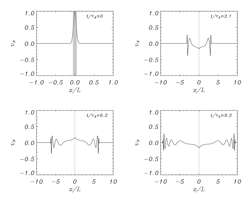
Figure 2: Plot of $v_{x}$ for different times. The initial perturbation is given by equation (13) with $w=a$ and $a=0.05L$. Note the different spatial scale for $t=0$. The grey area represents the density enhancement ($\rho_{\rm i}/\rho_{\rm e}=3$).

Figure 3: Plot of $v_{x}$ at the slab centre ($x=0$) for the numerical simulation of Figure 2. After a short transient phase the loop reaches a stationary state, oscillating at the frequency predicted by the normal mode analysis. In the inner plot the short impulsive leaky phase is displayed, showing the signal for $t/\tau_{\mathrm{A}}$ between 0 and 1.

In Figure 3 we have plotted $v_{x}$ as a function of time at the slab centre ($x=0$). The frequency of oscillation for large times is in excellent agreement with that of the fundamental kink mode calculated by solving the dispersion relation of the slab (it is basically given by eq. [1]). We also see that there is a short time interval before the loop reaches the stationary regime. In Figure 3 we have plotted a detail of this transient, which is initially dominated by the propagation of the initial disturbance inside the slab ($0\leq t/\tau_{\mathrm{A}}<2a/v_{\mathrm{Ai}}$) and is followed by the excitation of a leaky mode (for $2a/v_{\mathrm{Ai}}\leq t/\tau_{\mathrm{A}}$) because of the reflection of the disturbance at the slab boundaries. During this impulsive leaky phase the amplitude shows short period oscillations. Part of the initially deposited energy in the slab is radiated away through the fundamental kink leaky mode before the loop oscillates with the corresponding trapped mode. The period of these oscillations, which are now superimposed to the much larger period of the trapped kink mode, agrees with the period of the first leaky mode (see Terradas et al., 2005a) given by the following equation (in the limit $a/L\ll 1$)

$$P \approx \frac{2a}{v_{\mathrm{Ai}}}\frac{1}{n},\,\,\,\,\,\,\mbox{$n=1,2,...$},$$ (14)

$$\tau_{\rm d} \approx \frac{2a}{v_{\mathrm{Ai}}}\left(\ln\left|\frac{1+v_{\mathrm{Ai}}/v_{\mathrm{Ae}}}{1-v_{\mathrm{Ai}}/v_{\mathrm{Ae}}}\right|\right)^{-1}.$$ (15)

Note that the damping time ($\tau_{\rm d}=\omega_{\mathrm{I}}^{-1}$) is independent of $n$, in the limit $a/L\ll 1$ all leaky harmonics (i.e. modes with different $n$) have the same damping time. Moreover, when $v_{\mathrm{Ai}}\ll v_{\mathrm{Ae}}$ the damping time reduces to

$$\tau_{\rm d}\approx a\frac{v_{\mathrm{Ae}}}{v_{\mathrm{Ai}}^{2}}.$$ (16)

The time-signatures in the slab model are now patent, after an initial disturbance there is a short leaky transient followed by the excitation of the trapped mode, which oscillates with constant amplitude with time (in ideal MHD, i.e. without any dissipation mechanism).

It is worth noticing (see Fig. 3) that the amplitude of oscillation of the normal mode is constant but smaller than the initial amplitude ($v_{x0}$). If the perturbation is located in the external medium much less energy is trapped in the cavity. In this case the motion of the slab is dominated by the wave passing through it (described in the previous section) rather than by the eigenmode. In Figure 1 (see circles) we have plotted the evolution of the slab for a perturbation located in the corona. If we compare this result with the profile when there is no density enhancement (see continuous line) we find that the curves are almost the same. Thus, for an external excitation the slab is unable to trap a significant amount of energy. This issue is discussed later in detail for the cylindrical loop model (Section 4.2).

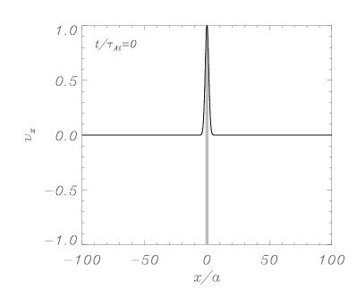
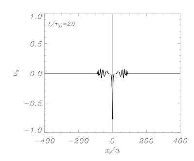
(a)                                                (b)                                              (c)                                                 (d)                                             

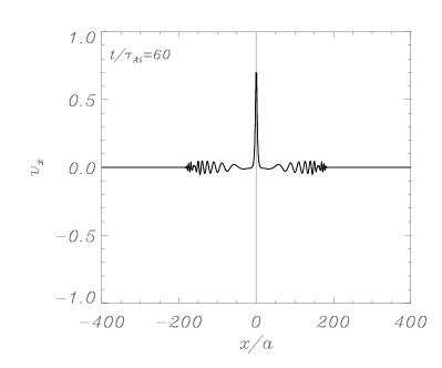
Figure 4: Plot of $v_{x}$ for different times. The initial perturbation is given by equation (13) with $w=2a$ and $a=0.02L$. In this simulation $k_{y}a=0.5$. Note the different spatial scale for $t=0$. The grey area represents the density enhancement ($\rho_{\rm i}/\rho_{\rm e}=10$).

The effect of oblique propagation ($k_{y}\neq 0$) in the slab, not included in the previous models, was investigated by Arregui et al. (2007). The properties of the eigenmodes in this system are interesting since for large $k_{y}$ the body kink mode is converted into a surface kink mode. This is clear in the time-dependent solution plotted in Figure 4 for $k_{y}a=0.5$. The system is oscillating with a trapped mode but the surface nature of the mode is revealed in Figure 4d, where we can appreciate that the amplitude of the oscillation is highly localised around the loop boundaries. Moreover, the frequency of the oscillations tends to the kink frequency (given by eq. [2]). The effect of oblique propagation has been extensively studied in the past specially in the context of resonant absorption at magnetic interfaces (see for example Lee and Roberts, 1986; Hollweg and Yang, 1988).

3.3 Multi-structures

Many loops in the solar corona are not isolated but forming groups or bundles of loops. For this reason we now consider an idealised system of two parallel loops modelled as dense plasma slabs of half-width $a$ and length $L$. The distance between the centres of the slabs is $d$. Such a configuration was studied by Luna et al. (2006). The normal mode analysis indicates that there are two kinds of normal modes (see also Díaz et al., 2005): solutions symmetric with respect to $x=0$ (both slabs move in phase) and solutions antisymmetric with respect to $x=0$ (the slabs move in anti-phase). The symmetric mode respect to the centre of the structure is the only trapped mode for all distances between the slabs while the antisymmetric mode is leaky for small slab separations. Nevertheless, there is a wide range of slab separations for which the fundamental symmetric and antisymmetric trapped modes are allowed and have very close frequencies. These modes are excited according to the parity of the initial perturbation.

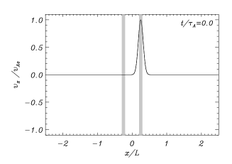
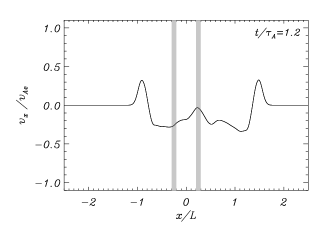
(a)                                                (b)                                              (c)                                                (d)                                             

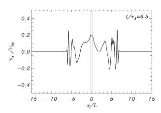
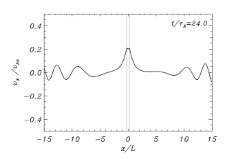
Figure 5: Time-evolution of $v_{x}$ for $d=0.5L$ and a non-symmetric initial excitation. The grey areas represent the density enhancements ($\rho_{\rm i}/\rho_{\rm e}=3$).

In Figure 5 the results of an initial excitation for a loop separation $d=0.5L$ are represented. The initial disturbance is half the sum of the symmetric and antisymmetric initial conditions. During the initial stages of the temporal evolution (Figs. 5b and c) $v_{x}$ has no definite symmetry with respect to $x=0$ because the solution is the sum of the symmetric and antisymmetric modes. These modes are the fundamental symmetric and the fundamental antisymmetric, which are, for this particular slab separation trapped and leaky, respectively. As a consequence, after some time (Fig. 5d) the antisymmetric mode amplitude is negligible in the vicinity of the slabs and the system oscillates in a symmetric manner. The oscillation is collective and different from the motion associated to the individual eigenmodes of the slabs. Rather different results are found when the system is excited with the same initial condition but for a distance between the slab centres of $d=2L$. This choice of the slab separation results in the fundamental antisymmetric mode becoming trapped. The evolution of the system is plotted for different times in Figure 6 and, although after some time the two slabs seem to move in phase (see Fig. 6b), in a later stage the right slab has transferred all its energy to the left slab and is motionless (see Fig. 6c). At an even later time (see Fig. 6d) the picture is just the opposite, with the left slab fixed and the right slab in motion, this is the result of the continuous exchange of energy. In Figure 7a we have represented $v_{x}$ at the centre of both slabs. Contrary to the behaviour in the stationary regime for symmetric or antisymmetric initial perturbations, the oscillations do not attain a constant amplitude, but they instead display a sinusoidal modulation. This is a beating phenomenon due to the simultaneous excitation of the symmetric and antisymmetric modes with similar frequencies. These frequencies are recovered from the power spectrum of the velocity at the centre of right slab (see Fig. 7b), which shows two power peaks with periods almost identical to those of the fundamental antisymmetric eigenmode and the fundamental symmetric eigenmode.

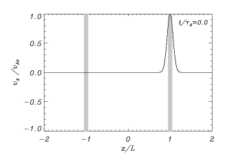
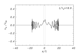
(a)                                                (b)                                              (c)                                                (d)                                             

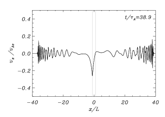
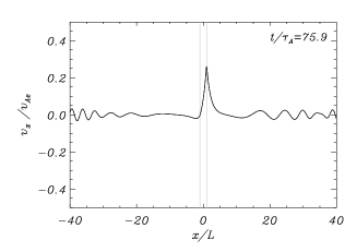
Figure 6: Time evolution of $v_{x}$ for $d=2L$ and a non-symmetric initial disturbance. Note the interchange of energy between the two slabs in the last two frames.

Figure 7: (a) $v_{x}$ measured at the centre of the slabs for the simulation shown in Figure 6. The solid and dashed lines correspond to the right and left slabs, respectively. (b) Power spectrum of the previous signal (solid line). The two vertical dashed lines indicate the periods of the fundamental antisymmetric mode and the fundamental symmetric mode calculated from the eigenvalue problem.

3.4 Curved configurations

One of the main properties of the straight slab models described before is that the system always has trapped modes. However, when the configuration is more complex then the behaviour of the solution can be leaky. For example, in two-dimensional curved configurations the Alfvén frequency changes (in general) with height, and the phase speed of the body mode might be above the local Alfvén speed at a certain position in the arcade. The character of the wave is propagating and thus the mode is leaky, being its amplitude attenuated with time due to the continuous radiation of energy.

3.4.1 Circular slab

The first time-dependent analysis of the excitation of (vertical) fast waves in a curved slab (described in Section 2.3) was done by Brady and Arber (2005). They considered a driven problem at one footpoint (and line-tying conditions at the other), and several fast body modes were excited. In Figure 8a there is an example of the excitation of a particular longitudinal harmonic. We can appreciate that the energy is not only localised around the slab (with footpoints around $x=\pm 1$), there are many fronts outside the slab that are a consequence of the leaky character of the mode. The attenuation of the oscillations with time due to the wave leakage is evident in Figure 8b. Brady et al. (2006) extended the previous model and considered in more detail the effect of wave tunnelling on the vertical fast modes. Later, the eigenmodes of the circular slab were analytically derived by Verwichte et al. (2006a, b) and Díaz et al. (2006). Verwichte et al. (2006b) showed that the calculated damping rate of fast magnetoacoustic waves is consistent with the numerical simulations of Brady and Arber (2005), so a clear link between the eigenmodes and the time-dependent solution could be established.

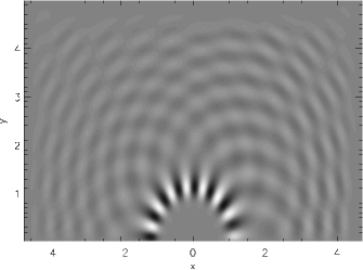
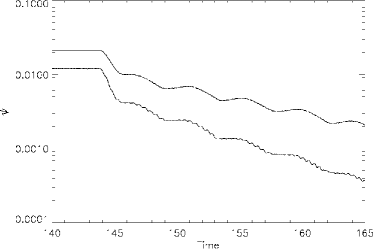
Figure 8: (a) Velocity at the end of the simulation after the driver has stopped. (b) Decay of the velocity inside the slab as a function of time due to the emission of leaky waves. The system shows three distinct phases, the stable regions due to the driver, a rapid decay phase when the driver is switched of and the stable decay of the normal model of the tube. These calculations were performed by Brady and Arber (2005).

3.4.2 Slab embedded in a coronal arcade

The main properties of propagating fast MHD waves in coronal arcades without a density enhancement have been described by Oliver et al. (1998); Terradas et al. (2008b). Recently, a battery of papers has been devoted to the analysis of the properties of these waves when a slab is embedded in the arcade. Murawski et al. (2005) showed that an impulsively disturbance near the apex of the loop is able to excite standing kink waves. Since the perturbation was very localised several standing kink modes were excited at the same time. Similar results were found by Selwa et al. (2005), who was able to excite the fundamental standing kink mode with a perturbation below the loop apex. A more detailed analysis was performed by Selwa et al. (2006) who studied how the excitation of the kink modes depends on the position of the pulse and its width. More recently Selwa et al. (2007) have extended the previous works and have shown that in the arcade leaky waves are also excited. In Figure 9a we can appreciate several wave fronts propagating upwards which are related to the emission of leaky waves (see also Fig. 8a). It should be noted that these leaky waves are slightly different from those discussed in Section 3.2. However, the short period leaky transients should be also present in the curved case, but apparently there is no clear indication of such oscillations in the previous numerical studies.

Interestingly, in all the simulations a strong damping of the vertical kink oscillations is always reported (see Fig. 9b). Although in the arcade model there is leakage due to the process described in the previous section, it is not clear that it can account for the strong damping found in the simulations. Unfortunately, up to know there are no available eigenmode calculations of a slab in the potential arcade (see Smith et al., 1997, for some preliminary attempts) which would help to clarify the origin of the damping. It is also interesting to mention that in many simulations the loop does not return to its original position, as can be appreciated in Figure 9b. This issue needs to be investigated in detail, since in the linear regime it is expected the loop to oscillate around the initial equilibrium. However, if the amplitude of the initial oscillation is large enough, the system can relax to a new magnetohydrostatic equilibrium.

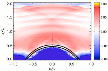
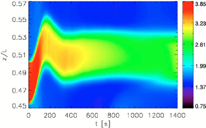
Figure 9: (a) Perturbed energy density. The position of the curved loop is marked with the black lines. (b) Density evolution at the loop apex. These results were derived by Selwa et al. (2007).

On the other hand, the influence of the dense photosphere on vertical oscillations has been analysed by Gruszecki et al. (2008). By including a dense photosphere-like layer, instead of line-tying conditions, these authors claim that in this model there is a more efficient excitation and attenuation of the vertical kink mode due to the leakage through the photosphere. Gruszecki and Murawski (2008) have analysed the effect of gravity on the oscillations and they have shown that the reported damping rate decreases as the coronal scale-height increases. However, this damping rate is still small compared with the observations. On the other hand, the effect of multi-structure in the arcade has been modelled by Gruszecki et al. (2006) by including a double stranded loop and up to five strands.

It is interesting to note that leakage in these two-dimensional structures is probably overestimated in comparison with three-dimensional loop models. In three-dimensions the eigenfunction of the kink mode is much more localised near the tube and the effect of inhomogeneities in the external medium is presumably much less important (see Terradas et al., 2006).

4 Waves in Cylinders

We turn now our attention to the analysis of kink body waves in the cylindrical loop model.

4.1 Leaky and trapped waves

The linearised MHD equations are solved in cylindrical coordinates, and since we are interested in the kink mode, we impose $m=1$ in the equations (see Terradas et al., 2007b). As in the slab model we perturb the system with an external localised disturbance with the following form

$$v_{r}(r,t=0)=v_{r0}\exp\left[{-\left(\frac{r-r_{0}}{w}\right)^{4}}\right],$$ (17)

where $r_{0}$ is the position of the centre of the disturbance and $w$ is a parameter related to its width. The results are qualitatively similar to those found in the slab configuration. The initial perturbation induces disturbances that propagate towards the loop and also wavefronts travelling in the opposite direction. Part of the energy of the initial perturbation is trapped while another part will be radiated through the excitation of the leaky modes. The radial velocity component at the centre of the loop is plotted in Figure 10a. The signal initially shows a short transient phase ($0\leq t/\tau_{\rm A}\leq 20$) which is followed by a long-period oscillation. This oscillation is due to the excitation of the trapped kink mode. Its frequency is simply the kink frequency of the tube (see dashed line in Fig. 10b). The amplitude of the oscillation of the trapped mode remains constant with time. On the other hand, the initial transitory phase is associated to the leaky modes, represented in more detail in Figure 11a. The period of the transient phase is in agreement with the period of the (fundamental) kink leaky trig mode (see dashed line in Fig. 11b). According to Cally (1986, 2003), the trig mode has the following period

$$P\approx\frac{4R}{\left(m+2n+\frac{3}{2}\right)v_{\rm Ai}},$$ (18)

$n$ being any integer consistent with $P>0$. Their damping time is

$$\tau_{\rm d}\approx R\,\frac{v_{\rm Ae}}{v_{\rm Ai}^{2}}.$$ (19)

The previous expressions are valid for $v_{\rm Ai}\ll v_{\rm Ae}$ (and for thin and long loops) and are the modifications due to the cylindrical geometry of those derived for the slab (see eqns. [14] and [16]). Again for these leaky modes the period and damping time are independent of the loop length. Additionally, in the dispersion diagram there are other families of trig leaky modes, for example, the “Type II trig modes” and the “orphan mode” (see Cally, 1986, 2003). However, these modes seem to be very difficult to excite by an initial perturbation. Something similar happens with the Principal Fundamental Leaky Mode, although it is a solution of the dispersion diagram (with a frequency very similar to that of the trapped kink mode for $k_{z}R\ll 1$) it is very difficult to excite by an initial disturbance since there is no clear evidence of such modes in the time-dependent solutions (see Terradas et al., 2007b, for a detailed investigation about the excitation of this peculiar mode). In fact, Ruderman and Roberts (2006) claim that this mode is spurious.

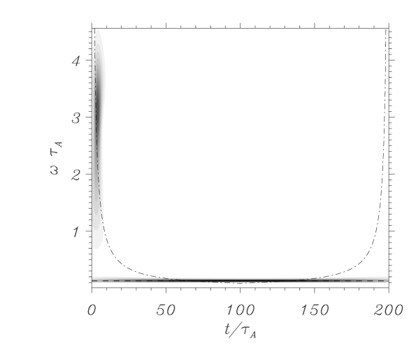
Figure 10: a) Radial velocity as a function of time at $r=0$. b) Wavelet transform of the signal. After a short transient phase, the loop oscillates with the frequency of the kink mode. The loop length is $L=30\,R$ and the density contrast is $\rho_{\rm i}/\rho_{\rm e}=3$. The initial perturbation if given by equation (17) with $r_{0}=5\,R$, $w=R$. The dashed line represents the frequency of the kink trapped mode calculated from the dispersion relation.

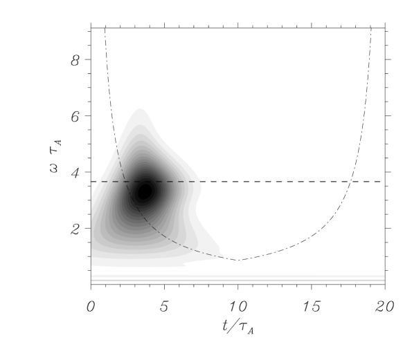
Figure 11: a) Detail of the radial velocity plotted in Figure 10 in the range $0\leq t/\tau_{\rm A}\leq 20$. b) Wavelet transform of the signal. The leaky mode is clearly identified and there is some indication of the trapped mode in the power spectrum.

4.2 Energy deposition by initial disturbances

Once we known the time signatures of the an external disturbance on the loop, we turn to the theoretical study of how the amplitude of oscillation depends on the initial disturbance. This problem has been partially addressed in the slab section, where it was suggested that an external disturbance might deposit a very small amount of energy in the loop. To analyse this problem we refer to the work of Ruderman and Roberts (2006) who solved the initial value problem using the Laplace transform to determine the motion of the tube. These authors have found that the asymptotic behaviour of the loop for $t\rightarrow\infty$ is given by the fundamental normal mode of the structure. Since we are mostly interested in the energy that is trapped in the loop and not in the transients before the loop settles in the normal mode (already discussed), instead of solving the full time-dependent problem numerically and calculating the deposited energy in the loop we use an approach based on the results of Ruderman and Roberts (2006). These authors showed that the amplitude of oscillation of the loop is basically proportional to the convolution between the initial disturbance and the eigenmode of the loop (see eqn. (7) in Terradas et al., 2007a). Using this method we can easily calculated how this amplitude (i.e. the energy of the trapped mode) depends on the different parameters. In Terradas et al. (2007a) several types of perturbations (always in the total pressure) were studied. Since we are interested on the kink modes the simplest perturbation is an $m=1$ disturbance localised in the external medium.

$$P_{0}=P_{N}\,e^{-{\left(\frac{r-r_{0}}{a}\right)}^{2}},$$ (20)

where $P_{N}$ is a normalisation constant, $r_{0}$ is the location of the Gaussian and $a$ is the width at half height (do not confuse with the loop radius $R$). This allows us to study the behaviour of the loop for different locations of the disturbance and different widths of the initial pulse. The profile of the initial perturbation for $m=1$ using the radial dependence given by equation (20) is displayed in Figure 12a. It is not a good representation of disturbance produced by for example, a flare or eruption, however its analysis is useful to understand more realistic excitations. In Figure 12b the trapped energy for the $m=1$ mode is plotted. We see that it decreases quite rapidly with $r_{0}$ while it smoothly increases with the width of the initial perturbation $a$. It is possible to find the asymptotic behaviour of the energy for $a\ll r_{0}$,

$$E\sim\frac{e^{-2|\Lambda_{e}|r_{0}}}{r_{0}^{2}}\,a.$$ (21)

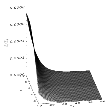
Figure 12: (a) Example of kink perturbation in the perpendicular plane to the loop axis. For this initial disturbance $r_{0}=15R$ and $a=2R$. In the vertical direction the dependence is sin($kz$). White colour corresponds to positive magnetic pressure perturbations while black colour represents negative values. The circular white region in the centre represents the loop. (b) Trapped energy as a function of $r_{0}$ and $a$ for the $m=1$ mode. For this plot $L=50R$ and $\rho_{\rm i}/\rho_{\rm e}=3$. The behaviour of the energy with $r_{0}$ and $a$ is given by equation (21) in the limit $r_{0}\gg R+a$.

Due to the strong dependence on $r_{0}$ in general only a small amount of the energy of the initial perturbation is trapped in the loop. For example, for a perturbation located at a distance similar to the loop length $r_{0}=40R$ ($L=50R$ and $a=R$), the trapped energy is $9.4\times 10^{-7}E_{0}$ ($E_{0}$ being the energy of the initial disturbance). This results clearly indicates that the loop is able to trap a very small part of the energy of the initial disturbance.

The method to calculate the energy can be easily extended to azimuthally and vertically localised perturbations. For example, we can study an azimuthally localised perturbation of the form

$$P_{0}=P_{N}\,e^{-{\left(\frac{r-r_{0}}{a}\right)}^{2}}e^{-{\left(\frac{\varphi}{\delta}\right)}^{2}}\sin(\varphi).$$ (22)

The shape of the perturbation and the energy distribution for the different $m$’s are plotted in Figure 13. The trapped energy associated with each $m$ is displayed in Figure 13b. It is clear that the energy decreases with $m$ and that the kink mode ($m=1$) has the largest energy. The energy trapped by the kink mode is between two and three orders of magnitude larger than the energy of the first fluting mode ($m=2$). Even for $m=1$ the trapped energy is quite small and, as expected, is lower than that for an excitation with a single $m$ since in that case all the initial energy was in one single mode. Qualitatively similar results are found when the width of the perturbation in the angular direction, $\delta$, is changed. Obviously, the energy of the modes in the initial perturbation is different, but again the trapped energy distribution is dominated by the kink mode.

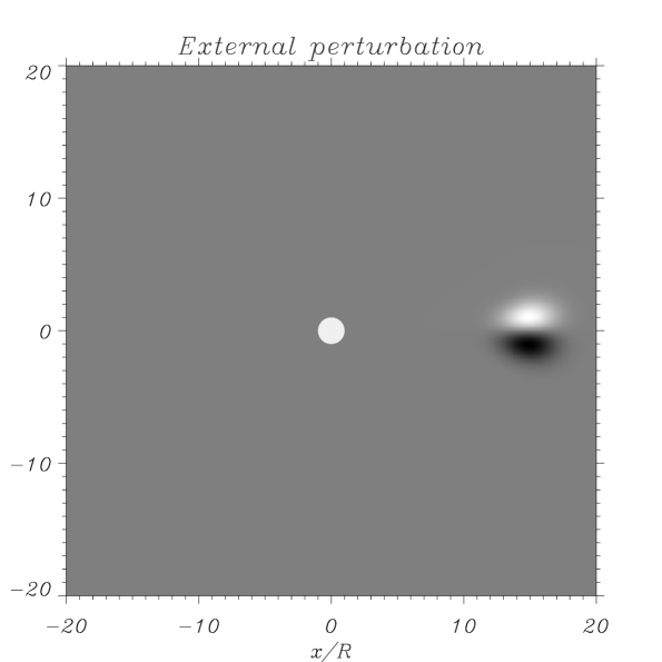
Figure 13: (a) Example of an azimuthally localised perturbation. The circular white region represents the loop. (b) Trapped energy of each eigenmode. Note that the vertical axis is in logarithmic scale. The difference in energy between consecutive modes increases with $m$. For example, the trapped energy for the $m=1$ is $4\times 10^{2}$ larger than the energy of the $m=2$. For this plot $r_{0}=40R$, $a=4R$ and $\delta=0.5$ ($L=50R$).

For a longitudinally localised perturbation we assume the following dependence

$$P_{0}=P_{N}\,e^{-{\left(\frac{r-r_{0}}{a}\right)}^{2}}e^{-{\left(\frac{z-z_{0}}{\Delta}\right)}^{2}}\sin(z\pi/L),$$ (23)

where $z_{0}$ is the longitudinal location of the Gaussian and $\Delta$ is the width of the perturbation in the longitudinal direction. The sinusoidal dependence on $z$ has been included in order to satisfy the line-tying condition. This perturbation is represented in Figure 14a and it corresponds to the case $z_{0}=L/4$, i.e. a perturbation located at a quarter of the loop length. Again the kink mode has the largest energy (see Fig. 14b). These results suggests that longitudinal harmonics are in principle more easily excited than azimuthal harmonics (which have energy differences of the order $10^{3}$).

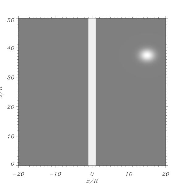
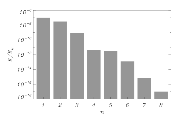
Figure 14: (a) Example of longitudinally localised perturbation. The white area represents the loop. (b) Trapped energy of each eigenmode (the vertical axis is in logarithmic scale). Note that the fundamental mode has the largest energy. For this case $r_{0}=40R$, $a=4R$ ($L=50R$), $z_{0}=L/4$ and $\Delta=L/10$.

Although there are estimations of the various types of energy released in real flares, it is not clear what amount of energy is associated with MHD waves. From the information of the previous model and the information of the coronal loop oscillations, this energy can be estimated. For example from the amplitude of the oscillating loops it is easy to estimate that they typically have an energy of $10^{19}\,\rm J$. If the perturbation is located at the loop length, then the energy of the initial disturbance should be $10^{6}$ times larger, i.e. of the order $10^{25}\,\rm J$. This quantity is, in order of magnitude, similar to the estimations of the other types of energy release. Thus, the energy of the oscillating loops can be potentially used as a seismological tool to determine the amount of energy released in real flares (related to fast MHD waves). It is interesting to note that Ballai et al. (2008) based on a model of forced oscillations (driven by EIT waves) have estimated energies of the same order of magnitude.

4.3 Role of an inhomogeneous layer at the loop boundary

The effect of a non-uniform layer on the kink oscillation has been extensively studied in the literature. The reader is referred to the review by Goossens (2008) (and references therein) about the process of resonant absorption and to its application to explain the reported damping of loop oscillations.

Figure 15: Plot of $v_{r}$ at the centre of the loop as a function of time for the numerical simulation for the initial perturbation given by equation (17). After a short leaky transient, detailed in the inner plot, the loop oscillates with the corresponding quasi-mode. The dashed line is a fit of the form $\exp(-t/\tau_{\rm d})$. In this simulation, $r_{0}=5R$, $w=2R$, $l=0.5R$, $\rho_{\rm i}/\rho_{\rm e}=3$ and $R/L=0.01$.

Here, we just want to illustrate by means of a simple time-dependent solution the process of resonant absorption that takes place at the loop boundary. For this reason, as in the homogeneous cylinder, we set up an initial disturbance given by equation (17) and we analyse the evolution of the system. Figure 15 shows the radial velocity component, $v_{r}$, at the loop centre ($r=0$) as a function of time for a loop with an inhomogeneous layer of $l=0.5R$. We can clearly identify several phases. There are initially two large extrema followed by short-period oscillations which are quickly attenuated (see inner plot of Fig. 15). After this short leaky transient the loop oscillates with a much longer period. Now the amplitude of this mode is attenuated with time (compare with Fig. 10a for the homogeneous loop, i.e. $l=0$). This damping is due to the conversion of energy from the global kink mode to the localised Alfvénic modes. By fitting an exponential function of the form $\exp(-t/\tau_{\rm d})$ to the envelope of the signal we have numerically determined the damping time, $\tau_{\rm d}$. There is quite a good agreement between the time-dependent results and the quasi-mode (which is basically the resistive eigenmode in the limit of small dissipation). The calculation of the quasi-mode provides with valuable information about the behaviour of the system, as was also shown by Ruderman and Roberts (2002) (they solved the time-dependent problem analytically using Laplace transforms).

Figure 16: Plot of $v_{r}$ (continuous line) and $v_{\theta}$ (dot-dashed line) around the resonant position for different times for the numerical simulation of Figure 15. Thin lines correspond to $R_{m}\rightarrow\infty$ and thick lines to $R_{m}=10^{5}$. Although the behaviour of $v_{\theta}$ in the inhomogeneous layer is quite different for the two values of $R_{m}$, the damping times are the same. The vertical dashed lines mark the boundaries of the inhomogeneous layer.

To show in detail the behaviour of the solutions in the inhomogeneous layer we have plotted the time evolution of the radial and the azimuthal velocity components in the range $0<r/R<2$ (Fig. 16). For $R_{m}\rightarrow\infty$ we see that small scales are generated in time in the region $R-l/2<r<R+l/2$, the amplitude of the azimuthal component being much larger than that of the radial component due to the energy conversion. The spatial scales in the inhomogeneous layer decrease due to the process of phase mixing (see for example Heyvaerts and Priest, 1983) since the local Alfvén frequency changes with position. Figure 16 also shows the time evolution for the same situation but for $R_{m}=10^{5}$ (thick lines). This is an unrealistically small value but it is illustrative since it clearly shows the effect of dissipation. Although the damping time is almost the same as for the ideal case, now the spatial scales are much larger since the short scales have been smoothed out by the effect of diffusion. However, the damping time is independent of the value of the resistivity for $R_{m}$ large. In this limit, resistivity only determines the behaviour in the inhomogeneous layer but it does not affect the conversion of energy and in consequence it does not change the damping time. It is clear that resistivity plays a secondary role and that the calculations can be done even in ideal MHD ($R_{m}\rightarrow\infty$). This property of resonant absorption is particularly attractive sine no anomalous Reynolds numbers are required to explain the damping of the oscillations.

4.4 Nonlinear effects on the kink oscillation

The previous results for the cylindrical loop were derived using the linearised MHD equations. Nevertheless, it is also interesting to study the nonlinear regime. One of the consequences of a large amplitude (nonlinear) standing kink oscillation is the generation of flows along the tube due to the ponderomotive force. This problem was studied by Terradas and Ofman (2004) in the context of coronal loops oscillations (see also Hollweg, 1971; Rankin et al., 1994). Due to the nonlinear terms, an initial disturbance produces a force imbalance along the loop which results in an up-flow from its legs. The accumulation of mass at the top of the loop (for the fundamental standing kink mode) can produce strong density enhancements, which secularly grow with time as

$$\frac{\rho_{2}}{\rho}\simeq\frac{1}{4}\left(\frac{V_{0}}{V_{A}}\right)^{2}(\omega t)^{2}\cos(2k_{z}z),$$ (24)

where $V_{0}$ is the amplitude of the initial disturbance. However, if the plasma beta is different from zero the gas pressure gradient becomes dominant and inhibits the concentration of mass. The density enhancements are then of the form

$$\frac{\rho_{2}}{\rho}\simeq\frac{1}{2}\left(\frac{V_{0}}{V_{A}}\right)^{2}\left(\frac{\omega}{\omega_{s}}\right)^{2}[1-\cos(\omega_{s}t)]\cos(2k_{z}z),$$ (25)

where $\omega_{s}=2k_{z}\,c_{s}$, being $c_{s}$ the sound speed. This expression can be potentially used as an indirect way to determine the sound speed in the solar corona if such enhancements are reported in the observations (see Terradas and Ofman, 2004, for an example). Thus, although the zero-$\beta$ approximation is in general justified under coronal conditions, the role of the gas pressure is important in nonlinear studies of standing kink oscillations (and also in propagating kink body modes) since it avoids the eventual destruction of the tube due to the ponderomotive force.

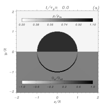
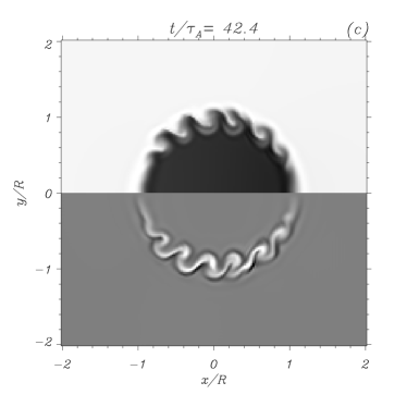
Figure 17: The top half of each panel displays the density (symmetric respect to $y=0$) and the bottom half the vorticity (antisymmetric respect to $y=0$) at $z=L/2$ (half the loop length) for different times. In this simulation the following parameters have been used: $L=10R$, $\rho_{\rm i}/\rho_{\rm e}$=3, $v_{0}=0.1v_{\rm Ai}$, and a full domain of $[-6R,-6R]\times[-6R,6R]\times[0,10R]$. The kink oscillation develops a Kelvin-Helmholtz instability at the loop boundary.

On the other hand, nonlinearity can significantly change the motion of the plasma fluid at certain locations in the tube. It is important to remark that the kink oscillation of a cylindrical loop with a sharp or smooth transition involves strong shear motions at the tube boundary (see for example Fig. 16). Such motions might be liable to develop a Kelvin-Helmholtz instability. The most likely place for the KHI to occur is where the velocity is largest and the magnetic field is perpendicular to the velocity (see for example Rankin et al., 1993). For the fundamental standing kink mode this is precisely the antinode of the velocity, located at half the loop length from the photosphere. In order to understand this problem we show the results of solving the full nonlinear MHD equations in three-dimensions (see Terradas et al., 2008a). This is the extension of the linear problem studied in Sections 4.1 and 4.3. Now the initial perturbation is located inside the tube. The evolution of the density (for a sharp transition model) and the longitudinal component of the vorticity of a representative case in a weak nonlinear regime is shown in Figure 17 at different time intervals. The initial perturbation produces a lateral displacement of the tube in the $x-$direction. As in the linear regime the tube starts to oscillate around the initial position, but small length scales quickly develop at the boundary (see Fig. 17b). These small scale structures grow with time (see Fig. 17c) and several rolls form at the loop edge. Around $x=\pm R$ and $y=0$ the density is almost undisturbed because there are no shear motions at this position. At later stages of the evolution (Fig. 17d) the small spatial scales are still localised at the boundary. As a result of the instability the shape of the tube at the boundary has been considerably changed.

On the other hand, if instead of a sharp transition a thick inhomogeneous layer between the tube and the environment is included then the motions are characterised by strong phase-mixed scales (see Fig. 16 for the linear results). In this situation the instability is still present, but it develops more slowly than in the sharp transition case. This is due to the fact that the thicker the layer the later the generation of small length scales due to phase mixing, and thus the eventual onset of the instability. This process seems to be related to the development of the KHI for torsional Alfvén waves described by Browning and Priest (1984). Interestingly, for thick layers the attenuation of the central part of the tube due to resonant absorption (i.e. the damping rate) is not significantly altered by the changes at the boundary due to the shear instability.

Finally, it must be noted that up to now, there is no evidence of such instability from the observation of oscillating loops. It is known that magnetic twist, not included in the model, might decrease or even suppress the instability since the presence of a magnetic field component along the flow stabilises the KHI. Nevertheless, a tube with very large azimuthal magnetic field is subject to the instabilities of the linear pinch. Therefore, the azimuthal component of the magnetic field of a stable flux tube in the solar corona is probably constrained to be in a specific range. The absence of observational evidences of the instability might be also due to a lack of spatial resolution of the telescopes. This issue about this instability is very promising and needs to be investigated in more detail in the future from both the theoretical (including twist in the tube models) and the observational point of view.

4.5 Multi-structure

Now we leave the single tube model to study the collective motion of several tubes again in the linear regime. We start with two parallel homogeneous straight cylinders of radius $R$, length $L$, and separation between centres $d$. This is the equivalent to the slab configuration analysed in Section 3.3. In this two-tube problem Luna et al. (2008) showed that there are four collective fundamental kink-like trapped modes (see also van Doorsselaere et al., 2008). The velocity field is more or less uniform in the interior of the loops, and so they move basically as a solid body, while the external velocity field has a more complex structure. The four velocity field solutions have a well defined symmetry with respect to the $y$-axis. The symmetric mode has the velocity field inside the tubes lying in the $x$-direction and is symmetric with respect to the $y$-axis. This is the $S_{x}$ mode, where $S$ refers to the symmetry of the velocity field and the subscript $x$ refers to the direction of the velocity inside the tube. The same nomenclature is used for the other modes. The following mode has the velocity inside the cylinders mainly in the $x$-direction and it is antisymmetric with respect to the $y$-axis, we call this mode $A_{x}$. Similarly, we have the modes $S_{y}$ and $A_{y}$. The pressure field of the $A_{x}$ and $S_{y}$ modes is symmetric with respect to the $y$-axis, while that of the $S_{x}$ and $A_{y}$ modes is antisymmetric.

In Figure 18, the time evolution is shown for a pulse in the $v_{x}$ component initially centred on the right loop (see Fig. 18a). In Figure 18b, the pulse reaches the left tube and passes through it, the system still being in the transient phase. In Figures 18c and 18d the system oscillates in the stationary phase. The oscillatory amplitude in the left loop grows with time in the stationary phase, while the amplitude in the right loop decreases in the time interval shown in Figures 18c and 18d. The left tube begins its motion through the interaction with the right loop, i.e. by a transfer of energy from the right loop to the left loop. This process is reversed and repeated periodically: once the left loop has gained most of the energy retained by the system, so that the right loop is almost at rest, the left tube starts giving away its energy to the right cylinder, and so on. We find again the beating phenomenon (see Section 3.3), since the initial disturbance excites the $S_{x}$ and $A_{x}$ modes with the same amplitude.

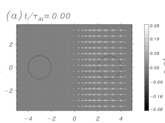
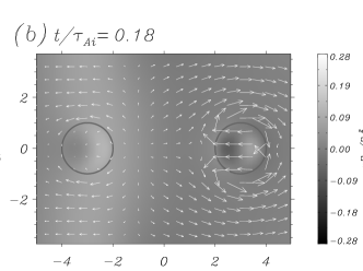
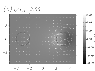
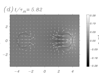
Figure 18: Time-evolution of the velocity field (arrows) and total pressure field ( contours), for a separation between loops $d=6R$ (in this model $a=R$). The two circles mark the positions of the loops at $t=0$. The panels show different evolution times. In (a) the initial condition over the velocity field is represented. In panel (b) the tubes are in the transient phase. In panels (c) and (d) the system oscillates in the stationary phase with a superposition of the $S_{x}$ and $A_{x}$ normal modes.

The extension of the previous model to multi-stranded configuration but with nonuniform layers has been carried out by Terradas et al. (2008c). In this work a smooth density transitions between the tubes is allowed. In Figure 19a the two-dimensional distribution of the density (the cross section of the composite loop) is plotted for a particular configuration. The loop density has an inhomogeneous distribution with quite an irregular cross section and boundary. In this so-called “spaghetti model” the distance between the strands is quite small and a strong dynamical interaction between them takes place. When an initial perturbation is launched in the system the structure basically oscillates in the direction of the perturbation. This kink-like motion of the bundle of loop results in a strong mode conversion at the inhomogeneous layers. We can see the shear motions due to the resonant coupling in Figure 19b (see the phase-mixed scales at the boundary). As in the cylindrical model described in Section 4.3 the energy of the kink-like mode is transferred to the layer, this is clear from the energy distribution at a particular given time displayed in Figure 20a. In Figure 20b the averages of the velocity in three different regions (marked with the labels $a$, $b$ and $c$) are represented. We see that the signals are almost the same, they have the same dominant period and the same damping time. This is due to the global nature of the motion, and the attenuation with time is the consequence of the energy conversion due to resonant absorption (this result is completely equivalent to that found in the single cylindrical inhomogeneous loop model, see Fig. 15). These results clearly demonstrate that the mode conversion takes place in quite irregular geometries. Regular magnetic surfaces are not necessary for this mechanism to work efficiently as was already anticipated by Ruderman (2003) using an elliptical cross section loop model. This indicates that resonant absorption is quite a robust damping mechanism and although we have analysed a particular system, the behaviour found in the present equilibrium is expected to be quite generic of inhomogeneous plasma configurations. The resonant coupling between fast and Alfvén modes can hardly be avoided in a real situation since inhomogeneity is certainly present in coronal loops, for these reasons, resonant absorption seems to be quite a natural damping mechanism.

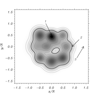
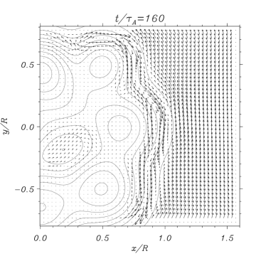
Figure 19: (a) Cross section of the density of the multi-stranded loop model. The contour lines represent curves of constant Alfvén frequency, (they also represent contours of constant density). The thick line corresponds to the Alfvén frequency that matches the frequency of the global mode. (b) Detail of the velocity field at $t=160\,\tau_{\rm A}$.

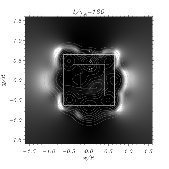
Figure 20: (a) Energy distribution at a given instant (when most of the energy has been transferred to the inhomogeneous layers). The three square boxes labelled with $a$, $b$, and $c$ mark the regions where the velocity averages have been computed to determine the damping time. (b) Time evolution of the spatially averaged $v_{y}$ component as a function of time. The continuous, dot-dashed, and dotted lines correspond to the (normalised) averages in the square regions marked with labels $a$, $b$, and $c$ in (a), respectively. The profile of the three signals is almost the same since the loop is oscillating with a global mode. The damping per period in this configuration is $\tau_{\rm d}/P=2.3$.

4.6 Curved configurations

A curved cylindrical model involves a three-dimensional model. Kink oscillations in three-dimensional configurations are discussed in this volume by L. Ofman, so the reader is referred to this review and references therein. Here we just want to comment a few points about these works. One of the striking findings of the three-dimensional studies is that, as in some two-dimensional works, the damping rate found in the simulations is much stronger that the reported by the observations. This damping is usually attributed to the wave leakage due to curvature. However, up to now there are no comprehensive numerical studies about this process in 3D. Moreover, if there is leakage in three-dimensions, because the frequency of the kink mode is above the local Alfvén frequency, then it is unavoidable to have an external resonance (basically where the frequency of the kink mode is equal to the local Alfvén frequency). This external resonance (see Terradas et al., 2006) will also contribute to the attenuation of the kink oscillation due to resonant absorption. The implications of this mechanism have not been yet addressed in three-dimensional studies.

5 Conclusions and Discussion

We have described the main efforts that have been done so far to understand standing kink oscillations in coronal loops. We have reviewed the time-dependent studies in simple slabs and cylindrical loop models. The effect of curvature and inhomogeneity has been also described in some detail, and preliminary studies about the possible effects of nonlinearity have been explained. However, the time-dependent modelling of kink oscillations is still in a primitive stage and there are several issues that need to be addressed, being the attenuation of the oscillations one of the most interesting.

In particular, the analysis of the damping by wave leakage in two and three-dimensional models needs to be investigated in detail, this might help to provide clues about the problem of the strong damping found in most of the numerical simulations. Nevertheless, here it is worth to draw the attention about the overlooked problem of numerical dissipation. Very often, in many numerical studies the effect on the results of the intrinsic numerical viscosity of the numerical scheme is not studied or quantified. Moreover, in some numerical studies dissipation is explicitly added to stabilise the code. The issue of the dissipation is very relevant, specially if we want to extract quantitative information about the damping rates with the goal of identifying the possible damping mechanism that produce the attenuation. Too much artificial dissipation can simple mask the physics behind the damped oscillations and lead to the wrong interpretation of the results.

Another remark about the numerical simulations is that in general in most of the works the full set of nonlinear MHD equations are numerically solved. Nevertheless, in the majority of the published papers about kink oscillations, the linear regime is considered (the amplitude of the waves are very small in comparison with the local Alfvén or sound speed). Before any problem is attempted to be studied we should first ask whether it is worth to solve the full nonlinear equations instead of the simple linearised system of equations. One of the advantages of the linear regime is that (for simple equilibrium configurations) we can make Fourier analysis in some direction to simplify the problem (since that direction is incorporated in the equations through a certain wavenumber). This is not possible when the full nonlinear MHD equations are solved. Obviously, if we are interested in nonlinear processes, such as shocks or some types of instabilities then it is required to solve the nonlinear MHD equations.

Finally, we would like to point out that in other branches of sciences, for example in computational fluid dynamics, it is a standard practice to attempt to repeat experiments soon after they are published. This is a necessary aspect of the scientific method and it can viewed as an excellent learning tool. We think that it might be interesting to apply the idea of reproducible research (see the paper about this topic of LeVeque, 2006) in numerical MHD. This would mean to make available the codes used to create the figures and tables in a paper in such a way that the reader can download the codes and run them to reproduce the results shown in the paper.