No Evidence of Time Dilation in Gamma-Ray Burst Data

Abstract

Gamma-Ray Bursts have been observed out to very high redshifts and provide time measures that are directly related to intrinsic time scales of the burst. Einstein’s theory of relativity is quite definite that if the universe is expanding then the observed duration of these measures will increase with redshift. Thus gamma-ray burst measures should show a time dilation proportional to redshift. An analysis of gamma-ray burst data shows that the hypothesis of time dilation is rejected with a probability of 4.4$\times 10^{-6}$ for redshifts out to z=6.6. Traditionally the lack of an apparent time dilation has been explained by an inverse correlation between luminosity and time measures together with strong luminosity selection as a function of redshift. It is shown that the inverse correlation between luminosity and some time measures is confirmed, but using concordance cosmology strong luminosity selection cannot be achieved. It may be possible to explain the apparent lack of time dilation with a combination of gamma-ray burst selection, some luminosity evolution and some time measure evolution. But this requires a remarkable coincidence in order to produce the apparent lack of time dilation. However the data are consistent with a static cosmology in a non-expanding universe.

keywords(cosmology: observations, large-scale structure of universe, theory, gamma rays: bursts)

1 Introduction

Gamma-Ray bursts (GRB) are transient events with time scales of the order of seconds and with energies in the X-ray or gamma-ray region. Piran04 provides (a mainly theoretical) review and Bloom03 give a review of observations and analysis. Although the reviews by Meszaros06 and Zhang07 cover more recent research and provide extensive references they are mainly concerned with GRB models. The only other objects for which time dilation has been observed are type 1a supernovae (Goldhaber01; Foley05). However this time dilation claim has been questioned by (Crawford06; Crawford09a; Crawford09b). Although the supernovae observations are clearly important in choosing between cosmologies they are not relevant to whether GRB show the effects of time dilation. This paper considers only the direct GRB observations and makes no assumptions about GRB models.

The search for the time dilation signature in data from GRB has a long history and before redshifts were available Norris94; Fenimore95a; Davis94 claimed evidence for the time dilation effect by comparing dim and bright bursts. However Mitrofanov96 found no evidence for time dilation. Lee00 found rather inconclusive results from a comparison between brightness measures and timescale measures. They also provide a brief summary of earlier results. Once redshifts became available Chang01 and Chang02 using a Fourier energy spectrum method and Borgonovo04 using an autocorrelation method claim evidence of time dilation. The standard understanding, starting with Norris02 and Bloom03, is that time dilation is present but because of an inverse relationship between luminosity and time measures it cannot be seen in the raw data. Because a strong luminosity-dependent selection produces an average luminosity that increases with redshift there will be a simultaneous selection for time measures that decrease with redshift which can cancel the effects of time dilation.

Here it is argued that there is no evidence for strong luminosity selection. Alternately the strong luminosity-redshift dependence may be due to luminosity evolution. In this case there is an increase in the average luminosity with redshift and not a selection of more luminous GRB. Consequently those time measures that show a strong relationship with luminosity must have evolved in a similar manner. Although it is possible that a combination of luminosity selection, selection of GRB by other characteristics and evolution may be sufficient to cancel time dilation it does require a fortuitous coincidence of these effects to completely cancel time dilation in the raw data. Another explanation is that the universe is not expanding and thus there is no time dilation. Not only is it shown that the data are consistent with a static cosmology but it is also shown that if a static cosmology is valid, it can readily explain the results from a concordance cosmology analysis.

The structure of this paper is to analyse recent GRB data to verify that there is no indication of time dilation in the raw time measures. Since the necessity of having an observed redshift makes this a specially selected sample of GRB the next step is to confirm that it shows the well known inverse relationship between luminosity and some time measures. It is also found, in agreement with the suggestion by (Frail01; Bloom03), that the data are consistent with the average energy of the GRB being constant. Since the dependence of the luminosity on redshift is strong it is necessary to see whether it is due to selection or evolution. The next step is to investigate the selection process where it is shown that the data are inconsistent with strong luminosity-selection as a function of redshift. Then the alternative of luminosity evolution is considered. Next direct selection that depends on other characteristics of the GRB that could partially cancel the time dilation is considered. Although none of them is individually sufficient there is a possibility that a combination could be sufficient. Finally the data are shown to be in agreement with a static cosmology.

Recently Schaefer07a has provided an excellent analysis of GRB relationships and provides tables of burst parameters of 69 bursts observed with redshift parameter z varying from 0.17 to 6.6. This redshift range is greater than that for type 1a supernovae for which there is also intrinsic timing information. Of relevance here are $\tau_{lag}$ the lag time between a band of high energy gamma-rays and a band of lower energy gamma-rays, and $\tau_{RT}$ the shortest time over which the GRB light curve rises by half the peak flux of the pulse. A further measure is $V$, which is a measure of the variability of the light curve. Crudely, it is the number of spikes per second. In practice it is a normalised estimate of the fluctuations in the light curve relative to a smoothed version of the light curve. Finally Gehrels07 provides estimates of the time span $T_{90}$ that contains 90% of the counts. These four time measures are determined from the original gamma-ray observations and are independent of any model for the burst mechanism. It can be argued that since the physical processes that produce these time measures are not well understood we cannot use them to test for time dilation. However time dilation must apply to all time measures. Here we start with the simplest assumption is that the characteristics of the GRB are the same at all redshifts. Then we consider whether evolution can explain the results.

In an expanding universe, the raw time measures should show an average duration that is directly proportional to ($1+z$), and the variability should show an inverse relationship. Time dilation provides a much stronger test of universal expansion than the Hubble redshift of frequencies. Of many explanations for the Hubble frequency redshift, the only one that includes time dilation is universal expansion.

This analysis uses the current standard cosmology, concordance cosmology, and following Schaefer07a the mass density $\Omega_{M}$ is taken to be 0.27 and $\Omega_{\Lambda}$ which is proportional to the cosmological constant, has a value of 0.73. In this work the Hubble constant $H_{0}$ is assumed to have the value of 70 km s${}^{-1}$ Mpc${}^{-1}$. Because of the relatively small numbers the arguments used here are often statistical and the paper starts with a brief description of how the uncertainties are treated. Since the expected effect of time dilation is that it is a linear function of ($1+z$) it is appropriate to determine the exponent of ($1+z$) that has the best fit to the data and see if it is compatible with unity.

2 Uncertainties

Since the observations have a very large spread, it is desirable to use logarithms so that the dynamic range is reduced, scale factors are irrelevant and the influence of outliers is reduced. In addition many of the variations in GRB such as external pressure and chemical composition are multiplicative. Thus from the central limit theorem the logarithm of a variable is likely to be closer to a normal distribution that the variable itself.

Although the measurements provided by Schaefer07a have measurement uncertainties, it is very obvious, as Schaefer07a has noted, that their scatter is much greater than the uncertainties would suggest and this scatter is mainly due the intrinsically different properties of the individual GRB. Therefore it is most likely that measurement uncertainties are a poor guide to the accuracy of each observation, and thus it is inappropriate to assume that the overall uncertainty is proportional to the measurement uncertainties. Instead a simple model is adopted where the additional uncertainty due to the intrinsic scatter is made proportional to the actual measure. Thus the variance for a measurement $y_{i}$ is set equal to $\sigma_{i}^{2}$+$(\eta y_{i})^{2}$ where $\sigma_{i}$ is the measurement uncertainty for that measurement, $y_{i}$ is its value and $\eta$ is a constant for all the $y_{i}$ measures. The values of $\eta$ are estimated by requiring that the residual $\chi^{2}$ after doing a linear regression of $\log(y)$ against $\log(1+z)$ is equal to the number of degrees of freedom. This regression is done in order to remove any cosmologically important systematic effects on the estimate of $\eta$. Because this new term dominates the variance this procedure is almost the same as using unweighted values in regressions with $\log(y)$.

When both inputs to a linear regression have significant uncertainties the method ($fitexy$ subroutine) promoted by Press07 is used. This method retains symmetry between the variables in that the results are independent of which variable is chosen as the independent variable. For a linear regression where the $y_{i}$ variable has an uncertainty $\sigma_{i}$ and the $x_{i}$ variable has an uncertainty $\epsilon_{i}$ the method minimises $\chi^{2}$ where

$$\chi^{2}=\sum\limits\frac{(y_{i}-a-b\>x_{i})^{2}}{\sigma^{2}_{i}+(b\epsilon_{i})^{2}}$$

If the uncertainties in $x$ are small enough this method reduces to the standard weighted regression. Finally a small adjustment is made to the estimated errors in the regression results to make the residual $\chi^{2}$ value equal to the number of residual degrees of freedom. In effect the uncertainties in the measurements are used only to determine the relative weights. The final scaling of the uncertainty in any derived result is determined by the residual $\chi^{2}$. Since in this case this procedure increases the magnitude of the uncertainties the result is to decrease the significance of any dependency between the data and time dilation. It has been argued that the intrinsic scatter of the time variables is too large to show a significant dependence on time dilation. If this is true and time dilation is present then there is no change in the value of the expected exponent but the uncertainty in the exponent will be large.

3 Procedure and results

Since there appears to be a clear distinction between short GRB, with $T_{90}$ less than 2 seconds (Piran04; Borgonovo04), and long GRB, the analysis is restricted to long GRB. Data for $\tau_{lag}$, $V$, and $\tau_{RT}$ are taken from Schaefer07a (his Table 4) and $T_{90}$ data come from Gehrels07. This second data set provided an extra 39 GRB that had only $T_{90}$ measurements. There were two measurements that were rejected as being outliers at the $5\sigma$ level. These outliers were $\tau_{lag}$ from GRB030528, and $\tau_{RT}$ from GRB050824. In addition GRB020903 with a redshift of 0.25 was rejected because it was extremely weak and had no time measures. Since GRB60116 has a photometric redshift and Tanvir06 note that it is close to the Orion Nebula where the extinction is unreliable it has been omitted.

The estimation method is to use weighted linear regression, using the logarithms of the raw variables, to estimate the exponent as slope of the regression. Most of the regressions have $\log(1+z)$ as the independent variable. The estimates of the exponent for each of the four raw (i.e, uncorrected for time dilation) time measurements are shown in Table LABEL:grb1 together with the number of observations, the uncertainty (all uncertainties quoted are one-sigma values) in the exponent and the probability $p$ that the data are consistent with time dilation. The probability assumes a normal distribution for the exponents and is the probability that the observed exponent is greater than unity (or less than -1 for $V$). In order to improve accuracy all four time measures were combined (as logarithms) into a new variable $\tau_{4}$ which is the weighted mean of the logarithms of $T_{90}$, $\tau_{lag}$, $1/V$, and $\tau_{RT}$. The weights (3.80, 2.63, 11.63, and 3.93 respectively) were the reciprocals of the average variances of their logarithms. To help avoid bias only bursts which had at least three measures were used to compute $\tau_{4}$. Although $\tau_{4}$ has no physical significance its use in this context is legitimate because the time dilation must apply to all the time measures. Figure 1 shows a plot of $\tau_{4}$ as a function of redshift where the dashed line is the line of best fit. The solid line shows the expected value with time dilation which is a power law with an exponent of unity. The $\chi^{2}$ value for an exponent of zero is 44.24 (46 DoF) and for an exponent of unity it is 63.69 (46 DoF). Butler07 have done a different reduction of 218 Swift bursts of which 77 events have measured redshifts. Using only bursts with $T_{90}$ less than 2 seconds this data has an exponent for $T_{90}$ as a function of $(1+z)$ of $0.28\pm 0.31$ in excellent agreement with the value in Table 1. The advantage of this data is that it is a homogeneous set derived from one satellite.

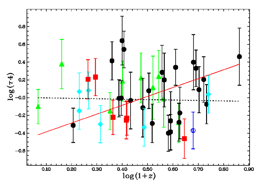
Figure 1: Plot of the raw combined time measure $\tau_{4}$ as a function of redshift. The dotted line is the line of best fit with a slope of -0.05$\pm$0.23. The solid line (in red) is the expected line for time dilation with a slope of one. The legend in Figure LABEL:g2 shows the symbol and colour for each satellite detector which discovered that GRB. This legend is the same for all figures.

It is clear both from Figure 1 and Table LABEL:grb1 that $\tau_{4}$ shows no dependence on redshift and that with an exponent of -0.04$\pm$0.23 there is a probability (one sided normal distribution) of 4.4$\times 10^{-6}$ that the exponent is greater than or equal to unity. Although the central limit theorem predicts that the distribution of exponents should approximate the normal distribution it is in the tails of the distribution that we might expect some discrepancy. Thus the estimate 4.4$\times 10^{-6}$, for the probability could be slightly incorrect which does not alter the conclusion that the probability that the raw time measures are consistent with time dilation is extremely unlikely. In addition all the results are fully consistent with an exponent of zero. However it should be noted that $\tau_{lag}$ has a 9% probability of being consistent with time dilation.

Table 1: Analysis of gamma-ray bursts for time dilation

Variable	$\eta$${}^{a}$	N${}^{b}$	Exponent${}^{c}$	Probability${}^{d}$
$T_{90}$	0.51	84	0.28$\pm$0.28	4.7$\times 10^{-3}$
$\tau_{lag}$	0.55	36	0.18$\pm$0.61	8.9$\times 10^{-2}$
$V$	0.25	49	-0.18$\pm$0.23	2.5$\times 10^{-7}$
$\tau_{RT}$	0.48	58	0.01$\pm$0.37	2.9$\times 10^{-3}$
$\tau_{4}$	-	46	0.03$\pm$0.12	4.4$\times 10^{-6}$

${}^{a}$The value of $\eta$ for the logarithm of this variable.
${}^{b}$The number of GRB used.
${}^{c}$The exponent with respect to ($1+z$).
${}^{d}$The probability of the exponent being greater than one (less than minus one for $V$).