A Quintet of Black Hole Mass Determinations

Abstract

We report five new measurements of central black hole masses based on STIS and WFPC2 observations with the Hubble Space Telescope and on axisymmetric, three-integral, Schwarzschild orbit-library kinematic models. We selected a sample of galaxies within a narrow range in velocity dispersion that cover a range of galaxy parameters (including Hubble type and core/power-law surface density profile) where we expected to be able to resolve the galaxy’s sphere of influence based on the predicted value of the black hole mass from the $M$–$\sigma$ relation. We find masses for the following galaxies: NGC 3585, $M_{\mathrm{BH}}=3.4^{+1.5}_{-0.6}\times 10^{8}~{}{\mathrm{M}}_{\scriptscriptstyle\odot}$; NGC 3607, $M_{\mathrm{BH}}=1.2^{+0.4}_{-0.4}\times 10^{8}~{}{\mathrm{M}}_{\scriptscriptstyle\odot}$; NGC 4026, $M_{\mathrm{BH}}=2.1^{+0.7}_{-0.4}\times 10^{8}~{}{\mathrm{M}}_{\scriptscriptstyle\odot}$; and NGC 5576, $M_{\mathrm{BH}}=1.8^{+0.3}_{-0.4}\times 10^{8}~{}{\mathrm{M}}_{\scriptscriptstyle\odot}$, all significantly excluding $M_{\mathrm{BH}}=0$. For NGC 3945, $M_{\mathrm{BH}}=9^{+17}_{-21}\times 10^{6}~{}{\mathrm{M}}_{\scriptscriptstyle\odot}$, which is significantly below predictions from $M$–$\sigma$ and $M$–$L$ relations and consistent with $M_{\mathrm{BH}}=0$, though the presence of a double bar in this galaxy may present problems for our axisymmetric code.

1. Introduction to Black Hole Mass Measurements

This paper is the latest in a campaign to model the central regions of galaxies to determine masses of putative black holes from images and spectra taken with the Hubble Space Telescope (HST). The discovery of the presence of a massive dark object (probably a black hole) in almost all galaxies having bulges, and the scaling relations found versus host-galaxy properties, will stand as one of the important legacies of this great observatory.

Masses were first determined from stellar velocity measurements made with ground-based telescopes having the best possible spatial resolution, together with isotropic kinematic models (Dressler & Richstone, 1988). When combined with the spatial resolution of HST, this method has become the standard for black hole mass measurements (e.g., van der Marel et al., 1998; Gebhardt et al., 2000b). Black hole masses have also been derived from stellar proper motions in our Galaxy (Genzel et al., 2000; Ghez et al., 2005), from megamaser measurements of gas disks around central black holes (e.g., Miyoshi et al., 1995), and from gas velocity measurements (e.g., Barth et al., 2001). Reverberation mapping has also been used to find virial products in variable active galactic nuclei (AGNs; e.g., Peterson et al., 2004).

Direct dynamical masses are the foundation for all scaling relations used to infer black hole masses in active galaxies; all measures of black hole mass are derived from the direct, dynamical measurements. Indirect mass indicators, such as AGN line widths, are calibrated to reverberation mapping measurements (Bentz et al., 2006), which are themselves normalized against the direct dynamical measurements (Onken et al., 2004).

A central goal of a companion paper (Gültekin et al., 2009) is the accurate measurement of the intrinsic or cosmic scatter in the $M$–$\sigma$ and $M$-$L$ relationships (Magorrian et al., 1998; Gebhardt et al., 2000a). We have thus chosen to augment the existing sample of $M_{\mathrm{BH}}$ measurements with new determinations of $M_{\mathrm{BH}}$ for five galaxies selected to fall within a narrow range in velocity dispersion. Along with results from the literature, this provides a number of galaxies in a narrow range in velocity dispersion large enough that we may probe the intrinsic scatter in the relation without biases incurred by, for example, looking only at residuals to power-law fits.

We present observations of the centers of five early-type galaxies in § 2, including HST observations in § 2.3, ground-based imaging in § 2.4, and ground-based spectra in § 2.5. We report results of dynamical models and black hole masses in § 3, and summarize in § 4. In the Appendix, we provide our data tables.

2. Observations for New $M_{\mathrm{BH}}$ Determinations

2.1. Observational Sample

The five galaxies in this study were selected to come from a narrow range in velocity dispersion ($180<\sigma<200~{}\mathrm{km~{}s^{-1}}$) based on HyperLEDA central velocity dispersion measures (Paturel et al., 2003). We chose this range because (1) it includes galaxies with $M_{B}\approx-20$ mag where both core and power-law surface-brightness profiles exist and (2) it includes both late- and early-type galaxies. We selected galaxies with distances such that the predicted radius of influence was larger than 0$\farcs$1. The radius of influence is defined as

$$R_{\mathrm{infl}}\equiv\frac{GM_{\mathrm{BH}}}{\sigma^{2}\left(R_{\mathrm{infl}}\right)},$$ (1)

where the velocity dispersion $\sigma$ is evaluated at the radius of influence. This obviously requires an iterative solution, but it converges quickly. The predicted mass comes from the central velocity dispersion measurement and the $M$–$\sigma$ fit of Tremaine et al. (2002).

The sample of new galaxies and their properties are presented in Table 1. Distances are calculated assuming a Hubble constant of $H_{0}=70~{}~{}\mathrm{km~{}s^{-1}}~{}\mathrm{Mpc^{-1}}$. We also provide “Nuker Law” surface-brightness profile parameters as a function of radius given by

$$I\left(r\right)=2^{\left(\beta-\gamma\right)/\alpha}I_{b}\left(\frac{r_{b}}{r}\right)^{\gamma}\left[1+\left(\frac{r}{r_{b}}\right)^{\alpha}\right]^{\left(\gamma-\beta\right)/\alpha},$$ (2)

which is a broken power-law profile (Lauer et al., 1995). In addition to the five galaxies whose black hole masses are reported in this paper, we observed five others with HST as part of the same observing proposal. Two of these (NGC 1374 and NGC 7213) had very low signal-to-noise ratio (S/N). The remaining three (NGC 2434, NGC 4382, and NGC 7727) will be presented in a future paper.

Table 1Observational Sample

Galaxy	Type	Distance	$M_{V}$	Profile	$r_{b}$	$I_{b}$	$\alpha$	$\beta$	$\gamma$
N3585	S0	21.2 $\pm$ 1.8	$-22.01$	$\wedge$	37.0	14.72	1.62	1.06	0.31
N3607	E	19.9 $\pm$ 1.6	$-21.56$	$\cap$	70.3	16.87	2.06	1.70	0.26
N3945	SB0	19.9 $\pm$ 3.0	$-21.14$	$\backslash$	3.9	18.62	0.30	2.56	-0.06
N4026	S0	15.6 $\pm$ 2.0	$-20.32$	$\backslash$	3.0	15.23	0.39	1.78	0.15
N5576	E	27.1 $\pm$ 1.7	$-21.67$	$\cap$	549.2	17.81	0.43	2.73	0.01

Note. — Distances are given in Mpc assuming a Hubble constant of $H_{0}=70~{}~{}\mathrm{km~{}s^{-1}}~{}\mathrm{Mpc^{-1}}$. All distances come from surface brightness fluctuations by Tonry et al. (2001) except for NGC 3945, which comes from group distance by Faber et al. (1989). The uncertainties to distances include random errors only. The third column gives $V$-band absolute magnitudes taken from Lauer et al. (2005) and may be converted to $V$-band luminosities via $\log(L_{V}/{\mathrm{L}}_{\scriptscriptstyle\odot,V})=0.4(4.83-M_{V})$ (see also Verbunt, 2008). The fourth column indicates surface-brightness profile type: power law ($\backslash$), core ($\cap$), or intermediate ($\wedge$) as determined by Lauer et al. (2005). “Nuker-law” surface-brightness profile parameters are given in columns 5 through 9 and correspond to Equation 2, where $r_{b}$ is the break radius in units of pc, $I_{b}$ is the surface brightness at the break radius in units of $V$ magnitudes per square arcsecond, $\alpha$ sets the sharpness of the profile break between the outer portion of the profile, which has power-law index of $\beta$, and the inner portion of the profile, which has power-law index of $\gamma$ (Lauer et al., 1995, 2005).

2.2. WFPC2 Imaging

The high-resolution photometry of the central regions of the galaxies comes from Wide Field Planetary Camera 2 (WFPC2) observations on HST using filters F555W ($V$) and F814W ($I$). The observations, data reduction, and surface-brightness profiles (including Nuker profile fits) are detailed by Lauer et al. (2005). Surface-brightness profiles are also available at the Nuker web page.

2.3. STIS Observations and Data Reduction

Our Space Telescope Imaging Spectrograph (STIS) observing strategy and data-reduction methods follow those of Pinkney et al. (2003), which may be referred to for details. Table 2 gives the specifications for the STIS observations, which used the G750M grating with either a $52\arcsec\times 0\farcs 1$ or a $52\arcsec\times 0\farcs 2$ slit along the major axis of each galaxy and the STIS 1024$\times$1024 pixel CCD with readout noise of $\sim 1e^{-}$ at a gain of 1.0. For line-of-sight velocity distribution (LOSVD) fitting and for measuring the STIS point-spread function (PSF), we used the previously observed stellar spectral templates from Pinkney et al. (2003) and Bower et al. (2001), which consist of a $V=4.64~{}\mathrm{mag}$ G8 III star (HR 6770), a $V=5.03~{}\mathrm{mag}$ K3 III star (HR 7576), and a $V=3.909~{}\mathrm{mag}$ K0 III star (HR 7615). The template stars were scanned across the slit to mimic extended sources.

Most of the STIS setups used an unbinned CCD format with a read noise of $\sim$ 1 $e^{-}$pixel^-1. Wavelength range for all spectra was 8275-8847 Å(Leitherer et al. 2001, pp. 231, 234). Reciprocal dispersion measured using our own wavelength solutions was 0.554 Å pixel^-1. The distribution of dispersion solutions for a given data set had a $\sigma\approx 1.5\times 10^{-4}$ Å pixel^-1. The average dispersion given in the Handbook for G750M is 0.56 Å pixel^-1. We found a comparison line width of $\sigma=0.45~{}\AA=17.5~{}\mathrm{km~{}s^{-1}}$. Instrumental line widths were measured by fitting Gaussians to emission lines on comparison lamp exposures. This gives an estimate of the instrumental line width for extended sources. We use approximately five lines per exposure, and at least five measurements per line. While the comparison lamp exposures were unbinned, the galaxy spectra were binned, which increases the measured widths by $\sim$25% for the 0$\farcs$1 slit and by $\sim$ 3% for the 0$\farcs$2 slit at 8561 Å. Leitherer et al. (2001, p. 300) give the following instrumental line widths for point sources: $\sigma$=13.3, 15.0, 16.7$~{}\mathrm{km~{}s^{-1}}$ for the first three G750M setups in Table 2. The spatial scale is 0$\farcs$05597 pixel^-1 for G750M at 8561 Å.

Table 2STIS Long-Slit Spectrograph Configurations

		Slit size	Exposure
Name	Grating	$\arcsec\times\arcsec$	s
NGC 3585	G750M	52$\times$0.1	12241
NGC 3607	G750M	52$\times$0.2	26616
NGC 3945	G750M	52$\times$0.2	22002
NGC 4026	G750M	52$\times$0.1	9973
NGC 5576	G750M	52$\times$0.1	7138

Note. — A summary of the main details of the STIS observational set up. Details can be found in the text.

The STIS data reduction was done with our own programs and FITSIO subroutines (Pence, 1998; Pinkney et al., 2003). The raw spectra were extracted from the multidimensional FITS file, and a constant fit was subtracted from the overscan region to remove the bias level. Because the STIS CCD has warm and hot pixels that evolve on timescales of $\lesssim 1$ d, the dark-current subtraction needs to be accurate. We used the iterative self-dark method described by Pinkney et al. (2003). After flat fielding, we vertically shifted the spectra to a common dither, combined them, and then rotated. One-dimensional spectra were extracted from the final spectrogram using a biweight combination of rows. A 1-pixel wide binning scheme was used near the galaxy center to optimize spatial resolution. We present Gauss–Hermite moments of the velocity profiles in the Appendix.

2.4. Ground-Based Imaging

CCD images of one of our galaxies, NGC 3945, were obtained from the MDM 1.3-m McGraw-Hill Telescope. The $2048\times 2048$ pixel CCD named Echelle was used. This chip has 0.508^′′ pixel^-1 and a readout noise of 2.7 e^- pixel^-1. The conditions were clear but not reliably photometric at all times, and the seeing varied between 1$\farcs$6 and 2$\farcs$4. The combined images all had a full width at half-maximum intensity (FWHM) of 2$\farcs$0$\pm 0\farcs 1$. (The surface-brightness profiles at small radii are taken from HST data, so the relatively large FWHM is not a serious problem.) NGC 3945 was observed in $I$, $V$, and $R$ filters. Standard CCD reduction tasks within IRAF were used to subtract overscan, trim overscan, and divide by flat-field frames. The task cosmicrays was used to remove cosmic rays because the number of exposures was too small for median filtering to work with the $V$ and $R$ bands. The $I$ band suffers from interference fringes which did not flatten out. The flat fielding was good to 1% of the sky background in $R$, 2% in $I$, and 0.6% in $V$. We present the $V$-band surface-brightness profile for NGC 3945 profile in the Appendix.

We also obtained wide-field $V$-band surface-brightness profiles from the following sources in the literature: NGC 3585 is from Bender et al. (1994); while NGC 3607, NGC 4026, and NGC 5576 are from Michard & Marchal (1993).

2.5. Ground-Based Spectra

Absorption-line spectra were obtained from three ground-based telescopes in order to derive stellar kinematics out to large radii. Table 3 describes the spectrograph setups. The instrumental resolution, as estimated from widths of comparison lines, was below 60 $~{}\mathrm{km~{}s^{-1}}$ in all cases. This allows the galaxy line widths ($\sigma\approx 200$ $~{}\mathrm{km~{}s^{-1}}$) to be easily resolved. Using the Modular Spectrograph (ModSpec) at MDM Observatory with the Wilbur CCD we are able to observe the near-infrared Ca II triplet without fringing. At Magellan, however, fringing was a problem and so the Mg b spectral range was used. Our seeing estimates came from consecutive star observations using the same setup. These were confirmed by a seeing monitor in the case of Magellan.

Table 3Ground-based Spectrographs

	MDM	Magellan I	Magellan II
	2.4-m	6.5-m	6.5-m
Spectrograph	ModSpec	B&C	B&C
CCD	Wilbur	Tek 1	Marconi I
Central $\lambda$	$\sim$ 8500 Å	$\sim$ 5175 Å	$\sim 5175$ Å
	Ca II	Mg b	Mg b
Line widths ($\sigma$)	1.1 Å	0.97Å	0.95 Å
	39 $~{}\mathrm{km~{}s^{-1}}$	56 $~{}\mathrm{km~{}s^{-1}}$	55 $~{}\mathrm{km~{}s^{-1}}$
Dispersion (Å pixel-1)	0.9	1.4	0.78
Slit length	500″	70″	60″
Seeing (FWHM)	1.3″	0.65″	0.6″
Slit Width	0.8″	0.71″	0.71″
Spatial Scale	0.371″pixel-1	0.44″pixel-1	0.25″pixel-1

Table 4 summarizes the observations of NGC 3945 and NGC 5576. The same, basic observing procedure was used at Magellan and MDM. At the beginning of the run, the slit width was set to values typical of the seeing, $\sim$ 0$\farcs$7–1$\farcs$0. Bias frames, continuum lamp flats, twilight sky flats, and comparison lamp spectra were taken before and/or after the night. Calibration frames were also taken consecutively with the galaxies. These included comparison lamps, template stars, and focus stars. At MDM, the focus frames were created by moving the star to new positions along the slit during the pauses between 5 and 7 subexposures. These frames allowed us to model the spatial distortions in the galaxy exposures more precisely. At Magellan, we only had the galaxy peaks and single-star exposures to define the “S-distortion.” During subsequent runs, however, we used a flat with a multislit decker to see that the S-distortion of a star near the edge of the slit would be the same as the S-distortion at the center within one-pixel width. We estimate the spatial distortions should be less than $\sim 0\farcs 5$ from center to edge.

For each galaxy, we obtained at least two slit position angles (P.A.s) to improve spatial coverage. The targets were observed within $|\mathrm{HA}|<2~{}\mathrm{hr}$ to minimize atmospheric refraction and extinction. Multiple galaxy exposures were made at each slit position to improve the S/N and to median-filter cosmic rays. Some dithering was employed to lessen the impact of chip defects. We first obtained exposures at the major axis slit position. After two to five exposures, we started the rotated exposures. For Magellan I with Tek1, a 600 s exposure gave us S/N = 50 per Å per 1″ wide bin near the Mg b line at the center of the galaxy. Only two exposures were required for good S/N even at larger radii (where many rows were binned). For MDM, a similar (600 s) exposure gave only S/N $\approx$ 18.4 per 1Å per 1″ bin. We therefore used 1200 s exposures (S/N $\approx$ 25.9) at MDM and aimed for more exposures.

Table 4Ground-based Observations

Name			P.A.	Exposure	Type of
NGC	Date	Telescope	°	($\mathrm{s}$)	Observation
3945	3/16/01	MDM 2.4 m	0	3$\times$1200	CaT
3945	3/16/01	MDM 2.4 m	90	3$\times$1200	CaT
3945	3/17/01	MDM 2.4 m	90	2$\times$1200	CaT
3945	5/10/03	MDM 2.4 m	0	3$\times$1200	CaT
3945	3/15/01	MDM 1.3 m	—	3$\times$300	$I$ image
3945	3/15/01	MDM 1.3 m	—	2$\times$300	$V$ image
3945	3/15/01	MDM 1.3 m	—	1$\times$300	$R$ image
5576	6/22/01	Magel1 6.5 m	0	1$\times$600	Mg b
5576	6/22/01	Magel1 6.5 m	60	2$\times$600	Mg b
5576	4/07/03	Magel2 6.5 m	0	2$\times$1200	Mg b

The two-dimensional (2D) spectra were reduced using the IRAF tasks found primarily in the ccdred, and twodspec packages. Bias subtraction was generally not important, but we overscan-corrected and trimmed the CCD frames. Flat-fielding was performed using frames constructed out of three flats. First, a twilight flat was used to define the illumination pattern of sky light along the slit. Second, the small-scale structure flat was created by dividing the continuum lamp by a smooth fit. Third, the large-scale structure along the dispersion axis was defined in a flat created by fitting 1D polynomials to each row of the continuum lamp flat. These three normalized flats were multiplied to obtain the final flat. Since the continuum lamp does not have a perfectly flat spectrum, flat-fielding does not produce an accurate galaxy continuum. However, the galaxy spectra are normalized before LOSVDs are drawn, so this does not significantly interfere with our kinematics.

After flat fielding, the spectra were wavelength-calibrated and corrected for spatial distortions.

This requires first finding wavelength calibrations as a function of position along the slit. We used Ar, Ne, and He comparison lamp exposures to define wavelength as a function of position. The fit along dispersion axis was typically a fourth-order Legendre polynomial. This provided a root mean square (rms) residual of $\sim$0.15 Å. As discussed above, the spatial axis was rectified using the peaks of stars and galaxies.

The only remaining steps in reduction were sky subtraction and combining exposures. The sky subtraction was performed by subtracting a fit to the counts along each cross-dispersion row with a low-order polynomial (usually a constant or a line) but excluding the central pixels containing significant galaxy light. This method worked well for the MDM data with its longer slit. Fortunately, for the Magellan I NGC 5576 observation, the Moon was down and the sky does not seriously affect our line strengths even if it is not subtracted. For the Magellan II observations of NGC 5576, other program objects with a smaller spatial extent were used to produce a sky spectrum. Finally, we averaged exposures using a cosmic-ray rejection option. We only combined exposures if they were taken on the same night and with the same slit position. Any dithering between exposures was removed by shifting all galaxy peaks to a common row or column. We present Gauss–Hermite moments of the velocity profiles in the Appendix.

2.6. LOSVDs

Our modeling of stellar kinematics is done by comparing binned LOSVDs of our models to those derived from the galaxy spectra. LOSVDs are calculated at the positions indicated in Figures 1–5. The STIS spectra probe the inner 1$\farcs$1, and the ground-based spectra probe the outer regions. We combine the LOSVDs extracted from both sets of data to give us kinematic descriptions of the galaxies from both inner and wide-field regions. We deconvolve the observed galaxy spectrum using the template spectrum composed from the standard stellar spectra. The deconvolution is done with the maximum penalized-likelihood method described by Gebhardt et al. (2003) and Pinkney et al. (2003).

Ground-based data obtained from the literature in the form of Gauss–Hermite moments with associated errors were converted to LOSVDs using Monte Carlo simulations to estimate the uncertainties in the velocity profile bins. The Monte Carlo simulations used $10^{4}$ realizations for each LOSVD to sample the uncertainties. If the Gauss–Hermite moments corresponded to an unphysical negative value for the LOSVD, we assigned it a value of zero with a conservative uncertainty. Based on previous experience, we bin the velocity profile into 13 equal bins that cover the range of velocities seen in the given galaxy. Gauss–Hermite data from opposite sides of the galaxy were typically averaged (changing the sign of odd moments) because our models are axisymmetric. For NGC 5576, however, we used the LOSVDs from both sides of the galaxy independently, changing the sign of the velocity so as to be used with our axisymmetric model. The kinematic data from Fisher (1997) binned the higher-order moments ($h_{3}$ and $h_{4}$) differently from the lower-order moments ($V$ and $\sigma$). We interpolated and rebinned them consistently. The smoothness of the data suggests that this does not introduce a large systematic error.

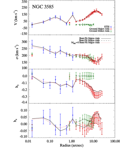
Figure 1.— Gauss–Hermite moments of LOSVDs for NGC 3585. Blue crosses are Gauss–Hermite moments of LOSVDs from HST STIS data. Also plotted are ground-based Gauss–Hermite moments of LOSVDs along the major axis (red diamonds) and minor axis (green triangles) from Fisher (1997). Fisher (1997) binned $v$ and $\sigma$ differently from the third and fourth moments. We interpolated and rebinned them consistently. Because the ground $h_{3}$ and $h_{4}$ moments have been interpolated, their error bars are larger than their scatter. Though Gauss–Hermite moments are not fitted directly in the modeling, the jagged black lines are the resulting Gauss–Hermite fit to the best-fit model’s LOSVDs from § 3 for the major axis (solid black) and minor axis (dashed black). The best-fit model has $M_{\mathrm{BH}}=3.4\times 10^{8}~{}{\mathrm{M}}_{\scriptscriptstyle\odot}$ and $\Upsilon=3.5$. The STIS spectra show a rise in velocity dispersion toward the center and require a black hole to match the increased mass-to-light ratio. The red dotted line shows the best-fit model for which $M_{\mathrm{BH}}=0$, which has $\Upsilon=4.1$.

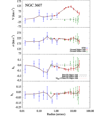
Figure 2.— Gauss–Hermite moments of LOSVDs for NGC 3607. Symbols are as in Figure 1. Ground-based data are from Bender et al. (1994). The best-fit model (black lines) has $M_{\mathrm{BH}}=1.25\times 10^{8}~{}{\mathrm{M}}_{\scriptscriptstyle\odot}$ and $\Upsilon=7.3$. The best-fit model without a black hole (red, dotted line) has $\Upsilon=7.5$.

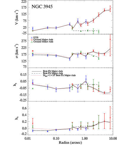
Figure 3.— Gauss–Hermite moments of LOSVDs for NGC 3945. Symbols are as in Figure 1. Ground data are from our MDM observations. Error bars for ground-based data are from variations from one side of the galaxy to the other, which dominate the total uncertainty for this galaxy. The black jagged lines are from the best-fit model, which has $M_{\mathrm{BH}}=0$ and $\Upsilon=7.2$.

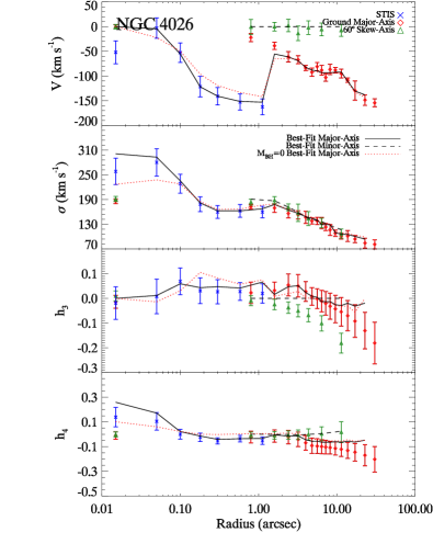
Figure 4.— Gauss–Hermite moments of LOSVDs for NGC 4026. Symbols are as in Figure 1. Ground-based data are from Fisher (1997), for which the $h_{3}$ and $h_{4}$ moments have been interpolated. Because of the interpolation, the scatter in the data is less than the error bars. The LOSVDs show a sharp increase in velocity dispersion toward the center. The jagged lines are from the best-fit model, which has $M_{\mathrm{BH}}=2.2\times 10^{8}~{}{\mathrm{M}}_{\scriptscriptstyle\odot}$ and $\Upsilon=4.6$. The best-fit model without a black hole (red dotted line) has $\Upsilon=5.6$.

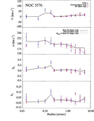
Figure 5.— Gauss–Hermite moments of LOSVDs for NGC 5576. Symbols are as in Figure 1. The ground-based data are from our Magellan observations. The jagged lines are from the best-fit model, which has $M_{\mathrm{BH}}=1.6\times 10^{8}~{}{\mathrm{M}}_{\scriptscriptstyle\odot}$ and $\Upsilon=3.6$. The best-fit model without a black hole (red dotted line) has $\Upsilon=4.0$.

3. Dynamical Models to Estimate $M_{\mathrm{BH}}$

In this section we present the results of models to test for the presence of a central black hole. We use the three-integral, axisymmetric Schwarzschild method to make dynamical models of the galaxies. The method is explained by Gebhardt et al. (2003) and in more detail by Siopis et al. (2008), but we very briefly outline it here.

First, we use the photometric data with the assumption of axisymmetry and a given inclination to find the luminosity density of the galaxy. We use the luminosity density with a given mass-to-light ratio ($\Upsilon$) and a given black hole mass to calculate the potential. We then calculate the orbits of representative stars in this potential. From this, we determine the weights for the set of orbits that best reproduces the surface-brightness profile. With the weighted orbit library, we find the LOSVD for a given inclination for comparison with the observed spectra.

The results are summarized in Table 5. For all galaxies, we modeled several inclination angles, but in all cases none was clearly preferred by the models alone, and all found the same black hole mass within the stated uncertainties. We present the values from our edge-on models below except for NGC 3607, whose image indicates that it is face-on. Measurement errors are 1$\sigma$ uncertainties. We generally report two values for black hole mass and mass-to-light ratio in the text: (1) the best-fit-model value which comes from the single model with the smallest $\chi^{2}$ and (2) the value obtained from marginalizing over the other parameter. These two values are not always exactly equal, but the best-fit model is always within 1$\sigma$ of the marginalized value. We put the marginalized values, which incorporate our uncertainty in the other parameter, in Table 5 and use those values for all subsequent calculations.

We have investigated the reliability of this orbit-superposition program in a number of ways. The results from the program have been compared to those from the Leiden program developed by McDermid et al. (in preparation), giving consistent results for NGC 0821 using the different codes on the same data and on different data of the same galaxy. Siopis et al. (2008) also tested our method by synthesizing a distribution function for a galaxy and running them through the modeling program. The models were able to recover the black hole mass as well as the orbital configuration.

Gebhardt (2004) demonstrated that a sufficiently large orbit library produces consistent results with other orbit libraries of similar or larger sizes. He showed that the black hole mass is not influenced by the choice of the weight on entropy in the solution process, provided it is sufficiently small. Gebhardt et al. (2003) also showed that a set of objects observed at HST resolution and ground-based resolution gives consistent (but with different precisions) black hole masses when only the ground-based data are used to construct models. Kormendy (2004) showed that estimates of the mass of the black hole in M32 using techniques similar to these but different in detail give results consistent with the current value (and their own error bars) over a 10-fold improvement in spatial resolution. Hence, in the context of these models we believe the program returns correct estimates of black hole mass and mass-to-light ratio, and we adopt these estimates below, even when the radius of influence of the resulting black hole, $R_{\mathrm{infl}}=GM_{\mathrm{BH}}/\sigma^{2}(R_{\mathrm{infl}})$, is less than the resolution of the observation.

There are at least three issues that might lead us to report black hole masses that are significantly wrong (i.e., outside our error bars). First, the models are axisymmetric by construction, hence significant triaxiality could lead to an error. Triaxial models, of course, can reconstruct the correct structure (e.g., van den Bosch et al., 2008). Second, the models are assumed to have constant stellar mass-to-light ratios except for the central black hole. An admixture of dark matter with a spatial distribution different from that of the luminous matter could lead us to determine an incorrect black hole mass thus requiring dark matter in the model (e.g., Thomas et al., 2007). Finally, Houghton et al. (2006) have argued for methods of determining the LOSVD that address the limitation of our method (maximum penalized likelihood)—that it produces LOSVDs with correlated errors. Gebhardt et al. (2003) did Monte Carlo simulations that give us confidence in our ability to estimate the number of independent data in our LOSVDs. Nonetheless, our method could be improved.

Table 5Mass Measurements

Galaxy	$\sigma_{e}$	$M_{\mathrm{BH}}$	$M_{\mathrm{BH,low}}$	$M_{\mathrm{BH,high}}$	$\Upsilon_{V}$	$\chi^{2}$	$\Delta\chi^{2}$
NGC 3585	213	$3.4\times 10^{8}$	$2.8\times 10^{8}$	$4.9\times 10^{8}$	3.4 $\pm$ 0.2	55.8	28.7
NGC 3607	229	$1.2\times 10^{8}$	$7.9\times 10^{7}$	$1.6\times 10^{8}$	7.5 $\pm$ 0.3	69.1	10.6
NGC 3945	192	$9\times 10^{6}$	$-1.2\times 10^{7}$	$2.6\times 10^{7}$	6.6 $\pm$ 0.8	46.2	. . . .
NGC 4026	180	$2.1\times 10^{8}$	$1.7\times 10^{8}$	$2.8\times 10^{8}$	4.5 $\pm$ 0.3	78.7	26.2
NGC 5576	183	$1.8\times 10^{8}$	$1.4\times 10^{8}$	$2.1\times 10^{8}$	3.7 $\pm$ 0.3	319.1	15.5

Note. — Results from mass modeling. Effective stellar velocity dispersions are given in units of $~{}\mathrm{km~{}s^{-1}}$, masses are in units of ${\mathrm{M}}_{\scriptscriptstyle\odot}$, and $\Upsilon_{V}$ is units of ${\mathrm{M}}_{\scriptscriptstyle\odot}~{}{\mathrm{L}}^{-1}_{\scriptscriptstyle\odot,V}$. The black hole masses and mass-to-light ratios are the result of marginalizing over the other parameter. $M_{\mathrm{BH,low}}$ and $M_{\mathrm{BH,high}}$ are the 1$\sigma$ confidence limits on the detected black hole mass. The final two columns list $\chi^{2}$ of the best-fit model, and the difference between the minimum in the marginalized $\chi^{2}$ and at $M_{\mathrm{BH}}=0$.

3.1. NGC 3585

NGC 3585 (catalog NGC 3585) is an edge-on S0 galaxy at a distance of $21.2~{}\mathrm{Mpc}$ (de Vaucouleurs et al., 1991; Tonry et al., 2001). Images of the galaxy show that it is flattened with a nearly edge-on dust ring at its center. The LOSVD profile shows a roughly constant velocity dispersion from about $1\arcsec$ to $\sim 6\arcsec$ of $\sigma\approx 200~{}\mathrm{km~{}s^{-1}}$. Inside $\sim 0\farcs 1$ the dispersion rises to $\sim 280~{}\mathrm{km~{}s^{-1}}$, indicating a likely increase of mass-to-light ratio toward the center. For use in analysis of the $M$–$\sigma$ relation, we compute an effective stellar velocity dispersion,

$$\sigma^{2}_{e}\equiv\frac{\int_{0}^{R_{e}}\left({\sigma^{2}+V^{2}}\right)I\left(r\right)dr}{{\int_{0}^{R_{e}}I\left(r\right)dr}},$$ (3)

where $R_{e}$ is the effective radius, $I(r)$ is the surface-brightness profile, and $V$ and $\sigma$ are the first and second Gauss–Hermite moments of the LOSVD from a slit of width 1″. From the ground-based velocity profile, we find an effective stellar velocity dispersion of $\sigma_{e}=213~{}\mathrm{km~{}s^{-1}}$.

The $\chi^{2}$ contours in the $M_{\mathrm{BH}}$–$\Upsilon$ plane are plotted in Figure 6. The best-fitting model is able to reproduce all of the major features in the velocity profile, and in order to produce the increase in velocity dispersion seen toward the center, a black hole is required. The velocity profiles for the best-fit models are shown in Figure 1. We marginalize over mass-to-light ratio and take $\Delta\chi^{2}=1$ as our $1\sigma$ uncertainty to find a black hole mass of $M_{\mathrm{BH}}=3.4{}_{-0.6}^{+1.5}\times 10^{8}~{}{\mathrm{M}}_{\scriptscriptstyle\odot}$. For $M_{\mathrm{BH}}=0$, the marginalized $\chi^{2}$ increases from the minimum by 28.7, which rules out the absence of a black hole at very high significance (better than $99.99\%$ confidence). Marginalizing over black hole mass, we find a $V$-band mass-to-light ratio $\Upsilon_{V}=3.4\pm 0.2$. The best-fit model with $M_{\mathrm{BH}}=3.4\times 10^{8}~{}{\mathrm{M}}_{\scriptscriptstyle\odot}$ and $\Upsilon=3.5$ has $\chi^{2}=55.8$. The difference between the best-fit model and the best-fit model with $M_{\mathrm{BH}}=0$ is not obvious in Figure 1, which shows the Gauss–Hermite moments of the LOSVDs. For this reason, we present a plot of the cumulative difference in $\chi^{2}$ between the two models in Figure 7. The value for $\Delta\chi^{2}$ is different from the value shown in Table 5, which reports the difference in marginalized $\chi^{2}$ whereas Figure 7 is the difference between two individual models. The best-fit model generally differs from the best-fit model without a black hole by a larger amount. The cumulative $\chi^{2}$ plot shows that most of the difference comes from the central $\sim 1\arcsec$.

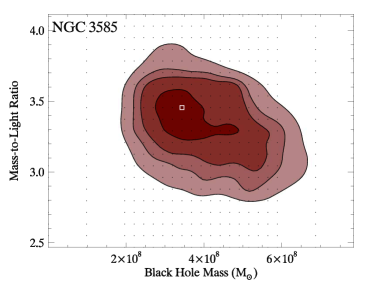
Figure 6.— Mass modeling $\chi^{2}$ contours for NGC 3585, assuming edge-on inclination. Contours are for $\Delta\chi^{2}=$ 1.00, 2.71, 4.00, and 6.63, which bracket individual parameter confidence levels of 68.3, 90.0, 95.4, and 99.0%, respectively. Contours have been smoothed for plotting. The square shows the best-fit model. Dots indicate parameters modeled. The contours were smoothed for plotting. The best-fit model has $M_{\mathrm{BH}}=3.4\times 10^{8}~{}{\mathrm{M}}_{\scriptscriptstyle\odot}$ and $\Upsilon=3.5$. Marginalizing over the other parameter we find $M_{\mathrm{BH}}=3.4^{+2.5}_{-0.6}\times 10^{8}~{}{\mathrm{M}}_{\scriptscriptstyle\odot}$ and $\Upsilon=3.4\pm 0.2$.

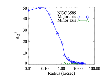
Figure 7.— Cumulative $\chi^{2}$ difference between the best-fit model ($M_{\mathrm{BH}}=3.4\times 10^{8}~{}{\mathrm{M}}_{\scriptscriptstyle\odot}$ and $\Upsilon=3.5$) and the best-fit model without a black hole in NGC 3585. The difference in $\chi^{2}$ is summed from the outermost region to the innermost for each axis. Positive $\Delta\chi^{2}$ indicates that the model with a black hole is preferred. The total difference in $\chi^{2}$ is different from the value listed in Table 5 because this difference is between the two individual models rather than the marginalized results. Most of the difference comes from the inner 1″.

3.2. NGC 3607

NGC 3607 (catalog NGC 3607) is an elliptical galaxy at a distance of $19.9~{}\mathrm{Mpc}$ (de Vaucouleurs et al., 1991; Tonry et al., 2001). The galaxy has a nearly opaque dust disk toward the center (Lauer et al., 2005), and the image indicates a nearly face-on profile. For this galaxy we assumed an inclination angle of $51^{\circ}$, corresponding to a true axis ratio of 0.4. The dust obscures a large part of the bulge, but the nucleus is still visible and is thus suitable for modeling. The velocity dispersion is roughly flat with radius, but there is an increased rotation in the inner 0$\farcs$1, indicating a dark mass. The effective stellar velocity dispersion $\sigma_{e}=229~{}\mathrm{km~{}s^{-1}}$. The $\chi^{2}$ contours in the $M_{\mathrm{BH}}$-$\Upsilon$ plane are plotted in Figure 8. The velocity profiles for the best-fit models are shown in Figure 2. Marginalizing over $\Upsilon$, we find a black hole mass of $M_{\mathrm{BH}}=1.2{}_{-0.4}^{+0.4}\times 10^{8}~{}{\mathrm{M}}_{\scriptscriptstyle\odot}$. For $M_{\mathrm{BH}}=0$, the marginalized $\chi^{2}$ increases from the minimum by 10.6, which rules out the absence of a black hole at the $99.9\%$ confidence level. Marginalizing over black hole mass, we find a $V$-band mass-to-light ratio $\Upsilon_{V}=7.5\pm 0.3$. The best-fit model with $M_{\mathrm{BH}}=1.25\times 10^{8}~{}{\mathrm{M}}_{\scriptscriptstyle\odot}$ and $\Upsilon=7.3$ has $\chi^{2}=69.12$. Figure 9 shows the cumulative $\chi^{2}$ as a function of radius, which indicates that most of the difference comes from the central $\sim 1\arcsec$.

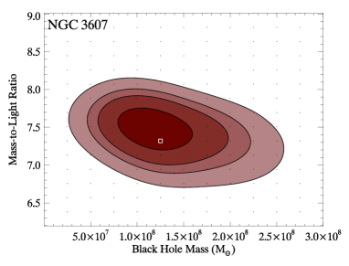
Figure 8.— Mass modeling $\chi^{2}$ contours for NGC 3607, assuming an inclination of $51^{\circ}$. Contours are the same as in Figure 6. Contours have been smoothed for plotting. The best-fit model has $M_{\mathrm{BH}}=1.25\times 10^{8}~{}{\mathrm{M}}_{\scriptscriptstyle\odot}$ and $\Upsilon=7.3$. Marginalizing over the other parameter, we find $M_{\mathrm{BH}}=1.2^{+0.4}_{-0.4}\times 10^{8}~{}{\mathrm{M}}_{\scriptscriptstyle\odot}$ and $\Upsilon=7.5\pm 0.3$.

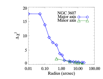
Figure 9.— Same as Figure 7 but for NGC 3607. Positive values of $\Delta\chi^{2}$ indicate preference for the best-fit model ($M_{\mathrm{BH}}=1.25\times 10^{8}~{}{\mathrm{M}}_{\scriptscriptstyle\odot}$ and $\Upsilon=7.3$). Most of the difference comes from the central 1″.

3.3. NGC 3945

At a distance of $19.9~{}\mathrm{Mpc}$, NGC 3945 (catalog NGC 3945) is an SB0 galaxy with a pseudobulge (de Vaucouleurs et al., 1991; Tonry et al., 2001; Lauer et al., 2007b; Kormendy & Kennicutt, 2004). This galaxy also contains both an inner bar system and an inner disk (e.g., Erwin, 2004; Erwin & Sparke, 1999). The bars may present problems four our axisymmetric code, which we discuss in § 4. The velocity profile shows a rise in velocity dispersion toward the center from $r=0\farcs 2$, but this may also be interpreted as a slight dip in velocity dispersion at $r\approx 0\farcs 2$–$0\farcs 3$. It has an effective stellar velocity dispersion $\sigma_{e}=192~{}\mathrm{km~{}s^{-1}}$. The velocity profiles for the best-fit models are shown in Figure 3.

The $\chi^{2}$ contours in the $M_{\mathrm{BH}}$-$\Upsilon$ plane are plotted in Figure 10. The results of the kinematic modeling show that this galaxy is consistent with no black hole at its center. Marginalizing over $\Upsilon$, our estimates of the black hole mass for any inclination do not exclude a black hole mass of zero at the 1$\sigma$ level: $M_{\mathrm{BH}}=9{}_{-21}^{+17}\times 10^{6}~{}{\mathrm{M}}_{\scriptscriptstyle\odot}$. The 2$\sigma$ upper limit is $M_{\mathrm{BH}}<3.8\times 10^{7}~{}{\mathrm{M}}_{\scriptscriptstyle\odot}$, and the 3$\sigma$ upper limit is $M_{\mathrm{BH}}<5.1\times 10^{7}~{}{\mathrm{M}}_{\scriptscriptstyle\odot}$.

Because $M_{\mathrm{BH}}=0$ was allowed for this galaxy, we included negative black hole masses in our parameter space coverage. This let us consider the full extent of the 1$\sigma$ error distribution on the low-mass side. Our model allows a negative black hole mass as long as the total mass inside the smallest pericenter of the orbit library is positive. In essence, this produces a delta function decrement to the mass density.

The sphere of influence of the black holes of the mass we find is below the resolution limit of our data. The black hole mass for $R_{\mathrm{infl}}/r_{\mathrm{res}}=0.5$ is $M_{\mathrm{BH}}=D\;\theta_{\mathrm{res}}{\sigma}^{2}/G=9.7\times 10^{7}~{}{\mathrm{M}}_{\scriptscriptstyle\odot}$, where $D$ is the distance to the galaxy and $\theta_{\mathrm{res}}=0\farcs 05$ is the spatial resolution limit of the spectra. Such a black hole mass, however, is ruled out by our modeling under our assumptions of constant mass-to-light ratio and axisymmetry, as inside $0\farcs 1$ it would produce an excess velocity dispersion above that observed, especially in the central STIS pixel. Marginalizing over black hole mass, we find $\Upsilon_{V}=6.6\pm 0.8$. The model with $M_{\mathrm{BH}}=-2.5\times 10^{6}~{}{\mathrm{M}}_{\scriptscriptstyle\odot}$ and $\Upsilon=6.8$ has $\chi^{2}=45.4$. Figure 11 shows the cumulative $\chi^{2}$ as a function of radius, which indicates that most of the difference comes from the central $\sim 0\farcs 1$.

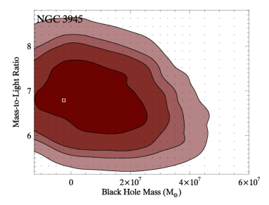
Figure 10.— Mass modeling $\chi^{2}$ contours for NGC 3945, assuming edge-on inclination. Contours are as in Figure 6. Contours have been smoothed for plotting. The best-fit model has $M_{\mathrm{BH}}=-2.5\times 10^{6}~{}{\mathrm{M}}_{\scriptscriptstyle\odot}$ and $\Upsilon=6.8$. Marginalizing over the other parameter we find $M_{\mathrm{BH}}=9^{+17}_{-21}\times 10^{6}~{}{\mathrm{M}}_{\scriptscriptstyle\odot}$ and $\Upsilon=6.6\pm 0.8$.

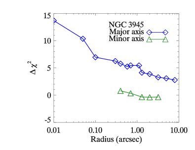
Figure 11.— Same as Figure 7 but for NGC 3945. Positive values of $\Delta\chi^{2}$ indicate preference for the best-fit model ($M_{\mathrm{BH}}=0$ and $\Upsilon=8.4$) compared to the best-fit model with $M_{\mathrm{BH}}=1.0\times 10^{8}~{}{\mathrm{M}}_{\scriptscriptstyle\odot}$, the mass for a marginally resolved sphere of influence. Most of the difference comes from the central 0$\farcs$1.

3.4. NGC 4026

NGC 4026 (catalog NGC 4026) is an S0 galaxy at a distance of $15.6~{}\mathrm{Mpc}$ (de Vaucouleurs et al., 1991; Tonry et al., 2001). Images show a very flattened profile, indicating that edge-on models are appropriate for this galaxy. There is also a weak, cold stellar disk in the center. The spectra show a flat velocity dispersion from $r\approx 3$″to $r\approx 0\farcs 3$ of $\sigma\approx 160~{}\mathrm{km~{}s^{-1}}$ Inside 0$\farcs$3, the velocity dispersion increases quickly to $\sigma=258~{}\mathrm{km~{}s^{-1}}$ at the center, a strong indication of increased mass-to-light ratio. The effective stellar velocity dispersion $\sigma_{e}=180~{}\mathrm{km~{}s^{-1}}$.

The $\chi^{2}$ contours in the $M_{\mathrm{BH}}$-$\Upsilon$ plane are plotted in Figure 12. The velocity profiles for the best-fit models are shown in Figure 4. Marginalizing over $\Upsilon$, we find a black hole mass of $M_{\mathrm{BH}}=2.1{}_{-0.4}^{+0.7}\times 10^{8}~{}{\mathrm{M}}_{\scriptscriptstyle\odot}$. For $M_{\mathrm{BH}}=0$, the marginalized $\chi^{2}$ increases from the minimum by 26.2. Such an increase in $\Delta\chi^{2}$ rules out the absence of a black hole at a confidence level greater than $99.99\%$. Marginalizing over black hole mass, we find $\Upsilon_{V}=4.5\pm 0.3$. The best-fit model with $M_{\mathrm{BH}}=2.2\times 10^{8}~{}{\mathrm{M}}_{\scriptscriptstyle\odot}$ and $\Upsilon=4.6$ has $\chi^{2}=78.7$. Figure 13 shows the cumulative $\chi^{2}$ as a function of radius, which indicates that most of the difference comes from the central $\sim 1\arcsec$.

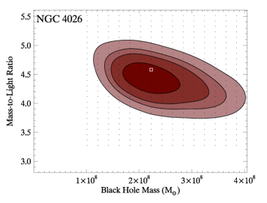
Figure 12.— Mass modeling $\chi^{2}$ contours for NGC 4026, assuming edge-on inclination. Contours are as in Figure 6. Contours have been smoothed for plotting. The best-fit model has $M_{\mathrm{BH}}=2.2\times 10^{8}~{}{\mathrm{M}}_{\scriptscriptstyle\odot}$ and $\Upsilon=4.6$. Marginalizing over the other parameter we find $M_{\mathrm{BH}}=2.1^{+0.7}_{-0.4}\times 10^{8}~{}{\mathrm{M}}_{\scriptscriptstyle\odot}$ and $\Upsilon=4.5\pm 0.3$.

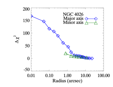
Figure 13.— Same as Figure 7 but for NGC 4026. Positive values of $\Delta\chi^{2}$ indicate preference for the best-fit model ($M_{\mathrm{BH}}=2.2\times 10^{8}~{}{\mathrm{M}}_{\scriptscriptstyle\odot}$ and $\Upsilon=4.6$). Most of the difference comes from the central 1″.

3.5. NGC 5576

NGC 5576 (catalog NGC 5576) is an E3 radio galaxy at a distance of $27.1~{}\mathrm{Mpc}$ (de Vaucouleurs et al., 1991; Tonry et al., 2001). The nucleus is offset by $\sim 0\farcs 04$ from the center of the outer isophotes (Lauer et al., 2005). Our ground-based spectroscopy qualitatively confirms this, showing that the central region is kinematically separate from the outer regions. The ground-based spectroscopy reveals an effective stellar velocity dispersion of $\sigma_{e}=183~{}~{}\mathrm{km~{}s^{-1}}$. Unlike the other modeling, for this galaxy we did not average both sides of galaxy for the ground-based data. Instead, we included data from both sides of the galaxy with the sign of the velocity appropriately changed on one side. Figure 14 shows the $\chi^{2}$ contours from dynamical models. The velocity profiles for the best-fit models are shown in Figure 5. Marginalizing over $\Upsilon$, we find a black hole mass of $M_{\mathrm{BH}}=1.8{}_{-0.4}^{+0.3}\times 10^{8}~{}{\mathrm{M}}_{\scriptscriptstyle\odot}$. At $M_{\mathrm{BH}}=0$, the marginalized $\chi^{2}$ increases 15.5 above the minimum, indicating that $M_{\mathrm{BH}}=0$ is ruled out at the $99.99\%$ confidence level. Marginalizing over black hole mass, we nominally find $\Upsilon_{V}=3.7\pm 0.3$. The best-fit model with $M_{\mathrm{BH}}=1.6\times 10^{8}{\mathrm{M}}_{\scriptscriptstyle\odot}$ and $\Upsilon=3.6$ has $\chi^{2}=319.3$. The value for $\chi^{2}$ is much larger than it is for the other galaxies because (1) the ground-based data come from 13 velocity bins instead of four Gauss–Hermite moments, resulting in more constraints, and (2) there are two sets of LOSVDs for each ground-based axis measurement: one from each side of the galaxy. Figure 15 shows the cumulative $\chi^{2}$ as a function of radius, which indicates that most of the difference comes from the central $\sim 0\farcs 2$.

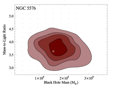
Figure 14.— Mass modeling $\chi^{2}$ contours for NGC 5576, assuming edge-on inclination. Contours are as in Figure 6. Contours have been smoothed for plotting. The best-fit model has $M_{\mathrm{BH}}=1.6\times 10^{8}~{}{\mathrm{M}}_{\scriptscriptstyle\odot}$ and $\Upsilon=3.6$. Marginalizing over the other parameter, we find $M_{\mathrm{BH}}=1.8^{+0.3}_{-0.4}\times 10^{8}~{}{\mathrm{M}}_{\scriptscriptstyle\odot}$ and $\Upsilon=3.7\pm 0.3$.

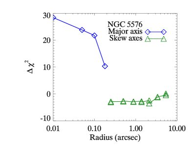
Figure 15.— Same as Figure 7 but for NGC 5576. Positive values of $\Delta\chi^{2}$ indicate preference for the best-fit model ($M_{\mathrm{BH}}=1.6\times 10^{8}~{}{\mathrm{M}}_{\scriptscriptstyle\odot}$ and $\Upsilon=3.6$). Most of the difference comes from the central 0$\farcs$2.

4. Discussion and Summary

It is worth emphasizing that our modeling gives results for massive dark objects at the centers of galaxies, which we call “black holes.” Though the cumulative evidence in favor of these central dark masses as black holes is strong, alternatives can only be ruled out for the most highly resolved sources: the Galaxy, M31, and NGC 4258 (e.g., Miller, 2006). Thus, while a large black hole is the most astrophysically likely explanation of these central dark objects, they do not strictly have to be black holes.

Our models assume a constant mass-to-light ratio for the stellar component of the galaxy. One possible source of systematic error may come from the role that dark matter halos play. Dark matter halos likely increase the total mass-to-light ratio in the outer parts of the galaxy but have less of an impact toward the center. Thus, by neglecting the dark matter halo, we may be overestimating the stellar mass-to-light ratio at the center of the galaxy and, consequently, underestimating the black hole mass. Future models will incorporate dark matter halos.

Another assumption of ours that may be violated is that of axisymmetry. Triaxiality has been addressed in other models (van den Bosch et al., 2008). In addition to triaxiality are bars, which affect NGC 3945, a double-barred system. While the primary bar is not prominent inside of $15\arcsec$, where all of our kinematic data come from, box orbits from bars can travel to the center. Our modeling code is axisymmetric and simply cannot model bars. It is possible that our modeling results, including the mass of the black hole, are skewed by the bars. If the bar is aligned mostly along the line of sight, then the line-of-sight velocity would be higher than without the bar. The higher velocities, which would be observed, could be misinterpreted as extra dark mass since the bar orbits would not be accounted for in the model. On the other hand, if the bar is aligned mostly perpendicularly to the line of sight, the bar orbits would contribute little to the line-of-sight velocity at the center, leading to an underestimate in central dark mass. One of the bars in NGC 3945 appears to lie in the plane of the sky, and one of the bars is at least partially along the line of sight, assuming that they are coplanar with the outer disk. Thus it is entirely possible that the bars are leading to an incorrect inference of the black hole mass, but it is not obvious whether it is skewed to a high or low value.

4.1. Anisotropy

In Figures 16–20, we show the velocity dispersion tensor for the best-fit model for each galaxy by plotting the ratio of the radial velocity dispersion ($\sigma_{r}$) to the tangential velocity dispersion, defined as $\sigma_{t}^{2}\equiv 0.5(\sigma_{\theta}^{2}+\sigma_{\phi}^{2})$ so that $\sigma_{r}/\sigma_{t}=1$ for an isotropic distribution. Here, $\sigma_{\phi}$ is the second moment of the azimuthal velocity relative to the systemic velocity rather than relative to the mean rotational speed. Uncertainties may be estimated from the smoothness of the profiles (Gebhardt et al., 2003) to be $0.1$ to $0.3$. All galaxies are dominated by tangential motion at the center.

NGC 3585 (Figure 16) has an intermediate surface-brightness profile and actually shows $\sigma_{r}/\sigma_{t}$ mildly increasing toward the center along the major axis, but with a steep decrease inside of 0$\farcs$1 along the minor axis. For almost the entire range out to 23″, $\sigma_{r}/\sigma_{t}<1$.

The two core-profile galaxies, NGC 3607 (Figure 17) and NGC 5576 (Figure 20), are both ellipticals and show near-isotropic distributions in the outer regions, but both galaxies are dominated by tangential motion at the center. For NGC 3607, the radial motion drops to almost zero. NGC 3607 has a relatively strong velocity gradient across the central 0$\farcs$3, and it has a strong drop in the velocity dispersion in the center. The only way to reproduce these observables is to have complete tangential anisotropy, i.e., no radial orbits.

The other two galaxies, NGC 3945 (Figure 18) and NGC 4026 (Figure 19) are S0 galaxies with power-law profiles. For NGC 3945, outside of 10″, where the kinematic data end, radial anisotropy dominates, but the uncertainties are large here (Gebhardt et al., 2003). Inside of 10″, the dispersion along the major axis steadily decreases from a roughly isotropic value to $\sigma_{r}/\sigma_{t}\approx 0.5$. The dispersion along the minor axis jumps from tangential to radial at $r\approx 3\arcsec$ and then steadily decreases to $\sigma_{r}/\sigma_{t}\approx 0.7$. NGC 4026 shows $\sigma_{r}/\sigma_{t}<1$ almost everywhere.

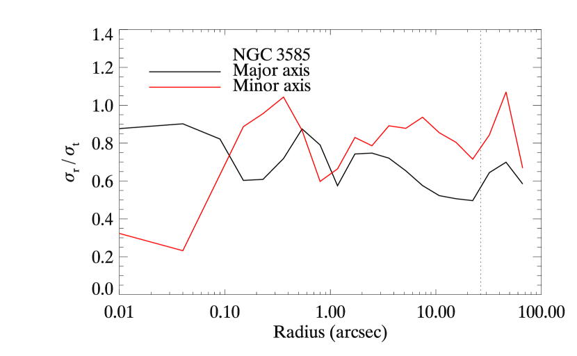
Figure 16.— Shape of the velocity dispersion tensor for NGC 3585 from the best-fit model orbit solution. The black line is along the major axis, and the red line is along the minor axis. The values for the central part of the galaxy are plotted at a radius of 0$\farcs$01. The dotted line shows the radial extent of the ground-based spectroscopic data.

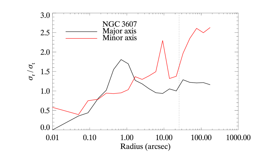
Figure 17.— Same as Figure 16 but for NGC 3607.

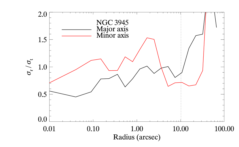
Figure 18.— Same as Figure 16 but for NGC 3945.

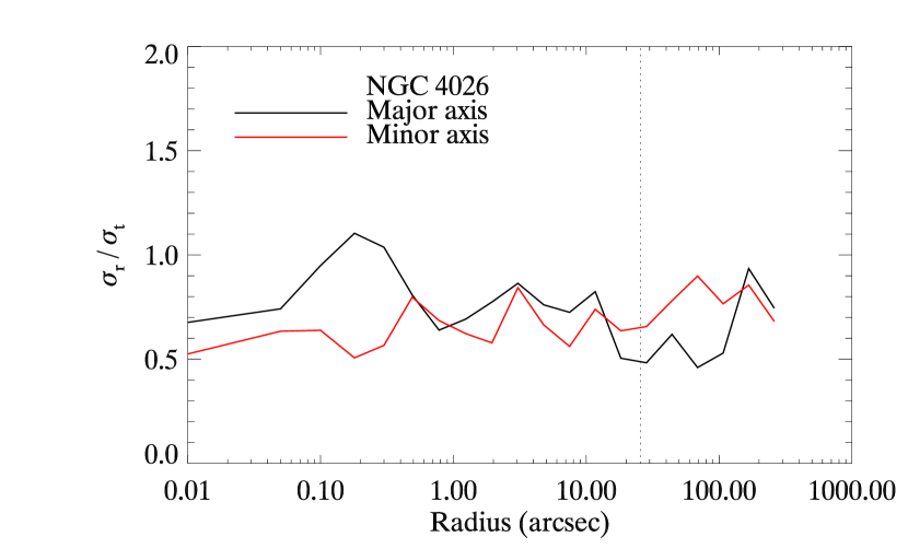
Figure 19.— Same as Figure 16 but for NGC 4026.

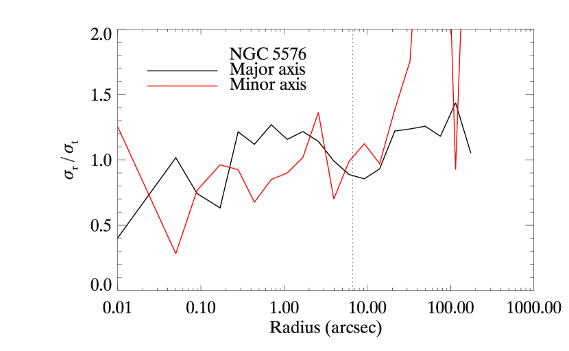
Figure 20.— Same as Figure 16 but for NGC 5576.

4.2. Demographics

We plot the masses found in § 3 against $\sigma_{e}$ and $L_{V}$ in Figure 21, along with the $M$–$\sigma$ and $M$–$L$ relations from Tremaine et al. (2002) and Lauer et al. (2007b), respectively. With the exception of NGC 3585 in Figure 21(b), all of the black hole masses differ from the values predicted by the scaling relations by at least 1$\sigma$. This shows that our black hole mass measurements are precise enough to probe the intrinsic scatter in these relations. The measurement of the intrinsic scatter in these relations is addressed by Gültekin et al. (2009). If unaccounted systematic errors are large, however, the residual scatter could be due to these. Random errors in distance are unlikely to be a large part of this as they are typically 10%, which is substantially smaller than the $\sim 2$ deviation from the $M$–$\sigma$ ridgeline. For these particular galaxies, inclination does not appear to make a significant difference in black hole mass. Systematic errors from triaxiality or bars, however, are difficult to estimate and may contribute.

If one assumes an intrinsic scatter of 0.3 dex in the $M$–$\sigma$ relation (the maximum intrinsic scatter found by Tremaine et al., 2002) and 0.5 dex in the $M$–$L$ relation (Lauer et al., 2007a), all black hole masses are consistent with the scaling relations except for NGC 3945, which is significantly below both relations. The black hole masses expected for NGC 3945 from the $M$–$\sigma$ and $M$–$L$ relations are $1.1\times 10^{8}~{}{\mathrm{M}}_{\scriptscriptstyle\odot}$ and $1.6\times 10^{8}~{}{\mathrm{M}}_{\scriptscriptstyle\odot}$, respectively. The 3$\sigma$ upper limit for NGC 3945 is $M_{\mathrm{BH}}<5.1\times 10^{7}~{}{\mathrm{M}}_{\scriptscriptstyle\odot}$. Hence, while it not possible to rule out the existence of a small black hole in NGC 3945, it does not fall on the $M$–$\sigma$ or $M$–$L$ relations.

Figure 21.— Plots of black hole masses as functions of the host galaxies’ effective stellar velocity dispersion (left) and luminosity (right). The lines are the $M$–$\sigma$ relation from Tremaine et al. (2002) (left) and the $M$–$L$ relation from Lauer et al. (2007b) (right). With the exception of NGC 3945, all masses are found near the lines, but they are all inconsistent with the best-fit $M$–$\sigma$ relation at the 1$\sigma$ level, and all but NGC 3585 are inconsistent with the $M$–$L$ line. Given the estimated scatter in the relations, most of the black hole masses follow the relation. NGC 3945, however, is significantly below the relations. Even the 3$\sigma$ upper limit to its mass ($M_{\mathrm{BH}}<5.1\times 10^{7}~{}{\mathrm{M}}_{\scriptscriptstyle\odot}$) is more than a factor of 2 below the expected $1.1\times 10^{8}~{}{\mathrm{M}}_{\scriptscriptstyle\odot}$ from $M$–$\sigma$ and $1.6\times 10^{8}~{}{\mathrm{M}}_{\scriptscriptstyle\odot}$ from $M$–$L$.

It is interesting to note that the single galaxy in our sample that is consistent with having no black hole, NGC 3945, is a pseudobulge. Comparing fits to the $M$–$\sigma$ relation of pseudobulges with normal bulges and ellipticals, Hu (2008) concluded that pseudobulges have systematically smaller black holes. The small or absent black hole in NGC 3945 is consistent with those findings.

4.3. Summary

We conclude by summarizing the main results of this paper. We observed five early-type galaxies with high spatial resolution kinematics from STIS, which we combined with WFPC2 photometry and ground-based observations of photometry and kinematics. We modeled these data with three-integral, axisymmetric orbit models and found a black hole mass consistent with zero and significantly below the $M$–$\sigma$ and $M$–$L$ relations in one,

$$\mathrm{NGC~{}3945} : ~{}M_{\mathrm{BH}}=9^{+17}_{-21}\times 10^{6}~{}{\mathrm{M}}_{\scriptscriptstyle\odot},$$

though the presence of a double bar in this galaxy may present problems for our axisymmetric code. We find evidence for central black holes in the remaining four:

$$\mathrm{NGC~{}3585} : ~{}M_{\mathrm{BH}}=3.4^{+1.5}_{-0.6}\times 10^{8}~{}{\mathrm{M}}_{\scriptscriptstyle\odot},$$

$$\mathrm{NGC~{}3607} : ~{}M_{\mathrm{BH}}=1.2^{+0.4}_{-0.4}\times 10^{8}~{}{\mathrm{M}}_{\scriptscriptstyle\odot},$$

$$\mathrm{NGC~{}4026} : ~{}M_{\mathrm{BH}}=2.1^{+0.7}_{-0.4}\times 10^{8}~{}{\mathrm{M}}_{\scriptscriptstyle\odot},$$

and

$$\mathrm{NGC~{}5576} : ~{}M_{\mathrm{BH}}=1.8^{+0.3}_{-0.4}\times 10^{8}~{}{\mathrm{M}}_{\scriptscriptstyle\odot}.$$

In all of these last four galaxies, the absence of a central dark object is ruled out to very high significance.

This Appendix gives tables of the original data used in this paper. Details are available in § 2.

Table 6Velocity Profile for NGC 3585

Radius	$V$		$\sigma$		$h_{3}$		$h_{4}$
0.00	$-$8.1$\pm$	31.7	281.2$\pm$	29.6	0.030$\pm$	0.069	$-$0.034$\pm$	0.061
0.05	14.3$\pm$	35.1	271.0$\pm$	36.6	$-$0.125$\pm$	0.072	$-$0.008$\pm$	0.066
0.10	73.2$\pm$	29.2	260.9$\pm$	33.5	$-$0.156$\pm$	0.067	0.044$\pm$	0.080
0.18	132.6$\pm$	29.7	193.5$\pm$	30.6	$-$0.057$\pm$	0.047	$-$0.058$\pm$	0.049
0.30	147.7$\pm$	29.5	211.2$\pm$	24.6	$-$0.181$\pm$	0.066	$-$0.010$\pm$	0.054
0.58	35.0$\pm$	25.6	213.3$\pm$	15.8	$-$0.025$\pm$	0.039	$-$0.096$\pm$	0.021
1.12	150.7$\pm$	25.7	185.8$\pm$	22.5	$-$0.109$\pm$	0.060	$-$0.015$\pm$	0.064
$-$0.05	$-$42.1$\pm$	26.9	244.4$\pm$	35.2	0.106$\pm$	0.077	0.094$\pm$	0.070
$-$0.10	$-$112.4$\pm$	29.6	185.2$\pm$	71.8	0.016$\pm$	0.115	$-$0.020$\pm$	0.151
$-$0.18	$-$88.8$\pm$	28.9	197.2$\pm$	21.1	0.024$\pm$	0.035	$-$0.060$\pm$	0.036
$-$0.30	$-$13.3$\pm$	46.5	248.6$\pm$	34.4	0.185$\pm$	0.071	$-$0.045$\pm$	0.063
$-$0.58	12.3$\pm$	37.9	198.9$\pm$	22.2	0.147$\pm$	0.054	$-$0.038$\pm$	0.037
$-$1.12	$-$104.4$\pm$	32.0	239.6$\pm$	27.5	0.320$\pm$	0.091	0.218$\pm$	0.107

Note. — Gauss–Hermite moments for velocity profiles derived from STIS data. Radii are given in arcsec, first and second moments are given in units of $\mathrm{km\;s^{-1}}$.

Table 7Velocity Profile for NGC 3607

Radius	$V$		$\sigma$		$h_{3}$		$h_{4}$
0.00	13.2$\pm$	22.8	180.5$\pm$	22.1	0.077$\pm$	0.068	$-$0.007$\pm$	0.063
$-$0.05	$-$36.1$\pm$	29.0	227.3$\pm$	35.1	0.119$\pm$	0.086	0.069$\pm$	0.111
$-$0.10	8.9$\pm$	26.3	151.4$\pm$	27.0	0.000$\pm$	0.034	$-$0.065$\pm$	0.066
$-$0.18	$-$59.9$\pm$	49.4	216.9$\pm$	39.8	$-$0.167$\pm$	0.096	$-$0.021$\pm$	0.102
$-$0.30	39.1$\pm$	33.9	206.9$\pm$	29.5	$-$0.071$\pm$	0.091	$-$0.040$\pm$	0.098
$-$0.58	22.8$\pm$	31.4	197.2$\pm$	32.3	$-$0.003$\pm$	0.079	$-$0.050$\pm$	0.072
$-$1.12	49.2$\pm$	27.5	160.2$\pm$	25.7	$-$0.011$\pm$	0.076	$-$0.031$\pm$	0.084
0.05	$-$23.3$\pm$	29.8	175.1$\pm$	28.9	0.074$\pm$	0.071	$-$0.032$\pm$	0.055
0.10	$-$67.4$\pm$	34.2	197.6$\pm$	44.4	0.117$\pm$	0.105	0.031$\pm$	0.120
0.18	$-$71.4$\pm$	28.1	169.9$\pm$	26.0	0.031$\pm$	0.050	$-$0.073$\pm$	0.036
0.30	$-$21.7$\pm$	87.7	251.7$\pm$	41.6	0.222$\pm$	0.178	$-$0.002$\pm$	0.397
0.58	$-$41.8$\pm$	44.4	261.8$\pm$	38.5	$-$0.119$\pm$	0.121	$-$0.097$\pm$	0.121
1.12	$-$27.7$\pm$	38.5	197.3$\pm$	36.3	$-$0.005$\pm$	0.083	$-$0.073$\pm$	0.073

Note. — Gauss–Hermite moments for velocity profiles derived from STIS data. Radii are given in arcsec, first and second moments are given in units of $\mathrm{km\;s^{-1}}$.

Table 8Velocity Profile for NGC 3945

Radius	$V$		$\sigma$		$h_{3}$		$h_{4}$
0.00	16.9$\pm$	10.1	170.7$\pm$	8.1	0.032$\pm$	0.036	$-$0.073$\pm$	0.030
$-$0.05	$-$14.0$\pm$	11.4	173.3$\pm$	9.8	0.058$\pm$	0.035	$-$0.100$\pm$	0.029
$-$0.10	$-$36.0$\pm$	16.9	164.4$\pm$	16.5	0.146$\pm$	0.044	$-$0.002$\pm$	0.045
$-$0.18	$-$46.6$\pm$	16.2	148.0$\pm$	18.9	0.111$\pm$	0.059	$-$0.015$\pm$	0.057
$-$0.30	$-$24.0$\pm$	18.5	125.4$\pm$	22.5	0.093$\pm$	0.058	$-$0.036$\pm$	0.062
$-$0.58	$-$100.1$\pm$	19.0	138.9$\pm$	24.2	$-$0.038$\pm$	0.073	$-$0.037$\pm$	0.079
$-$1.12	$-$29.4$\pm$	20.5	138.5$\pm$	20.5	$-$0.035$\pm$	0.057	$-$0.063$\pm$	0.075
0.05	39.5$\pm$	10.4	171.1$\pm$	9.3	0.000$\pm$	0.034	$-$0.074$\pm$	0.024
0.10	12.8$\pm$	11.8	158.6$\pm$	9.9	$-$0.021$\pm$	0.039	$-$0.075$\pm$	0.036
0.18	49.0$\pm$	13.1	121.3$\pm$	10.9	$-$0.011$\pm$	0.043	$-$0.077$\pm$	0.033
0.30	61.3$\pm$	18.0	140.5$\pm$	18.0	$-$0.053$\pm$	0.069	$-$0.025$\pm$	0.048
0.58	67.1$\pm$	19.7	167.0$\pm$	17.7	$-$0.052$\pm$	0.059	$-$0.077$\pm$	0.064
1.12	101.0$\pm$	16.1	153.6$\pm$	16.1	0.062$\pm$	0.064	$-$0.009$\pm$	0.055

Note. — Gauss–Hermite moments for velocity profiles derived from STIS data. Radii are given in arcsec, first and second moments are given in units of $\mathrm{km\;s^{-1}}$.

Table 9Velocity Profile for NGC 4026

Radius	$V$		$\sigma$		$h_{3}$		$h_{4}$
0.00	$-$52.0$\pm$	23.1	258.3$\pm$	32.0	$-$0.019$\pm$	0.066	0.139$\pm$	0.078
0.05	$-$60.0$\pm$	26.7	197.9$\pm$	27.0	$-$0.033$\pm$	0.059	$-$0.001$\pm$	0.050
0.10	$-$75.6$\pm$	27.3	197.1$\pm$	24.2	0.098$\pm$	0.050	$-$0.004$\pm$	0.050
0.18	$-$100.6$\pm$	27.0	178.8$\pm$	30.6	0.069$\pm$	0.059	0.010$\pm$	0.060
0.30	$-$79.7$\pm$	27.5	163.3$\pm$	22.0	0.048$\pm$	0.049	$-$0.057$\pm$	0.053
0.58	$-$123.2$\pm$	23.2	176.8$\pm$	21.6	0.018$\pm$	0.056	$-$0.066$\pm$	0.029
1.12	$-$105.5$\pm$	29.8	187.5$\pm$	31.6	0.000$\pm$	0.061	$-$0.074$\pm$	0.060
$-$0.05	$-$31.5$\pm$	36.5	360.5$\pm$	42.1	0.158$\pm$	0.102	0.099$\pm$	0.104
$-$0.10	34.5$\pm$	27.1	237.7$\pm$	28.4	$-$0.004$\pm$	0.066	0.010$\pm$	0.063
$-$0.18	148.2$\pm$	24.1	173.7$\pm$	26.3	0.002$\pm$	0.059	$-$0.049$\pm$	0.051
$-$0.30	189.8$\pm$	20.7	155.6$\pm$	16.4	$-$0.006$\pm$	0.034	$-$0.052$\pm$	0.023
$-$0.58	170.9$\pm$	18.5	143.9$\pm$	16.7	0.007$\pm$	0.049	$-$0.044$\pm$	0.020
$-$1.12	186.4$\pm$	15.3	132.1$\pm$	14.4	$-$0.041$\pm$	0.037	$-$0.040$\pm$	0.034

Note. — Gauss–Hermite moments for velocity profiles derived from STIS data. Radii are given in arcsec, first and second moments are given in units of $\mathrm{km\;s^{-1}}$.

Table 10Velocity Profile for NGC 5576

Radius	$V$		$\sigma$		$h_{3}$		$h_{4}$
0.00	$-$1.2$\pm$	17.3	226.4$\pm$	18.3	0.088$\pm$	0.054	0.059$\pm$	0.054
$-$0.05	17.7$\pm$	15.7	217.7$\pm$	22.6	0.057$\pm$	0.051	0.039$\pm$	0.048
$-$0.10	$-$66.7$\pm$	25.4	183.6$\pm$	85.9	$-$0.016$\pm$	0.147	$-$0.035$\pm$	0.173
$-$0.18	$-$38.0$\pm$	18.5	202.1$\pm$	22.6	$-$0.117$\pm$	0.049	0.041$\pm$	0.034
$-$0.30	$-$17.6$\pm$	20.0	218.8$\pm$	15.1	$-$0.156$\pm$	0.048	0.019$\pm$	0.042
0.05	$-$1.5$\pm$	18.7	215.8$\pm$	20.9	0.000$\pm$	0.000	0.000$\pm$	0.000

Note. — Gauss–Hermite moments for velocity profiles derived from STIS data. Radii are given in arcsec, first and second moments are given in units of $\mathrm{km\;s^{-1}}$.

Table 11Ground-Based Velocity Profile for NGC 3945

Axis	Radius	$V$		$\sigma$		$h_{3}$		$h_{4}$
Major	0.00	0.0$\pm$	0.0	199.9$\pm$	2.7	0.016$\pm$	0.003	0.147$\pm$	0.147
Major	0.37	19.3$\pm$	4.6	176.4$\pm$	2.5	0.003$\pm$	0.010	0.068$\pm$	0.109
Major	0.74	42.5$\pm$	11.0	180.9$\pm$	3.5	$-$0.051$\pm$	0.010	0.065$\pm$	0.096
Major	1.30	52.9$\pm$	13.3	180.5$\pm$	5.8	$-$0.052$\pm$	0.026	0.070$\pm$	0.083
Major	2.04	75.8$\pm$	12.5	201.2$\pm$	6.9	$-$0.054$\pm$	0.049	0.093$\pm$	0.115
Major	3.15	119.2$\pm$	14.0	176.0$\pm$	14.5	$-$0.062$\pm$	0.044	0.184$\pm$	0.199
Major	5.01	154.1$\pm$	9.2	175.9$\pm$	7.9	$-$0.121$\pm$	0.014	0.215$\pm$	0.223
Major	7.98	163.3$\pm$	21.5	286.5$\pm$	122.9	$-$0.071$\pm$	0.036	0.311$\pm$	0.330
Minor	0.00	0.0$\pm$	0.0	183.9$\pm$	1.7	$-$0.059$\pm$	0.006	0.043$\pm$	0.043
Minor	0.37	21.7$\pm$	14.1	176.3$\pm$	8.4	$-$0.042$\pm$	0.036	0.070$\pm$	0.092
Minor	0.74	$-$2.7$\pm$	1.7	193.5$\pm$	6.0	$-$0.025$\pm$	0.036	0.093$\pm$	0.106
Minor	1.30	2.1$\pm$	4.6	178.3$\pm$	5.4	$-$0.027$\pm$	0.049	0.073$\pm$	0.092
Minor	2.04	$-$2.4$\pm$	17.8	161.7$\pm$	2.2	0.004$\pm$	0.072	0.089$\pm$	0.090
Minor	3.15	$-$6.3$\pm$	11.4	142.9$\pm$	6.4	$-$0.024$\pm$	0.059	0.180$\pm$	0.199

Note. — Gauss–Hermite moments for velocity profiles derived from MDM data. Radii are given in arcsec, first and second moments are given in units of $\mathrm{km\;s^{-1}}$.

Table 12Ground-Based Velocity Profile for NGC 5576

Axis	Radius	$V$		$\sigma$		$h_{3}$		$h_{4}$
Major	0.00	3.1$\pm$	3.5	188.8$\pm$	4.6	0.027$\pm$	0.021	$-$0.023$\pm$	0.028
Major	0.25	$-$1.0$\pm$	3.2	192.9$\pm$	4.9	$-$0.018$\pm$	0.020	$-$0.015$\pm$	0.020
Major	0.50	2.1$\pm$	3.3	198.4$\pm$	5.3	$-$0.012$\pm$	0.022	$-$0.007$\pm$	0.026
Major	0.88	4.3$\pm$	3.7	191.3$\pm$	5.8	0.013$\pm$	0.020	$-$0.004$\pm$	0.023
Major	1.38	8.9$\pm$	4.6	184.6$\pm$	5.6	$-$0.080$\pm$	0.021	$-$0.013$\pm$	0.027
Major	2.12	10.0$\pm$	4.5	166.8$\pm$	7.9	$-$0.045$\pm$	0.023	0.118$\pm$	0.022
Major	3.38	28.9$\pm$	5.4	166.3$\pm$	8.9	$-$0.113$\pm$	0.030	0.060$\pm$	0.035
Major	5.38	16.7$\pm$	7.8	162.6$\pm$	12.3	$-$0.041$\pm$	0.053	0.006$\pm$	0.052
60∘ Skew	0.00	2.0$\pm$	3.6	191.6$\pm$	5.6	$-$0.029$\pm$	0.021	0.011$\pm$	0.025
60∘ Skew	0.25	4.9$\pm$	3.4	188.9$\pm$	5.5	$-$0.017$\pm$	0.023	$-$0.009$\pm$	0.023
60∘ Skew	0.50	3.3$\pm$	3.8	188.2$\pm$	5.1	$-$0.012$\pm$	0.019	$-$0.014$\pm$	0.026
60∘ Skew	0.88	2.6$\pm$	3.7	191.2$\pm$	5.9	$-$0.016$\pm$	0.023	0.010$\pm$	0.027
60∘ Skew	1.38	3.3$\pm$	4.5	192.0$\pm$	6.7	$-$0.012$\pm$	0.023	0.018$\pm$	0.025
60∘ Skew	2.12	9.6$\pm$	4.1	190.1$\pm$	4.5	$-$0.008$\pm$	0.026	$-$0.062$\pm$	0.024
60∘ Skew	3.38	11.0$\pm$	5.0	171.7$\pm$	5.6	$-$0.102$\pm$	0.027	$-$0.010$\pm$	0.035
60∘ Skew	5.38	23.1$\pm$	5.3	146.7$\pm$	7.0	$-$0.110$\pm$	0.028	0.021$\pm$	0.032
60∘ Skew	$-$0.25	3.1$\pm$	3.8	195.1$\pm$	6.3	0.026$\pm$	0.020	0.025$\pm$	0.026
60∘ Skew	$-$0.50	1.0$\pm$	4.2	196.0$\pm$	8.4	0.036$\pm$	0.021	0.050$\pm$	0.027
60∘ Skew	$-$0.88	1.4$\pm$	4.6	183.8$\pm$	6.7	0.051$\pm$	0.022	0.027$\pm$	0.025
60∘ Skew	$-$1.38	15.7$\pm$	4.0	168.1$\pm$	6.2	0.032$\pm$	0.023	$-$0.018$\pm$	0.023
60∘ Skew	$-$2.12	7.4$\pm$	4.4	159.6$\pm$	6.6	0.025$\pm$	0.028	$-$0.026$\pm$	0.030
60∘ Skew	$-$3.38	10.5$\pm$	5.0	158.2$\pm$	7.9	0.048$\pm$	0.028	0.013$\pm$	0.028
60∘ Skew	$-$5.38	13.8$\pm$	6.2	157.5$\pm$	7.7	$-$0.028$\pm$	0.034	0.018$\pm$	0.029

Note. — Gauss–Hermite moments for velocity profiles derived from Magellan data. Radii are given in arcsec, first and second moments are given in units of $\mathrm{km\;s^{-1}}$.

Table 13Ground-Based Surface Brightness Profile for NGC 3945

Radius	Surface Brightness	Ellipticiy	P.A.
10.28	18.909	0.352	156.1
12.10	19.226	0.328	155.8
14.23	19.664	0.236	154.8
16.75	20.052	0.140	154.7
19.70	20.416	0.038	94.4
23.18	20.591	0.134	73.7
27.27	20.678	0.262	70.6
32.08	20.929	0.300	70.1
37.74	21.517	0.175	74.6
44.40	21.995	0.100	145.3
52.23	22.415	0.169	150.0
61.45	22.928	0.089	164.3

Note. — Radius is given in units of arcsec. Surface brightness is $V$-band in units of magnitudes per square arcsec. The third column gives ellipticity, and the fourth column gives position angle in degrees east of north.

References

- Barth et al. (2001) Barth, A. J., Sarzi, M., Rix, H.-W., Ho, L. C., Filippenko, A. V., & Sargent, W. L. W. 2001, ApJ, 555, 685
- Bender et al. (1994) Bender, R., Saglia, R. P., & Gerhard, O. E. 1994, MNRAS, 269, 785
- Bentz et al. (2006) Bentz, M. C., Peterson, B. M., Pogge, R. W., Vestergaard, M., & Onken, C. A. 2006, ApJ, 644, 133
- Bower et al. (2001) Bower, G. A., et al. 2001, ApJ, 550, 75
- de Vaucouleurs et al. (1991) de Vaucouleurs, G., de Vaucouleurs, A., Corwin, H. G., Jr., Buta, R. J., Paturel, G., & Fouque, P. 1991, Third Reference Catalogue of Bright Galaxies (Springer-Verlag Berlin Heidelberg New York)
- Dressler & Richstone (1988) Dressler, A., & Richstone, D. O. 1988, ApJ, 324, 701
- Erwin (2004) Erwin, P. 2004, A&A, 415, 941
- Erwin & Sparke (1999) Erwin, P., & Sparke, L. S. 1999, ApJ, 521, L37
- Faber et al. (1989) Faber, S. M., Wegner, G., Burstein, D., Davies, R. L., Dressler, A., Lynden-Bell, D., & Terlevich, R. J. 1989, ApJS, 69, 763
- Fisher (1997) Fisher, D. 1997, AJ, 113, 950
- Gebhardt (2004) Gebhardt, K. 2004, in Coevolution of Black Holes and Galaxies, ed. L. C. Ho, 248
- Gebhardt et al. (2000a) Gebhardt, K., et al. 2000a, ApJ, 543, L5
- Gebhardt et al. (2000b) ———. 2000b, AJ, 119, 1157
- Gebhardt et al. (2003) ———. 2003, ApJ, 583, 92
- Genzel et al. (2000) Genzel, R., Pichon, C., Eckart, A., Gerhard, O. E., & Ott, T. 2000, MNRAS, 317, 348
- Ghez et al. (2005) Ghez, A. M., Salim, S., Hornstein, S. D., Tanner, A., Lu, J. R., Morris, M., Becklin, E. E., & Duchêne, G. 2005, ApJ, 620, 744
- Gültekin et al. (2009) Gültekin, K., et al. 2009, ApJ, submitted, 0
- Houghton et al. (2006) Houghton, R. C. W., Magorrian, J., Sarzi, M., Thatte, N., Davies, R. L., & Krajnović, D. 2006, MNRAS, 367, 2
- Hu (2008) Hu, J. 2008, MNRAS, 386, 2242
- Kormendy (2004) Kormendy, J. 2004, in Coevolution of Black Holes and Galaxies, ed. L. C. Ho (Cambridge: Cambridge Univ. Press), 1
- Kormendy & Kennicutt (2004) Kormendy, J., & Kennicutt, R. C., Jr. 2004, ARA&A, 42, 603
- Lauer et al. (2007a) Lauer, T. R., Tremaine, S., Richstone, D., & Faber, S. M. 2007a, ApJ, 670, 249
- Lauer et al. (1995) Lauer, T. R., et al. 1995, AJ, 110, 2622
- Lauer et al. (2005) ———. 2005, AJ, 129, 2138
- Lauer et al. (2007b) ———. 2007b, ApJ, 662, 808
- Magorrian et al. (1998) Magorrian, J., et al. 1998, AJ, 115, 2285
- Michard & Marchal (1993) Michard, R., & Marchal, J. 1993, A&AS, 98, 29
- Miller (2006) Miller, M. C. 2006, MNRAS, 367, L32
- Miyoshi et al. (1995) Miyoshi, M., Moran, J., Herrnstein, J., Greenhill, L., Nakai, N., Diamond, P., & Inoue, M. 1995, Nature, 373, 127
- Onken et al. (2004) Onken, C. A., Ferrarese, L., Merritt, D., Peterson, B. M., Pogge, R. W., Vestergaard, M., & Wandel, A. 2004, ApJ, 615, 645
- Paturel et al. (2003) Paturel, G., Petit, C., Prugniel, P., Theureau, G., Rousseau, J., Brouty, M., Dubois, P., & Cambrésy, L. 2003, A&A, 412, 45
- Pence (1998) Pence, W. 1998, in Astronomical Society of the Pacific Conference Series 145, Astronomical Data Analysis Software and Systems VII, ed. R. Albrecht, R. N. Hook, & H. A. Bushouse, 97
- Peterson et al. (2004) Peterson, B. M., et al. 2004, ApJ, 613, 682
- Pinkney et al. (2003) Pinkney, J., et al. 2003, ApJ, 596, 903
- Siopis et al. (2008) Siopis, C., et al. 2008, preprint (0808.4001)
- Thomas et al. (2007) Thomas, J., Saglia, R. P., Bender, R., Thomas, D., Gebhardt, K., Magorrian, J., Corsini, E. M., & Wegner, G. 2007, MNRAS, 382, 657
- Tonry et al. (2001) Tonry, J. L., Dressler, A., Blakeslee, J. P., Ajhar, E. A., Fletcher, A. B., Luppino, G. A., Metzger, M. R., & Moore, C. B. 2001, ApJ, 546, 681
- Tremaine et al. (2002) Tremaine, S., et al. 2002, ApJ, 574, 740
- van den Bosch et al. (2008) van den Bosch, R. C. E., van de Ven, G., Verolme, E. K., Cappellari, M., & de Zeeuw, P. T. 2008, MNRAS, 385, 647
- van der Marel et al. (1998) van der Marel, R. P., Cretton, N., de Zeeuw, P. T., & Rix, H.-W. 1998, ApJ, 493, 613
- Verbunt (2008) Verbunt, F. 2008, preprint (0807.1393)