Study of Beam Profile Measurement at Interaction Point in International Linear Collider

Abstract

At the international linear collider, measurement of the beam profile at the interaction point is a key issue to achieve high luminosity. We report a simulation study on a new beam profile monitor, called the pair monitor, which uses the hit distribution of the electron-positron pairs generated at the interaction point. We obtained measurement accuracies of 5.1%, 10.0%, and 4.0% for the horizontal ($\sigma_{x}$), vertical ($\sigma_{y}$), and longitudinal beam size ($\sigma_{z}$), respectively, for 50 bunch crossings.

1 Introduction

The International Linear Collider (ILC) is the next-generation electron-positron collider at the high energy frontier. The total length of the main linac is about 31 km. The center of mass energy is 500 GeV at the first stage. The beam bunch consists of $2.05\times 10^{10}$ particles, and its size at the interaction point (IP) is 639 nm (width) $\times$ 5.7 nm (height) $\times$ 300 $\mathrm{\mu m}$ (length) to achieve a luminosity of $2\times 10^{34}\ \mathrm{cm}^{-2}\mathrm{s}^{-1}$. A beam train consists of 2625 bunches, and the train is repeated at 5 Hz. The nominal beam parameters for ILC are given in Table 1 [1].

At ILC, measurement of the beam size at IP is essential since the luminosity critically depends on beam size as:

$${\cal L}=\frac{1}{4\pi}\frac{f_{rep}n_{b}N^{2}}{\sigma_{x}\sigma_{y}}\times H_{D},$$ (1)

where $f_{rep}$ is the train repetition rate per second, $n_{b}$ is the number of beam bunches per train, $N$ is the number of the particles per beam bunch, $\sigma_{x}\ (\sigma_{y})$ is the horizontal (vertical) beam size and $H_{D}$ is the disruption enhancement factor (typically $H_{D}\sim 2$) [2]. The vertical beam size is very small, and it must be measured with about 1 nm accuracy [3]. In addition, the space to locate the beam profile monitor is limited. To satisfy those requirements, we study a new beam profile monitor called the pair monitor which utilizes the large number of electron-positron pairs created at IP.

With the beam energy and the particle density of ILC, a large number of $e^{+}e^{-}$ pairs are created during the bunch crossing by the following three incoherent processes; Breit-Wheeler process ($\gamma+\gamma\rightarrow e^{-}+e^{+}$), Bethe-Heitler process ($\gamma+e\rightarrow e+e^{-}+e^{+}$) and Landau-Lifshitz process ($e+e\rightarrow e+e+e^{-}+e^{+}$), where $\gamma$ is a beam-strahlung photon [2]. The generated $e^{\pm}$ pairs are usually referred to as the pair background. The particles with the same charge as the oncoming beam are scattered with large angles and carry information on the beam profile [3, 4].

The pair monitor measures the beam profile by using the azimuthal distributions of the scattered $e^{+}e^{-}$ pairs [5]. In this paper, we report a reconstruction of the beam sizes using the Taylor matrixes and present the expected measurement accuracies.

2 Simulation

The performance of the pair monitor was studied using the geometry of the GLD detector [6]. The pair background was generated by CAIN [7] assuming head-on beam bunch collision.. The pair monitor was located at 400 cm from IP as shown in Figure 1. Solenoid field (3T) with the anti-DID (reversed Detector Integrated Dipole) [1] was used for the magnetic field. The anti-DID is a correction coil wound on the main solenoid. It is designed to lead the pair backgrounds to the extraction beam pipes so that detector backgrounds can be minimized. The pair monitor is a silicon disk of 10 cm radius and 200 $\mathrm{\mu m}$ thickness. There are two holes whose radius are 1.0 cm and 1.8 cm for the incoming and outgoing beams, respectively.

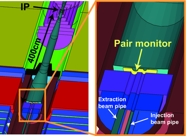
Figure 1: The detector geometry and location of the pair monitor. The pair monitor is located at 400 cm from IP.

Parameter	Unit
Center of mass energy	GeV	500
Number of particles per bunch	$\times 10^{10}$	2.05
Number of bunches per train		2625
Train repetition	Hz	5
Normalized horizontal emittance at IP	mm-mrad	10
Normalized vertical emittance at IP	mm-mrad	0.04
Horizontal beta function at IP	mm	20
Vertical beta function at IP	mm	0.4
Horizontal beam size at IP	nm	639
Vertical beam size at IP	nm	5.7
Longitudinal beam size at IP	$\mu m$	300
Crossing angle	mrad	14

Table 1: The nominal beam parameters for ILC.

3 The reconstruction method of the beam size

We reconstructed the beam sizes from the hit distribution of the pair backgrounds at the pair monitor. The measurement variables used for the reconstruction were, the shoulder radius of the hit distribution, the number of hits in two regions of pair monitor, and the total number of the hits. Since these measurement variables ($m_{i}$, $i=1,2,\cdots,n$) should depend on the beam sizes ($\sigma_{x},\sigma_{y},\sigma_{z}$), they can be expanded around the nominal beam sizes ($\sigma_{x}^{0},\sigma_{y}^{0},\sigma_{z}^{0}$) by the Taylor expansion as follows.

$$\Delta m_{i} = m_{i}(\sigma_{x},\sigma_{y},\sigma_{z})-m_{i}(\sigma_{x}^{0},\sigma_{y}^{0},\sigma_{z}^{0})$$ (2)

$$= \sum_{\alpha=x,y,z}\frac{\partial m_{i}}{\partial\sigma_{\alpha}}\Delta\sigma_{\alpha}+\sum_{\alpha=x,y,z}\sum_{\beta=x,y,z}\frac{1}{2}\Delta\sigma_{\beta}\frac{\partial^{2}m_{i}}{\partial\sigma_{\alpha}\partial\sigma_{\beta}}\Delta\sigma_{\alpha}+\cdots$$

$$= \sum_{\alpha=x,y,z}\left[\frac{\partial m_{i}}{\partial\sigma_{\alpha}}+\frac{1}{2}\sum_{\beta=x,y,z}\Delta\sigma_{\beta}\frac{\partial^{2}m_{i}}{\partial\sigma_{\alpha}\partial\sigma_{\beta}}+\cdots\right]\cdot\Delta\sigma_{\alpha},$$

where $\Delta m_{i}=m_{i}(\sigma_{x},\sigma_{y},\sigma_{z})-m_{i}(\sigma_{x}^{0},\sigma_{y}^{0},\sigma_{z}^{0}),\Delta\sigma_{\alpha}=\sigma_{\alpha}-\sigma_{\alpha}^{0}$. Equation (2) can be expressed by using vectors and matrixes as

$$\Delta\vec{m}=\left[A_{1}+\Delta\vec{\sigma}^{T}\cdot A_{2}+\cdots\right]\cdot\Delta\vec{\sigma},$$ (3)

where $\Delta\vec{m}=(\Delta m_{1},\Delta m_{2},\cdots,\Delta m_{n}),\Delta\vec{\sigma}=(\Delta\sigma_{x},\Delta\sigma_{y},\Delta\sigma_{z})$ and $A_{1}$ is a $n\times 3$ matrix of the first order coefficients of the Taylor expansion and $A_{2}$ is a tensor of the second derivative coefficients. The beam size is reconstructed by multiplying the inverted matrix of a coefficient of $\Delta\vec{\sigma}$ in Equation (3) as follows.

$$\Delta\vec{\sigma}=\left[A_{1}+\Delta\vec{\sigma}^{T}\cdot A_{2}+\cdots\right]^{+}\cdot\Delta\vec{m},$$ (4)

where the superscript “+” indicates the Moore Penrose inversion which gives the inverse matrix of a non-square matrix $A$ as $A^{+}=(A^{T}A)^{-1}A^{T}$ [8, 9].

4 The measurement variables

The maximum radius of hit reflects the maximum transverse momentum of the pairs, which in turn is given by the electromagnetic fields of the oncoming beam. Since the vertical beam size is much smaller than the horizontal and longitudinal beam sizes, the maximum electromagnetic field is inversely proportional to the horizontal and longitudinal beam sizes. Its dependence on the vertical beam size is negligible for the ILC beam condition [3]. Figure 2 shows the radial hit distribution for the nominal beam bunch crossing which shows a shoulder around 8.6 cm which corresponds to the maximum transverse momentum. When the horizontal and/or longitudinal beam size is larger than the nominal beam size, the position of the shoulder is shifted to a smaller radius. We defined the shoulder radius ($R_{shl}$) as the radius to contain 99.8% of all the hits. $R_{shl}$ for the nominal beam sizes is shown by the arrow in Figure 2. Figure 3 shows $R_{shl}$ as a function of the horizontal beam size. As expected, $R_{shl}$ decreases for larger horizontal beam size, and it is almost independent of the vertical beam size. In addition, $R_{shl}$ becomes smaller than that of nominal beam crossing for larger longitudinal beam size.

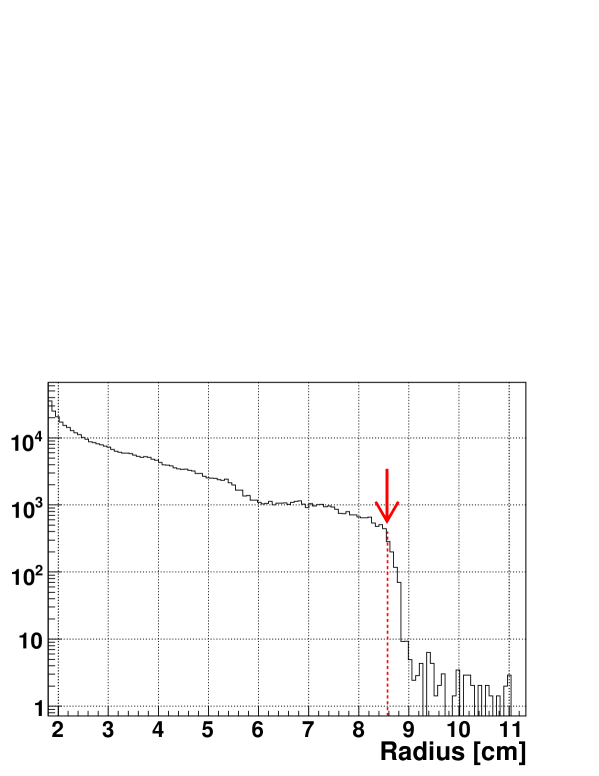
Figure 2: Radial distribution on the pair monitor. The shoulder radius, $R_{shl}$ is defined as the radius to contain 99.8% of all the hits, which is shown as an arrow.

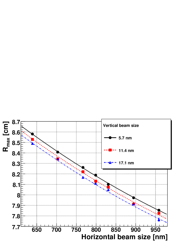
Figure 3: $R_{shl}$ vs. $\sigma_{x}$ fitted with second order polynomials. $R_{shl}$ decreases for larger $\sigma_{x}$ independent of $\sigma_{y}$.

The azimuthal scattering angle of the pairs at the bunch crossing would depend on the horizontal to vertical aspect ratio of the bunch, which would then affect the azimuthal distribution of the hit density on the pair monitor. We thus studied the distribution of the hit density as a function of the radius from the center of the extraction beam pipe ($R$) and the angle around the extraction beam pipe ($\phi$). Figure 4 shows the hit distribution on the pair monitor, and Figure 5 shows the azimuthal hit distribution for $R>0.5\cdot R_{shl}$. A valley at $\phi=$ 0 radian is due to a hole on the pair monitor for the incoming beam around $R\sim 5.6$ cm and $\phi\sim 0$ radian. The shape of the azimuthal hit distribution depends on the radius of the hit distribution around the extraction beam pipe. For example, the radius of the right side in Figure 4 is larger than that of the left side. For that reason, we have more events at $\phi\sim 0$ in Figure 5. We define $N_{0}$ as the number of hits in $-\pi<\phi<-1.2$ radian and $2.7<\phi<\pi$ radian for $R>0.5\cdot R_{shl}$. In order to derive the beam information from the azimuthal distribution, we compared $N_{0}$ to the total number of hits ($N_{all}$). Figure 6 shows $N_{0}/N_{all}$ as a function of the vertical beam size for different horizontal beam sizes. From this result, $N_{0}/N_{all}$ is seen to have information on the horizontal and vertical beam sizes. This ratio is found to be mostly independent of the longitudinal beam size.

In addition, we also use the number of hits $N_{1}$ in $-1.2<\phi<1.8$ radian for $R>0.5\cdot R_{shl}$ to increase the sensitivity to the longitudinal beam size. The ratio $N_{1}/N_{all}$ increases for a larger longitudinal beam size, while it decreases for larger horizontal and vertical beam sizes.

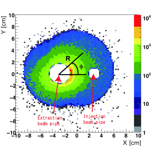
Figure 4: The hit distribution on the pair monitor. There are two holes for the incoming and outgoing beams. The radius(R) and the azimuthal angle are defined as shown in this figure.

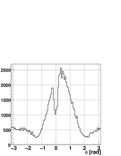
Figure 5: The Azimuthal hit distribution for $R>0.5\cdot R_{shl}$. The valley at 0 radian is caused by a hole for the incoming beam.

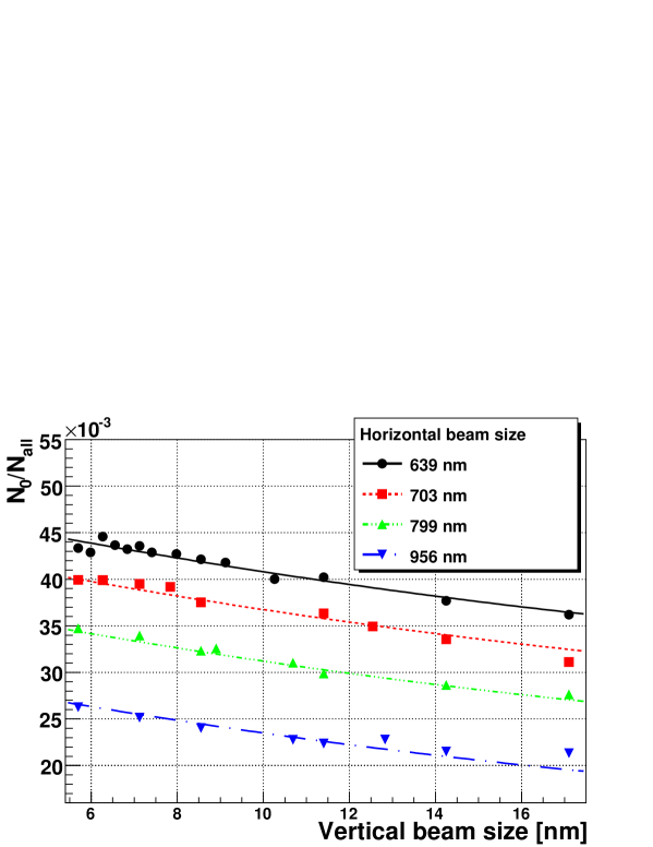
Figure 6: $N_{0}/N_{all}$ vs. $\sigma_{y}$ fitted with second order polynomials, where $N_{0}$ is the number of hits in the region defined by $-\pi<\phi<-1.2$ radian and $2.7<\phi<\pi$ radian for $0.5R_{shl}<R$. $N_{0}/N_{all}$ decreases for larger vertical beam size.

The total number of the hits on the pair monitor, $N_{all}$, reflects the luminosity which is inversely proportional to the vertical and horizontal beam size as shown in Equation (1) [2]. Since the total number of the pair backgrounds are nearly proportional to luminosity, the number of all the hits on the pair monitor is expected to be inversely proportional to the vertical and horizontal beam sizes. Figure 7 shows $1/N_{all}$ as a function of the vertical beam size for several horizontal beam sizes.

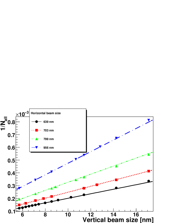
Figure 7: $1/N_{all}$ vs. $\sigma_{y}$ fitted with second order polynomials. $1/N_{all}$ is inversely proportional to the vertical beam size.

5 Reconstruction of beam sizes

To reconstruct the beam sizes, four measurement variables ($R_{shl}$, $N_{0}/N_{all}$, $N_{1}/N_{all}$, $1/N_{all}$) were used in this analysis. Table 2 shows the result of fitting each measurement variable($m_{i}$) with second order polynomials given by

$$m_{i} = m_{i}(\sigma_{x}^{0},\sigma_{y}^{0},\sigma_{z}^{0})+\sum_{\alpha=x,y,z}\frac{\partial m_{i}}{\partial\sigma_{\alpha}}\cdot\sigma_{\alpha}^{0}\cdot\frac{\sigma_{\alpha}-\sigma_{\alpha}^{0}}{\sigma_{\alpha}^{0}}$$ (5)

$$+ \frac{1}{2}\sum_{\alpha=x,y,z}\sum_{\beta=x,y,z}\frac{\partial^{2}m_{i}}{\partial\sigma_{\alpha}\partial\sigma_{\beta}}\cdot\sigma_{\alpha}^{0}\sigma_{\beta}^{0}\cdot\frac{\sigma_{\alpha}-\sigma_{\alpha}^{0}}{\sigma_{\alpha}^{0}}\cdot\frac{\sigma_{\beta}-\sigma_{\beta}^{0}}{\sigma_{\beta}^{0}},$$

where $m_{i}=R_{shl},\ N_{0}/N_{all},\ N_{1}/N_{all},\ 1/N_{all}$. Each measurement variable in the table is normalized by its value for the nominal beam sizes; namely, 8.58, 4.43$\times 10^{-2}$, 1.62$\times 10^{-1}$, and 1.24$\times 10^{-4}$ for $R_{shl}$, $N_{0}/N_{all}$, $N_{1}/N_{all}$, and $N_{all}^{-1}$, respectively. We obtain the numerical values of the matrix ($A_{1}$) and the tensor ($A_{2}$) of Equation (4) by fitting the data by second order polynomials. Then, they were substituted for Equation (3) as follows:

$$\left(\begin{array}[]{l}w_{1}\cdot\Delta R_{shl}\\ w_{2}\cdot\Delta N_{0}/N_{all}\\ w_{3}\cdot\Delta N_{1}/N_{all}\\ w_{4}\cdot\Delta N_{all}^{-1}\end{array}\right) = \left(\begin{array}[]{ccc}w_{1}\cdot\frac{\partial R_{shl}}{\partial\sigma_{x}}&w_{1}\cdot\frac{\partial R_{shl}}{\partial\sigma_{y}}&w_{1}\cdot\frac{\partial R_{shl}}{\partial\sigma_{z}}\\ w_{2}\cdot\frac{\partial N_{0}/N_{all}}{\partial\sigma_{x}}&w_{2}\cdot\frac{\partial N_{0}/N_{all}}{\partial\sigma_{y}}&w_{2}\cdot\frac{\partial N_{0}/N_{all}}{\partial\sigma_{z}}\\ w_{3}\cdot\frac{\partial N_{1}/N_{all}}{\partial\sigma_{x}}&w_{3}\cdot\frac{\partial N_{1}/N_{all}}{\partial\sigma_{y}}&w_{3}\cdot\frac{\partial N_{1}/N_{all}}{\partial\sigma_{z}}\\ w_{4}\cdot\frac{\partial N^{-1}_{all}}{\partial\sigma_{x}}&w_{4}\cdot\frac{\partial N^{-1}_{all}}{\partial\sigma_{y}}&w_{4}\cdot\frac{\partial N^{-1}_{all}}{\partial\sigma_{z}}\\ \end{array}\right)\cdot\left(\begin{array}[]{c}\Delta\sigma_{x}\\ \Delta\sigma_{y}\\ \Delta\sigma_{z}\end{array}\right)$$ (17)

$$+ \left(\begin{array}[]{c}\Delta\sigma_{x}\\ \Delta\sigma_{y}\\ \Delta\sigma_{z}\end{array}\right)^{T}\cdot\biggl{(}\mathrm{O}(2)\biggr{)}\cdot\left(\begin{array}[]{c}\Delta\sigma_{x}\\ \Delta\sigma_{y}\\ \Delta\sigma_{z}\end{array}\right).$$ (24)

The normalization of each measurement variable ($w_{1},w_{2},w_{3},w_{4}$) was adjusted to make the measurement errors of all the variables numerically equal, namely,

$$w_{1}\cdot\Delta R_{shl}=w_{2}\cdot\Delta N_{0}/N_{all}=w_{3}\cdot\Delta N_{1}/N_{all}=w_{4}\cdot\Delta N_{all}^{-1}.$$ (25)

This adjustive method is the same as the method of least squares if there is no correlation between each measurement variable. The beam size at IP is then reconstructed by the inverse matrix method. Since we used second order polynomials for the fitting, we considered up to the second order in Equation (4):

$$\Delta\vec{\sigma}=(A_{1}+\Delta\vec{\sigma}^{T}\cdot A_{2})^{+}\cdot\Delta\vec{m}.$$ (26)

This equation is solved iteratively as follows [9]:

(0)

$\Delta\vec{\sigma}_{0}=A_{1}^{+}\cdot\Delta\vec{m}$

(1)

$\Delta\vec{\sigma}_{1}=\left[A_{1}+\Delta\vec{\sigma}_{0}^{T}A_{2}\right]^{+}\cdot\Delta\vec{m}$
$\vdots$

(n)

$\Delta\vec{\sigma}_{n}=\left[A_{1}+\Delta\vec{\sigma}_{n-1}^{T}A_{2}\right]^{+}\cdot\Delta\vec{m}$

The iteration was repeated until consecutive iterations satisfied

$$\left(\Delta\vec{\sigma}_{n}-\Delta\vec{\sigma}_{n-1}\right)/\Delta\vec{\sigma}_{n}<1\%.$$

Usually, the number of iteration was 3 to 15.

	$R_{shl}$	$N_{0}/N_{all}$	$N_{1}/N_{all}$	$N_{all}^{-1}$
$m_{i}(\sigma_{x}^{0},\sigma_{y}^{0},\sigma_{z}^{0})$	1	1	1	1
$\sigma_{x}^{0}\cdot\partial m_{i}/\partial\sigma_{x}$	-0.20	-1.0	-0.078	1.8
$\sigma_{y}^{0}\cdot\partial m_{i}/\partial\sigma_{y}$	-0.0057	-0.11	-0.0019	0.82
$\sigma_{z}^{0}\cdot\partial m_{i}/\partial\sigma_{z}$	-0.27	-0.0075	0.47	0.54
$\sigma_{x}^{0\ 2}\cdot\partial^{2}m_{i}/\partial\sigma_{x}^{2}$	0.13	0.78	0.083	2.9
$\sigma_{y}^{0\ 2}\cdot\partial^{2}m_{i}/\partial\sigma_{y}^{2}$	0.00085	0.022	-0.012	-0.0011
$\sigma_{z}^{0\ 2}\cdot\partial^{2}m_{i}/\partial\sigma_{z}^{2}$	0.21	-0.48	-0.31	0.26
$2\sigma_{x}^{0}\sigma_{y}^{0}\cdot\partial^{2}m_{i}/\partial\sigma_{x}\partial\sigma_{y}$	0.00015	0.0090	-0.011	1.3
$2\sigma_{y}^{0}\sigma_{z}^{0}\cdot\partial^{2}m_{i}/\partial\sigma_{y}\partial\sigma_{z}$	0.0017	0.026	0.0072	0.35
$2\sigma_{z}^{0}\sigma_{x}^{0}\cdot\partial^{2}m_{i}/\partial\sigma_{z}\partial\sigma_{x}$	0.039	-0.014	0.019	1.4

Table 2: Result of fitting each measurement variable with second order polynomials as given by Equation (5).

Figure 8 shows the relative deviations of the horizontal, vertical, and longitudinal beam sizes for 50 bunch crossings. The errors for the distribution of these deviations are estimated at 5.1%, 10.0%, and 4.0% for the horizontal, vertical, and longitudinal beam sizes, respectively. Then, we conclude that the pair monitor can measure the beam sizes with accuracies of 5.1% (33 nm), 10.0% (0.57 nm), and 4.0% (12 $\mu$m) for the horizontal, vertical, and longitudinal beam sizes, respectively.

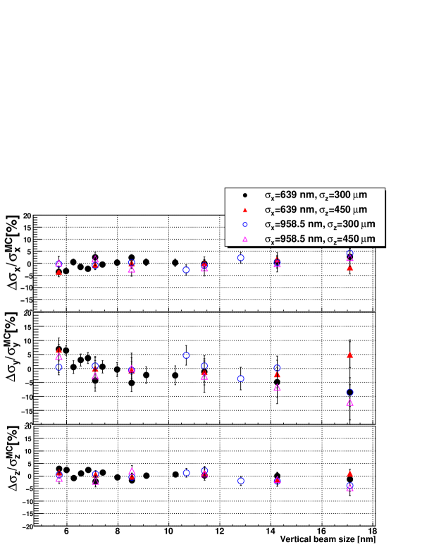
Figure 8: Relative deviations of, from the top, horizontal, vertical and longitudinal beam sizes.

6 Conclusions

We studied a technique of beam size measurement with the pair monitor. The method utilizes the second order inversion of the Taylor expansion. Four measurement variables ($R_{shl}$, $N_{0}/N_{all}$, $N_{1}/N_{all}$ and $1/N_{all}$) were used to reconstruct the beam sizes, and the matrix elements of the expansion were obtained by fitting with second order polynomials of the beam sizes. The measurement accuracies of the horizontal, vertical, and longitudinal beam sizes were found to be 5.1%, 10.0%, and 4.0%, respectively, for 50 bunch crossings. This result confirms that the pair monitor has, at least statistically, enough sensitivity to measure the beam size at IP for ILC.

References

- [1] ILC Global Design Effort and World Wide Study, International linear collider Reference Design Report (2007).
- [2] D. Schulte, Study of Electromagnetic and Hadronic Background in the Interaction Region of the TESLA Collider (1996).
- [3] T. Tauchi and K. Yokoya, Nanometer Beam-Size Measurement during Collisions at Linear Colliders, KEK preprint 94-122.
- [4] T. Tauchi, K. Yokoya and P. Chen, Pair creation from beam-beam interaction in linear colliders, Particle Accelerator 41, 29 (1993).
-
[5]
Y. Takubo, Proceedings of LCWS 2007,
http://www-zeuthen.desy.de/ILC/lcws07/pdf/MDI/takubo_yosuke.pdf -
[6]
Jupiter web-page:
http://acfahep.kek.jp/subg/sim/simtools/ -
[7]
CAIN web-page:
http://lcdev.kek.jp/~yokoya/CAIN/cain235/ - [8] A. Stahl, Diagnostics of Colliding Bunches from Pair Production and Beam-Strahlung at the IP, LC-DET-2005-003.
- [9] M. Ternick, Fast Beam Diagnostics through Beamstrahlung at TESLA.
-
[10]
FCAL collaboration web-page:
http://www-zeuthen.desy.de/ILC/fcal/