Interactions of massless monopole clouds

Abstract

Some spontaneously broken gauge theories with unbroken non-Abelian gauge groups contain massless magnetic monopoles that are realized classically as clouds of non-Abelian field surrounding one or more massive monopoles. We use moduli space methods to investigate the properties of these massless monopole clouds. We show that the natural metric on the Nahm data for a class of SU($2M+2$) solutions with $2M$ massive and $M(2M-1)$ massless monopoles can be obtained from that for a simpler class of SU($M+1$) solutions. For the $M=1$ case, we show that the Nahm data metric is isomorphic to the metric for the moduli of the BPS solutions, thus verifying a previously conjectured result. For $M=2$ we use our results and the moduli space approximation to obtain an effective Lagrangian for an axially symmetric class of solutions. Using this Lagrangian, we study the interactions between the two types of clouds that appear. We show that, although the static spacetime field configurations suggest that the clouds might be rather diffuse, in scattering processes they behave as if they were relatively thin hard shells.

I Introduction

$N=4$ supersymmetric Yang-Mills theory is believed to possess an electric-magnetic duality symmetry. When the gauge group is maximally broken, to an Abelian subgroup, this duality interchanges the massive electrically charged particles corresponding to the elementary fields with magnetically charged states arising from classical soliton solutions. If the unbroken symmetry has a non-Abelian component, then there exist massless particles carrying electric-type charge. Although there are no isolated massless solitons, certain multisoliton solutions have degrees of freedom that are naturally interpreted as corresponding to massless magnetic monopoles. These are manifested as clouds of non-Abelian field that surround one or more massive monopoles and shield part of their non-Abelian magnetic charge Lee:1996vz . Our aim in this paper will be to explore the properties of these massless monopoles by studying the interactions between these clouds.

To explain this in more detail, consider an SU($N$) gauge theory with an adjoint Higgs field whose asymptotic value can be brought into the form

$$\Phi={\rm diag}\,(s_{1},s_{2},\dots s_{N})$$ (1)

with $s_{1}\leq s_{2}\leq\dots s_{N}$. If the $s_{i}$ are all distinct, the gauge symmetry is broken maximally, to U(1)^N-1, and there are $N-1$ topological charges. If the asymptotic magnetic field is then written in the form $F_{ij}=\epsilon_{ijk}r_{k}\,Q_{M}/r^{3}$, with

$$Q_{M}={\rm diag}\,(n_{1},n_{2}-n_{1},\dots,-n_{N-1})\,,$$ (2)

these topological charges are the $n_{k}$. We will refer to an SU($N$) monopole solution with such charges as being an $(n_{1},n_{2},\dots,n_{N-1})$ solution.

With this maximal symmetry breaking, one can identify $N-1$ fundamental monopoles Weinberg:1979zt , each carrying a single unit of one of the topological charges, with the mass of the $k$th being $(4\pi/e)(s_{k+1}-s_{k})$. Each of these has four degrees of freedom — three position variables and one U(1) phase. A BPS solution with arbitrary magnetic charges can be understood as being composed of appropriate numbers of the various species of fundamental monopoles and as living on a moduli space whose dimension is four times the total number of component monopoles.

Our interest here is not in maximal gauge symmetry breaking, but rather in the alternative possibility, where $\Phi$ has degenerate eigenvalues. The unbroken symmetry is then enhanced to a non-Abelian group, and some of the fundamental monopoles become massless. It is instructive to follow the behavior of the classical solutions as this case is obtained from the maximally broken one by smoothly varying the eigenvalues of $\Phi$. One finds that an isolated fundamental monopole solution goes over to the vacuum solution as it becomes massless. The behavior of multimonopole solutions is more complex Lu:1998br . If the total magnetic charge remains purely Abelian, then the solution rapidly approaches its limiting form once the inverse of the smallest monopole mass becomes larger than the separations of the component monopoles. In addition, the moduli space of solutions and its naturally defined metric have smooth limits; in the examples where the metric for the case with nonmaximal breaking has been found directly, it is indeed the limit of the metric for the maximally broken case Lee:1996vz ; Houghton:1999qu .

If instead the magnetic charge has a non-Abelian component, none of these are the case. Not only do the moduli spaces not have smooth limits, but cases that are gauge equivalent in the massless limit have different dimensions for any finite monopole mass. These pathologies are clearly related to the long-range behavior of the non-Abelian fields and the non-normalizability of certain zero modes in the massless limit. A simple example of this arises in an SU(3) gauge theory. With maximal breaking, the unbroken symmetry is U(1)$\times$U(1), and there are two species of fundamental monopoles. If two of the eigenvalues of $\Phi$ are equal, the unbroken symmetry is SU(2)$\times$U(1) and one of the fundamental monopoles is massless. In the maximally broken case, the moduli spaces of the (2,0) and the (2,2) solutions have dimensions four and twelve, respectively. Yet, when the breaking is nonmaximal an SU(2) gauge transformation can turn a (2,[0]) solution into a (2,[2]) solution, where the square brackets denote the massless species. On the other hand, the (2,[1]) solutions, which have a purely Abelian long-range field have a well-defined moduli space, with a metric that is a smooth limit of the (2,1) metric.

In this paper we will restrict ourselves to configuration with purely Abelian magnetic charge. Several such solutions with a single massless monopole are known. These include solutions Weinberg:1982jh with one massive and one massless monopole for SO(5) broken to SU(2)$\times$U(1), as well as SU(4) (1,[1],1) solutions Weinberg:1998hn and the SU(3) (2,[1]) solutions Dancer:1992kj referred to above, each with one massless and two massive monopoles. These SU(3) solutions will be of particular importance in our analysis. Their properties were studied in considerable detail by Dancer and collaborators Dancer:1992kj ; Dancer:1992kn ; Dancer:1992hf ; Dancer:1997zx , and we will refer to them, and their $(N-1,[N-2],\dots,[1])$ generalizations for SU($N$), as Dancer solutions.

In all of these solutions there is a single non-Abelian cloud (spherical in the first case, ellipsoidal in the latter two) that encloses the massive monopole(s). Well inside this cloud, the magnetic field approximates the field, with both Abelian and non-Abelian magnetic components, that would be expected to arise just from the massive monopoles. The cloud effectively shields the non-Abelian components, so that outside the cloud one sees the purely Abelian field corresponding to the sum of the massive and massless monopole charges. The size of the cloud is determined by a single parameter, whose value has no effect on the total energy of the solution.

Since our goal in this paper is to investigate the interaction between massless monopole clouds, we need solutions that have more than one cloud. One might have expected that these could be obtained simply by having more than one massless monopole. This turns out not to be so. For example, the SU($N$) (1,[1],…,[1],1) solutions contain $N-3$ massless monopoles, but only a single cloud, no matter how large $N$ becomes Lee:1996vz . [In fact, for $N>4$ these solutions are essentially embeddings of (1,[1],1) SU(4) solutions into the larger group.]

A set of solutions that do have multiple clouds, and which we will focus on, are the (2,[2],[2],[2],2) solutions — with four massive and six massless monopoles — in the theory with SU(6) broken to U(1)$\times$SU(4)$\times$U(1). The structure of these solutions was studied in Ref. Houghton:2002bz . They can be viewed as containing two SU(3) Dancer solutions, each with a “Dancer cloud” enclosing two massive monopoles, embedded in disjoint subgroups of the SU(6). In addition, there are two larger “SU(4) clouds”, enclosing both Dancer clouds, that are somewhat analogous to the cloud in the SU(4) (1,[1],1) solutions. As we will describe in more detail later, these four clouds are characterized not only by individual cloud-size parameters, but also by a number of additional parameters specifying their orientations with respect to the unbroken gauge group. Note that, even in this case, the number of clouds is less than the number of massless monopoles.

A useful tool for studying the low-energy dynamics of multimonopole systems such as these is the moduli space approximation Manton:1981mp , which reduces the full field theory dynamics to that of a finite number of collective coordinates $z^{a}$. The latter are governed by the Lagrangian

$$L={1\over 2}g_{ab}\dot{z}^{a}\dot{z}^{b}\,,$$ (3)

where $g_{ab}$ is the metric on the moduli space of BPS solutions. This method was used to study the (1,[1],1) SU(4) solutions Chen:2001ge . Because the two massive monopoles lie in mutually commuting subgroups of the SU($4$), one would not expect them to interact directly with each other. This turns out to be the case; indeed, they can pass though each other undeflected. On the other hand, they do interact with, and exchange energy with, the cloud. In these interactions the cloud acts as if it were a thin shell, with the monopole-cloud interactions concentrated in the times when the massive monopole positions coincide with the shell. At large times the massive monopoles and the cloud decouple from each other and evolve independently. The interactions between the cloud and the massless monopoles are similar in the SU(3) Dancer solutions Dancer:1992kn ; Dancer:1992hf , which have the additional feature that the massive monopoles, being both of the same type, also interact directly with each other.

A word of caution is in order here. The essential idea underlying the moduli space approximation is that for a slowly moving soliton fluctuations off of the moduli space are energetically suppressed. If the theory contains massless particles, this needs further examination, since excitation of these modes by radiation of massless particles is always energetically possible. However, since the source of the radiation is proportional to the time derivative of the bosonic fields, the radiation rate is expected to be small for low soliton velocities. This has been shown rigorously for configurations involving pairs of monopoles in theories where the massless gauge fields are all Abelian Manton:1988bn ; Stuart:1994tc . Although the validity of the approximation has not been demonstrated rigorously for the case where there are massless non-Abelian gauge fields, explicit comparison of the predictions of the moduli space approximation with numerical evolution of the full field equations in a spherically symmetric example Chen:2001qt show that they agree as long as the configurations are slowly varying.

Of course, this method requires that moduli space metric be known. It can be obtained directly from the BPS solutions, if they are known explicitly. In some other cases indirect methods based on the mathematical properties of the moduli space can be used to obtain $g_{ab}$ Atiyah:1985dv ; Lee:1996if ; Gauntlett:1996cw . However, for other cases it turns out to be easiest to resort to an alternative approach. The Atiyah-Drinfeld-Hitchin-Manin-Nahm (ADHMN) construction Nahm:1982jb ; Nahm:1981xg ; Nahm:1981nb ; Nahm:1983sv is a powerful tool for obtaining BPS solutions. It is based on an equivalence between the Bogomolny equation for the fields in three-dimensional space and an ordinary differential equation for a set of matrix functions of a single variable, known as the Nahm data. The moduli space of Nahm data has its own naturally defined metric. It has been shown for both the SU(2) theory nakajima and for the case of SU($N+1$) broken to U($N$) takahasi , and is believed to be true in general, that the moduli spaces of Nahm data and of BPS solutions are isometric. [In particular, Dancer used this equivalence in his investigation of the dynamics of the SU(3) solutions, and worked with the Nahm data metric.] In this paper we will assume that the equivalence of the two metrics holds as well for our SU(6) example, and will work with the Nahm data metric.

The remainder of this paper is organized as follows. In Sec. II we review the relevant parts of the ADHMN construction, as well as the metric on the moduli space of Nahm data. We then show that if the metric for the SU($M+1$) Dancer solutions is known, then that for the $(M,[M],\dots,[M],M)$ solutions of SU($2M+2$) broken to U(1)$\times$SU($2M$)$\times$U(1) can be easily obtained. In Sec. III we illustrate this method by obtaining the metric for the (1,[1],1) SU(4) solutions and verify that the Nahm data metric thus obtained is in fact equivalent to the metric on the moduli space of BPS solutions, which had been found previously Lee:1996vz ; Chen:2001ge ; Lee:1996kz . Next, in Sec. IV, we turn to the moduli space metric for the SU(6) (2,[2],[2],[2],2) solutions. These are described by a total of 40 collective coordinates. Although the full metric can be obtained by the methods of Sec. II, the result would be rather unwieldy for exploring the nature of the cloud dynamics. We therefore consider a restricted problem, that of a lower-dimensional submanifold of axially symmetric solutions, for which the metric has a relatively simple closed form expression but which still has enough structure to allow us to investigate nontrivial cloud dynamics. In Sec. V we use the metric obtained in the previous section to explore the cloud-cloud interactions. Section VI contains some concluding remarks. There is an Appendix, which contains some of the details of the moduli space metric calculation.

II The ADHMN construction and the metric for $\bm{(M,[M],\dots,[M],M)}$ solutions

As was discussed in Sec. I, the moduli spaces of BPS solutions and of Nahm data are believed to be isometric. We work in this paper with the Nahm data metric, which is the more accessible of the two for the examples that we study. In this section we first review the essential elements of the ADHMN construction Nahm:1982jb ; Nahm:1981xg ; Nahm:1981nb ; Nahm:1983sv , emphasizing the points that are relevant for the $(M,[M],\dots,M)$ solutions of SU($2M+2$). We then obtain a general expression for the metric of these SU($2M+2$) solutions, and briefly discuss an asymptotic special case.

II.1 Nahm data

The basic elements in the ADHMN construction are the Nahm data, a quadruple of matrix functions $T_{\mu}(s)$ ($\mu=0,1,2,3$) that obey the Nahm equation,

$$0={dT_{i}\over ds}+i[T_{0},T_{i}]+{i\over 2}\epsilon_{ijk}[T_{j},T_{k}]\,,\qquad i,j,k=1,2,3\,.$$ (1)

For charge $k$ solutions in an SU(2) theory with Higgs vacuum expectation value $v$, the $T_{\mu}(s)$ are $k\times k$ Hermitian matrices defined for $-v/2\leq s\leq v/2$. For a general SU($N$) theory, the eigenvalues of the Higgs vacuum expectation value divide the range of $s$ into $N-1$ intervals, on each of which Eq. (1) must hold. (The boundary conditions at the ends of these intervals are somewhat involved; we describe them below for the cases we need.) The dimension of the $T_{\mu}$ varies from interval to interval, being determined on each by the corresponding magnetic charge. If the $T_{\mu}$ are of the same size, $k\times k$, on two adjacent intervals, then there are additional “jumping data”, forming a $2k$-component complex vector, associated with the boundary between these intervals.

For later reference, note that if the $T_{\mu}(s)$ satisfy the Nahm equation, then so do the $\tilde{T}_{\mu}$ defined by

$$\tilde{T}_{i}(s) = R_{ij}T_{j}(s)+B_{i}\,,$$ (2)

$$\tilde{T}_{0}(s) = T_{0}(s)\,,$$ (3)

where $R_{ij}$ is an orthogonal matrix with determinant one. The $\tilde{T}_{\mu}(s)$ lead to a spacetime solution that is obtained from the original one by a combination of the spatial rotation specified by $R$ and a spatial translation by the vector $\bf B$.

For SU($2M+2$) broken to U(1)$\times$SU($2M$)$\times$U(1) the eigenvalues of the Higgs vacuum expectation value are $s_{L}<s_{0}<s_{R}$, with $s_{0}$ being $2M$-fold degenerate. These divide the range of $s$ into a “left” interval $[s_{L},s_{0}]$, a “right” interval $[s_{0},s_{R}]$, and $2M-1$ intervals of zero width at $s=s_{0}$. These correspond to two species of massive monopoles, with masses

$$M_{L}=4\pi(s_{0}-s_{L})\,,\qquad M_{R}=4\pi(s_{R}-s_{0})\,,$$ (4)

and $2M-1$ species of massless fundamental monopoles. For the $(M,[M],\dots,[M],M)$ solutions we need two sets of $M\times M$ matrices, $T_{\mu}^{L}(s)$ and $T_{\mu}^{R}(s)$, defined on the left and right intervals, respectively. These obey Eq. (1) subject to the boundary condition that, for $M>1$, the $T_{i}^{L}$ ($T_{i}^{R}$) have poles at $s_{L}$ ($s_{R}$) with the residues forming an $M$-dimensional irreducible representation of SU(2). Except for these poles, the $T_{\mu}^{L}$ and $T_{\mu}^{R}$ must be everywhere nonsingular.

Because the magnetic charge is the same on adjacent intervals, there are jump data associated with each of the $2M$ coincident boundaries at $s_{0}$. We write the data associated with the $F$th boundary as a $2M$-component vector $a_{\alpha r}^{F}$, where $r=1,2,\dots,M$ and $\alpha=1,2$. These jump data are required to satisfy the constraint

$$\left(\Delta T_{j}\right)_{rs}=\left[T_{j}^{L}(s_{0})\right]_{rs}-\left[T_{j}^{R}(s_{0})\right]_{rs}={1\over 2}\sum_{F\alpha\beta}a_{\alpha s}^{F*}(\sigma_{j})_{\alpha\beta}a_{\beta r}^{F}\,.$$ (5)

If we assemble the jump data into a $2M\times 2M$ matrix $A$ with $A_{\alpha r,F}=a_{\alpha r}^{F}$, and define an $M\times M$ matrix

$$(T_{4})_{rs}={1\over 2}\sum_{F\alpha}a_{\alpha s}^{F*}a_{\alpha r}^{F}$$ (6)

and a $2M\times 2M$ matrix

$$K_{\alpha r;\beta s}\equiv(\Delta T_{j})_{rs}(\sigma_{j})_{\alpha\beta}+(T_{4})_{rs}\delta_{\alpha\beta}=\sum_{F}a_{\beta s}^{F*}a_{\alpha r}^{F}\,,$$ (7)

the jump data constraint becomes simply $K=AA^{\dagger}$. For later reference, it is important to note that this implies that the eigenvalues of $K$ must be positive. The general solution of this constraint is

$$A=K^{1/2}V\,,$$ (8)

where $V$ is unitary. The freedom in the choice of $V$ reflects the existence of an unbroken U(1)$\times$SU($2M$) subgroup of the original SU($2M+2$) gauge group.

The crucial observation for us is that the dimensions and boundary conditions for the $T_{\mu}^{L}$ and $T_{\mu}^{R}$ are the same as those for the Nahm data of the SU($M+1$) Dancer solution. Apart from the gauge orientation angles and phases encoded in $V$, the new information specific to the SU($2M+2$) problem — i.e., the parameters that describe the SU($2M$) clouds — enters only through $T_{4}$, which can be chosen to be any Hermitian matrix, subject only to the constraint that the eigenvalues of $K$ must be positive. Thus, if the Nahm equation has already been solved for the SU($M+1$) Dancer problem, the only additional data needed for the $(M,[M],\dots,[M],M)$ solutions are the jump data, which are given by Eq. (8).

II.2 Gauge action

In addition to the spacetime symmetries described by Eq. (3), the Nahm equations have a set of invariances that are analogous to, although distinct from, the gauge transformations on the spacetime fields. If $g(s)$ is a unitary matrix of appropriate dimension, the Nahm equation (1) and the jump equation (5) are invariant under

$$T_{\mu}(s) \rightarrow \tilde{T}_{\mu}(s)=g(s)T_{\mu}(s)g^{-1}(s)+i\delta_{\mu 0}{dg\over ds}g^{-1}(s)\,,$$ (9)

$$A_{\alpha r,F} \rightarrow \tilde{A}_{\alpha r,F}=g(s_{0})_{rs}A_{\alpha s,F}\,.$$ (11)

When considering spacetime gauge transformations one distinguishes between local gauge transformations, which approach the identity at spatial infinity, and global gauge transformations, which are nontrivial as $r\rightarrow\infty$. While the former simply reflect the presence of redundant field components, the latter correspond to symmetries that are related to conserved gauge charges. When the gauge symmetry is unbroken, the number of global gauge transformations is equal to the dimension of the gauge group. If the symmetry is spontaneously broken, as it must be when monopoles are present, only those global gauge transformations that leave the asymptotic Higgs field invariant (i.e., those in the unbroken gauge group) lead to normalizable zero modes about a static solution, and only these correspond to physical motions on the moduli space.

Similarly, we can distinguish between local gauge actions on the Nahm data, for which $g(s)=I$ at both boundaries, and global gauge actions, which have $g\neq I$ at one or both boundaries. Any of the latter that act on pole terms in the Nahm data will lead to nonnormalizable modes, and therefore do not contribute to the moduli space dynamics. This means that for the $(M,[M],\dots,M)$ solutions, which have poles at both boundaries, the only relevant global gauge actions are those that leave the pole terms invariant. These are proportional to the unit matrix and are of the form $g(s)=e^{i\chi(s)}I$. Because an $s$-independent gauge action proportional to the unit matrix would have no effect on the Nahm data, it is sufficient to consider the case where $\chi$ vanishes at one boundary, but not at the other; this leads to a zero mode corresponding to an unbroken U(1). The zero modes corresponding to the other unbroken generators do not arise from gauge actions, but instead correspond to variations of $V$.

For the SU($M+1$) Dancer solutions there must be a pole at one boundary, but the only constraint at the other is that the Nahm data be nonsingular. There are then a total of $M^{2}$ independent normalizable global gauge zero modes, corresponding to the generators of the unbroken U($M$). These can be obtained from gauge actions for which $g$ is an $M$-dimensional unit matrix at the pole and proportional to one of the generators of U($M$) at the other boundary.

II.3 The moduli space metric

The moduli space of Nahm data is the space of solutions of the Nahm and jump equations, but with solutions that are related by local gauge actions considered equivalent. The coordinates on this space are the collective coordinates $z_{a}$. Its tangent space at a given point is spanned by the variations of the Nahm data that preserve the Nahm and jump equations and that are orthogonal to the variations due to local gauge actions.

For our solutions, the Nahm data consist of two quadruples of Nahm matrices, one for each interval, and jump data at the boundary at $s_{0}$. We can write these collectively as ${\cal T}=\{T^{L}_{\mu}(s),T^{R}_{\mu}(s),A\}$. The tangent vectors to the Nahm data moduli space must have a similar structure, and so can be written as ${\cal Y}=\{Y^{L}_{\mu}(s),Y^{R}_{\mu}(s),Y\}$. The inner product of two such vectors is defined to be

$$\langle{\cal Y},{\cal Y^{\prime}}\rangle=\int_{s_{L}}^{s_{0}}\,{\rm Tr\,}Y^{L}_{\mu}(s)Y^{{}^{\prime}L}_{\mu}(s)+\int_{s_{0}}^{s_{R}}\,{\rm Tr\,}Y^{R}_{\mu}(s)Y^{{}^{\prime}R}_{\mu}(s)+{1\over 2}{\rm Tr\,}(YY^{{}^{\prime}\dagger}+Y^{\prime}Y^{\dagger})\,.$$ (12)

An infinitesimal local gauge action is specified by a Hermitian matrix function $\Lambda(s)$ that is everywhere continuous and vanishes at $s_{L}$ and $s_{R}$. We denote its values on the left and right intervals by $\Lambda^{L}(s)$ and $\Lambda^{R}(s)$, and define $\Lambda(s_{0})\equiv\Lambda^{0}$. Its action on the Nahm data defines a vector ${\cal Y}_{\rm gauge}$ with

$$(Y_{\rm gauge})_{\mu}^{L,R} = \delta_{\Lambda}T_{\mu}^{L,R}=\delta_{\mu 0}{d\Lambda^{L,R}\over ds}+i[T_{\mu}^{L,R},\Lambda^{L,R}]\equiv D_{\mu}\Lambda^{L,R}\,,$$ (13)

$$(Y_{\rm gauge})_{\alpha r,F} = (\delta_{\Lambda}A)_{\alpha r,F}=-i\Lambda^{0}_{rs}A_{\alpha s,F}\,,$$ (15)

where $D_{j}=i[T_{j}(s),~{}]$ and $D_{0}=d/ds+i[T_{0}(s),~{}]$. In order that $\cal Y$ be orthogonal to ${\cal Y}_{\rm gauge}$ for any choice of $\Lambda$, we must require that

$$0 = D_{\mu}Y_{\mu}^{L,R}(s)\,,\qquad s\neq s_{0}\,,$$ (16)

$$0 = \left[Y_{0}^{L}(s_{0})-Y_{0}^{R}(s_{0})\right]_{rs}+{i\over 2}(YA^{\dagger}-AY^{\dagger})_{\alpha r,\alpha s}\,.$$ (17)

By analogy with the corresponding constraint on the variations of the spacetime fields, we will refer to these as the background gauge conditions.

A basis for the tangent space is given by a set of vectors ${\cal Y}_{a}$ of the form

$$Y_{a\mu}^{L,R}(s) = {\partial T_{\mu}^{L,R}(s;z)\over\partial z^{a}}+D_{\mu}\Lambda_{a}^{L,R}\,,$$ (18)

$$Y_{a} = {\partial A\over\partial z^{a}}-i[\Lambda_{a}(s_{0})\otimes A]\,,$$ (20)

with the gauge action $\Lambda_{a}(s)$ chosen so that ${\cal Y}_{a}$ is in background gauge. The metric on the moduli space is then defined to be

$$ds^{2}=g_{ab}\,dz^{a}dz^{b}=4\pi\langle{\cal Y}_{a},{\cal Y}_{b}\rangle\,dz^{a}dz^{b}\,.$$ (21)

II.4 The metric for the $\bm{(M,[M],\dots,M)}$ solutions of SU($\bm{2M+2}$)

As we have just seen, to calculate the moduli space metric one must first vary the Nahm data with respect to the coordinates, and then find a gauge action $\Lambda(s)$ that brings the resulting tangent vector into background gauge. The one part of this procedure that is not completely straightforward is the solution of the differential equation for $\Lambda(s)$ that is implied by Eqs. (16) and (20). However, if this has already been done for the SU($M+1$) Dancer solutions, the determination of the moduli space metric for the $(M,[M],\dots,M)$ solutions of SU($2M+2$) reduces to an algebraic problem. To see this, first note that the Dancer problems give us two sets of basis vectors, $Y^{DL}_{a\mu}$ and $Y^{DR}_{a\mu}$, that satisfy Eq. (16) on their respective domains. Each of these sets includes $M^{2}$ vectors corresponding to the global U($M$) gauge freedom. These are of the form $Y^{L}_{f\mu}=D_{\mu}\chi_{f}^{L}$ and $Y^{R}_{f\mu}=D_{\mu}\chi^{R}_{f}$ ($f=1,2,\dots M^{2}$), where $\chi_{f}^{L}$ ($\chi_{f}^{R}$) vanishes at $s_{L}$ ($s_{R}$) and is nonzero and proportional to one of the U($M$) generators at $s_{0}$. Because the Dancer basis vectors satisfy Eq. (16),

$$D_{\mu}D_{\mu}\chi_{f}^{L}=D_{\mu}D_{\mu}\chi_{f}^{R}=0\,.$$ (22)

Now suppose that the coordinates for the $(M,[M],\dots,M)$ solutions are chosen so that one subset are those originating with the left Dancer problem, a second subset are those from the right Dancer problem, and the remainder are associated only with the jump data. The tangent vector corresponding to the coordinate $z^{a}$ can then be written in the form

$${\cal Y}_{a}=\left\{Y_{a\mu}^{DL}+D_{\mu}\Lambda^{L}_{a},Y_{a\mu}^{DR}+D_{\mu}\Lambda^{R}_{a},{\partial A\over\partial z^{a}}-i(\Lambda_{a}^{0}\otimes I_{2})A\right\}\,,$$ (23)

where $Y_{a\mu}^{DL}$ and $Y_{a\mu}^{DR}$ are the vectors from the left and right Dancer problems. Although these Dancer vectors already satisfy the background gauge condition on their respective domains, an additional gauge action may be needed to satisfy Eq. (17) at $s_{0}$. Its gauge function $\Lambda$ must vanish at $s_{L}$ and $s_{R}$ and, in order to maintain the background gauge condition on the two intervals, it must satisfy $D_{\mu}D_{\mu}\Lambda=0$ for $s\neq s_{0}$. It is therefore a linear combination of Dancer global gauge modes, with

$$\Lambda^{L}_{a} = c^{L}_{af}\chi_{f}^{L}\,,$$ (24)

$$\Lambda^{R}_{a} = c^{R}_{af}\chi_{f}^{R}\,.$$ (25)

Thus, for each ${\cal Y}_{a}$ there are a total of $2M^{2}$ constants to be determined. Requiring continuity of the gauge action at the boundary, $\Lambda^{0}_{a}=\Lambda^{L}_{a}(s_{0})=\Lambda^{R}_{a}(s_{0})$, gives $M^{2}$ algebraic equations. The background gauge condition at the boundary becomes

$$\left[D_{0}\Lambda^{L}_{a}(s_{0})-D_{0}\Lambda^{R}_{a}(s_{0})+\Lambda^{0}_{a}T_{4}+T_{4}\Lambda^{0}_{a}\right]_{rs} = \left[Y_{a0}^{DR}(s_{0})-Y_{a0}^{DL}(s_{0})\right]_{rs}$$ (28)

$$\qquad+{i\over 2}\left(A{\partial A^{\dagger}\over\partial z_{a}}-{\partial A\over\partial z_{a}}A^{\dagger}\right)_{\alpha r,\alpha s}$$

and gives $M^{2}$ more equations, thus determining the $c^{L}_{af}$ and $c^{R}_{af}$, and hence ${\cal Y}_{a}$.

We can now evaluate the metric. Because the ${\cal Y}_{a}$ satisfy the background gauge conditions of Eqs. (16) and (17) and, in addition, $D_{\mu}Y_{a\mu}^{DL}=D_{\mu}Y_{a\mu}^{DR}=0$, many of the terms involving the gauge actions can be eliminated by integrations by parts. With the aid of Eq. (28), one eventually obtains

$$g_{ab} = 4\pi\int_{s_{L}}^{s_{0}}ds\,{\rm Tr\,}Y_{a\mu}^{DL}Y_{b\mu}^{DL}+4\pi\int_{s_{0}}^{s_{R}}ds\,{\rm Tr\,}Y_{a\mu}^{DR}Y_{b\mu}^{DR}+g_{ab}^{0}$$ (29)

$$= g_{ab}^{DL}+g_{ab}^{DR}+g_{ab}^{0}\,,$$ (31)

where $g_{ab}^{DL}$ and $g_{ab}^{DR}$ are the metric components from the corresponding Dancer solutions and

$$g_{ab}^{0} = 4\pi\,{\rm Tr\,}\left[Y_{a0}^{DL}(s_{0})-Y_{a0}^{DR}(s_{0})\right]\Lambda^{0}_{b}+2\pi\,{\rm Tr\,}\left({\partial A\over\partial z^{a}}{\partial A^{\dagger}\over\partial z^{b}}+{\partial A\over\partial z^{b}}{\partial A^{\dagger}\over\partial z^{a}}\right)$$ (33)

$$\qquad+2\pi i\,{\rm Tr\,}\left[{\partial A\over\partial z^{a}}A^{\dagger}(\Lambda_{b}^{0}\otimes I_{2})-(\Lambda_{b}^{0}\otimes I_{2})A{\partial A^{\dagger}\over\partial z^{a}}\right]$$

$$= 2\pi\,{\rm Tr\,}\left({\partial A\over\partial z^{a}}{\partial A^{\dagger}\over\partial z^{b}}+{\partial A\over\partial z^{b}}{\partial A^{\dagger}\over\partial z^{a}}\right)+4\pi\,{\rm Tr\,}\left[D_{0}\Lambda^{R}_{a}(s_{0})-D_{0}\Lambda^{L}_{a}(s_{0})\right]\Lambda_{b}^{0}$$ (36)

$$\qquad-4\pi\,{\rm Tr\,}T_{4}\left(\Lambda_{a}^{0}\Lambda_{b}^{0}+\Lambda_{b}^{0}\Lambda_{a}^{0}\right)$$

contains the entire contribution from the jump data. These two equations are the main result of this section.

II.5 Large SU($2M$) clouds

Before focusing on the specific examples of $M=1$ and $M=2$, it is worth commenting briefly on the case where the length scales in $T_{\mu}^{DL}$ and $T_{\mu}^{DR}$ are smaller than all those entering $T_{4}$ by a factor of $\epsilon\ll 1$. This corresponds to the situation where the SU($2M$) clouds are large compared to both the Dancer clouds and the separations between the massive monopoles. In this case Eq. (8) can be written as

$$A=(T_{4}^{1/2}\otimes I_{2})V+\delta A\,,$$ (37)

where $\delta A$, which contains all of the information about the Dancer data, is suppressed by a factor of $\epsilon$. Therefore, if $z_{a}$ is one of the Dancer coordinates, $\partial A/\partial z_{a}=O(\epsilon)$. Furthermore, by noting the $\Lambda_{a}^{0}T_{4}$ terms on the left-hand side of Eq. (28), we see that the $\Lambda_{a}$ corresponding to these coordinates are also suppressed by a factor of $\epsilon$. It follows from these facts that (1) if either $a$ or $b$ refers to a Dancer coordinate, then $g_{ab}^{0}$ is suppressed relative to $g_{ab}^{DL}$ or $g_{ab}^{DR}$ and (2) if $a$ and $b$ both refer to jump coordinates, then all of the dependence of $g_{ab}^{0}$ on Dancer parameters is through subleading terms. Hence, to leading order in $\epsilon$ the moduli space Lagrangian separates into two parts, one depending only on the Dancer parameters and one depending only on the jump parameters. In other words, large SU($2M$) clouds are effectively decoupled from both the massive monopoles and the Dancer clouds.

III (1,[1],1) solutions in SU(4)

We will first consider the (1,[1],1) solutions for a theory with SU(4) broken to U(1)$\times$SU(2)$\times$U(1). This will not only serve as an illustration of our method but, because the metric on the space of BPS solutions is already known Lee:1996vz ; Chen:2001ge ; Lee:1996kz , it will also provide one more example supporting the conjecture that the moduli spaces of Nahm data and of BPS solutions are isometric.

The “Dancer” solutions in this case are just embeddings of the unit SU(2) monopole, each with a four-dimensional moduli space. The Nahm data are numbers rather than matrices and are given (with a standard choice of the gauge action) on the left interval by $T^{L}_{0}=0$, $T^{L}_{j}=-X^{L}_{j}$, where the $X^{L}_{j}$ are the coordinates of the monopole center. Differentiating these with respect to the $X^{L}_{j}$ gives three Dancer tangent vectors

$$\left[Y_{X^{L}_{j}}^{DL}\right]_{\mu}=-\delta_{\mu j}$$ (1)

that satisfy the background gauge condition without needing any compensating gauge action. The fourth tangent vector corresponds to a U(1) phase, and so must be of the form

$$\left[Y_{\rm U(1)}^{DL}\right]_{\mu}=D_{\mu}\chi^{L}=\delta_{\mu 0}{d\chi^{L}\over ds}\,.$$ (2)

In order that this be in background gauge, we need that $d^{2}\Lambda/ds^{2}=0$. Fixing the normalization by requiring that $\chi^{L}(s_{0})=1$ and $\chi^{L}(s_{L})=0$, we find that

$$\chi^{L}(s)={4\pi(s-s_{L})\over M_{L}}\,,\qquad\left[Y_{\rm U(1)}^{DL}\right]_{\mu}=\delta_{\mu 0}\left({4\pi\over M_{L}}\right)\,.$$ (3)

The Nahm data and tangent vectors for the right Dancer data are completely analogous. They are obtained simply by replacing $L$ by $R$ in the above equations, except for a sign change that yields

$$\chi^{R}(s)=-{4\pi(s-s_{R})\over M_{R}}\,,\qquad\left[Y_{\rm U(1)}^{DR}\right]_{\mu}=-\delta_{\mu 0}\left({4\pi\over M_{R}}\right)\,.$$ (4)

In the absence of jump data, these two sets of four vectors would give a moduli space metric

$$ds_{L}^{2}+ds_{R}^{2}=M_{L}\,d{\bf X}_{L}^{2}+M_{R}\,d{\bf X}_{R}^{2}+{(4\pi)^{2}\over M_{L}}d\chi_{L}^{2}+{(4\pi)^{2}\over M_{R}}d\chi_{R}^{2}\,.$$ (5)

In the standard fashion, we can rewrite the positions in terms of center-of-mass and relative positions $\bf X_{\rm CM}$ and $\bf R$. We can also replace $\chi_{L}$ and $\chi_{R}$ by a global U(1) phase and a relative U(1) phase. The former, given by $\xi=\chi_{L}+\chi_{R}$, corresponds to a simultaneous phase rotation of the two monopoles, and is described by a tangent vector $\{\left[Y^{DL}_{\xi}\right]_{\mu},\left[Y^{DR}_{\xi}\right]_{\mu}\}=4\pi\delta_{\mu 0}/(M_{L}+M_{R})\{1,1\}=4\pi/(M_{L}+M_{R})\,D_{\mu}\{M_{L}\,\chi^{L},-M_{R}\,\chi^{R}\}$. Note that although $\left[Y^{DL}_{\xi}\right]_{\mu}$ and $\left[Y^{DR}_{\xi}\right]_{\mu}$ correspond to pure gauge actions on their separate intervals, the combined vector is not a gauge action because the corresponding left and right gauge functions are not equal at $s=s_{0}$.

The relative U(1) phase $\psi=(M_{L}\chi_{R}-M_{R}\chi_{L})/(M_{L}+M_{R})$ corresponds to an orthogonal combination of vectors and, in the context of just the Dancer data, is a pure gauge action. We can therefore choose the gauge so that $\left[Y^{DL}_{\psi}\right]_{\mu}$ and $\left[Y^{DR}_{\psi}\right]_{\mu}$ both vanish and the $g_{a\psi}$ are given completely by the jump data term $g^{0}_{a\psi}$

We now have to consider the contributions from the jump data. We start by defining $T_{4}=b$; examination of the spacetime solutions shows that $b$ measures the size of the non-Abelian cloud. We then have

$$K=bI_{2}+{\bf R}\cdot{{\mbox{\boldmath$\sigma$}}}=UK_{0}U^{-1}\,,$$ (6)

where $K_{0}={\rm diag}\,(b+R,b-R)$, and can write the general solution for the jump data as

$$A=UK_{0}^{1/2}We^{i\psi}\,,$$ (7)

where $W$, like $U$, is an SU(2) matrix. Neither the center-of-mass position nor the global U(1) phase $\xi_{\rm total}$ appears in $A$, so the tangent vectors corresponding to these variables have no jump component and are specified completely by the $Y_{\mu}^{DL}$ and $Y_{\mu}^{DR}$ inherited from the Dancer problems. It is easily verified that these vectors are in background gauge and that they are orthogonal to the vectors for the relative coordinates.

The calculation of the remaining metric terms is simplified by noting that, because the spatial rotations represented by $U$ and the global U(2) symmetry represented by $W$ and $\psi$ are isometries, we can calculate the metric from the tangent vectors at a point with $U=W=I$, $\psi=0$. At this point the tangent vector for the intermonopole separation $R$ gets a jump data contribution

$${\partial A\over\partial R}={1\over 2}\,{\rm diag}\,\left({1\over\sqrt{b+R}},-{1\over\sqrt{b-R}}\right)$$ (8)

that combines with the contributions from the Dancer vectors to give a tangent vector ${\cal Y}_{R}$ that is already in background gauge. For the cloud size parameter $b$ we have

$${\partial A\over\partial b}={1\over 2}\,{\rm diag}\,\left({1\over\sqrt{b+R}},{1\over\sqrt{b-R}}\right)\,.$$ (9)

Because $b$ does not enter the Dancer solutions, ${\cal Y}_{b}$ has no $Y_{\mu}^{DL}$ or $Y_{\mu}^{DR}$ contribution. It, too, satisfies the background gauge conditions without the need for a compensating gauge action.

To obtain the remaining tangent vectors, which correspond to rotations and U(2) transformations, we first write an infinitesimal variation of $A$ (with $K_{0}$ held fixed) as

$$dA={i\over 2}\sum_{i=1}^{2}\sigma_{j}K_{0}^{1/2}\,d\alpha_{j}+{i\over 2}\sum_{i=1}^{3}K_{0}^{1/2}\sigma_{j}\,d\beta_{j}+{i\over 2}K_{0}^{1/2}\,d\psi\,,$$ (10)

where the $d\alpha_{j}$ and $d\beta_{j}$ are the invariant one-forms for the rotational SO(3) and gauge SU(2) symmetries. The $d\alpha_{1}$ and $d\alpha_{2}$ terms combine with contributions, due to rotations of $\bf R$, from the left and right intervals to give background gauge tangent vectors. The $\beta_{1}$ and $\beta_{2}$ vectors have no contributions from these intervals, but are also in background gauge. However, the $\beta_{3}$ and $\psi$ vectors do not satisfy Eq. (17) and so must be supplemented by compensating gauge actions. As explained in Sec. II.4, these gauge actions must have gauge functions of the form $\Lambda_{a}^{L}=c^{L}_{a}\chi^{L}$, $\Lambda_{a}^{R}=c^{R}_{a}\chi^{R}$. Continuity of $\Lambda$ at $s_{0}$ implies that $c^{L}_{a}=c^{R}_{a}\equiv c_{a}$. Using Eq. (28), we then find that

$$c_{\beta_{3}}={R\mu\over 4\pi+2b\mu}\,,\qquad c_{\psi}={b\mu\over 4\pi+2b\mu}\,,$$ (11)

where $\mu=M_{L}M_{R}/(M_{L}+M_{R})$ is the reduced mass.

With the $\Lambda_{a}$ thus determined, we can use Eqs. (31) and (36) to show that the metric for the eight-dimensional relative moduli space [i.e., with the center-of-mass motion and overall U(1) phase factored out] is

$$ds^{2} = \left[\mu+{2\pi b\over(b^{2}-R^{2})}\right]dR^{2}+{2\pi b\over(b^{2}-R^{2})}db^{2}-{4\pi R\over b^{2}-R^{2}}\,db\,dR$$ (16)

$$\quad+\left(\mu R^{2}+{2\pi b}\right)(d\alpha_{1}^{2}+d\alpha_{2}^{3})+{2\pi b}(d\beta_{1}^{2}+d\beta_{2}^{2})+4\pi\sqrt{b^{2}-R^{2}}(d\alpha_{1}\,d\beta_{1}+d\alpha_{2}\,d\beta_{2})$$

$$\quad+{4\pi^{2}b\over 2\pi+b\mu}d\psi^{2}+\left[{2\pi b}-{2\pi\mu R^{2}\over(2\pi+b\mu)}\right]d\beta_{3}^{2}+{8\pi^{2}R\over(2\pi+b\mu)}\,d\psi\,d\beta_{3}\,.$$

This agrees with the metric on the moduli space of BPS solutions that was previously obtained. This thus provides another example where the moduli spaces of Nahm data and of BPS solutions are isometric, lending further support to the conjecture that this is true in general.

For later reference, we note that when the angular momenta and charges all vanish, the system reduces to one governed by the Lagrangian

$$L={\pi\over 2}{(\dot{b}+\dot{R})^{2}\over(b+R)}+{\pi\over 2}{(\dot{b}-\dot{R})^{2}\over(b-R)}+{\mu\over 2}\dot{R}^{2}\,.$$ (17)

IV (2,[2],[2],[2],2) solutions in SU(6)

IV.1 Nahm data

The Nahm data are $2\times 2$ matrix functions $T_{\mu}^{L}(s)$ and $T_{\mu}^{R}(s)$ on the left and right intervals, respectively, plus jump data that are obtained from $T_{\mu}^{L}(s_{0})$, $T_{\mu}^{R}(s_{0})$, and

$$T_{4}=pI_{2}+{\bf q}\cdot{\mbox{\boldmath$\tau$}}$$ (1)

by using Eqs. (7) and (8). The parameters in $T_{4}$ determine the properties of the two SU(4) clouds. Examination of the spacetime solutions Houghton:2002bz shows that, roughly speaking, $p+q$ and $p-q$ (with $q=|{\bf q}|$) determine the sizes of the clouds, while the direction of $\bf q$ specifies an orientation in the unbroken SU(4). The $T_{\mu}^{L}(s)$ are themselves the Nahm data for an SU(3) (2,[1]) Dancer solution. By an appropriate gauge action one can set $T_{0}^{L}=0$ and then write Dancer:1992kn

$$T_{i}^{L}={1\over 2}\sum_{j}A^{L}_{ij}f_{j}^{L}(s)\hat{\tau}_{j}^{L}+R_{i}^{L}{\rm I}_{2}\,,$$ (2)

where $A_{ij}^{L}$ is an orthogonal matrix and the three $\hat{\tau}_{j}^{L}=U_{L}\tau_{j}U_{L}^{-1}$ are a rotated set of Pauli matrices. The $f_{j}^{L}(s)$ obey

$${df_{1}^{L}\over ds}=f_{2}^{L}f_{3}^{L}$$ (3)

and its two cyclic permutations. If we adopt the convention that $f_{1}^{2}\leq f_{2}^{2}\leq f_{3}^{2}$, they are given in terms of Jacobi elliptic functions by

$$f_{1}^{L}(s) = -{D_{L}\,\mbox{cn}_{\kappa_{L}}\/[D_{L}(s-s_{L})]\over\,\mbox{sn}_{\kappa_{L}}\/[D_{L}(s-s_{L})]}\,,$$ (4)

$$f_{2}^{L}(s) = -{D_{L}\,\mbox{dn}_{\kappa_{L}}\/[D_{L}(s-s_{L})]\over\,\mbox{sn}_{\kappa_{L}}\/[D_{L}(s-s_{L})]}\,,$$ (6)

$$f_{3}^{L}(s) = -{D_{L}\over\,\mbox{sn}_{\kappa_{L}}\/[D_{L}(s-s_{L})]}\,.$$ (8)

The requirement that $f_{j}^{L}(s)$ only have a pole at $s_{L}$ imposes the conditions $0\leq\kappa_{L}\leq 1$ and $0\leq D_{L}\leq 2K(\kappa_{L})/(s_{0}-s_{L})$, where $K(\kappa)$ is the complete elliptic integral of the first kind. The $T_{\mu}^{R}(s)$ are similar, but with $D_{L}$ and $\kappa_{L}$ replaced by $D_{R}$ and $\kappa_{R}$.

Figure 1: A geodesically complete submanifold illustrating the SU(3) Dancer solutions. The long straight lines correspond to the axially symmetric hyperbolic solutions, with two widely separated monopoles, while the short straight lines correspond to the axially symmetry trigonometric solutions. The limiting curved boundaries, which are not part of the manifold, correspond to SU(2) two-monopole solutions.

The left and right Nahm data each contain eleven parameters: three center-of-mass variables $R_{j}$, the three Euler angles in $A_{ij}$ that specify the spatial orientation, the three angles needed to define the $\hat{\tau}_{j}$, and the elliptic function parameters $D$ and $\kappa$. The significance of the latter two is clarified by referring to the plot in Fig. 1. The change of variables Dancer:1992hf

$$x = (2-\kappa^{2})D^{2}\,,$$ (9)

$$y = -\sqrt{3}\,\kappa^{2}D^{2}$$ (10)

maps the allowed range of $D$ and $\kappa$ onto the lower right sextant of the plot (including the straight boundaries, but excluding the curved outer boundary, which is geodesically infinitely far from any point in the interior). By adjoining five other copies (corresponding to the other possible orderings of the $f_{j}^{2}$), one obtains a geodesically complete two-dimensional manifold. Points far out on the long arms of the figure correspond to solutions with two well-separated massive monopoles, with the distance between the two approximately equal to $D$. The straight lines down the centers of the arms, on which $\kappa=1$, correspond to minimal Dancer cloud size, while the limiting curve corresponds to embeddings of SU(2) two-monopole solutions that can be thought of as having infinite Dancer clouds. The central point, where $D=0$ and $\kappa$ is undefined, corresponds to a solution with coincident massive monopoles and a minimal size cloud. On the short straight lines emanating from this point $\kappa=0$. Points on these lines correspond to solutions with coincident massive monopoles and clouds varying from minimal to infinite size Dancer:1997zx ; Irwin:1997ew .

For $\kappa$ equal to 0 or 1, the elliptic functions reduce to trigonometric or hyperbolic functions, respectively Dancer:1992kj . Two of the $f_{j}$ are then equal and the spacetime solution has an axial symmetry. When $D=0$, all three of the $f_{j}$ are equal and the solution is spherically symmetric. A straight trajectory passing from a $\kappa=0$ line through the central point and out along the opposite $\kappa=1$ line is a geodesic of the Dancer metric.

IV.2 Reduction to cylindrical symmetry with vanishing charges

As noted above, the left and right sets of Dancer data each contain eleven parameters. In addition, there is an overall U(1) phase associated with each set. These, plus the four parameters from the elements of $T_{4}$ given in Eq. (1) and the sixteen moduli arising from the U(4) matrix $V$ would seem to give a total of 44 moduli. This cannot be correct, because a solution with ten monopoles should lie on a 40-dimensional moduli space. The discrepancy is resolved by noting that there is a U(2) subgroup of the U(4) whose effect is gauge equivalent to that obtained by simultaneously rotating the U(1) phases and SU(2) orientations of the two Dancer solutions and the SU(2) orientation of the vector $\bf q$.

Because the moduli space metric for the Dancer data is already known, the methods of Sec. II can be applied to obtain the metric for the full 40-dimensional moduli space. However, the result would be rather unwieldy for exploring the nature of the cloud dynamics. We will therefore reduce the problem to a more manageable one by restricting ourselves to a considerably smaller, but geodesically complete, submanifold.

A geodesically complete submanifold can be obtained by restricting to the maximal subspace left invariant by some isometry of the full manifold. In particular, we will require that the solutions be axially symmetric about the $z$-axis. This means that the Nahm data must be invariant under the combination of a rotational transformation of the form given in Eq. (3) and an appropriately chosen gauge action. In each set of Dancer data two of the $f_{j}$ must then be equal (which is only possible if $\kappa=0$ or 1), which implies that the solution acts as a symmetric top in the SU(2) space. Furthermore, the symmetry axes of the two Dancer solutions must be aligned with each other and with $\bf q$. More specifically, the $\hat{\tau}_{j}^{L}$ and the $\hat{\tau}_{j}^{R}$ can differ only by an U(1) rotation. Making use of the redundant U(2) freedom noted above, we can take the U(1) rotation to be about the $\tau_{3}$ direction and fix the $\hat{\tau}_{j}^{L}$ and $\hat{\tau}_{j}^{R}$ to be

$$\hat{\tau}_{j}^{L} = \left\{e^{-i\psi\tau_{3}}\tau_{1}e^{i\psi\tau_{3}},\,e^{-i\psi\tau_{3}}\tau_{2}e^{i\psi\tau_{3}},\,\tau_{3}\right\}$$ (11)

$$\hat{\tau}_{j}^{R} = \left\{e^{i\psi\tau_{3}}\tau_{1}e^{-i\psi\tau_{3}},\,e^{i\psi\tau_{3}}\tau_{2}e^{-i\psi\tau_{3}},\,\tau_{3}\right\}$$ (12)

Although rotation of the relative phase $\psi$ is not an isometry, there is a $Z_{2}$ symmetry that reverses its sign. We can require invariance under this symmetry as well, and set $\psi=0$.

If we now set $T_{0}^{L}=T_{0}^{R}=0$ and write $T_{4}=p+q\tau_{3}$, the Nahm matrices on the left and right intervals then become

$$T_{j}^{L}(s) = \left[{1\over 2}\,g_{1}^{L}(s)\tau_{1},\,{1\over 2}\,g_{1}^{L}(s)\tau_{2},\,{1\over 2}\,g_{3}^{L}(s)\tau_{3}+Z_{L}{\rm I}_{2}\right]\,,$$ (13)

$$T_{j}^{R}(s) = \left[{1\over 2}\,g_{1}^{R}(s)\tau_{1},\,{1\over 2}\,g_{1}^{R}\tau_{2}(s),\,{1\over 2}\,g_{3}^{R}(s)\tau_{3}+Z_{R}{\rm I}_{2}\right]\,.$$ (14)

with

$$g_{1}^{L}(s) = \cases{-D_{L}\csc[D_{L}(s-s_{L})]\,,&$\kappa_{L}=0$\cr-D_{L}\,\mbox{cosech}[D_{L}(s-s_{L})]\,,&$\kappa_{L}=1$}$$ (15)

$$g_{3}^{L}(s) = \cases{-D_{L}\cot[D_{L}(s-s_{L})]\,,&$\kappa_{L}=0$\cr-D_{L}\coth[D_{L}(s-s_{L})]\,,&$\kappa_{L}=1$}$$ (17)

$$g_{1}^{R}(s) = \cases{D_{R}\csc[D_{R}(s_{R}-s)]\,,&$\kappa_{R}=0$\cr D_{R}\,\mbox{cosech}[D_{R}(s_{R}-s)]\,,&$\kappa_{R}=1$}$$ (19)

$$g_{3}^{R}(s) = \cases{D_{R}\cot[D_{R}(s_{R}-s)]\,,&$\kappa_{R}=0$\cr D_{R}\coth[D_{R}(s_{R}-s)]\,,&$\kappa_{R}=1$ .}$$ (21)

We can further simplify matters by requiring that the conserved charges from the unbroken U(1)$\times$SU(4)$\times$U(1) symmetry all vanish. One’s first thought might be that the phases associated with these vanishing charges could be simply dropped from the Lagrangian. This is not so, because there are couplings between the angular velocities $\omega^{i}$ of these phases and the six non-phase moduli ($D_{L}$, $D_{R}$, $p$, $q$, $Z_{L}$, and $Z_{R}$) that remain after our symmetry constraints are imposed. If we denote the latter moduli by $y^{a}$, the moduli space Lagrangian can be written as

$$L_{\rm MS}={1\over 2}C_{ab}\,\dot{y}^{a}\dot{y}^{b}+B_{ai}\,\dot{y}^{a}\omega^{i}+{1\over 2}E_{ij}\,\omega^{i}\omega^{j}\,,$$ (22)

where the metric coefficients $C_{ab}$, $B_{ai}$, and $E_{ij}$ depend only on the $y^{a}$. By means of a Legendre transformation we can convert this to an effective Lagrangian in which the dependence on the $\omega^{i}$ is replaced by a dependence on the conserved charges

$$Q_{j}=E_{ij}\omega^{i}+B_{ja}\dot{y}^{a}\,.$$ (23)

If all of the $Q_{j}$ vanish, this effective Lagrangian reduces to

$$L_{\rm MS,\,eff}={1\over 2}\left[C_{ab}-B_{ai}E^{-1}_{ij}B_{jb}\right]\dot{y}^{a}\dot{y}^{b}\,.$$ (24)

As we did for the (1,[1],1) example, we will take advantage of the isometries of the moduli space and calculate the metric at the point $V=I$. We start our calculation by displaying the Nahm data. The $T^{L}_{\mu}(s)$ and $T^{R}_{\mu}(s)$, as well as $T_{4}$, were given above. With $V=I$, $A=K^{1/2}$, where

$$K=\left(\matrix{p+q+C+R&0&0&0\cr\cr 0&p-q-C+R&2B&0\cr\cr 0&2B&p+q-C-R&0\cr\cr 0&0&0&p-q+C-R}\right)$$ (25)

with

$$B \equiv {1\over 2}\left[g_{1}^{L}(s_{0})-g_{1}^{R}(s_{0})\right]\,,$$ (26)

$$C \equiv {1\over 2}\left[g_{3}^{L}(s_{0})-g_{3}^{R}(s_{0})\right]\,,$$ (28)

$$R \equiv Z_{L}-Z_{R}\,.$$ (30)

Note that $K$ has been written so that the Greek indices in Eq. (7) label $2\times 2$ blocks; the elements within each block are labeled by the indices $r$ and $s$.

Given this Nahm data, the calculation of $L_{\rm MS,\,eff}$ can be organized as follows:

1) Calculate the derivatives of the Nahm data with respect to the $\bm{y^{a}}$. On the left and right intervals the only nonvanishing derivatives are those of the $T_{\mu}$ with respect to the corresponding $D$ and $Z$, but $A$ has nonzero derivatives with respect to all of the $y^{a}$. The calculation of these is somewhat involved, and so we relegate it to the Appendix. The explicit form of the results are actually not needed until the final step 6.

2) Determine whether the tangent vectors obtained in step 1 require any additional gauge actions to put them into background gauge. It is easy to see that the derivatives of the $T_{\mu}$ on the left and right intervals obey Eq. (16). The pieces arising from the data at $s_{0}$ require a bit more care. With $V$ taken to be the identity, $A$ is Hermitian. Equation (17) then implies that a compensating gauge action is only needed if

$$\left[{\partial A\over\partial y^{a}},A\right]_{\alpha r,\alpha s}\neq 0$$ (31)

for any coordinate $y^{a}$. To see that this quantity always vanishes, first note that both $A$ and $\partial A/\partial y^{a}$ have the same block diagonal form as $K$, and that a nonvanishing commutator can only arise from the middle $2\times 2$ block. Within this block, the matrices are all linear combinations of the identity and the Pauli matrices $\rho_{x}$ and $\rho_{z}$. Any commutator must then be proportional to $\rho_{y}$, and thus would not contribute after the trace over $\alpha$ was taken.

3) Determine which $\bm{B_{ja}}$ are nonvanishing. Because the tangent vectors for the $y^{a}$ do not require compensating gauge actions, $B_{ja}$ is given just by the first term on the last line of Eq. (36). This gives

$$B_{ja}=-{2\pi i}\,{\rm Tr\,}\left(\left[{\partial A\over\partial y^{a}},A\right]t_{j}\right)\,,$$ (32)

where $t_{j}$ is the Hermitian generator corresponding to the $j$th phase. From the remarks of the previous paragraph, we see that we can choose the $t_{j}$ so that the only nonzero $B_{ja}$ come from the generator that has a $\rho_{y}$ in the middle $2\times 2$ block and zeros elsewhere; we label this generator $t_{2}$.

4) Show that the tangent vector corresponding to the U(4) action generated by $\bm{t_{2}}$ does not need a compensating gauge action. Referring to Eq. (17), we see that this is equivalent to showing that

$$0=\left(At_{2}A\right)_{\alpha r,\alpha s}$$ (33)

for all values of $r$ and $s$. It is easy to verify that this follows from the symmetric block diagonal form of $A$.

5) Calculate $\bm{E^{-1}_{22}}$. Because the $B_{ja}$ vanish if $j\neq 2$, we only need this one element of the matrix $E^{-1}$. Using the fact that the $t_{2}$ tangent vector has no compensating gauge action, Eq. (36) gives

$$E_{2j}=2\pi\,{\rm Tr\,}(A\{t_{2},t_{j}\}A)=2\pi\,{\rm Tr\,}(K\{t_{2},t_{j}\})\,.$$ (34)

This vanishes unless $j=2$, implying that

$$E^{-1}_{22}=\left(E_{22}\right)^{-1}={1\over 8\pi(p-C)}\,.$$ (35)

6) Evaluate the $\bm{C_{ab}}$ and the $\bm{B_{2a}}$ and substitute the results into Eq. (24) to obtain $\bm{L_{\rm MS,eff}}$. The details of this are given in the Appendix. Instead of writing the result directly in terms of the $y^{a}$, it is more convenient to express it in terms of the four eigenvalues of $K$,

$$\lambda_{1} = p+q+R+C\,,$$ (36)

$$\lambda_{2} = p-q-R+C\,,$$ (37)

$$\lambda_{+} = p-C+\sqrt{4B^{2}+(q-R)^{2}}\,,$$ (38)

$$\lambda_{-} = p-C-\sqrt{4B^{2}+(q-R)^{2}}\,,$$ (39)

and the variable

$$\theta=\tan^{-1}\left({2B\over R-q}\right)\,.$$ (40)

We can then write

$$L_{\rm MS,eff}=M_{L}\,\dot{Z}_{L}^{2}+M_{R}\,\dot{Z}_{R}^{2}+{1\over 2}I_{DD}^{L}\,\dot{D}_{L}^{2}+{1\over 2}I_{DD}^{R}\,\dot{D}_{R}^{2}+{\pi\over 2}\sum_{\sigma}{\dot{\lambda}_{\sigma}^{2}\over\lambda_{\sigma}}+{\pi\over 2}{\left(\lambda_{+}-\lambda_{-}\right)^{2}\over\left(\lambda_{+}+\lambda_{-}\right)}\dot{\theta}^{2}\,,$$ (41)

where $I_{DD}$ is the function given in Eq. (10). (Of course, when obtaining the equations of motion from this Lagrangian one must remember that the $\lambda_{\sigma}$ and $\theta$ are not independent variables.)

IV.3 The large-mass limit

Considerable simplification can be achieved by working in the “large-mass limit” in which the massive monopole core radii, $M_{L}^{-1}$ and $M_{R}^{-1}$, are much less than all other relevant distance scales. There are four possible cases, depending on the values of $\kappa_{L}$ and $\kappa_{R}$. We will examine the two with $\kappa_{L}=\kappa_{R}$.

IV.3.1 Hyperbolic solutions, $\kappa_{L}=\kappa_{R}=1$

Here we take $\mu_{L}=M_{L}D_{L}/4\pi$ and $\mu_{R}=M_{R}D_{R}/4\pi$ both large, with $D_{L}$ and $D_{R}$ held fixed. In this limit the Dancer clouds have minimum size and $D_{L}$ and $D_{R}$ are the separations between the massive monopoles of the same species. Up to exponentially small corrections,

$$B=0\,,\qquad C=-{1\over 2}(D_{L}+D_{R})\,.$$ (42)

Substituting these values, as well as the asymptotic values of $I_{DD}^{L}$ and $I_{DD}^{R}$ from Eq. (12), into Eq. (41) gives

$$L_{\rm MS,eff} = {1\over 2}M_{L}\,\dot{Z}_{1}^{2}+{1\over 2}M_{R}\,\dot{Z}_{4}^{2}+{2\pi(Z_{1}-Z_{4})\over[(p-q)^{2}-(Z_{1}-Z_{4})^{2}]}\,(\dot{p}-\dot{q})\,(\dot{Z}_{1}-\dot{Z}_{4})$$ (43)

$$+ {\pi(p-q)\over[(p-q)^{2}-(Z_{1}-Z_{4})^{2}]}\left[(\dot{p}-\dot{q})^{2}+(\dot{Z}_{1}-\dot{Z}_{4})^{2}\right]$$ (45)

$$+ {1\over 2}M_{L}\,\dot{Z}_{2}^{2}+{1\over 2}M_{R}\,\dot{Z}_{3}^{2}+{2\pi(Z_{2}-Z_{3})\over[(p+q)^{2}-(Z_{2}-Z_{3})^{2}]}\,(\dot{p}+\dot{q})\,(\dot{Z}_{2}-\dot{Z}_{3})$$ (47)

$$+ {\pi(p+q)\over[(p+q)^{2}-(Z_{2}-Z_{3})^{2}]}\left[(\dot{p}+\dot{q})^{2}+(\dot{Z}_{2}-\dot{Z}_{3})^{2}\right]\,,$$ (49)

where

$$Z_{1} = Z_{L}+{D_{L}\over 2}\,,$$ (50)

$$Z_{2} = Z_{L}-{D_{L}\over 2}\,,$$ (52)

$$Z_{3} = Z_{R}+{D_{R}\over 2}\,,$$ (54)

$$Z_{4} = Z_{R}-{D_{R}\over 2}\,.$$ (56)

Examination of Eq. (49) shows that the metric is the sum of two independent pieces, one involving $Z_{1}$, $Z_{4}$, and $p-q$, and one involving $Z_{2}$, $Z_{3}$, and $p+q$. Each of these describes a (1,[1],1) SU(4) system. [Indeed, this could have been foreseen by recalling the results of Ref. Houghton:2002bz , where it was shown that the SU(6) solutions with two minimal Dancer clouds and all SU(2) orientations aligned were essentially superpositions of two independent SU(4) (1,[1],1) solutions.] The splitting of the metric here implies that the two nontrivial clouds are completely decoupled from each other. Hence, this limiting case does not shed light on the interactions between clouds, which is our primary interest in this paper. We therefore turn to the second limiting case.

IV.3.2 Trigonometric solutions, $\kappa_{L}=\kappa_{R}=0$

For these, we take $\mu_{L}=(s_{0}-s_{L})D_{L}=M_{L}D_{L}/4\pi$ and $\mu_{R}=(s_{R}-s_{0})D_{R}=M_{R}D_{R}/4\pi$ to be just less than the maximum allowed value, $\pi$. In this regime the approximate radius of the Dancer cloud is

$$a={D\over 2(\pi-\mu)}\gg M^{-1}\,.$$ (57)

To leading order, then, we can write

$$C=-B=(a_{L}+a_{R})\equiv\tilde{a}\,.$$ (58)

In addition, using Eq. (11), we find, again to leading order, that

$$I_{DD}^{L}\,dD_{L}^{2}+I_{DD}^{R}\,dD_{R}^{2}=4\pi\,{da_{L}^{2}\over a_{L}}+4\pi\,{da_{R}^{2}\over a_{R}}=16\pi\left(d\sqrt{\tilde{a}}\right)^{2}+16\pi\,\tilde{a}d\phi^{2}\,,$$ (59)

where $\phi=\tan^{-1}(\sqrt{a_{L}/a_{R}})$.

We can take the center of mass, $M_{L}Z_{L}+M_{R}Z_{R}$, to be at rest and define a reduced mass ${\cal M}=M_{L}M_{R}/(M_{L}+M_{R})$. The effective moduli space Lagrangian of Eq. (24) then reduces to

$$L_{\rm MS,eff}={\cal M}\,\dot{R}^{2}+{\pi\over 2}\sum_{\sigma}{\dot{\lambda}_{\sigma}^{2}\over\lambda_{\sigma}}+{\pi\over 2}{\left(\lambda_{+}-\lambda_{-}\right)^{2}\over\left(\lambda_{+}+\lambda_{-}\right)}\dot{\theta}^{2}+4\pi\,{\dot{\tilde{a}}^{2}\over\tilde{a}}+16\pi\,\tilde{a}\,\dot{\phi}^{2}\,.$$ (60)

Note that, except in the $\dot{\phi}^{2}$ term, the Dancer cloud size parameters $a_{L}$ and $a_{R}$ only enter the Lagrangian through their sum $\tilde{a}$. This is a consequence of our having aligned the U(1) phases of the two Dancer clouds, as described in Sec. IV.2.

Finally, in the limit of large monopole mass we can treat $R=Z_{L}-Z_{R}$ as being constant in time, and so drop the first term on the right-hand side of Eq. (60). For the sake of simplicity, we will set $R=0$. In the large-mass limit in which we are working, this makes the system essentially spherically symmetric. It also sets $\theta=-\tan^{-1}(2\tilde{a}/q)$.

V Cloud dynamics

We now focus on the dynamics of the trigonometric solutions discussed at the end of the previous section. We work in the large-mass limit with $R=0$. The eigenvalues $\lambda_{\sigma}$ of the matrix $K$ are then

$$\lambda_{1} = p+q+\tilde{a}\,,$$ (1)

$$\lambda_{2} = p-q+\tilde{a}\,,$$ (2)

$$\lambda_{+} = p-\tilde{a}+\sqrt{q^{2}+4\tilde{a}^{2}}\,,$$ (3)

$$\lambda_{-} = p-\tilde{a}-\sqrt{q^{2}+4\tilde{a}^{2}}\,,$$ (4)

As noted in Sec. II, these eigenvalues must all be positive. Applying this constraint to the smallest eigenvalue, $\lambda_{-}$, gives the inequality

$$p-|q|\geq\tilde{a}\geq 0\,.$$ (5)

V.1 Asymptotic behavior

The system is particularly easy to analyze at large times (either positive or negative). The eigenvalues are then all large, with $p\pm q\gg\tilde{a}=a_{L}+a_{R}$, and

$$\lambda_{1} \approx \lambda_{+}\approx p+q\,,$$ (6)

$$\lambda_{2} \approx \lambda_{-}\approx p-q\,.$$ (7)

Substituting these into Eq. (60), and noting that the $\dot{\theta}^{2}$ term in the Lagrangian is suppressed, we see that the dynamics is well described by the Lagrangian

$$L_{\rm asym}=\pi{(\dot{p}+\dot{q})^{2}\over p+q}+\pi{(\dot{p}-\dot{q})^{2}\over p-q}+4\pi{\dot{a}_{L}^{2}\over a_{L}}+4\pi{\dot{a}_{R}^{2}\over a_{R}}\,.$$ (8)

This can be viewed as describing a system composed of four noninteracting spherical clouds: two “SU(4) clouds”, with cloud parameters $(p+q)$ and $(p-q)$, and two Dancer clouds, with cloud parameters $a_{L}$ and $a_{R}$. (We will refer to these cloud parameters as radii, but it should be kept in mind that the cloud structure does not allow a precise and unambiguous definition of its radius.) These evolve according to

$$p\pm q = {1\over 2}C_{\pm}(t-t_{\pm})^{2}\,,$$ (9)

$$a_{L,R} = {1\over 2}C_{L,R}(t-t_{L,R})^{2}\,,$$ (10)

where the $C_{i}$ and $t_{i}$ are arbitrary constants. The total energy is divided into four separately conserved parts,

$$E_{p+q} = \pi{(\dot{p}+\dot{q})^{2}\over p+q}=\pi C_{+}\,,$$ (11)

$$E_{p-q} = \pi{(\dot{p}-\dot{q})^{2}\over p-q}=\pi C_{-}\,,$$ (12)

$$E_{L} = 4\pi{\dot{a}_{L}^{2}\over a_{L}}=4\pi C_{L}\,,$$ (13)

$$E_{R} = 4\pi{\dot{a}_{R}^{2}\over a_{R}}=4\pi C_{R}\,.$$ (14)

Note that this asymptotic separation into noninteracting clouds did not require that $(p+q)$-cloud and the $(p-q)$-cloud be very different in size, but only that they both be much larger than the Dancer clouds. This can be understood by recalling the description of the corresponding static solutions in Ref. Houghton:2002bz . By analyzing the magnetic field in the regions between the cloud radii, it was found that the non-Abelian part of the effective magnetic charge, $Q_{\rm NA}$, in each of the regions can be diagonalized, with

$$Q_{\rm NA}=\cases{{\rm diag(0,0,0,0)}\,,&$r\gg p+q$\cr{\rm diag(0,-1,0,1)}\,,&$p+q\gg r\gg p-q$\cr{\rm diag(-1,-1,1,1)}\,,&$p-q\gg r\gg a_{R}$\cr{\rm diag(-2,0,1,1)}\,,&$a_{R}\gg r\gg a_{L}$\cr{\rm diag(-2,0,0,2)}\,,&$a_{L}\gg r$ .}$$ (15)

In other words, the clouds act as if they have magnetic charges

$$Q_{p+q} = {\rm diag(0,1,0,-1)}\,,$$ (16)

$$Q_{p-q} = {\rm diag(1,0,-1,0)}\,,$$ (17)

$$Q_{a_{R}} = {\rm diag(1,-1,0,0)}\,,$$ (18)

$$Q_{a_{L}} = {\rm diag(0,0,1,-1)}\,.$$ (19)

Thus, the $(p+q)$- and the $(p-q)$-clouds lie in mutually commuting SU(2) subgroups of the unbroken SU(4), and so can only affect each other via interactions mediated by one or both of the Dancer clouds. When $p\pm q\gg\tilde{a}$, these interactions are negligible, in accordance with the discussion in Sec. II.5. Similarly, the two Dancer clouds decouple from each other in this asymptotic regime, regardless of their relative sizes.

V.2 Scattering

We have a system of four clouds that are asymptotically noninteracting. The asymptotic solutions indicate that they are all contracting at large negative times, and expanding at large positive times. Their interactions at intermediate times can be viewed as a series of one or more scattering processes. These can be studied by starting with an initial configuration containing well-separated clouds and then, using numerical simulations, letting the system evolve under the equations of motion that follow from the Lagrangian of Eq. (60).

We show two typical examples of this in Fig. 2. Both of these simulations were performed with the constant of motion $J={\tilde{a}}^{2}\dot{\phi}$ set equal to zero, so that the ratio of the Dancer cloud radii remains constant throughout. The evolution does not depend on this ratio, but only on the sum of the Dancer radii, $\tilde{a}$, which is shown by the solid line in these plots. There is some ambiguity in defining the size of the two SU(4) clouds [e.g., the differences between $\lambda_{1}$, $\lambda_{+}$, and $p+q$ are negligible at large times, but not necessarily when the SU(4) and Dancer clouds are comparable in size]. We have, somewhat arbitrarily, chosen to plot $p+q$ (dotted line) and $p-q$ (dashed line).

Figure 2: Two examples of cloud collisions. The horizontal axis represents time, and the vertical axis cloud size. The incoming $p-q$ and $p+q$ clouds, represented by the dotted and dashed lines respectively, collide with the Dancer cloud (solid line) and then expand to infinity.

These plots show several features, common to all of the examples that we have examined, that should be noted. First, the SU(4) clouds always remain larger than the Dancer clouds (in fact, larger than the sum of the Dancer radii), as should be expected from the bound in Eq. (5). In the asymptotic solutions, the SU(4) cloud radii have parabolic dependences on time, with a minimum radius of zero. In the actual interacting solutions, their behavior is rather similar, except that the vertex of the parabola is raised so that it occurs at or near the point when the SU(4) cloud radius is equal to $\tilde{a}$. (Given the ambiguity in defining the cloud radii, the distinction between exact coincidence of these values, as in Fig. 2a, or a slight gap between them, as in Fig. 2b, is not meaningful.) In particular, the overlap (or near overlap) between the SU(4) clouds and the Dancer clouds is relatively brief, suggestive of a rather short and sharp interaction.

Also, from examining simulations for a variety of initial conditions, we see that, just as in the asymptotic limit, the $(p+q)$- and $(p-q)$-clouds do not appear to interact directly with each other. This suggests that we focus on the interaction of just one of these SU(4) clouds with the Dancer clouds. We can do this by choosing initial conditions such that the $(p+q)$-cloud is very large (and therefore essentially not interacting with the rest of the system) at the time that the $(p-q)$- and Dancer clouds interact. In fact, we can simplify our analysis by taking the $(p+q)$-cloud to be at infinity; i.e., by taking the limit $p\to\infty$, with $\dot{p}^{2}/p$ and $\delta\equiv p-q$ held fixed. In this limit $\lambda_{1}=2p-\delta+\tilde{a}$ and $\lambda_{+}=2p-\delta-\tilde{a}+O(1/p)$ tend to infinity, while

$$\lambda_{2} = \delta+\tilde{a}\,,$$ (20)

$$\lambda_{-} = \delta-\tilde{a}\,.$$ (21)

If we drop the terms proportional to $\dot{p}^{2}$ that decouple from everything else, and restrict ourselves to the $J=0$ case where the ratio of $a_{L}/a_{R}$ remains constant, the effective Lagrangian of Eq. (60) reduces to

$$L_{\rm MS,red}={\pi\over 2}{(\dot{\delta}+\dot{\tilde{a}})^{2}\over(\delta+\tilde{a})}+{\pi\over 2}{(\dot{\delta}-\dot{\tilde{a}})^{2}\over(\delta-\tilde{a})}+4\pi{\dot{\tilde{a}}^{2}\over\tilde{a}}\,.$$ (22)

Keeping in mind that we expect $\delta\gg\tilde{a}$ at large times, and noting that this purely kinetic Lagrangian is equal to the energy, we can write

$$E = \left[{\pi\delta{\dot{\delta}}^{2}\over{\delta^{2}-\tilde{a}}^{2}}-{\pi\tilde{a}\dot{\tilde{a}}\dot{\delta}\over{\delta^{2}-\tilde{a}}^{2}}\right]+\left[{4\pi{\dot{\tilde{a}}}^{2}\over\tilde{a}}+{\pi\delta{\dot{\tilde{a}}}^{2}\over{\delta^{2}-\tilde{a}}^{2}}-{\pi\tilde{a}\dot{\tilde{a}}\dot{\delta}\over{\delta^{2}-\tilde{a}}^{2}}\right]$$ (23)

$$\equiv E_{\delta}+E_{a}\,.$$ (24)

where we have defined SU(4) and Dancer cloud energies whose asymptotic values at large $|t|$ are

$$E_{\delta} = \pi\,{\dot{\delta}^{2}\over\delta}\,,$$ (25)

$$E_{a} = 4\pi\,{\dot{\tilde{a}}^{2}\over\tilde{a}}\,.$$ (26)

It follows that the trajectories at large negative times, when $\delta\gg\tilde{a}$, are of the form

$$\delta(t) = {E_{\delta}\over 4\pi}\,(t-t_{\delta})^{2}\,,$$ (27)

$$\tilde{a}(t) = {E_{a}\over 16\pi}\,(t-t_{a})^{2}\,.$$ (29)

The trajectories at large positive times are of the same form, except that the values of the various constants of motion are changed as a result of the interactions between the clouds.

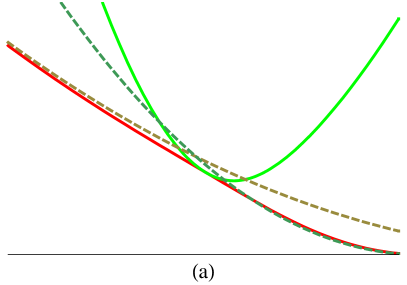
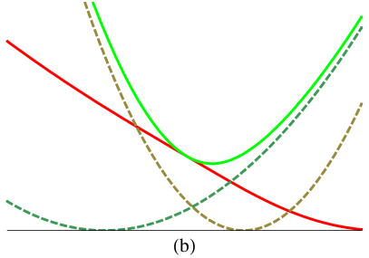
Figure 3: A typical collision between the Dancer cloud and an SU(4) cloud. The horizontal axis represents time, and the vertical axis cloud size. The actual cloud trajectories are shown as solid lines. In (a) the dashed lines indicate the initial and final asymptotic trajectories of the Dancer cloud, while in (b) they indicate the asymptotic trajectories of the SU(4) cloud.

The form of Eq. (22) is strikingly similar to that of Eq. (17), with the Dancer cloud parameter $\tilde{a}$ playing a similar role to $R$, the separation between the massive monopoles in the SU(4) (1,[1],1) solution, and the fixed monopole reduced mass $\mu$ replaced by the variable $\tilde{a}^{-1}$. This seems surprising, since the previous case involved massive monopoles hitting an ellipsoidal cloud at two distinct points, while in the present case two nested spherical clouds are meeting each other at all points. Nevertheless, the similarity in the Lagrangians suggests that the interactions should be similar. In particular, the analysis of the SU(4) dynamics in Ref. Chen:2001ge found that the interaction between the cloud and the massive monopoles was relatively brief, taking place over a distance of order $\mu^{-1}$. This suggests similarly brief interactions in the present case, with the interaction largely restricted to the time when $\delta-\tilde{a}$ is itself of order $\tilde{a}$. We saw some indication of this, with all of the clouds present, in Fig. 2. We illustrate this more clearly in the two-cloud case in Fig. 3, where we show the transition from the initial asymptotic trajectories to the final ones.

Equation (29) suggests that an arbitrary solution depends on four initial constants, $t_{a}$, $t_{\delta}$, $E_{a}$, and $E_{\delta}$. It is clear that time-translation invariance can be used to eliminate one of these. In addition, the Lagrangian of Eq. (22) has some interesting scaling properties. The only effect of the rescalings

$$\tilde{a} \rightarrow \tilde{a}^{\prime}=\lambda\tilde{a}\,,$$ (30)

$$\delta \rightarrow \delta^{\prime}=\lambda\delta\,,$$ (31)

$$t \rightarrow t^{\prime}=\kappa t$$ (32)

is to multiply the Lagrangian by an overall factor of $\lambda/\kappa^{2}$. Hence, given any solution of the equations of motion, these rescalings will generate a two-parameter set of solutions. Thus, to study the full range of possible solutions we really only need to vary a single continuous parameter, which we choose to be $E_{a}/E_{\delta}$. (Note that applying the constraint $\delta>\tilde{a}$ in the asymptotic region implies that $E_{a}/E_{\delta}<4$.) Also, since the rescaling cannot reverse the time ordering, we must consider separately the cases $t_{a}-t_{\delta}>0$ and $t_{a}-t_{\delta}<0$.

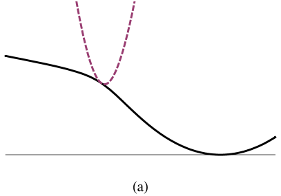
Figure 4: Typical interactions between a Dancer cloud (solid black line) and an SU(4) cloud (dashed purple line). The horizontal axis represents time, and the vertical axis cloud size.

The range of possibilities is illustrated in Fig. 4. If $t_{a}-t_{\delta}>0$, the collapsing SU(4) cloud collides with the Dancer cloud while the latter is also collapsing. Three examples of this are shown in Fig. 4a-c, with the value of $E_{a}/E_{\delta}$ increasing from one to the next. In all three cases the SU(4) cloud loses energy to the Dancer cloud. In the last case, where $E_{a}/E_{\delta}$ is initially close to its maximum allowed value, the SU(4) cloud loses so much energy that the inequality $E_{a}/E_{\delta}<4$ is temporarily violated. Because the cloud radii both increase like $Et^{2}$, there must be a second interaction in which the Dancer cloud overtakes the SU(4) cloud and transfers back enough energy that the inequality is satisfied at large times. The crossover from the behavior shown in Fig. 4b to that in Fig. 4c occurs when $E_{a}/E_{\delta}\approx 2$.

In the borderline case, $t_{a}-t_{\delta}=0$, the two clouds arrive at the origin simultaneously, as shown in Fig. 4d. In this case the asymptotic solution of Eq. (29) is exact for all times, and no energy is exchanged between the clouds.

Finally, we come to the case where $t_{a}-t_{\delta}<0$. Here, the collapsing SU(4) cloud only reaches the Dancer cloud after the latter has already reached its minimum size and begun to expand. If $E_{a}/E_{\delta}<4$ is sufficiently large, as in Fig. 4e, the Dancer cloud loses some energy to the SU(4) cloud, but continues to expand, although at a reduced speed. (This is then a time-reversed version of a solution with $t_{a}-t_{\delta}>0$.) However, if $E_{a}/E_{\delta}<4$ is small enough, as in Fig. 4f, the collision can reverse the expansion of the Dancer cloud and have it shrink to zero radius a second time. The boundary between these two regimes is at $E_{a}/E_{\delta}\approx 2.6$.

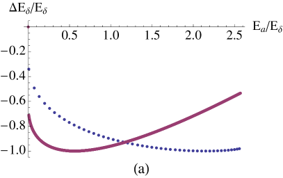
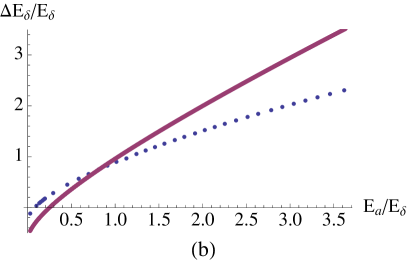
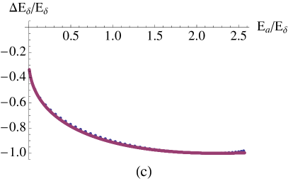
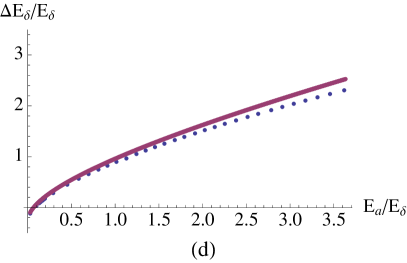
Figure 5: Energy change between the SU(4) and Dancer clouds. In (a) and (c), both clouds are contracting at the time of collision, while in (b) and (d) a contracting SU(4) cloud collides with an expanding Dancer cloud. In all four plots the dotted blue curve shows the transfer observed in the simulations. In (a) and (b) the solid purple curve shows the prediction for an elastic collision, while in (c) and (d) it indicates the prediction for an inelastic collision with $\Delta=-{1\over 5}(3v_{\delta i}^{2}+4v_{\delta i}v_{ai}-4v_{ai}^{2})$.

While these plots are sufficient to provide a qualitative understanding of the interactions, it would be nice to have some more quantitative results as well. Let us first consider the energy transferred during the collision. The fact that the interaction between the clouds takes place over a relatively short time interval suggests a naive model that treats the interaction as an instantaneous elastic collision of two rigid shells, with kinetic energy and radial momentum ($\sum_{a}M_{a}\dot{r}_{a}$) conserved. Because the Dancer cloud has four times the kinetic energy of the SU(4) cloud for the same value of the velocity [see Eq. (26)], we treat it as having four times the mass. It is then a straightforward matter to calculate the fractional energy transfer. The result is compared with the actual data from numerical simulations in Fig. 5. We see that the model captures the important features of the collisions. It accurately predicts that if the two shells collide while traveling in the same direction, the faster one will lose energy. It also agrees with the data in predicting that in a head-on collision the SU(4) cloud will lose almost all of its energy for large values of $E_{a}/E_{\delta}$. Finally, it correctly asserts that for a head-on collision there is a critical value of the initial energy ratio below which the direction of energy transfer is reversed.

This model works better than one might have hoped, but there is no mystery as to why the predicted and observed energy transfer disagree. First, the cloud trajectories are only approximate, and are altered by additional interaction terms that only become significant when the cloud radii are comparable. Second, the interactions are not truly instantaneous, but occur over a finite time interval as the clouds move through one another. Let us modify the statement of conservation of energy of the clouds by including an inelastic term $\Delta$, defined in terms of the initial and final cloud velocities by

$$\frac{1}{2}v_{\delta i}^{2}+\frac{1}{2}v_{ai}^{2}=\frac{1}{2}v_{\delta f}^{2}+\frac{1}{2}v_{af}^{2}+\Delta\,.$$ (33)

Because all of the terms in the conservation of energy equation are quadratic in velocities, we looked for an expression for $\Delta$ that was quadratic in the initial velocities and that provided good agreement with the observed energy transfer. By trial and error, we found that taking $\Delta=-{1\over 5}(3v_{\delta i}^{2}+4v_{\delta i}v_{ai}-4v_{ai}^{2})$ provides excellent agreement with the results obtained from numerical simulations, as can be seen from the plots in Fig. 5. The exact dynamics that give rise to this this formula are still unclear to us.

We argued previously that the interaction between the clouds is largely restricted to the time when $\delta-\tilde{a}$ was itself of order $\tilde{a}$; this gives us a measure of the thickness of the clouds. To describe this more precisely let us define the beginning of the interaction to be the time when 20% of the total energy has been transferred from one cloud to the other, and the end of the interaction to be the time when 80% has been transferred. We also define $\delta_{0}$ and $\tilde{a}_{0}$ to be the values of these variables at the beginning of the interaction and

$$\rho={\delta_{0}-\tilde{a}_{0}\over\tilde{a}_{0}}\,.$$ (34)

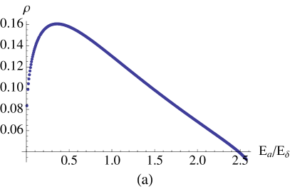
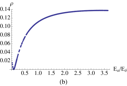
Figure 6: The parameter $\rho$, which is a measure of cloud thickness, as a function of the energy ratio. The result for two collapsing clouds is shown in (a), and for a collapsing SU(4) cloud and expanding Dancer cloud in (b).

Figure 6 shows $\rho$ as a function of energy ratio for two different regimes. The left plot shows $\rho$ for an interaction in which a collapsing SU(4) cloud overtakes a collapsing Dancer cloud. Because the cloud velocities are equal when $E_{a}/E_{\delta}=4$, approaching this value from below corresponds to decreasing the relative velocity of the clouds. This plot therefore shows that $\rho$ decreases as the relative velocity is decreased. We see that the two clouds can approach quite close to one another before exchanging a significant amount of energy if they are moving slowly relative to one another. The right plot is for an interaction in which a collapsing SU(4) cloud collides with an expanding Dancer cloud. In this case the relative velocity increases with $E_{a}/E_{\delta}$. We see that as this increases the clouds begin to transfer their energy sooner, and hence at a greater separation. The maximum value of $\rho$ is about 0.17 in the former case and 0.15 in the latter. The similarity of the values for these two collision scenarios would seem to indicate that the cloud thickness is a relatively small fraction of the cloud radius, approximately $(0.15-0.20)a_{0}$.

The behavior described by these two plots suggests that the clouds act as dissipative media, and that when the SU(4) cloud moves through the Dancer cloud, the energy loss increases with the relative velocity of the clouds. This explains why when both clouds are collapsing and their relative velocity is small, they can come very close together before significant energy is transferred. In the other situation, where the clouds collide head-on, the energy transfer begins very quickly because the relative velocity is large. This is also consistent with the behavior of the inelasticity in the collisions that we found previously.

VI Summary and concluding remarks

In this paper we have used moduli space methods to investigate the properties of the massless magnetic monopoles that arise when a gauge theory is spontaneously broken to a non-Abelian subgroup. We have shown how the natural metric on the Nahm data for a class of SU($2M+2$) solutions with $2M$ massive and $M(2M-1)$ massless monopoles can be obtained from the metric of a simpler class of SU($M+1$) solutions. Using this approach, we have explicitly verified for the SU(4) (1,[1],1) case that the moduli spaces for the Nahm data and for the BPS solutions are isomorphic, thus lending further support to the conjecture that such an isomorphism holds in general. We then applied this method to the problem of obtaining the metric for the SU(6) (2,[2],[2],[2],2) solutions from the (2,[1]) SU(3) metric studied by Dancer. This gave us an effective Lagrangian for a class of axially symmetric solutions. This Lagrangian was then used to study the interactions of the clouds that are the semiclassical manifestation of the massless monopoles.

By examining explicit spacetime solutions, it has been known for some time that the spacetime fields evaluated at the cloud radius are not qualitatively different from those at points slightly further from or closer to the origin. One might therefore expect the interactions between clouds to take place as if the shells of these clouds were diffuse. However, our simulations show instead that the clouds interact more like relatively thin, hard shells. In the collisions between an SU(4) cloud and the Dancer clouds the energy transfer takes place over a short interval before and after the cloud radii coincide, suggesting an effective cloud thickness that is roughly 15-20% of the cloud radius.

Some intriguing open questions remain. It is known that in Type IIB string theory one can interpret D1-branes stretched between D3-branes as the analogs of massive magnetic monopoles. This suggests that massless monopoles should, in some sense, correspond to D1-branes of zero length connecting coincident D3-branes. It would be desirable to clarify these ideas, and to see if they would help explain the properties of the clouds that we have found. One would also like to understand better the role of massless monopoles in the electric-magnetic duality of $N=4$ supersymmetric Yang-Mills theory, where they should be the duals of the “gluons”, the massless gauge particles of the unbroken subgroup. We hope that our results will help shed light on these questions.

*

Appendix A Calculation of $\bm{L_{\rm MS,eff}}$ for the SU(6) example

In this appendix we present the details of the calculation of the moduli space effective Lagrangian, Eq. (24), for the cylindrically symmetric SU(6) solutions of Sec. IV.2.

We begin by calculating the $C_{ab}$. Because none of the $y^{a}$ tangent vectors require a compensating gauge action, Eqs. (31) and (36) for the metric reduce to

$$C_{ab}=4\pi\int_{s_{L}}^{s_{0}}ds\,{\rm Tr\,}{\partial T_{\mu}^{L}\over\partial y^{a}}{\partial T_{\mu}^{L}\over\partial y^{b}}+4\pi\int_{s_{0}}^{s_{R}}ds\,{\rm Tr\,}{\partial T_{\mu}^{R}\over\partial y^{a}}{\partial T_{\mu}^{R}\over\partial y^{b}}+2\pi\,{\rm Tr\,}\left({\partial A\over\partial y^{a}}{\partial A^{\dagger}\over\partial y^{b}}+{\partial A\over\partial y^{b}}{\partial A^{\dagger}\over\partial y^{a}}\right)\,.$$ (1)

The only nonvanishing contributions from the integral over the left interval are

$$I_{ZZ}^{L}\equiv 4\pi\int_{s_{0}}^{s_{L}}ds\,{\rm Tr\,}\left({\partial T_{\mu}^{L}\over\partial Z_{L}}\right)^{2}$$ (2)

and

$$I_{DD}^{L}\equiv 4\pi\int_{s_{0}}^{s_{L}}ds\,{\rm Tr\,}\left({\partial T_{\mu}^{L}\over\partial D_{L}}\right)^{2}\,.$$ (3)

(The mixed integral $I_{ZD}^{L}$ is zero because its integrand vanishes point by point as a result of the trace.) Noting that

$${\partial T^{DL}_{\mu}\over\partial Z_{L}}=\delta_{\mu 3}\,{\rm I}_{2}\,,$$ (4)

we see immediately that

$$I_{ZZ}^{L}=8\pi(s_{0}-s_{L})=2M_{L}\,.$$ (5)

Equation (14) implies that

$$I_{DD}^{L}=2\pi\int_{s_{0}}^{s_{L}}ds\,\left[2\left({\partial g_{1}\over\partial D_{L}}\right)^{2}+\left({\partial g_{3}\over\partial D_{L}}\right)^{2}\right]\,.$$ (6)

Defining $u=s-s_{0}$ and referring to Eq. (21), we see that for the axially symmetric solutions

$${\partial g_{j}\over\partial D_{L}}={1\over D_{L}}\left(g_{j}+ug_{j}^{\prime}\right)\,,$$ (7)

with the prime indicating differentiation with respect to $u$. Hence,

$$I_{DD}^{L} = {2\pi\over D_{L}^{2}}\int_{0}^{M_{L}/(4\pi)}du\left[(2g_{1}^{2}+g_{3}^{2})+2u(2g_{1}g_{1}^{\prime}+g_{3}g_{3}^{\prime})+u^{2}(2g_{1}^{{}^{\prime}2}+g_{3}^{{}^{\prime}2})\right]$$ (8)

$$= {2\pi\over D_{L}^{2}}\int_{0}^{M_{L}/(4\pi)}du\left[g_{3}^{2}+{d\over du}\left(2ug_{1}^{2}+u^{2}g_{1}^{2}g_{3}\right)\right]\,.$$ (9)

[In the second equality we have used Eq. (3) and its cyclic permutations.] This is now easily integrated to give

$$I_{DD}^{L}=\cases{\vphantom{\Biggl{(}}\displaystyle{M_{L}\over 2}(\mu_{L}-\sin\mu_{L}\cos\mu_{L})(\tan\mu_{L}-\mu_{L})\left({\cos\mu_{L}\over\mu_{L}\sin^{3}\mu_{L}}\right)\,,&$\kappa_{L}=0\,,$\cr\cr\vphantom{\Biggl{(}}\displaystyle{M_{L}\over 2}(\mu_{L}-\sinh\mu_{L}\cosh\mu_{L})(\tanh\mu_{L}-\mu_{L})\left({\cosh\mu_{L}\over\mu_{L}\sinh^{3}\mu_{L}}\right)\,,&$\kappa_{L}=1\,,$}$$ (10)

where $\mu_{L}=M_{L}D_{L}/(4\pi)$.

The integrals on the right interval can be evaluated in the same manner, and give the same result, except for the replacement of $M_{L}$, $\mu_{L}$, and $\kappa_{L}$ by $M_{R}$, $\mu_{R}$, and $\kappa_{R}$, respectively.

We need some limiting values of $I_{DD}$. For $\kappa=0$ and $\mu$ close to $\pi$,

$$I_{DD}={\pi M\over 2(\pi-\mu)^{3}}\left[1+O\left({1\over\pi-\mu}\right)\right]\,,$$ (11)

while for $\kappa=1$ and large $\mu$,

$$I_{DD}={M\over 2}\left[1+O\left({1\over\mu}\right)\right]\,.$$ (12)

To calculate the contribution from $A=K^{1/2}$, we recall from Eq. (25) that $K$ can be written in the block diagonal form

$$K=\left(\matrix{\lambda_{1}&0&0\cr 0&\tilde{K}&0\cr 0&0&\lambda_{2}}\right)\,,$$ (13)

where the $2\times 2$ matrix $\tilde{K}$ can be expanded in terms of Pauli matrices as

$$\tilde{K}=(p-C){\rm I}_{2}+2B\rho_{x}+(R-q)\rho_{z}\,.$$ (14)

This can be rewritten as

$$\tilde{K}=U^{-1}PU\,,$$ (15)

where $U=\exp{i\theta\rho_{y}/2}$ with $\tan\theta=2B/(R-q)$ and $P$ is a diagonal matrix with eigenvalues

$$\lambda_{\pm}=(p-C)\pm\sqrt{4B^{2}+(R-q)^{2}}\,.$$ (16)

The square root of $K$ is also block diagonal, with the middle block being $\tilde{K}^{1/2}=U^{-1}P^{1/2}U$, whose derivatives are

$$\partial_{a}\tilde{K}^{1/2}=U^{-1}(\partial_{a}P^{1/2})U+{i\over 2}(\partial_{a}\theta)[U^{-1}P^{1/2}U,\rho_{y}]\,.$$ (17)

To calculate the metric we need

$${\rm Tr\,}\partial_{a}\tilde{K}^{1/2}\partial_{b}\tilde{K}^{1/2} = {\rm Tr\,}\partial_{a}P^{1/2}\partial_{b}P^{1/2}+{i\over 2}(\partial_{a}\theta){\rm Tr\,}\left(\partial_{b}P^{1/2}[P^{1/2},\rho_{y}]\right)$$ (19)

$$\quad+{i\over 2}(\partial_{b}\theta){\rm Tr\,}\left(\partial_{a}P^{1/2}[P^{1/2},\rho_{y}]\right)-{1\over 4}(\partial_{a}\theta)(\partial_{b}\theta){\rm Tr\,}[P^{1/2},\rho_{y}]^{2}\,.$$

Because both $P$ and $\partial_{a}P$ are diagonal, the middle two terms on the right-hand side both vanish. The remaining terms give

$${\rm Tr\,}\partial_{a}\tilde{K}^{1/2}\partial_{b}\tilde{K}^{1/2}=\partial_{a}\sqrt{\lambda_{+}}\,\partial_{b}\sqrt{\lambda_{+}}+\partial_{a}\sqrt{\lambda_{-}}\,\partial_{b}\sqrt{\lambda_{-}}+{1\over 2}(\partial_{a}\theta)(\partial_{b}\theta)\left(\sqrt{\lambda_{+}}-\sqrt{\lambda_{-}}\right)^{2}\,.$$ (21)

Adding to this the contributions from the corner elements of $K$ gives

$${\rm Tr\,}\partial_{a}A\,\partial_{b}A={\rm Tr\,}\partial_{a}K^{1/2}\partial_{b}K^{1/2}=\sum_{\sigma}{\partial_{a}\lambda_{\sigma}\,\partial_{b}\lambda_{\sigma}\over 4\lambda_{\sigma}}+{1\over 2}\partial_{a}\theta\,\partial_{b}\theta\left(\sqrt{\lambda_{+}}-\sqrt{\lambda_{-}}\right)^{2}\,,$$ (22)

where the $\lambda_{\sigma}$ are the four eigenvalues of $K$.

Combining this with our previous results, we obtain.

$$C_{ab}\,dy^{a}dy^{b} = 2M_{L}\,dZ_{L}^{2}+2M_{R}\,dZ_{R}^{2}+I_{DD}^{L}\,dD_{L}^{2}+I_{DD}^{R}\,dD_{R}^{2}$$ (23)

$$+ \pi\left[\sum_{\sigma}{\partial_{a}\lambda_{\sigma}\,\partial_{b}\lambda_{\sigma}\over\lambda_{\sigma}}+2\left(\sqrt{\lambda_{+}}-\sqrt{\lambda_{-}}\right)^{2}\partial_{a}\theta\,\partial_{b}\theta\right]dy^{a}dy^{b}\,.$$ (25)

The next step is to calculate the $B_{2a}$. These only get a contribution from the boundary term, and are given by

$$B_{2a} = -{2\pi i}\,{\rm Tr\,}\left(\left[{\partial A\over\partial y^{a}},A\right]t_{2}\right)$$ (26)

$$= -{2\pi i}\,{\rm Tr\,}\left(\left[{\partial\tilde{K}^{1/2}\over\partial y^{a}},\tilde{K}^{1/2}\right]\rho_{y}\right)\,.$$ (27)

With the aid of Eq. (17), this can be rewritten as

$$B_{2a} = \pi\,\partial_{a}\theta\,{\rm Tr\,}\left\{\left[\left[P^{1/2},\rho_{y}\right],P^{1/2}\right]\rho_{y}\right\}$$ (28)

$$= \pi\,\partial_{a}\theta\,{\rm Tr\,}\left[P^{1/2},\rho_{y}\right]^{2}$$ (30)

$$= {2\pi\,}\partial_{a}\theta\,\left(\sqrt{\lambda_{+}}-\sqrt{\lambda_{-}}\right)^{2}\,.$$ (32)

We also need $E_{22}^{-1}$. Referring to Eqs. (35) and (16), we see that

$$E_{22}^{-1}={1\over 4\pi(\lambda_{+}+\lambda_{-})}\,.$$ (33)

Using these last two results, we can calculate the correction term that converts $L_{\rm MS}$, Eq. (22), to $L_{\rm MS,eff}$, Eq. (24). The terms quadratic in $\partial_{a}\theta$ combine nicely, and we find that

$$\left[C_{ab}-B_{a2}E_{22}^{-1}B_{2b}\right]\,dy^{a}dy^{b} = 2M_{L}\,dZ_{L}^{2}+2M_{R}\,dZ_{R}^{2}+I_{DD}^{L}\,dD_{L}^{2}+I_{DD}^{R}\,dD_{R}^{2}$$ (34)

$$+ \pi\left[\sum_{\sigma}{\partial_{a}\lambda_{\sigma}\,\partial_{b}\lambda_{\sigma}\over\lambda_{\sigma}}+{\left(\lambda_{+}-\lambda_{-}\right)^{2}\over\left(\lambda_{+}+\lambda_{-}\right)}\partial_{a}\theta\,\partial_{b}\theta\right]dy^{a}dy^{b}\,.$$ (36)

References

- (1) K. Lee, E. J. Weinberg and P. Yi, Phys. Rev. D 54, 6351 (1996).
- (2) E. J. Weinberg, Nucl. Phys. B 167, 500 (1980).
- (3) C. Lu, Phys. Rev. D 58, 125010 (1998)
- (4) C. Houghton, P. W. Irwin and A. J. Mountain, JHEP 9904, 029 (1999)
- (5) E. J. Weinberg, Phys. Lett. B 119, 151 (1982).
- (6) E. J. Weinberg and P. Yi, Phys. Rev. D 58, 046001 (1998).
- (7) A. S. Dancer, Nonlinearity 5, 1355 (1992).
- (8) A. S. Dancer, Commun. Math. Phys. 158, 545 (1993).
- (9) A. S. Dancer and R. A. Leese, Proc. Roy. Soc. Lond. A 440 (1993) 421.
- (10) A. S. Dancer and R. A. Leese, Phys. Lett. B 390, 252 (1997).
- (11) C. J. Houghton and E. J. Weinberg, Phys. Rev. D 66, 125002 (2002).
- (12) N. S. Manton, Phys. Lett. B 110, 54 (1982).
- (13) X. Chen and E. J. Weinberg, Phys. Rev. D 64, 065010 (2001).
- (14) N. S. Manton and T. M. Samols, Phys. Lett. B 215, 559 (1988).
- (15) D. Stuart, Commun. Math. Phys. 166, 149 (1994).
- (16) X. Chen, H. Guo and E. J. Weinberg, Phys. Rev. D 64, 125004 (2001).
- (17) M. F. Atiyah and N. J. Hitchin, Phys. Lett. A 107, 21 (1985).
- (18) K. Lee, E. J. Weinberg and P. Yi, Phys. Lett. B 376, 97 (1996).
- (19) J. P. Gauntlett and D. A. Lowe, Nucl. Phys. B 472, 194 (1996).
- (20) W. Nahm, “The construction of all self-dual multimonopoles by the ADHM method”, in Monopoles in Quantum Field Theory, eds. N. S. Craigie et al. (World Scientific, Singapore, 1982).
- (21) W. Nahm, “Multimonopoles in the ADHM construction,” in Gauge Theories and Lepton Hadron Interactions, eds. Z. Horvath et al. (Central Research Institute for Physics, Budapest, 1982).
- (22) W. Nahm, “All self-dual multimonopoles for arbitrary gauge groups,” in Structural Elements in Particle Physics and Statistical Mechanics, eds. J. Honerkamp et al. (Plenum, New York, 1983).
- (23) W. Nahm, “Self-dual monopoles and calorons,” in Group Theoretical Methods in Physics, eds. G. Denardo et (Springer-Verlag, Berlin, 1984).
- (24) H. Nakajima, “Monopoles and Nahm’s equations”, in Einstein Metrics and Yang-Mills Connections, T. Mabuchi and S. Mukai eds. (Marcel Dekker, New York 1993).
- (25) M. Takahasi, Ph.D Thesis, University of Tokyo.
- (26) K. Lee, E. J. Weinberg and P. Yi, Phys. Rev. D 54, 1633 (1996).
- (27) E. J. Weinberg and P. Yi, Phys. Rept. 438, 65 (2007).
- (28) P. Irwin, Phys. Rev. D 56, 5200 (1997).