Quasi-Cyclic LDPC Codes:
Influence of Proto- and Tanner-Graph Structure on Minimum Hamming Distance Upper Bounds

Abstract

Quasi-cyclic (QC) low-density parity-check (LDPC) codes are an important instance of proto-graph-based LDPC codes. In this paper we present upper bounds on the minimum Hamming distance of QC LDPC codes and study how these upper bounds depend on graph structure parameters (like variable degrees, check node degrees, girth) of the Tanner graph and of the underlying proto-graph. Moreover, for several classes of proto-graphs we present explicit QC LDPC code constructions that achieve (or come close to) the respective minimum Hamming distance upper bounds.

Because of the tight algebraic connection between QC codes and convolutional codes, we can state similar results for the free Hamming distance of convolutional codes. In fact, some QC code statements are established by first proving the corresponding convolutional code statements and then using a result by Tanner that says that the minimum Hamming distance of a QC code is upper bounded by the free Hamming distance of the convolutional code that is obtained by “unwrapping” the QC code.

I Introduction

Quasi-cyclic (QC) low-density parity-check (LDPC) codes represent an important class of codes within the family of LDPC codes [1]. The first graph-based code construction that yielded QC codes was presented by Tanner in [2]; although that code construction was presented in the context of repeat-accumulate codes, it was easy to generalize the underlying idea to LDPC codes in order to obtain QC LDPC codes [3, 4, 5, 6]. The simplicity with which QC LDPC codes can be described makes them attractive for implementation and analysis purposes.

A QC LDPC code of length $n=Ir$ can be described by a $Jr\times Ir$ (scalar) parity-check matrix that is formed by a $J\times I$ array of $r\times r$ circulant matrices. Clearly, by choosing these circulant matrices to be low-density, the parity-check matrix will also be low-density.

With the help of the well-known isomorphism between the ring of circulant matrices over some field $\mathbb{F}$ and the ring of $\mathbb{F}$-polynomials modulo $x^{r}-1$ (see, e.g., [7]), a QC LDPC code can equally well be described by a polynomial parity-check matrix of size $J\times I$. In the remainder of the paper we will mainly work with the polynomial parity-check matrix of a QC LDPC code and not with the (scalar) parity-check matrix. Another relevant concept in this paper will be the weight matrix associated with a polynomial parity-check matrix; this weight matrix is a $J\times I$ integer matrix whose entries indicate the number of terms of the corresponding polynomial in the polynomial parity-check matrix.

Early papers on QC LDPC codes focused mainly on polynomial parity-check matrices whose weight matrix contained only ones. Such polynomial parity-check matrices are known as monomial parity-check matrices because all entries are monomials, i.e., polynomials with exactly one term. For this class of QC LDPC codes it was soon established that the minimum Hamming distance is always upper bounded by $(J\!+\!1)!$ [4, 5, 8].

In this paper we study polynomial parity-check matrices with more general weight matrices by allowing the entries of the weight matrix to be $0$, $1$, $2$, or $3$ (and sometimes larger). This is equivalent to allowing the entries of the polynomial parity-check matrix to be the zero polynomial, to be a monomial, to be a binomial, or to be a trinomial (and sometimes a polynomial with more nonzero coefficients). The main theme will be to analyze the minimum Hamming distance of such codes, in particular by studying upper bounds on the minimum Hamming distance and to see how these upper bounds depend on other code parameters like the girth of the Tanner graph. We will obtain upper bounds that are functions of the polynomial parity-check matrix and upper bounds that are functions of the weight matrix. The latter results are in general weaker but they give good insights into the dependency of the minimum Hamming distance on the structure of the weight matrix. For example, for $J=3$ we show that there are weight matrices that are different from the all-one weight matrix (but with the same column and row sum) that yield minimum Hamming distance upper bounds that are larger than the above-mentioned $(J\!+\!1)!$ bound. By constructing some codes that achieve this upper bound we are able to show that the discrepancies in upper bounds are not spurious.

Being able to obtain minimum Hamming distance bounds as a function of the weight matrix is also interesting because the weight matrix is tightly connected to the concept of proto-graphs and LDPC codes derived from them [9, 10]. Proto-graph-based code constructions start with a proto-graph that is described by a $J\times I$ incidence matrix whose entries are non-negative integers and where a “$0$” entry corresponds to no edge, a “$1$” entry corresponds to a single edge, a “$2$” entry corresponds to two parallel edges, etc.. (Such an incidence matrix is also known as a proto-matrix.) Once such a proto-graph is specified, a proto-graph-based LDPC code is then defined to be the code whose Tanner graph [11] is some $r$-fold graph cover [12, 13] of that proto-graph.

It is clear that the construction of QC LDPC codes can then be seen as a special case of the proto-graph-based construction: first, the weight matrix corresponds to the proto-matrix, i.e., the incidence matrix of the proto-graph; secondly, the $r$-fold cover is obtained by restricting the edge permutations to be cyclic.

A main reason for the attractiveness of QC LDPC codes is that they can be encoded efficiently using approaches like in [14] and decoded efficiently using belief-propagation-based decoding algorithms [15] or LP-based decoding algorithms [16, 17, 18, 19]. Although the behavior of these decoders is mostly dominated by pseudo-codewords [20, 21, 22, 23, 24, 25, 26, 27] and the (channel-dependent) pseudo-weight of pseudo-codewords, the minimum Hamming distance still plays an important role because it characterizes undetectable errors and it provides an upper bound on the minimum pseudo-weight of a Tanner graph representing a code.

Although the main focus of this paper is on QC codes, we can state analogous results for convolutional codes. Besides the interest that these statements generate on their own, from a theorem proving point of view these results are helpful because some of our results for QC codes are most easily proven by first proving the corresponding results for convolutional codes. From a technical point of view, this stems from the fact that convolutional codes are defined by parity-check matrices over a field (more precisely, the field $\mathbb{F}_{2}(\!(y)\!)$ specified in Section II-A), whereas QC codes are defined by parity-check matrices over rings (more precisely, the ring $\mathbb{F}_{2}^{\langle r\rangle}[x]$ specified in Section II-A), and that consequently there are more linear algebra tools available to handle convolutional codes than to handle QC codes.

The remainder of this paper is structured as follows. Section II introduces important concepts and the notation that will be used throughout the paper. Thereafter, Section III presents the two main results of this paper. Both results are upper bounds on the minimum Hamming distance of a QC code: whereas in the case of Theorem 7 the upper bound is a function of the polynomial parity-check matrix of the QC code, in the case of Theorem 8 the upper bound is a function of the weight matrix of the QC code only. The following two sections are then devoted to the study of special cases of these results. Namely, Section IV focuses on so-called type-$1$ QC LDPC codes (i.e., QC LDPC codes where the weight matrix entries are at most $1$) and Section V focuses on so-called type-$2$ and type-$3$ QC LDPC codes (i.e., QC LDPC codes where the weight matrix entries are at most $2$ and $3$, respectively). We will show how we can obtain type-$2$ and type-$3$ codes from type-$1$ codes having the same regularity and possibly better minimum Hamming distance properties. Section VI investigates the influence of cycles on minimum Hamming distance bounds. Finally, Section VII discusses a promising construction of type-$1$ QC LDPC codes based on type-$2$ or type-$3$ QC LDPC codes. In fact, we suggest a sequence of constructions starting with a type-$1$ code that exhibits good girth and minimum Hamming distance properties, or that has good performance under message-passing iterative decoding. We construct a type-$2$ or type-$3$ code with the same regularity and higher Hamming distance upper bound, and from this we obtain a new type-$1$ code with possibly larger minimum Hamming distance. Section VIII concludes the paper. The appendix contains the longer proofs and also one section (cf. Appendix I) that lists some results with respect to graph covers.

II Definitions

This section formally introduces the objects that were discussed in Section I, along with some other definitions that will be used throughout the paper.

II-A Sets, Rings, Fields, Vectors, and Matrices

We use the following sets, rings, and fields: for any positive integer $L$, $[L]$ denotes the set $\{0,1,\ldots,L{-}1\}$; $\mathbb{Z}$ is the ring of integers; for any positive integer $r$, $\mathbb{Z}/r\mathbb{Z}$ is the ring of integers modulo $r$; $\mathbb{F}_{2}$ is the Galois field of size $2$; $\mathbb{F}_{2}[x]$ is the ring of polynomials with coefficients in $\mathbb{F}_{2}$ and indeterminate $x$; $\mathbb{F}_{2}[x]/\langle x^{r}{-}1\rangle$ is the ring of polynomials in $\mathbb{F}_{2}[x]$ modulo $x^{r}-1$, where $r$ is a positive integer; and $\mathbb{F}_{2}(\!(y)\!)$ is the field of formal Laurent series over $\mathbb{F}_{2}$, i.e., the set $\bigl{\{}\sum_{\ell=d}^{\infty}a_{\ell}y^{\ell}\bigm{|}d\in\mathbb{Z},\ a_{\ell}\in\mathbb{F}_{2},\ell\geqslant d\bigr{\}}$ with the usual rules for addition and multiplication. We will often use the notational short-hand $\mathbb{F}_{2}^{\langle r\rangle}[x]$ for $\mathbb{F}_{2}[x]/\langle x^{r}{-}1\rangle$.

By $\mathbb{F}_{2}^{n}$ and $\mathbb{F}_{2}^{m\times n}$ we will mean, respectively, a row vector over $\mathbb{F}_{2}$ of length $n$ and a matrix over $\mathbb{F}_{2}$ of size $m\times n$, with a similar meaning given to $\mathbb{F}_{2}^{\langle r\rangle}[x]^{n}$, $\mathbb{F}_{2}^{\langle r\rangle}[x]^{m\times n}$, $\mathbb{F}_{2}(\!(y)\!)^{n}$, and $\mathbb{F}_{2}(\!(y)\!)^{m\times n}$. In the following we will use the convention that indices of vector entries start at $0$ (and not at $1$), with a similar convention for row and column indices of matrix entries.

For any matrix $\mathbf{M}$, we let $\mathbf{M}_{\mathcal{R},\mathcal{S}}$ be the sub-matrix of $\mathbf{M}$ that contains only the rows of $\mathbf{M}$ whose index appears in the set $\mathcal{R}$ and only the columns of $\mathbf{M}$ whose index appears in the set $\mathcal{S}$. If $\mathcal{R}$ equals the set of all row indices of $\mathbf{M}$, we will omit in $\mathbf{M}_{\mathcal{R},\mathcal{S}}$ the set $\mathcal{R}$ and we will simply write $\mathbf{M}_{\mathcal{S}}$. Moreover, we will use the short-hand $\mathbf{M}_{\mathcal{S}\setminus i}$ for $\mathbf{M}_{\mathcal{S}\setminus\{i\}}$.

As usual, the $\min$ operator gives back the minimum value of a list of values. In the following, we will also use a more specialized minimum operator, namely the $\operatorname{min}^{*}$ operator that gives back the minimum value of all nonzero entries in a list of values.

II-B Weights

The weight $\operatorname{wt}\bigl{(}c(x)\bigr{)}\in\mathbb{Z}$ of a polynomial $c(x)\in\mathbb{F}_{2}[x]$ equals the number of nonzero coefficients of $c(x)$. Similarly, the weight $\operatorname{wt}\bigl{(}c(x)\bigr{)}\in\mathbb{Z}$ of a polynomial $c(x)\in\mathbb{F}_{2}^{\langle r\rangle}[x]$ equals the weight $\operatorname{wt}\bigl{(}c^{\prime}(x)\bigr{)}$ of the (unique) minimal-degree polynomial $c^{\prime}(x)\in\mathbb{F}_{2}[x]$ that fulfills $c^{\prime}(x)=c(x)\ (\text{in $\mathbb{F}_{2}^{\langle r\rangle}[x]$})$.

Let $\mathbf{c}(x)=\bigl{(}c_{0}(x),c_{1}(x),\ldots,c_{I-1}(x)\bigr{)}\in\mathbb{F}_{2}^{\langle r\rangle}[x]^{I}$ be a length-$I$ polynomial vector. Then the weight vector $\operatorname{wt}\bigl{(}\mathbf{c}(x)\bigr{)}\in\mathbb{Z}^{I}$ of $\mathbf{c}(x)$ is a length-$I$ vector with the $i$-th entry equal to $\operatorname{wt}\bigl{(}c_{i}(x)\bigr{)}$. Similarly, let $\mathbf{H}(x)=\bigl{[}h_{j,i}(x)\bigr{]}_{j,i}\in\mathbb{F}_{2}^{\langle r\rangle}[x]^{J\times I}$ be a size-$J{\times}I$ polynomial matrix. Then the weight matrix $\operatorname{wt}\bigl{(}\mathbf{H}(x)\bigr{)}\in\mathbb{Z}^{J\times I}$ of $\mathbf{H}(x)$ is a $J{\times}I$-matrix with the entry in row $j$ and column $i$ equal to $\operatorname{wt}\bigl{[}h_{j,i}(x)\bigr{]}$.

The Hamming weight $w_{\mathrm{H}}(\mathbf{c})$ of a vector $\mathbf{c}$ is the number of nonzero entries of $\mathbf{c}$. In the case of a polynomial vector $\mathbf{c}(x)=\bigl{(}c_{0}(x),c_{1}(x),\ldots,c_{I-1}(x)\bigr{)}\in\mathbb{F}_{2}[x]^{I}$, the Hamming weight $w_{\mathrm{H}}\bigl{(}\mathbf{c}(x)\bigr{)}$ is defined to be the sum of the weights of its polynomial entries, i.e., $w_{\mathrm{H}}\bigl{(}\mathbf{c}(x)\bigr{)}=\sum_{i=0}^{I-1}\bigl{(}\operatorname{wt}(\mathbf{c}(x))\bigr{)}_{i}=\sum_{i=0}^{I-1}\operatorname{wt}\bigl{(}c_{i}(x)\bigr{)}$.

Analogous definitions are used for the weight of an element of $\mathbb{F}_{2}(\!(y)\!)$, the weight of vectors over $\mathbb{F}_{2}(\!(y)\!)$, etc..

II-C QC Codes

All codes in this paper will be binary linear codes. As usual, a block code $\mathcal{C}$ of length $n$ can be specified through a (scalar) parity-check matrix $\mathbf{H}\in\mathbb{F}_{2}^{m\times n}$, i.e., $\mathcal{C}=\bigl{\{}\mathbf{c}\in\mathbb{F}_{2}^{n}\ \bigl{|}\ \mathbf{H}\cdot\mathbf{c}^{\mathsf{T}}=\mathbf{0}^{\mathsf{T}}\bigr{.}\bigr{\}}$, where ^T denotes transposition. This code has rate at least $1-\frac{m}{n}$ and its minimum Hamming distance (which equals the minimum Hamming weight since the code is linear) will be denoted by $d_{\mathrm{min}}(\mathcal{C})$.

Let $J$, $I$, and $r$ be positive integers. Let $\mathcal{C}$ be a code of length $Ir$ that possesses a parity-check matrix $\mathbf{H}$ of the form

$$\mathbf{H} =\begin{bmatrix}\mathbf{H}_{0,0}&\mathbf{H}_{0,1}&\cdots&\mathbf{H}_{0,I-1}\\ \mathbf{H}_{1,0}&\mathbf{H}_{1,1}&\cdots&\mathbf{H}_{1,I-1}\\ \vdots&\vdots&\ddots&\vdots\\ \mathbf{H}_{J-1,0}&\mathbf{H}_{J-1,1}&\cdots&\mathbf{H}_{J-1,I-1}\end{bmatrix}\in\mathbb{F}_{2}^{Jr\times Ir},$$

where the sub-matrices $\mathbf{H}_{j,i}\in\mathbb{F}_{2}^{r\times r}$ are circulant. Such a code is called quasi-cyclic (QC) because applying circular shifts to length-$r$ sub-blocks of a codeword gives a codeword again. Because $\mathbf{H}_{j,i}$ is circulant, it can be written as the sum $\mathbf{H}_{j,i}=\sum_{s=0}^{r-1}h_{j,i,s,0}\cdot\mathbf{I}_{s}$, where $h_{j,i,s,0}$ is the entry of $\mathbf{H}_{j,i}$ in row $s$ and column $0$, and where $\mathbf{I}_{s}$ is the $s$ times cyclically left-shifted identity matrix of size $r\times r$.

With a parity-check matrix $\mathbf{H}\in\mathbb{F}_{2}^{Jr\times Ir}$ of a QC code we associate the polynomial parity-check matrix $\mathbf{H}(x)\in\mathbb{F}_{2}^{\langle r\rangle}[x]^{J\times I}$

$$\mathbf{H}(x) =\begin{bmatrix}h_{0,0}(x)&h_{0,1}(x)&\cdots&h_{0,I-1}(x)\\ h_{1,0}(x)&h_{1,1}(x)&\cdots&h_{1,I-1}(x)\\ \vdots&\vdots&\ddots&\vdots\\ h_{J-1,0}(x)&h_{J-1,1}(x)&\cdots&h_{J-1,I-1}(x)\end{bmatrix},$$

where $h_{j,i}(x)\triangleq\sum_{s=0}^{r-1}h_{j,i,s,0}x^{s}$. Moreover, with any vector $\mathbf{c}=(c_{0,0},\ldots,c_{0,r-1},\ldots,c_{I-1,0},\ldots,c_{I-1,r-1})\in\mathbb{F}_{2}^{Ir}$ we associate the polynomial vector

$$\mathbf{c}(x) =\big{(}c_{0}(x),c_{1}(x),\ldots,c_{I-1}(x)\big{)}\in\mathbb{F}_{2}^{\langle r\rangle}[x]^{n},$$

where $c_{i}(x)\triangleq\sum_{s=0}^{r-1}c_{i,s}x^{s}$. It can easily be checked that the condition

$$\mathbf{H}\cdot\mathbf{c}^{\mathsf{T}} =\mathbf{0}^{\mathsf{T}}\quad\text{(in $\mathbb{F}_{2}$)}$$

is equivalent to the condition

$$\mathbf{H}(x)\cdot\mathbf{c}(x)^{\mathsf{T}} =\mathbf{0}^{\mathsf{T}}\quad\text{(in $\mathbb{F}_{2}^{\langle r\rangle}[x]$)},$$

giving us an alternate way to check if a (polynomial) vector is a codeword.

The following classification was first introduced in [8].

Definition 1.

Let $M$ be some positive integer. We say that a polynomial parity-check matrix $\mathbf{H}(x)$ of a QC LDPC code is of type $M$ if all the entries of the associated weight matrix $\operatorname{wt}\bigl{(}\mathbf{H}(x)\bigr{)}$ are at most $M$. Moreover, we say that a QC LDPC code is of type $M$ if it is defined by a polynomial parity-check matrix of type $M$. $\square$

Equivalently, $\mathbf{H}(x)$ is of type $M$ if for each polynomial entry in $\mathbf{H}(x)$ the number of nonzero coefficients is at most $M$. In particular, the polynomial parity-check matrix $\mathbf{H}(x)$ is of type $1$ (in [8] we also called them “type I”) if $\mathbf{H}(x)$ contains only the zero polynomial and monomials. Moreover, the polynomial parity-check matrix $\mathbf{H}(x)$ is of type $2$ (in [8] we also called them “type II”) if $\mathbf{H}(x)$ contains only the zero polynomial, monomials, and binomials. If $\mathbf{H}(x)$ contains only monomials then it will be called a monomial parity-check matrix. (Obviously, a monomial parity-check matrix is a type-$1$ polynomial parity-check matrix.)

II-D Convolutional Codes

A convolutional code $\mathcal{C}_{\mathrm{conv}}$ can be described by a polynomial parity-check matrix $\mathbf{H}_{\mathrm{conv}}(y)\in\mathbb{F}_{2}(\!(y)\!)^{J\times I}$; the codewords of $\mathcal{C}_{\mathrm{conv}}$ are then the polynomial vectors $\mathbf{c}(y)\in\mathbb{F}_{2}(\!(y)\!)^{I}$ that satisfy

$$\mathbf{H}_{\mathrm{conv}}(y)\cdot\mathbf{c}(y)^{\mathsf{T}} =\mathbf{0}^{\mathsf{T}}\quad\text{(in $\mathbb{F}_{2}(\!(y)\!)$)}.$$

The free Hamming distance of $\mathcal{C}_{\mathrm{conv}}$ will be denoted by $d_{\mathrm{free}}(\mathcal{C}_{\mathrm{conv}})$. Moreover, a convolutional code whose (polynomial) parity-check matrix is sparse will be called a convolutional LDPC code and we extend the classification of polynomial parity-check matrices in Definition 1 from QC codes to convolutional codes.

The main interest of the present paper in convolutional codes is the fact that QC codes can be “unwrapped” to yield convolutional codes [28] (see also [29, 30]). In mathematical terms, “unwrapping” means to associate with a QC code $\mathcal{C}$ defined by some polynomial parity-check matrix $\mathbf{H}(x)\in\mathbb{F}_{2}^{\langle r\rangle}[x]^{J\times I}$ the convolutional code $\mathcal{C}_{\mathrm{conv}}$ defined by the parity-check matrix $\mathbf{H}_{\mathrm{conv}}(y)\in\mathbb{F}_{2}(\!(y)\!)^{J\times I}$, where

$$\mathbf{H}_{\mathrm{conv}}(y) \triangleq\mathbf{H}(x)|_{x=y}.$$

In other words, $\mathbf{H}_{\mathrm{conv}}(y)$ is obtained by replacing all appearances of $x$ (and its powers) in $\mathbf{H}(x)$ by $y$ (and its powers). Note that the weight matrices of $\mathbf{H}(x)$ and $\mathbf{H}_{\mathrm{conv}}(y)$ are the same, i.e., $\operatorname{wt}\bigl{(}\mathbf{H}(x)\bigr{)}=\operatorname{wt}\bigl{(}\mathbf{H}_{\mathrm{conv}}(y)\bigr{)}$.

A theorem by Tanner [28] allows one then to relate the minimum Hamming distance of the QC code $\mathcal{C}$ to the free Hamming distance of the above-defined convolutional code $\mathcal{C}_{\mathrm{conv}}$, namely

$$d_{\mathrm{min}}(\mathcal{C}) \leqslant d_{\mathrm{free}}(\mathcal{C}_{\mathrm{conv}}).$$ (1)

(See [31] for the usage of this theorem in the context of QC LDPC and convolutional LDPC codes, along with generalizations of it to different notions of minimum pseudo-weights.)

There is a simple algebraic reason why in the present paper we are interested in the above-mentioned connection between QC codes and convolutional codes. Namely, since the entries of $\mathbf{H}_{\mathrm{conv}}(y)$ are from some field, notions like linear independence and rank are well defined for this matrix. In particular, the zero-ness/nonzero-ness of determinants of square sub-matrices of $\mathbf{H}_{\mathrm{conv}}(y)$ allow us to reach conclusions about the linear dependence/independence of the rows and columns of these sub-matrices. Such conclusions can in general not be reached for the sub-matrices of $\mathbf{H}(x)$, which is a matrix with entries in some commutative ring (in particular, a ring with zero divisors).

II-E Graphs

With a parity-check matrix $\mathbf{H}$ we associate a Tanner graph [11] in the usual way: for every code bit we draw a variable node, for every parity-check we draw a check node, and we connect a variable node and a check node by an edge if and only if the corresponding entry in $\mathbf{H}$ is nonzero. Similarly, the Tanner graph associated with a polynomial parity-check matrix $\mathbf{H}(x)$ is simply the Tanner graph associated with the corresponding (scalar) parity-check matrix $\mathbf{H}$.

As usual, the degree of a vertex is the number of edges incident to it and an LDPC code is called $(d_{1},d_{2})$-regular if all variable nodes have degree $d_{1}$ and all check nodes have degree $d_{2}$. Otherwise we will say that the code is irregular. Moreover, a simple cycle of a graph will be a backtrackless, tailless, closed walk in the graph, and the length of such a cycle is defined to be equal to the number of visited vertices (or, equivalently, the number of visited edges). The girth of a graph is then the length of the shortest simple cycle of the graph.

The above-mentioned concepts are made more concrete with the help of the following example.

Example 2.

Let $\mathcal{C}$ be a length-$12$ QC code that is described by the parity-check matrix

$$\mathbf{H} \triangleq\left[\begin{array}[]{ccc|ccc|ccc|ccc}1&0&1&1&0&0&0&0&0&0&1&0\\ 1&1&0&0&1&0&0&0&0&0&0&1\\ 0&1&1&0&0&1&0&0&0&1&0&0\\ \hline\cr 0&1&0&1&0&0&0&0&1&0&1&0\\ 0&0&1&0&1&0&1&0&0&0&0&1\\ 1&0&0&0&0&1&0&1&0&1&0&0\\ \hline\cr 0&0&0&0&0&1&1&1&0&0&0&1\\ 0&0&0&1&0&0&0&1&1&1&0&0\\ 0&0&0&0&1&0&1&0&1&0&1&0\end{array}\right].$$

Clearly, $J=3$, $I=4$, and $r=3$ for this code and so $\mathbf{H}$ can also be written like

$$\mathbf{H} =\begin{bmatrix}\mathbf{I}_{0}+\mathbf{I}_{1}&\mathbf{I}_{0}&\mathbf{0}&\mathbf{I}_{2}\\ \mathbf{I}_{2}&\mathbf{I}_{0}&\mathbf{I}_{1}&\mathbf{I}_{2}\\ \mathbf{0}&\mathbf{I}_{1}&\mathbf{I}_{0}+\mathbf{I}_{2}&\mathbf{I}_{1}\end{bmatrix},$$

where $\mathbf{I}_{s}$, $s=0,1,\ldots,r{-}1$, are $s$-times cyclically left-shifted $r\times r$ identity matrices. The corresponding polynomial parity-check matrix is

$$\mathbf{H}(x) =\begin{bmatrix}x^{0}+x^{1}&x^{0}&0&x^{2}\\ x^{2}&x^{0}&x^{1}&x^{2}\\ 0&x^{1}&x^{0}+x^{2}&x^{1}\end{bmatrix},$$

and the weight matrix is

$$\operatorname{wt}\big{(}\mathbf{H}(x)\big{)} =\begin{bmatrix}2&1&0&1\\ 1&1&1&1\\ 0&1&2&1\end{bmatrix}.$$

The Tanner graph associated with $\mathbf{H}$ or $\mathbf{H}(x)$ is shown in Figure 1 (left). We observe that all variable nodes have degree $3$ and all check nodes have degree $4$, therefore $\mathcal{C}$ is a $(3,4)$-regular LDPC code. (Equivalently, all columns of $\mathbf{H}$ have weight $3$ and all rows of $\mathbf{H}$ have weight $4$.) $\square$

The proto-graph associated with a polynomial parity-check matrix $\mathbf{H}(x)$ is a graphical representation of the weight matrix $\operatorname{wt}\bigl{(}\mathbf{H}(x)\bigr{)}$ in the following way. It is a graph where for each column of $\mathbf{H}(x)$ we draw a variable node, for each row of $\mathbf{H}(x)$ we draw a check node, and the number of edges between a variable node and a check node equals the corresponding entry in $\operatorname{wt}\bigl{(}\mathbf{H}(x)\bigr{)}$.

Example 3.

Continuing Example 2, the proto-graph of $\mathbf{H}(x)$ is shown in Figure 1 (right). Clearly, the weight matrix $\operatorname{wt}\big{(}\mathbf{H}(x)\big{)}$ is the incidence matrix of this latter graph. We observe that all variable nodes have degree $3$ and all check nodes have degree $4$. (Equivalently, all column sums (in $\mathbb{Z}$) of $\operatorname{wt}\big{(}\mathbf{H}(x)\big{)}$ equal $3$ and all row sums (in $\mathbb{Z}$) of $\operatorname{wt}\big{(}\mathbf{H}(x)\big{)}$ equal $4$.) $\square$

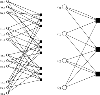
Figure 1: Left: Tanner graph of a length-$12$ QC LDPC code. It is a triple cover of the proto-graph shown on the right. Right: Proto-graph of the Tanner graph shown on the left.

An important concept for this paper is that of the so-called graph covers, see the next definition.

Definition 4 (See, e.g., [12, 13]).

Let $\mathsf{G}$ be a graph with vertex set $\mathcal{V}(\mathsf{G})$ and edge set $\mathcal{E}(\mathsf{G})$, and let $\partial(v)$ denote the set of adjacent vertices of a vertex $v\in\mathcal{V}(\mathsf{G})$. An unramified, finite cover, or, simply, a cover of a (base) graph $\mathsf{G}$ is a graph $\widetilde{\mathsf{G}}$ along with a surjective map $\phi:\widetilde{\mathsf{G}}\to\mathsf{G}$, which is a graph homomorphism, i.e., which takes adjacent vertices of $\widetilde{\mathsf{G}}$ to adjacent vertices of $\mathsf{G}$ such that, for each vertex $v\in\mathcal{V}(\mathsf{G})$ and each $\widetilde{v}\in\phi^{-1}(v)$, the neighborhood $\partial(\widetilde{v})$ of $\widetilde{v}$ is mapped bijectively to $\partial(v)$. For a positive integer $r$, an $r$-cover of $\mathsf{G}$ is an unramified finite cover $\phi:\widetilde{\mathsf{G}}\to\mathsf{G}$ such that, for each vertex $v\in\mathcal{V}(\mathsf{G})$ of $\mathsf{G}$, $\phi^{-1}(v)$ contains exactly $r$ vertices of $\widetilde{\mathsf{G}}$. An $r$-cover of $\mathsf{G}$ is sometimes also called an $r$-sheeted covering of $\mathsf{G}$ or a cover of $\mathsf{G}$ of degree $r$. $\square$

Example 5.

Continuing Examples 2 and 3, we note that the graph in Figure 1 (left) is a $3$-cover of the graph in Figure 1 (right). Therefore, the code $\mathcal{C}$ is a proto-graph-based code. It can easily be checked visually that all edge permutations that were used to define this $3$-cover are cyclic permutations, confirming that the code $\mathcal{C}$ is indeed quasi-cyclic. $\square$

Tanner graphs can also be defined for convolutional codes (see, e.g., [32]); in particular, the paper [32] discusses some connections between the Tanner graph of a QC code and the Tanner graph of a convolutional code that is obtained by “unwrapping” the QC code.

We conclude this subsection by emphasizing that graph covers have been used in two different ways in the context of LDPC codes: on the one hand, they have been used for constructing LDPC codes (like in this paper), on the other hand they have been used to analyze message-passing iterative decoders (like in [23, 24]).

II-F Determinants and Permanents

The determinant of an $m\times m$-matrix $\mathbf{B}=[b_{j,i}]_{j,i}$ over some commutative ring is defined to be

$$\det(\mathbf{B}) =\sum_{\sigma}\operatorname{sgn}(\sigma)\prod_{j\in[m]}b_{j,\sigma(j)},$$

where the summation is over all $m!$ permutations of the set $[m]$, and where $\operatorname{sgn}(\sigma)$ equals $+1$ if $\sigma$ is an even permutation and equals $-1$ if $\sigma$ is an odd permutation.

The permanent of an $m\times m$-matrix $\mathbf{B}=[b_{j,i}]_{j,i}$ over some commutative ring is defined to be

$$\operatorname{perm}(\mathbf{B}) =\sum_{\sigma}\prod_{j\in[m]}b_{j,\sigma(j)},$$

where the summation is over all $m!$ permutations of the set $[m]$.

Clearly, for any matrix $\mathbf{B}$ with elements from a commutative ring of characteristic $2$ it holds that $\det(\mathbf{B})=\operatorname{perm}(\mathbf{B})$.

III Minimum Hamming Distance Upper Bounds

This section contains the two main theoretical results of this paper, namely Theorems 7 and 8. More precisely, given some QC code with polynomial parity-check matrix $\mathbf{H}(x)$ and minimum Hamming distance $d_{\mathrm{min}}(\mathcal{C})$, Theorem 7 presents an upper bound on $d_{\mathrm{min}}(\mathcal{C})$ as a function of the entries of $\mathbf{H}(x)$ and Theorem 8 presents an upper bound on $d_{\mathrm{min}}(\mathcal{C})$ as a function of the entries of $\operatorname{wt}\bigl{(}\mathbf{H}(x)\bigr{)}$. The upper bound of Theorem 8 is in general weaker than the upper bound of Theorem 7, however, it is interesting to see that the weight matrix alone can already give nontrivial bounds on the achievable minimum Hamming distance. These theorems also present analogous results for the free Hamming distance of convolutional codes.

In Sections IV and V, we will discuss the implications of these two theorems on codes with type-$1$, type-$2$, and type-$3$ polynomial parity-check matrices. Moreover, in Section VI we will show how the upper bounds in Theorems 7 and 8 can be strengthened by taking some graph structure information (like cycles) into account.

We start with a simple technique to construct codewords of codes described by polynomial parity-check matrices; this extends a codeword construction technique by MacKay and Davey [4, Theorem 2]. (Note that the paper [4] deals with codes that are described by scalar parity-check matrices composed of commuting permutation sub-matrices, of which parity-check matrices composed of cyclically shifted identity matrices are a special case. However, and as we show in this paper, their techniques can be suitably extended to codes that are described by scalar parity-check matrices composed of any circulant matrices, and therefore to codes that are described by polynomial parity-check matrices.)

Lemma 6.

Let $\mathcal{C}$ be the QC code defined by the polynomial parity-check matrix $\mathbf{H}(x)\in\mathbb{F}_{2}^{\langle r\rangle}[x]^{J\times I}$. Let $\mathcal{S}$ be an arbitrary size-$(J{+}1)$ subset of $[I]$ and let $\mathbf{c}(x)=\big{(}c_{0}(x),c_{1}(x),\ldots,c_{I-1}(x)\big{)}\in\mathbb{F}_{2}^{\langle r\rangle}[x]^{I}$ be a length-$I$ vector defined by

$$c_{i}(x) \triangleq\begin{cases}\operatorname{perm}\big{(}\mathbf{H}_{\mathcal{S}\setminus i}(x)\big{)}&\text{if $i\in\mathcal{S}$}\\ 0&\text{otherwise}\end{cases}.$$

Then $\mathbf{c}(x)$ is a codeword in $\mathcal{C}$.

An analogous construction yields codewords of the convolutional code $\mathcal{C}_{\mathrm{conv}}$ defined by the polynomial parity-check matrix $\mathbf{H}_{\mathrm{conv}}(y)\in\mathbb{F}_{2}(\!(y)\!)^{J\times I}$.

Proof:

Let $\mathcal{S}=\{i_{0},i_{1},\ldots,i_{J}\}$ be the chosen size-$(J{+}1)$ subset. In order to verify that $\mathbf{c}(x)$ is a codeword in $\mathcal{C}$, we need to show that the syndrome $\mathbf{s}^{\mathsf{T}}(x)=\mathbf{H}(x)\cdot\mathbf{c}^{\mathsf{T}}(x)$ (in $\mathbb{F}_{2}^{\langle r\rangle}[x]$) is the all-zero vector. For any $j\in[J]$, we can express the $j$-th component of $\mathbf{s}(x)$ as follows

$$s_{j}(x)=\sum_{i\in[I]}h_{j,i}(x)c_{i}(x) =\sum_{i\in\mathcal{S}}h_{j,i}(x)\cdot\operatorname{perm}\big{(}\mathbf{H}_{\mathcal{S}\setminus i}(x)\big{)}$$

$$=\sum_{i\in\mathcal{S}}h_{j,i}(x)\cdot\det\big{(}\mathbf{H}_{\mathcal{S}\setminus i}(x)\big{)},$$

where in the last step we used the fact that for commutative rings with characteristic $2$ the permanent equals the determinant. Observing that $s_{j}(x)$ is the co-factor expansion of the determinant of the $|\mathcal{S}|\times|\mathcal{S}|$-matrix

$$\left[\begin{array}[]{cccc}h_{j,i_{0}}(x)&h_{j,i_{1}}(x)&\cdots&h_{j,i_{J}}(x)\\ \hline\cr h_{0,i_{0}}(x)&h_{0,i_{1}}(x)&\cdots&h_{0,i_{J}}(x)\\ h_{1,i_{0}}(x)&h_{1,i_{1}}(x)&\cdots&h_{1,i_{J}}(x)\\ \vdots&\vdots&\cdots&\vdots\\ h_{J-1,i_{0}}(x)&h_{J-1,i_{1}}(x)&\cdots&h_{J-1,i_{J}}(x)\\ \end{array}\right],$$

and noting that this latter matrix is singular (because at least two rows are equal), we obtain the result that $\mathbf{s}(x)=\mathbf{0}$ and that $\mathbf{c}(x)$ is indeed a codeword in $\mathcal{C}$, as promised.

Because $\mathbb{F}_{2}(\!(y)\!)$ is a field, and therefore a commutative ring, the same argument holds also for a code like $\mathcal{C}_{\mathrm{conv}}$ that is defined by a parity-check matrix over $\mathbb{F}_{2}(\!(y)\!)$. ∎

With the help of the codeword construction technique in Lemma 6 we can easily obtain the bound in Theorem 7: simply construct the list of all codewords corresponding to all size-$(J{+}1)$ subsets $\mathcal{S}$ of $[I]$, and use the fact that the minimum Hamming distance of $\mathcal{C}$ / the free Hamming distance of $\mathcal{C}_{\mathrm{conv}}$ is upper bounded by the minimum Hamming weight of all nonzero codewords in this list.

Theorem 7.

Let $\mathcal{C}$ be the QC code defined by the polynomial parity-check matrix $\mathbf{H}(x)\in\mathbb{F}_{2}^{\langle r\rangle}[x]^{J\times I}$. Then the minimum Hamming distance of $\mathcal{C}$ is upper bounded as follows

$$d_{\mathrm{min}}(\mathcal{C}) \leqslant\underset{\mathcal{S}\subseteq[I]\atop|\mathcal{S}|=J+1}{\operatorname{min}^{*}}\ \sum_{i\in\mathcal{S}}\operatorname{wt}\Big{(}\operatorname{perm}\big{(}\mathbf{H}_{\mathcal{S}\setminus i}(x)\big{)}\Big{)}.$$ (2)

Let $\mathcal{C}_{\mathrm{conv}}$ be the convolutional code defined by the polynomial parity-check matrix $\mathbf{H}_{\mathrm{conv}}(y)\in\mathbb{F}_{2}(\!(y)\!)^{J\times I}$. Then the free Hamming distance of $\mathcal{C}_{\mathrm{conv}}$ is upper bounded as follows

$$\hskip-5.69046ptd_{\mathrm{free}}(\mathcal{C}_{\mathrm{conv}}) \leqslant\underset{\mathcal{S}\subseteq[I]\atop|\mathcal{S}|=J+1}{\operatorname{min}^{*}}\ \sum_{i\in\mathcal{S}}\operatorname{wt}\Big{(}\operatorname{perm}\big{(}(\mathbf{H}_{\mathrm{conv}})_{\mathcal{S}\setminus i}(y)\big{)}\Big{)}.$$ (3)

(Note that for $\mathbf{H}_{\mathrm{conv}}(y)=\mathbf{H}(x)|_{x=y}$ the right-hand sides of (2) and (3) need not be equal.)

Proof:

We start by proving the QC code part of this theorem. Let $\mathcal{S}$ be a size-$(J\!+\!1)$ subset of $[I]$ and let $\mathbf{c}(x)$ be the corresponding codeword constructed according to Lemma 6. The result in the theorem statement follows by noting that $\mathbf{c}(x)$ has Hamming weight

$$w_{\mathrm{H}}\big{(}\mathbf{c}(x)\big{)} =\sum_{i\in[I]}\operatorname{wt}\big{(}c_{i}(x)\big{)}=\sum_{i\in\mathcal{S}}\operatorname{wt}\big{(}c_{i}(x)\big{)}$$

$$=\sum_{i\in\mathcal{S}}\operatorname{wt}\Big{(}\operatorname{perm}\big{(}\mathbf{H}_{\mathcal{S}\setminus i}(x)\big{)}\Big{)}.$$

The convolutional code part of this theorem then follows from the observation that $\mathbb{F}_{2}(\!(y)\!)$ is a field (and therefore a commutative ring), and so the above derivation also holds for the parity-check matrix $\mathbf{H}_{\mathrm{conv}}(y)$. ∎

Let us emphasize that it is important to have the $\operatorname{min}^{*}$ operator in (2), and not just the $\min$ operator. The reason is that the upper bound is based on constructing codewords of the code $\mathcal{C}$ and evaluating their Hamming weight. For some polynomial parity-check matrices some of these constructed codewords may equal the all-zero codeword and therefore have Hamming weight zero: clearly, such constructed codewords are irrelevant for upper bounding the minimum Hamming distance and therefore must be discarded. This is done with the help of the $\operatorname{min}^{*}$ operator. (Similar statements can be made with respect to (3).)

The next theorem, Theorem 8, gives a minimum/free Hamming distance upper bound which is easier to compute than (2) and (3) and which depends only on the weight matrix associated with $\mathbf{H}(x)$ and $\mathbf{H}_{\mathrm{conv}}(y)$, respectively. In particular, this bound does not depend on $r$, the size of the circulant matrices in the scalar parity-check matrix $\mathbf{H}$ corresponding to $\mathbf{H}(x)$. The bound says that the minimum/free Hamming distance is upper bounded by the minimum nonzero sum of the permanents of all $J\times J$ sub-matrices of a chosen $J\times(J{+}1)$ sub-matrix of the weight matrix, the minimum being taken over all such possible $J\times(J{+}1)$ sub-matrices of the weight matrix.

Theorem 8.

Let $\mathcal{C}$ be a QC code with polynomial parity-check matrix $\mathbf{H}(x)\in\mathbb{F}_{2}^{\langle r\rangle}[x]^{J\times I}$ and let $\mathbf{A}\triangleq\operatorname{wt}\bigl{(}\mathbf{H}(x)\bigr{)}$, or, let $\mathcal{C}_{\mathrm{conv}}$ be a convolutional code with polynomial parity-check matrix $\mathbf{H}_{\mathrm{conv}}(y)\in\mathbb{F}_{2}(\!(y)\!)^{J\times I}$ and let $\mathbf{A}\triangleq\operatorname{wt}\bigl{(}\mathbf{H}_{\mathrm{conv}}(y)\bigr{)}$. Then

$$\left.\begin{array}[]{c}d_{\mathrm{min}}(\mathcal{C})\\[5.69046pt] d_{\mathrm{free}}(\mathcal{C}_{\mathrm{conv}})\end{array}\right\} \leqslant\underset{\mathcal{S}\subseteq[I]\atop|\mathcal{S}|=J+1}{\operatorname{min}^{*}}\ \sum_{i\in\mathcal{S}}\ \operatorname{perm}\left(\mathbf{A}_{\mathcal{S}\setminus i}\right).$$ (6)

In particular, if $\mathbf{H}_{\mathrm{conv}}(y)=\mathbf{H}(x)|_{x=y}$ then

$$d_{\mathrm{min}}(\mathcal{C}) \leqslant d_{\mathrm{free}}(\mathcal{C}_{\mathrm{conv}})\leqslant\underset{\mathcal{S}\subseteq[I]\atop|\mathcal{S}|=J+1}{\operatorname{min}^{*}}\ \sum_{i\in\mathcal{S}}\ \operatorname{perm}\left(\mathbf{A}_{\mathcal{S}\setminus i}\right).$$

Proof:

See Appendix A. ∎

Again, as in Theorem 7, it is important to have the $\operatorname{min}^{*}$ operator in Theorem 8 and not just the $\min$ operator. This time the reasoning is a bit more involved, though, and we refer the reader to the proof of Theorem 8 for details.

Note that the upper bound in (2) depends on $r$ (because the computations are done modulo $x^{r}-1$), whereas the bound in (6) does not depend on $r$.

Usually, the expressions in (2) and (3) yield upper bounds that are not larger than the upper bounds from (6). However, this does not need to happen. For example, there are polynomial parity-check matrices for which (2) and (3) evaluate to $+\infty$, whereas (6) evaluates to some finite number.

Based on Theorems 7 and 8, the following recipe can be formulated for the construction of QC LDPC codes with good minimum Hamming distance. (A similar recipe can be given for the construction of convolutional LDPC codes with good free Hamming distance.)

• Search for a suitable weight matrix with the help of Theorem 8.

• Among all polynomial parity-check matrices with this weight matrix, find a suitable polynomial parity-check matrix with the help of Theorem 7.

• Verify explicitly if the minimum Hamming distance of the code of the found polynomial parity-check matrix really equals (or comes close to) the minimum Hamming distance promised by the upper bound in Theorem 7.

This recipe is especially helpful in the case where one is searching among type-$M$ polynomial parity-check matrices with small $M$, say $M\in\{1,2,3\}$. In such cases it is to be expected that there is not much difference in the upper bounds (2) and (6). For type-$M$ polynomial parity-check matrices with larger $M$, however, we do not expect that the upper bounds (2) and (6) are close. The reason is that when computing $\operatorname{perm}\bigl{(}\mathbf{H}_{\mathcal{S}\setminus i}(x)\bigr{)}$ in (2) there will be many terms that cancel each other. Anyway, when constructing QC LDPC codes, type-$M$ polynomial parity-check matrices with large $M$ are somewhat undesirable because of the relatively small girth of the corresponding Tanner graph. In particular, it is well known that the Tanner graph of a polynomial parity-check matrix whose weight matrix contains at least one entry of weight $3$ (or larger) has girth at most $6$ (see also Theorem 18).

IV Type-I QC/Convolutional Codes

In this section we specialize the results of the previous section to the case of type-$1$ parity-check matrices.

Corollary 9.

Let $\mathcal{C}$ be a type-$1$ QC code with polynomial parity-check matrix $\mathbf{H}(x)\in\mathbb{F}_{2}^{\langle r\rangle}[x]^{J\times I}$ and let $\mathbf{A}\triangleq\operatorname{wt}\bigl{(}\mathbf{H}(x)\bigr{)}$, or, let $\mathcal{C}_{\mathrm{conv}}$ be a type-$1$ convolutional code with polynomial parity-check matrix $\mathbf{H}_{\mathrm{conv}}(y)\in\mathbb{F}_{2}(\!(y)\!)^{J\times I}$ and let $\mathbf{A}\triangleq\operatorname{wt}\bigl{(}\mathbf{H}_{\mathrm{conv}}(y)\bigr{)}$. Then

$$\left.\begin{array}[]{c}d_{\mathrm{min}}(\mathcal{C})\\[5.69046pt] d_{\mathrm{free}}(\mathcal{C}_{\mathrm{conv}})\end{array}\right\} \leqslant(J+1)!.$$ (9)

Proof:

See Appendix B. ∎

The rest of this section will be devoted to QC codes; however, analogous results can also be stated for convolutional codes.

Let us evaluate the minimum Hamming distance upper bounds that we have obtained so far for some type-$1$ QC code polynomial parity-check matrices. (Actually, the following polynomial parity-check matrices happen to be monomial parity-check matrices, i.e., polynomial parity-check matrices where all entries of the corresponding weight matrices equal $1$.)

Example 10.

Let $r\geqslant 9$. Consider the $(2,4)$-regular length-$4r$ QC code $\mathcal{C}$ given by the polynomial parity-check matrix

$${\mathbf{H}}(x)=\begin{bmatrix}x&x^{2}&x^{4}&x^{8}\\ x^{5}&x^{6}&x^{3}&x^{7}\end{bmatrix}$$

and the $(2,4)$-regular length-$4r$ QC code $\mathcal{C}^{\prime}$ given by the polynomial parity-check matrix

$$\mathbf{H}^{\prime}(x)=\begin{bmatrix}x&x^{2}&x^{4}&x^{8}\\ x^{6}&x^{5}&x^{3}&x^{9}\end{bmatrix}.$$

According to (2), the minimum Hamming distance of $\mathcal{C}$ is upper bounded by

$$d_{\mathrm{min}} \leqslant\operatorname{min}^{*}\!\left\{\!\!\!\begin{array}[]{l}\operatorname{wt}(x^{4}{+}x^{9})+\operatorname{wt}(x^{5}{+}x^{10})+\operatorname{wt}(x^{7}{+}x^{7}),\\ \operatorname{wt}(x^{9}{+}x^{14})+\operatorname{wt}(x^{8}{+}x^{13})+\operatorname{wt}(x^{7}{+}x^{7}),\\ \operatorname{wt}(x^{11}{+}x^{11})+\operatorname{wt}(x^{8}{+}x^{13})+\operatorname{wt}(x^{4}{+}x^{9}),\\ \operatorname{wt}(x^{11}{+}x^{11})+\operatorname{wt}(x^{9}{+}x^{14})+\operatorname{wt}(x^{5}{+}x^{10})\end{array}\!\!\!\right\}$$

$$=\operatorname{min}^{*}\{4,4,4,4\}=4,$$

and the minimum Hamming distance of $\mathcal{C}^{\prime}$ is upper bounded by

$$d_{\mathrm{min}} \leqslant\operatorname{min}^{*}\!\left\{\!\!\!\!\begin{array}[]{l}\operatorname{wt}(x^{5}{+}x^{9})\!+\!\operatorname{wt}(x^{4}{+}x^{10})\!+\!\operatorname{wt}(x^{6}{+}x^{8}),\\ \operatorname{wt}(x^{11}{+}x^{13})\!+\!\operatorname{wt}(x^{10}{+}x^{14})\!+\!\operatorname{wt}(x^{6}{+}x^{8}),\\ \operatorname{wt}(x^{13}{+}x^{11})\!+\!\operatorname{wt}(x^{10}{+}x^{14})\!+\!\operatorname{wt}(x^{4}{+}x^{10}),\\ \operatorname{wt}(x^{13}{+}x^{11})\!+\!\operatorname{wt}(x^{11}{+}x^{13})\!+\!\operatorname{wt}(x^{5}{+}x^{9})\end{array}\!\!\!\right\}$$

$$=\operatorname{min}^{*}\{6,6,6,6\}=6.$$

However, in both cases the bound in (6) gives

$$d_{\mathrm{min}} \leqslant\big{\{}(1{+}1)+(1{+}1)+(1{+}1)\big{\}}=6,$$

since both polynomial parity-check matrices have the same weight matrix. Similarly, in both cases the bound in (9) gives

$$d_{\mathrm{min}} \leqslant(2{+}1)!=6,$$

since both polynomial parity-check matrices have $J=2$.

In conclusion, we see that a $2{\times}4$ monomial parity-check matrix can yield a QC code with minimum Hamming distance at most $6$. However, when the entries of the polynomial parity-check matrix are not chosen suitably, as is the case for $\mathbf{H}(x)$, then the minimum Hamming distance upper bound in (2) is strictly smaller than the minimum Hamming distance upper bound in (6).

For completeness, we computed the minimum Hamming distance of the two codes, and obtained $2$ for the first code (e.g., $(0,0,x^{4},1)$ is a codeword), and $4$ for the second code for most values of $r$. $\square$

Let us discuss another example.

Example 11.

Let $r\geqslant 26$ and let the $(3,4)$-regular QC LDPC code $\mathcal{C}$ be given by the polynomial parity-check matrix $\mathbf{H}(x)\in\mathbb{F}_{2}^{\langle r\rangle}[x]^{3\times 4}$

$$\mathbf{H}(x) =\begin{bmatrix}x&x^{2}&x^{4}&x^{8}\\ x^{5}&x^{10}&x^{20}&x^{9}\\ x^{25}&x^{19}&x^{7}&x^{14}\end{bmatrix}.$$

(This code was obtained by shortening the last $r$ positions of the $(3,5)$-regular type-$1$ QC LDPC code of length $5r$ presented in [36].) Evaluating the bounds in (6) and (9) for this polynomial parity-check matrix, we see that the minimum Hamming distance is upper bounded by $24$, and for suitable choices of $r$ this upper bound is indeed achieved. We computed the minimum Hamming distance of the code for different values of $r$ and obtained that $r=31$ is the smallest such choice. The code obtained for $r=31$ has parameters $[124,33,24]$. The minimum Hamming distance and rate for this and some other values of $r$ are listed in the following table.

$r$	$26$	$27$	$28$	$29$	$30$	$31$
$d_{\mathrm{min}}(\mathcal{C})$	$18$	$14$	$16$	$18$	$8$	$24$
rate	0.269	0.287	0.268	0.267	0.283	0.266

$\square$

As we have seen from the above examples, the minimum Hamming distance upper bound (2) can be strictly smaller than the upper bound (6). However, the upper bound (6) is computed more easily, and it provides an upper bound on the Hamming distance of all QC codes having the same weight matrix and therefore also the same proto-graph.

Applying Corollary 9 to QC codes with monomial parity-check matrices shows that for such codes the minimum Hamming distance is upper bounded by $(J{+}1)!$. We note that this result was previously presented by MacKay and Davey [4] and discussed by Fossorier [5]. However, as we show in this paper, their techniques can be suitably extended to QC codes that are described by scalar parity-check matrices composed of any circulant matrices, and therefore to codes that are described by polynomial parity-check matrices.

Example 12.

It is clear that the higher the rate of a code is, the more difficult it is to achieve the upper bound in Corollary 9. However, the QC code defined by the polynomial parity-check matrix

$$\mathbf{H}(x) \triangleq\begin{bmatrix}x^{0}&x^{19}&x^{13}&x^{20}&x^{4}&x^{15}&x^{56}\\ x^{18}&x^{9}&x^{0}&x^{47}&x^{0}&x^{18}&x^{8}\\ x^{14}&x^{0}&x^{10}&x^{13}&x^{0}&x^{0}&x^{7}\end{bmatrix}$$

with $r=111$ shows that there exist also QC codes with design rate $4/7$ that achieve the minimum Hamming distance upper bound in Corollary 9, i.e., $d_{\mathrm{min}}=24$. (This example is taken from [37, Table III].) $\square$

We would like to warn the reader that we do not claim that the “recipe” given at the end of Section III is an optimal strategy for obtaining QC codes that achieve the upper bounds presented in this paper. In particular, instead of fixing the polynomial parity-check matrix and increasing $r$, it might be a good idea to change the polynomial parity-check matrix as well with increasing $r$, thereby allowing the degrees of the polynomials to grow with $r$. Such a strategy might yield codes that achieve the upper bounds for smaller $r$; however, investigating this approach is beyond the scope of this paper.

V Type-II and Type-III
QC/Convolutional Codes

After having discussed minimum/free Hamming distance upper bounds for type-$1$ QC/convolutional codes in the previous section, we now present similar results for type-$2$ and type-$3$ QC/convolutional codes. In particular, we classify all possible weight matrices of $(3,4)$-regular QC/convolutional codes with a $3\times 4$ polynomial parity-check matrix.

We start our investigations with the following motivating example.

Example 13.

In Example 11 we saw that the minimum Hamming distance of type-$1$ $(3,4)$-regular QC codes with a $3\times 4$ polynomial parity-check matrix cannot surpass $24$. In this example we show that type-$2$ $(3,4)$-regular QC codes with a $3\times 4$ polynomial parity-check matrix can have minimum Hamming distance strictly larger than $24$. Namely, consider the code $\mathcal{C}^{\prime}$ with parity-check matrix

$$\hskip-4.26773pt\mathbf{H}^{\prime}(x) \triangleq\begin{bmatrix}x+x^{2}&0&x^{4}&x^{8}\\ x^{5}&x^{9}&x^{10}+x^{20}&0\\ 0&x^{25}+x^{19}&0&x^{7}+x^{14}\end{bmatrix}.$$ (10)

(This polynomial parity-check matrix was obtained from the parity-check matrix $\mathbf{H}(x)$ in Example 11 by pairing some monomials into binomials and replacing with $0$ the positions left, careful to preserve the $(3,4)$-regularity.) The corresponding weight matrix is

$$\mathbf{A}^{\prime} =\begin{bmatrix}2&0&1&1\\ 1&1&2&0\\ 0&2&0&2\end{bmatrix},$$

and, according to (6), yields the following minimum Hamming distance upper bound

$$d_{\mathrm{min}}\left(\mathcal{C}^{\prime}\right) \leqslant\operatorname{min}^{*}\left\{10+6+10+6\right\}=32.$$

For small $r$, the corresponding QC code does not attain this bound, however, for $r=46$ one can verify that the resulting QC code attains the optimal minimum Hamming distance $d_{\mathrm{min}}=32$. This is a $[184,47,32]$ code of rate $0.2554$. $\square$

After this introductory example, let us have a more systematic view of the possible weight matrices of $(3,4)$-regular QC/convolutional codes and the minimum/free Hamming distance upper bounds that they yield.

Corollary 14.

Let $\mathcal{C}$ be a $(3,4)$-regular type-$2$ QC code with polynomial parity-check matrix $\mathbf{H}(x)\in\mathbb{F}_{2}^{\langle r\rangle}[x]^{3\times 4}$ and let $\mathbf{A}\triangleq\operatorname{wt}\bigl{(}\mathbf{H}(x)\bigr{)}\in\mathbb{Z}^{3\times 4}$, or, let $\mathcal{C}_{\mathrm{conv}}$ be a $(3,4)$-regular type-$2$ convolutional code with polynomial parity-check matrix $\mathbf{H}_{\mathrm{conv}}(y)\in\mathbb{F}_{2}(\!(y)\!)^{3\times 4}$ and let $\mathbf{A}\triangleq\operatorname{wt}\bigl{(}\mathbf{H}_{\mathrm{conv}}(y)\bigr{)}\in\mathbb{Z}^{3\times 4}$. Then all possible $(3,4)$-regular size-$(3\!\times\!4)$ type-$2$ weight matrices $\mathbf{A}$ (up to permutations of rows and columns) are given by the following $5$ types of matrices (shown here along with the corresponding minimum/free Hamming distance upper bound implied by (6)):

$$\begin{bmatrix}2&2&0&0\\ 1&1&1&1\\ 0&0&2&2\end{bmatrix}\text{with }\{d_{\mathrm{min}},\,d_{\mathrm{free}}\} \,\leqslant\, 8+8+8+8 =32,$$

$$\begin{bmatrix}2&2&0&0\\ 1&0&2&1\\ 0&1&1&2\end{bmatrix}\text{with }\{d_{\mathrm{min}},\,d_{\mathrm{free}}\} \,\leqslant\, 10+10+6+6 =32,$$

$$\begin{bmatrix}2&0&1&1\\ 1&2&0&1\\ 0&1&2&1\end{bmatrix}\text{with }\{d_{\mathrm{min}},\,d_{\mathrm{free}}\} \,\leqslant\, 7+7+7+9 =30,$$

$$\begin{bmatrix}2&0&1&1\\ 0&2&1&1\\ 1&1&1&1\end{bmatrix}\text{with }\{d_{\mathrm{min}},\,d_{\mathrm{free}}\} \,\leqslant\, 6+6+8+8 =28,$$

$$\begin{bmatrix}1&1&1&1\\ 1&1&1&1\\ 1&1&1&1\end{bmatrix}\text{with }\{d_{\mathrm{min}},\,d_{\mathrm{free}}\} \,\leqslant\, 6+6+6+6 =24.$$

As can be seen from this list, the largest upper bound is $\{d_{\mathrm{min}},\,d_{\mathrm{free}}\}\leqslant 32$ and it can be obtained if the weight matrix $\mathbf{A}$ equals (modulo permutations of rows and columns) the first or the second matrix in the list.

Proof:

Omitted. ∎

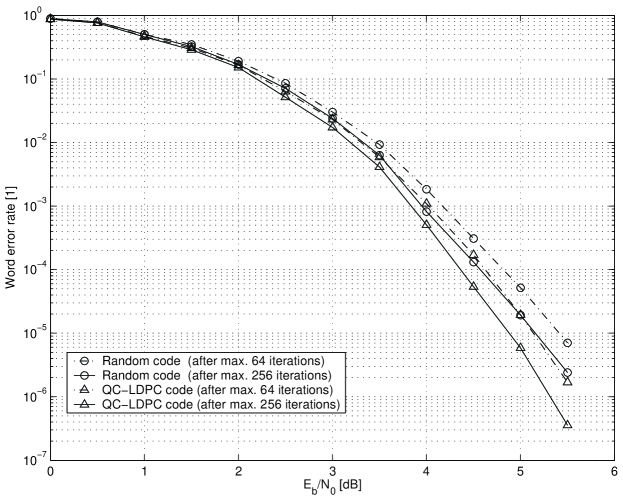
Figure 2: Decoding performance of the $[184,47,32]$ QC LDPC code vs. a randomly generated (four-cycle free) $[184,46]$ LDPC code under sum-product algorithm decoding when transmitting over a binary-input AWGN channel. (For more details, see Example 15.)

Example 15.

We see that the type-$2$ $(3,4)$-regular QC code with a $3\times 4$ polynomial parity-check matrix and with $r=46$ presented in Example 13 not only achieves the minimum Hamming distance upper bound promised by (6) but, according to Corollary 14, it achieves the best possible minimum Hamming distance upper bound for any type-$2$ $(3,4)$-regular QC code with a $3\times 4$ polynomial parity-check matrix. We note that this particular code has parameters $[184,47,32]$, girth $8$, and diameter $8$, i.e., the same girth and diameter as the Tanner graph of the $[124,33,24]$ code in Example 11), which is a shortened version of the $[155,64,20]$ code in [36].

Figure 2 shows the decoding performance (word error rate) of the $[184,47,32]$ QC LDPC code when used for transmission over a binary-input additive white Gaussian noise channel. Decoding is done using the standard sum-product algorithm [15] which is terminated if the syndrome of the codeword estimate is zero or if a maximal number of $64$ (respectively $256$) iterations is reached. It is compared with a randomly generated $(3,4)$-regular $[184,46]$ LDPC code where four-cycles in the Tanner graph have been eliminated. (When comparing these two codes one has to keep in mind that because the randomly generated code has slightly lower rate and because the horizontal axis shows $E_{\mathrm{b}}/N_{0}$, the randomly generated code has a slight “disadvantage” of $0.093\ \mathrm{dB}$.) Note though that the decoding complexity per iteration is the same for both codes.

Let us mention on the side that we tried to estimate the minimum (AWGN channel) pseudo-weight [23, 24] of this code. From searching in the fundamental cone we get an upper bound of $27.6$ on the minimum pseudo-weight. The pseudo-weight spectrum gap [26] is therefore estimated to be $32-27.6=4.4$, which is on the same order as the pseudo-weight spectrum gap for the $(3,5)$-regular $[155,64,20]$ code by Tanner [36], which is estimated to be $20-16.4=3.6$. We also note that for the above-mentioned randomly generated $[184,46]$ code we obtained an upper bound on the minimum pseudo-weight of $21.0$. $\square$

If we want to take into consideration all cases of $(3,4)$-regular QC/convolutional codes with polynomial parity-check matrices of size $3\times 4$, we also have to investigate the class of type-$3$ weight matrices of size $3\times 4$, as is done in the next corollary.

Corollary 16.

Let $\mathcal{C}$ be a $(3,4)$-regular type-$3$ QC code with polynomial parity-check matrix $\mathbf{H}(x)\in\mathbb{F}_{2}^{\langle r\rangle}[x]^{3\times 4}$ and let $\mathbf{A}\triangleq\operatorname{wt}(\mathbf{H}(x))\in\mathbb{Z}^{3\times 4}$, or, let $\mathcal{C}_{\mathrm{conv}}$ be a $(3,4)$-regular type-$3$ convolutional code with polynomial parity-check matrix $\mathbf{H}_{\mathrm{conv}}(y)\in\mathbb{F}_{2}(\!(y)\!)^{3\times 4}$ and let $\mathbf{A}\triangleq\operatorname{wt}(\mathbf{H}(x))\in\mathbb{Z}^{3\times 4}$. Then all possible $(3,4)$-regular size-$(3\!\times\!4)$ type-$3$ weight matrices $\mathbf{A}$ (up to permutations of rows and columns) are given by the $5$ types of matrices already listed in Corollary 14, together with the following $3$ types of matrices (shown here along with the corresponding minimum/free Hamming distance upper bound implied by (6)):

$$\begin{bmatrix}3&0&0&1\\ 0&2&1&1\\ 0&1&2&1\end{bmatrix}\text{with }\{d_{\mathrm{min}},\,d_{\mathrm{free}}\} \,\leqslant\, 5+9+9+15 =38,$$

$$\begin{bmatrix}3&1&0&0\\ 0&2&1&1\\ 0&0&2&2\end{bmatrix}\text{with }\{d_{\mathrm{min}},\,d_{\mathrm{free}}\} \,\leqslant\, 4+12+12+12 =40,$$

$$\begin{bmatrix}3&0&0&1\\ 0&3&0&1\\ 0&0&3&1\end{bmatrix}\text{with }\{d_{\mathrm{min}},\,d_{\mathrm{free}}\} \,\leqslant\, 9+9+9+27 =54.$$

As it can easily be seen, the largest upper bound is $\{d_{\mathrm{min}},\,d_{\mathrm{free}}\}\leqslant 54$ and it can be obtained if the weight matrix $\mathbf{A}$ equals (modulo permutations of rows and columns) the last matrix in the above list.

Proof:

Omitted. ∎

Example 17.

We can modify the matrix $\mathbf{H}$ in Example 11 to obtain one of the configurations in Corollary 16. For example, the following matrix ${\mathbf{H}}^{\prime}(x)\in\mathbb{F}_{2}^{\langle r\rangle}[x]^{3\times 4}$ corresponds to the last configuration listed in Corollary 16:

$$\mathbf{H}^{\prime}(x) \triangleq\begin{bmatrix}x^{2}{+}x^{4}{+}x^{8}&0&0&x\\ 0&x^{9}{+}x^{10}{+}x^{20}&0&x^{5}\\ 0&0&x^{19}{+}x^{7}{+}x^{14}&x^{25}\end{bmatrix}.$$

For $r=31$ we obtain a $[124,31,28]$ code, whose rate is $0.25$. (In comparison, the monomial $[124,33,24]$ QC LDPC code in Example 11 has rate $0.266$ and the binomial $[184,47,32]$ QC LDPC code in Example 13 has rate $0.2554$.) For $r=46$, we obtain a code with parameters $[184,46,34]$. For larger $r$ the minimum Hamming distance could increase up to $54$. $\square$

Note that the Tanner graph of a polynomial parity-check matrix which has at least one trinomial entry cannot have girth larger than $6$ (see, e.g., [5]). We state this observation as part of a more general analysis of the effect of the weight matrix on the girth.

Theorem 18.

Let $\mathcal{C}$ be a QC code described by a polynomial parity-check matrix $\mathbf{H}(x)\in\mathbb{F}_{2}^{\langle r\rangle}[x]^{J\times I}$, let $\operatorname{girth}$ be the girth of the Tanner graph corresponding to $\mathbf{H}(x)$ and let $\mathbf{A}$ be the weight matrix corresponding to $\mathbf{H}(x)$. Or, let $\mathcal{C}_{\mathrm{conv}}$ be a convolutional code described by a polynomial parity-check matrix $\mathbf{H}_{\mathrm{conv}}(y)\in\mathbb{F}_{2}(\!(y)\!)^{J\times I}$, let $\operatorname{girth}$ be the girth of the Tanner graph corresponding to $\mathbf{H}_{\mathrm{conv}}(y)$ and let $\mathbf{A}$ be the weight matrix corresponding to $\mathbf{H}_{\mathrm{conv}}(y)$.

1. If $\mathbf{A}$ has sub-matrix $\begin{bmatrix}1&1&1\\ 1&1&1\end{bmatrix}$ then $\operatorname{girth}\leqslant 12$.
   

2. If $\mathbf{A}$ has sub-matrix $\begin{bmatrix}1&1\\ 1&2\end{bmatrix}$ then $\operatorname{girth}\leqslant 10$.
   

3. If $\mathbf{A}$ has sub-matrix $\begin{bmatrix}2&2\end{bmatrix}$ then $\operatorname{girth}\leqslant 8$.
   

4. If $\mathbf{A}$ has sub-matrix $\begin{bmatrix}3\end{bmatrix}$ then $\operatorname{girth}\leqslant 6$.

(By “$\mathbf{A}$ having sub-matrix $\mathbf{B}$” we mean that $\mathbf{A}$ contains a sub-matrix that is equivalent to $\mathbf{B}$, modulo row permutations, column permutations, and transposition.)

Proof:

See Appendix C. ∎

The Corollaries 14 and 16 focused on the case of $(3,4)$-regular QC/convolutional codes with a $3\times 4$ polynomial parity-check matrix. It is clear that similar results can be formulated for any $(J^{\prime},I^{\prime})$-regular QC/convolutional code with a $J\times I$ polynomial parity-check matrix. However, we will not elaborate this any further, except for mentioning the following corollary about $(3,5)$-regular QC/convolutional codes with a $3\times 5$ polynomial parity-check matrix.

Corollary 19.

An optimal $(3,5)$-regular type-$2$ weight matrix of size $3\times 5$ must (up to row and column permutations) look like

$$\mathbf{A} \triangleq\begin{bmatrix}2&2&1&0&0\\ 0&0&2&2&1\\ 1&1&0&1&2\end{bmatrix}.$$

This weight matrix yields the upper bound

$$\{d_{\mathrm{min}},\,d_{\mathrm{free}}\} \leqslant\min\{30,30,30,32,28\}=28.$$

Proof:

Omitted. ∎

It would be desirable to obtain simply looking bounds for type-$2$ and type-$3$ codes with $(J,I)$-regular parity-check matrices of size $J\times I$. Although it is straightforward to obtain such simple bounds by suitably generalizing the derivation of Corollary 9, the resulting bounds are usually not very useful. We leave it as an open problem to find such relevant bounds in the style of Corollary 9 for type-$2$ and type-$3$ codes.

VI The Effect of Small Cycles
on the Minimum Hamming Distance
and the Free Hamming Distance

If we know that the Tanner graph corresponding to some polynomial parity-check matrix contains some short cycles then we can strengthen the upper bounds of Theorem 7 and 8. In particular, Theorems 22, 25, and 26 will study the influence of $4$-cycles, $6$-cycles, and $2R$-cycles, respectively, upon the minimum/free Hamming distance upper bounds. These theorems will be based on results presented in Lemmas 20 and 24 that characterize cycles in Tanner graphs in terms of some entries of the corresponding polynomial parity-check matrix, especially in terms of permanents of sub-matrices. In order to state such conditions, we will use results from [36, 5]. (For other cycle-characterizing techniques and results, see also [38] and [39].)

As we will see, the smaller the girth of the Tanner graph, the smaller the minimum/free Hamming distance upper bound will be. This observation points in the same direction as other results do that relate the decoding performance of LDPC codes (especially under message-passing iterative decoding) to the girth of their Tanner graph: firstly, there is a lot of empirical evidence that smaller girth usually hurts the iterative decoding performance; secondly, there are results concerning the structure of the fundamental polytope that show that the fundamental polytope of Tanner graphs with smaller girth is “weaker,” see, e.g., [24, Section 8.3], [40].

VI-A Type-I QC/Convolutional Codes with $4$-Cycles

Lemma 20.

The Tanner graph of a type-$1$ QC code $\mathcal{C}$ with polynomial parity-check matrix $\mathbf{H}(x)\in\mathbb{F}_{2}^{\langle r\rangle}[x]^{J\times I}$ has a $4$-cycle if and only if $\mathbf{H}(x)$ has a $2\times 2$ sub-matrix $\mathbf{B}(x)$ for which

$$\operatorname{wt}\Big{(}\operatorname{perm}\big{(}\mathbf{B}(x)\big{)}\Big{)}<\operatorname{perm}\Big{(}\operatorname{wt}\big{(}\mathbf{B}(x)\big{)}\Big{)}$$

holds.

An analogous statement can be made for the Tanner graph of a type-$1$ convolutional code $\mathcal{C}_{\mathrm{conv}}$ defined by the polynomial parity-check matrix $\mathbf{H}_{\mathrm{conv}}(y)\in\mathbb{F}_{2}(\!(y)\!)^{J\times I}$.

Proof:

See Appendix D. ∎

Corollary 21.

The Tanner graph of a type-$1$ QC code $\mathcal{C}$ with polynomial parity-check matrix $\mathbf{H}(x)\in\mathbb{F}_{2}^{\langle r\rangle}[x]^{J\times I}$ has a $4$-cycle if and only if $\mathbf{H}(x)$ has a $2\times 2$ sub-matrix $\mathbf{B}(x)$ which is monomial and for which $\operatorname{perm}\bigl{(}\mathbf{B}(x)\bigr{)}=0$ (in $\mathbb{F}_{2}^{\langle r\rangle}[x]$) holds.

An analogous statement can be made for the Tanner graph of a type-$1$ convolutional code $\mathcal{C}_{\mathrm{conv}}$ with polynomial parity-check matrix $\mathbf{H}_{\mathrm{conv}}(y)\in\mathbb{F}_{2}(\!(y)\!)^{J\times I}$.

Proof:

This follows from Lemma 20 and its proof. ∎

With this, we are ready to investigate minimum/free Hamming distance upper bounds for Tanner graphs with $4$-cycles.

Theorem 22.

Let $\mathcal{C}$ be a type-$1$ QC code with polynomial parity-check matrix $\mathbf{H}(x)\in\mathbb{F}_{2}^{\langle r\rangle}[x]^{J\times I}$, or, let $\mathcal{C}_{\mathrm{conv}}$ be a type-$1$ convolutional code with polynomial parity-check matrix $\mathbf{H}_{\mathrm{conv}}(y)\in\mathbb{F}_{2}(\!(y)\!)^{J\times I}$. If the associated Tanner graph has a $4$-cycle then

$$\left.\begin{array}[]{c}d_{\mathrm{min}}(\mathcal{C})\\[5.69046pt] d_{\mathrm{free}}(\mathcal{C}_{\mathrm{conv}})\end{array}\right\} \leqslant(J{+}1)!\,-\,2(J{-}1)!.$$ (13)

Proof:

See Appendix E. ∎

Example 23.

Let us consider again the $(2,4)$-regular length-$4r$ QC code $\mathcal{C}$ from Example 10 which is given by the polynomial parity-check matrix

$$\mathbf{H}(x) =\begin{bmatrix}x&x^{2}&x^{4}&x^{8}\\ x^{5}&x^{6}&x^{3}&x^{7}\end{bmatrix}.$$

It has at least two $4$-cycles since

$$\operatorname{perm}\left(\begin{bmatrix}x&x^{2}\\ x^{5}&x^{6}\end{bmatrix}\right) =0\quad\text{and}\quad\operatorname{perm}\left(\begin{bmatrix}x^{4}&x^{8}\\ x^{3}&x^{7}\end{bmatrix}\right)=0\;$$

(in $\mathbb{F}_{2}^{\langle r\rangle}[x]$). Therefore the bound (13) gives

$$d_{\mathrm{min}}(\mathcal{C}) \leqslant(J{+}1)!\,-\,2(J{-}1)!=3!-2\cdot 1!=4.$$ (14)

We note that for this $\mathbf{H}(x)$ this upper bound equals the upper bound (2) (cf. Example 10). $\square$

VI-B Type-I QC/Convolutional Codes with $6$-Cycles

Lemma 24.

The Tanner graph of a type-$1$ QC LDPC code $\mathcal{C}$ with polynomial parity-check matrix $\mathbf{H}(x)\in\mathbb{F}_{2}^{\langle r\rangle}[x]^{J\times I}$ has a $6$-cycle (or possibly a $4$-cycle) if and only if $\mathbf{H}(x)$ has a $3\times 3$ sub-matrix $\mathbf{B}(x)$ for which

$$\operatorname{wt}\Big{(}\operatorname{perm}\big{(}\mathbf{B}(x)\big{)}\Big{)} <\operatorname{perm}\Big{(}\operatorname{wt}\big{(}\mathbf{B}(x)\big{)}\Big{)}$$

holds, i.e., if and only if $\mathbf{H}(x)$ has a $3\times 3$ sub-matrix $\mathbf{B}(x)$ for which some terms of its permanent expansion add to zero.

An analogous statement can be made for the Tanner graph of a type-$1$ convolutional code $\mathcal{C}_{\mathrm{conv}}$ defined by the polynomial parity-check matrix $\mathbf{H}_{\mathrm{conv}}(y)\in\mathbb{F}_{2}(\!(y)\!)^{J\times I}$.

Proof:

See Appendix F. ∎

With this, we are ready to investigate the minimum/free Hamming distance upper bounds for Tanner graphs with $6$-cycles.

Theorem 25.

Let $\mathcal{C}$ be a type-$1$ QC code with polynomial parity-check matrix $\mathbf{H}(x)\in\mathbb{F}_{2}^{\langle r\rangle}[x]^{J\times I}$, or, let $\mathcal{C}_{\mathrm{conv}}$ be a type-$1$ convolutional code with polynomial parity-check matrix $\mathbf{H}_{\mathrm{conv}}(y)\in\mathbb{F}_{2}(\!(y)\!)^{J\times I}$. If the associated Tanner graph has a $6$-cycle then

$$\left.\begin{array}[]{c}d_{\mathrm{min}}(\mathcal{C})\\[5.69046pt] d_{\mathrm{free}}(\mathcal{C}_{\mathrm{conv}})\end{array}\right\}\leqslant(J{+}1)!\,-\,2(J{-}2)!.$$

Proof:

See Appendix G. ∎

VI-C Type-I QC/Convolutional Codes with $2R$-Cycles

The previous two subsections have shown that the minimum Hamming distance of a type-$1$ QC/convolutional code whose Tanner graph has girth $4$ or $6$ can never attain the maximal value $(J{+}1)!$ of Corollary 9. These results are special cases of a more general result that we will discuss next. Note however that, compared to the girth-$4$ and the girth-$6$ case, this more general statement is uni-directional.

Theorem 26.

Let $\mathcal{C}$ be a type-$1$ QC code with polynomial parity-check matrix $\mathbf{H}(x)=[h_{j,i}(x)]_{j,i}\in\mathbb{F}_{2}^{\langle r\rangle}[x]^{J\times I}$. Let $R$, $2\leqslant R\leqslant\min(J,I)$, be some integer, and suppose there is a set $\mathcal{R}\subseteq[J]$ of size $R$, a set $\mathcal{S}\subseteq[I]$ of size $R$, and two distinct bijective mappings $\sigma$ and $\tau$ from $\mathcal{R}$ to $\mathcal{S}$ such that $\sigma(j)\neq\tau(j)$ for all $j\in\mathcal{R}$ and such that

$$\prod_{j\in\mathcal{R}}h_{j,\sigma(j)}(x) =\prod_{j\in\mathcal{R}}h_{j,\tau(j)}(x).$$ (15)

Then

$$d_{\mathrm{min}} \leqslant(J{+}1)!\,-\,2(J{-}R{+}1)!.$$

If, in addition, the (bijective) mapping $\sigma^{-1}\circ\tau$ from $\mathcal{R}$ to $\mathcal{R}$ is a cyclic permutation of order $R$ and if the products on the left-hand and right-hand side of the equation in (15) are nonzero, then the associated Tanner graph will have a cycle of length $2R$.

An analogous statement can be made for the Tanner graph of a type-$1$ convolutional code $\mathcal{C}_{\mathrm{conv}}$ defined by the polynomial parity-check matrix $\mathbf{H}_{\mathrm{conv}}(y)\in\mathbb{F}_{2}(\!(y)\!)^{J\times I}$.

Proof:

See Appendix H. ∎

For $4$- and $6$-cycles, the converse of the second part of the above corollary is true, i.e., $4$- and $6$-cycles are visible in, respectively, $2\times 2$ and $3\times 3$ sub-matrices (cf. Theorems 22 and 25). However, for longer cycles the converse of the second part of the above corollary is not always true: $8$-cycles can happen in $4\times 4$ sub-matrices, but also in $2\times 4$ sub-matrices or in $3\times 4$ sub-matrices. A similar statement holds for longer cycles.

VI-D Type-II QC/Convolutional Codes

With appropriate techniques/computations, similar statements as in the preceding subsection can also be made about type-$2$ QC/convolutional codes. We will not say much about this topic except for stating a lemma that helps in detecting if a polynomial parity-check matrix is $4$-cycle free.

Lemma 27.

A type-$2$ QC code $\mathcal{C}$ is $4$-cycle free if and only if its polynomial parity-check matrix $\mathbf{H}(x)$ has the following properties.

1. If $r$ is even, then for any $1\times 1$ sub-matrix like

   $$\begin{bmatrix}x^{a}+x^{b}\end{bmatrix}$$

   it holds that the permanent of

   $$\begin{bmatrix}x^{a}&x^{b}\\ x^{b}&x^{a}\end{bmatrix}$$

   is nonzero (in $\mathbb{F}_{2}^{\langle r\rangle}[x]$). (This condition is equivalent to the condition $x^{2a}+x^{2b}\neq 0\ \text{(in $\mathbb{F}_{2}[x]$)}$, or to the condition $\gcd(x^{a}+x^{b},1+x^{r})\neq 1+x^{r/2}\ \text{(in $\mathbb{F}_{2}[x]$)}$.)

2. For any $1\times 2$ sub-matrix like

   $$\begin{bmatrix}x^{a}+x^{b}&x^{c}+x^{d}\end{bmatrix}\;,$$

   or any $2\times 1$ sub-matrix like

   $$\begin{bmatrix}x^{a}+x^{b}\\ x^{c}+x^{d}\end{bmatrix}\;,$$

   the product $(x^{a}+x^{b})\cdot(x^{c}+x^{d})$ (in $\mathbb{F}_{2}^{\langle r\rangle}[x]$) has weight $4$, i.e., the maximally possible weight, or, equivalently, if all the $2\times 2$ sub-matrices of the matrix

   $$\begin{bmatrix}x^{a}&x^{b}&x^{c}&x^{d}\\ x^{b}&x^{a}&x^{d}&x^{c}\end{bmatrix}\;,$$

   have nonzero permanent (in $\mathbb{F}_{2}^{\langle r\rangle}[x]$).

3. For any $2\times 2$ sub-matrix like

   $$\begin{bmatrix}x^{a}&x^{b}+x^{c}\\ x^{d}+x^{e}&x^{f}\end{bmatrix}$$

   (or row and column permutations thereof), the permanents (in $\mathbb{F}_{2}^{\langle r\rangle}[x]$) of the following two $2\times 2$ sub-matrices

   $$\begin{bmatrix}x^{a}&x^{b}\\ x^{d}+x^{e}&x^{f}\end{bmatrix}\text{ \ and \ }\begin{bmatrix}x^{a}&x^{c}\\ x^{d}+x^{e}&x^{f}\end{bmatrix}$$

   have weight $3$, the maximally possible weight, or, equivalently, if all $2\times 2$ sub-matrices of the matrix

   $$\begin{bmatrix}x^{a}&0&x^{b}&x^{c}\\ 0&x^{a}&x^{c}&x^{b}\\ x^{d}&x^{e}&x^{f}&0\\ x^{e}&x^{d}&0&x^{f}\end{bmatrix}$$

   have nonzero permanent (in $\mathbb{F}_{2}^{\langle r\rangle}[x]$).

4. For any $2\times 2$ sub-matrix with weight matrix

   $$\begin{bmatrix}2&2\\ 1&1\end{bmatrix},\begin{bmatrix}2&1\\ 1&1\end{bmatrix},\text{ \ and \ }\begin{bmatrix}1&1\\ 1&1\end{bmatrix}$$

   (or row and column permutations thereof), the permanent (in $\mathbb{F}_{2}^{\langle r\rangle}[x]$) of this $2\times 2$ sub-matrix has weight $4$, $3$, and $2$, respectively, i.e., the maximally possible weight.

An analogous statement holds for the Tanner graph of a type-$2$ convolutional code $\mathcal{C}_{\mathrm{conv}}$ defined by the polynomial parity-check matrix $\mathbf{H}_{\mathrm{conv}}(y)\in\mathbb{F}_{2}(\!(y)\!)^{J\times I}$.

Proof:

It is well known that a $4$-cycle appears in a Tanner graph if and only if the corresponding (scalar) parity-check matrix contains the $2\times 2$ (scalar) sub-matrix

$$\begin{bmatrix}1&1\\ 1&1\end{bmatrix}\;.$$

The lemma is then proved by studying all possible cases in which a polynomial parity-check matrix can lead to a (scalar) parity-check that contains this $2\times 2$ (scalar) sub-matrix. The details are omitted. ∎

Note that in the above lemma some of the conditions were expressed in terms of a double cover of the relevant sub-matrices. In particular, the modified matrices are obtained by applying the following changes to the entries of the relevant sub-matrices

$$x^{a}+x^{b} \mapsto\begin{bmatrix}x^{a}&x^{b}\\ x^{b}&x^{a}\end{bmatrix},$$

$$x^{f} \mapsto\begin{bmatrix}x^{f}&0\\ 0&x^{f}\end{bmatrix},$$

$$0 \mapsto\begin{bmatrix}\ 0\ &\ 0\ \\ \ 0\ &\ 0\ \end{bmatrix}.$$

(Note that similar double covers are also considered in Appendix I.)

Example 28.

Consider, for $r\geqslant 26$, the type-$2$ polynomial parity-check matrix $\mathbf{H}^{\prime}(x)$ in (10). There, $4$-cycles could only be caused by the two sub-matrices

$$\begin{bmatrix}x^{1}+x^{2}&x^{4}\\ x^{5}&x^{10}+x^{20}\end{bmatrix}\quad\text{and}\quad\begin{bmatrix}x^{25}+x^{19}&x^{7}+x^{14}\end{bmatrix}\;.$$

Therefore, the conditions for the non-existence of a $4$-cycle are

$$0 \notin\{5-1,5-2\}+\{4-10,4-20\}\quad\text{(in $\mathbb{Z}/r\mathbb{Z}$)}\;,$$

$$0 \notin\{25-19,19-25\}+\{7-14,14-7\}\quad\text{(in $\mathbb{Z}/r\mathbb{Z}$)}\;.$$

(Here the sum of two sets denotes the set of all possible sums involving one summand from the first set and one summand from the second set.) It is clear that, with suitable effort, similar analyses could be made for the non-existence of longer cycles. $\square$

VII Type-I QC Codes based on
Double Covers of Type-II QC Codes

So far, we have mostly considered $(J,I)$-regular QC codes that are described by a $J\times I$ polynomial parity-check matrix. However, one can construct many interesting $(J^{\prime},I^{\prime})$-regular QC LDPC codes with a $J\times I$ polynomial parity-check matrix where $J^{\prime}\neq J$ and/or $I^{\prime}\neq I$. Given the enormity of the search space, a worthwhile approach is to start with some small code that has good properties and to derive longer codes from it. In this section we present such an approach, along with an analysis of it. Of course, there are many other possibilities; we leave them open to future studies. (Note that this section deals only with QC codes, however, similar investigations can also be pursued for convolutional codes.)

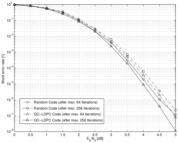
Figure 3: Decoding performance of the $[368,93,32]$ QC LDPC code $\mathcal{\tilde{C}}$ and the $[368,93,56]$ QC LDPC code $\mathcal{\hat{C}}$ from Example 29 vs. a randomly generated (four-cycle free) $[368,92]$ LDPC code under sum-product algorithm decoding when transmitting over a binary-input AWGN channel. Because the performance curve for both QC LDPC codes is nearly the same in the simulated signal-to-noise range, we have only shown the performance curve of the QC LDPC code $\mathcal{\tilde{C}}$. We observe the onset of an error floor of the word error rate at about $4.5$ dB for the randomly generated (four-cycle free) LDPC code. A similar observation was made for other randomly generated LDPC codes with the same parameters. (Not shown in the plot.)

Example 29.

Let $\mathcal{C}$ be a QC code described by a $(J^{\prime},I^{\prime})$-regular type-$2$ polynomial polynomial parity-check matrix $\mathbf{H}(x)$ of size $J\times I$. We would like to derive a type-$1$ polynomial parity-check matrix $\mathbf{\tilde{H}}(x)$ (of some code $\mathcal{\tilde{C}}$) from $\mathbf{H}(x)$. One idea for obtaining such a $\mathbf{\tilde{H}}(x)$ is to replace all $1\times 1$ sub-matrices of $\mathbf{H}(x)$ by $2\times 2$ sub-matrices in the following way:

• The sub-matrix $\left[\begin{smallmatrix}0\end{smallmatrix}\right]$ is replaced by the sub-matrix $\left[\begin{smallmatrix}0&0\\ 0&0\end{smallmatrix}\right]$.

• A sub-matrix like $\left[\begin{smallmatrix}x^{a}\end{smallmatrix}\right]$ is replaced by the sub-matrix $\left[\begin{smallmatrix}x^{a}&0\\ 0&x^{a}\end{smallmatrix}\right]$ (or the sub-matrix $\left[\begin{smallmatrix}0&x^{a}\\ x^{a}&0\end{smallmatrix}\right]$).

• A sub-matrix like $\left[\begin{smallmatrix}x^{a}+x^{b}\end{smallmatrix}\right]$ is replaced by the sub-matrix $\left[\begin{smallmatrix}x^{a}&x^{b}\\ x^{b}&x^{a}\end{smallmatrix}\right]$ (or by the sub-matrix $\left[\begin{smallmatrix}x^{b}&x^{a}\\ x^{a}&x^{b}\end{smallmatrix}\right]$).

Clearly, the resulting matrix $\mathbf{\tilde{H}}(x)$ is $(J^{\prime},I^{\prime})$-regular and of size $(2J)\times(2I)$, i.e., the same regularity as $\mathbf{H}(x)$, but vertically and horizontally twice as large as $\mathbf{H}(x)$.

For example, consider the code $\mathcal{C}$ defined by the polynomial parity-check matrix $\mathbf{H}(x)\in\mathbb{F}_{2}^{\langle r\rangle}[x]^{J\times I}$ in Example 13, which for ease of reference is repeated here

$$\mathbf{H}(x) \triangleq\begin{bmatrix}x+x^{2}&0&x^{4}&x^{8}\\ x^{5}&x^{9}&x^{10}+x^{20}&0\\ 0&x^{25}+x^{19}&0&x^{7}+x^{14}\end{bmatrix}.$$

(Here, $J=J^{\prime}=3$ and $I=I^{\prime}=4$.) Applying the above-mentioned process to $\mathbf{H}(x)$ we obtain the following type-$1$ $(\tilde{J}^{\prime},\tilde{I}^{\prime})$-regular polynomial parity-check matrix $\mathbf{\tilde{H}}(x)\in\mathbb{F}_{2}^{\langle r\rangle}[x]^{\tilde{J}\times\tilde{I}}$

$$\mathbf{\tilde{H}}(x) =\begin{bmatrix}\begin{matrix}x^{1}&x^{2}\\ x^{2}&x^{1}\end{matrix}&\begin{matrix}0&0\\ 0&0\end{matrix}&\begin{matrix}x^{4}&0\\ 0&x^{4}\end{matrix}&\begin{matrix}x^{8}&0\\ 0&x^{8}\end{matrix}\\ \begin{matrix}x^{5}&0\\ 0&x^{5}\end{matrix}&\begin{matrix}x^{9}&0\\ 0&x^{9}\end{matrix}&\begin{matrix}x^{10}&x^{20}\\ x^{20}&x^{10}\end{matrix}&\begin{matrix}0&0\\ 0&0\end{matrix}\\ \begin{matrix}0&0\\ 0&0\end{matrix}&\begin{matrix}x^{25}&x^{19}\\ x^{19}&x^{25}\end{matrix}&\begin{matrix}0&0\\ 0&0\end{matrix}&\begin{matrix}x^{7}&x^{14}\\ x^{14}&x^{7}\end{matrix}\end{bmatrix}.$$

(Here $\tilde{J}=2J=6$, $\tilde{I}=2I=8$, $\tilde{J}^{\prime}=J^{\prime}=3$, $\tilde{I}^{\prime}=I^{\prime}=4$.) Clearly, the Tanner graph of $\mathbf{\tilde{H}}(x)$ is a double cover of the Tanner graph of $\mathbf{H}(x)$. Similarly, the proto-graph of $\mathbf{\tilde{H}}(x)$ is a double cover of the proto-graph of $\mathbf{H}(x)$.

For the choice $r=46$, applying the bounds (2) and (6) to the code $\mathcal{\tilde{C}}$ described by $\mathbf{\tilde{H}}(x)$, we obtain, respectively, $d_{\mathrm{min}}(\mathcal{\tilde{C}})\leqslant 80$ and $d_{\mathrm{min}}(\mathcal{\tilde{C}})\leqslant 108$. In addition, from $d_{\mathrm{min}}(\mathcal{C})=32$ and Lemma 31 in Appendix I we obtain $32\leqslant d_{\mathrm{min}}(\mathcal{\tilde{C}})\leqslant 2d_{\mathrm{min}}(\mathcal{C})=2\cdot 32=64$. Moreover, because the matrices $\left[\begin{smallmatrix}0&0\\ 0&0\end{smallmatrix}\right]$, $\left[\begin{smallmatrix}x^{a}&0\\ 0&x^{a}\end{smallmatrix}\right]$, $\left[\begin{smallmatrix}0&x^{a}\\ x^{a}&0\end{smallmatrix}\right]$, $\left[\begin{smallmatrix}x^{a}&x^{b}\\ x^{b}&x^{a}\end{smallmatrix}\right]$, $\left[\begin{smallmatrix}x^{b}&x^{a}\\ x^{a}&x^{b}\end{smallmatrix}\right]$ commute with each other, and because MacKay and Davey’s upper bound [4] can be reformulated so that it holds also for commuting matrices over polynomials, we obtain $d_{\mathrm{min}}(\mathcal{\tilde{C}})\leqslant 32$. Because the code $\mathcal{\tilde{C}}$ has parameters $[368,93,32]$, this latter bound actually happens to be tight. Therefore, although the above construction can produce a new code whose minimum Hamming distance is up to twice as much as for the base code, if the base code already reaches the bound given by (2) then there is no further improvement possible for the new code because the above extension of MacKay and Davey’s upper bound to commuting matrices over polynomials will yield exactly the same upper bound.

However, by changing some entries of polynomial blocks (and thus adding some randomness) we can ensure that the nonzero $2\times 2$ polynomial block entries do not all commute with each other anymore. Thus, the above-mentioned minimum Hamming distance upper bound of $32$ does not apply anymore. (In fact, not even the above-mentioned minimum Hamming distance upper bound of $64$ applies anymore because the Tanner graph of the modified parity-check matrix is not a double cover of the Tanner graph of $\mathbf{H}(x)$.) Applying such a change to the matrix $\mathbf{\tilde{H}}(x)$ (in fact, changing only the first block of the matrix $\mathbf{\tilde{H}}(x)$) we obtain the following $(3,4)$-regular parity-check-matrix

$$\mathbf{\hat{H}}(x) =\begin{bmatrix}\begin{matrix}x^{1}&x^{2}\\ x^{2}&x^{0}\end{matrix}&\begin{matrix}0&0\\ 0&0\end{matrix}&\begin{matrix}x^{4}&0\\ 0&x^{4}\end{matrix}&\begin{matrix}x^{8}&0\\ 0&x^{8}\end{matrix}\\ \begin{matrix}x^{5}&0\\ 0&x^{5}\end{matrix}&\begin{matrix}x^{9}&0\\ 0&x^{9}\end{matrix}&\begin{matrix}x^{10}&x^{20}\\ x^{20}&x^{10}\end{matrix}&\begin{matrix}0&0\\ 0&0\end{matrix}\\ \begin{matrix}0&0\\ 0&0\end{matrix}&\begin{matrix}x^{25}&x^{19}\\ x^{19}&x^{25}\end{matrix}&\begin{matrix}0&0\\ 0&0\end{matrix}&\begin{matrix}x^{7}&x^{14}\\ x^{14}&x^{7}\end{matrix}\end{bmatrix}$$

for some code $\mathcal{\hat{C}}$. Interestingly enough, for $r=46$ the code $\mathcal{\hat{C}}$ has parameters $[368,93,56]$, i.e., the minimum Hamming distance is $56$, which is significantly above $32$. Potentially, the minimum Hamming distance increases even further for suitable larger choices of $r$. Note that the rate of $\mathcal{\hat{C}}$ is $93/368$, i.e., it is nearly the same as the rate of $\mathcal{C}$, which is $47/184$. Of course, the Tanner graph of $\mathbf{\hat{H}}(x)$ is not a double cover of the Tanner graph of $\mathbf{\tilde{H}}(x)$, however, its proto-graph is a double cover of the proto-graph of $\mathbf{H}(x)$ and so the Tanner graph of $\mathbf{\hat{H}}(x)$ is a $2r$-cover of the proto-graph of $\mathbf{H}(x)$.

The sum-product algorithm decoding performance of codes $\mathcal{\tilde{C}}$ and $\mathcal{\hat{C}}$ is shown in Figure 3 and compared to a randomly generated (four-cycle free) $(3,4)$-regular LDPC code of the same length and nearly the same rate. Actually, because the decoding performance of the codes $\mathcal{\tilde{C}}$ and $\mathcal{\hat{C}}$ is nearly the same in the simulated signal-to-noise range, only the decoding performance of the code $\mathcal{\tilde{C}}$ is shown. For higher signal-to-noise ratios and correspondingly smaller word error rates we expect that the code $\mathcal{\hat{C}}$ will perform better than the code $\mathcal{\tilde{C}}$. $\square$

The polynomial parity-check modification methods of this and the previous sections can now be combined and iterated. For example, one can start with a type-$1$ polynomial parity-check matrix and form (by rearranging entries) a type-$2$ or type-$3$ polynomial parity-check matrix. From this, a $2$-cover type-$1$ matrix (that includes a few twists) can be obtained as discussed above. Instead of $2$-covers with twists one can also consider $M$-covers with $M>2$. For such $M$, the nonzero $M\times M$ sub-matrices that replace the nonzero $1\times 1$ sub-matrices can be suitably chosen so that they do not commute and so that consequently MacKay and Davey’s minimum Hamming distance upper bound does not apply.

This method is just one of many possible ways to construct and analyze a $(J^{\prime},I^{\prime})$-regular QC LDPC code with a polynomial parity-check matrix that has $J$ rows and $I$ columns with $J^{\prime}\neq J$ and/or $I^{\prime}\neq I$. We leave it for future research to construct and analyze such codes.

VIII Conclusions

We have presented two minimum/free Hamming distance upper bounds for QC/convolutional codes, one based on the polynomial parity-check matrix and one on the weight matrix. Afterwards, we have seen how these upper bounds can be strengthened based on the knowledge of Tanner graph parameters like girth. We have also constructed several classes of codes that achieve (or come close to) these minimum Hamming distance upper bounds. Several extensions of these results have recently been presented by Butler and Siegel [41].

In future work it would be interesting to establish similar bounds for the minimum pseudo-weight (for different channels) of QC/convolutional LDPC codes. (Some initial investigations in that direction are presented in [42].)

Appendix A Proof of Theorem 8

The main part of this appendix is devoted to proving the convolutional code part of Theorem 8. The QC code part follows then simply by combining the convolutional code part of Theorem 8 (applied to the convolutional code $\mathcal{C}_{\mathrm{conv}}$ defined by the polynomial parity-check matrix $\mathbf{H}(y)\triangleq\mathbf{H}(x)|_{x=y}$ over $\mathbb{F}_{2}(\!(y)\!)$) with Tanner’s inequality (1).

Let us therefore prove the convolutional code part of Theorem 8. We use the same notation as in Lemma 6 and Theorem 7 (and their proofs). We start by observing that, because the permanent is a certain sum of certain products, we can use the triangle and product inequality of the weight function to obtain

$$w_{\mathrm{H}}(\mathbf{c}(y)) =\sum_{i\in\mathcal{S}}\operatorname{wt}\Big{(}\operatorname{perm}\big{(}\mathbf{H}_{\mathcal{S}\setminus i}(y)\big{)}\Big{)}$$

$$\leqslant\sum_{i\in\mathcal{S}}\operatorname{perm}\Big{(}\big{(}\operatorname{wt}(\mathbf{H}(y))\big{)}_{\mathcal{S}\setminus i}\Big{)}$$

$$=\sum_{i\in\mathcal{S}}\operatorname{perm}\big{(}\mathbf{A}_{\mathcal{S}\setminus i}\big{)},$$ (16)

where in the last step we have used the definition $\mathbf{A}=\operatorname{wt}\big{(}\mathbf{H}(y)\big{)}$.

With this, the result in (6) is nearly established with the exception of the case when the codeword construction in Lemma 6 produces the all-zero vector $\mathbf{c}(y)$; in Eq. (3) of Theorem 7 we properly took care of this case by using the $\operatorname{min}^{*}$ operator instead of the $\min$ operator. However, such an all-zero vector $\mathbf{c}(y)$ can yield a nonzero term $\sum_{i\in\mathcal{S}}\operatorname{perm}\bigl{(}\mathbf{A}_{\mathcal{S}\setminus i}\bigr{)}$ in (16) and we need to take care of this degeneracy. Our strategy will be to show that $d_{\mathrm{free}}(\mathcal{C}_{\mathrm{conv}})$ is never larger than such a nonzero term and therefore, although this nonzero term appears in the $\operatorname{min}^{*}$ operation in (6), it does not produce a wrong upper bound.

Example 30.

Before we continue, let us briefly discuss a polynomial parity-check matrix where the above-mentioned degeneracy happens. Let $\mathcal{C}$ be a code with polynomial parity-check matrix

$$\mathbf{H}(x) \triangleq\begin{bmatrix}1&1&1&1&f(x)\\ 1&x&x^{2}&x^{3}&g(x)\\ 0&1+x&1+x^{2}&1+x^{3}&h(x)\end{bmatrix}$$

and with weight matrix

$$\mathbf{A} \triangleq\begin{bmatrix}1&1&1&1&\operatorname{wt}\big{(}f(x)\big{)}\\ 1&1&1&1&\operatorname{wt}\big{(}g(x)\big{)}\\ 0&2&2&2&\operatorname{wt}\big{(}h(x)\big{)}\end{bmatrix},$$

where $f(x)$, $g(x)$, and $h(x)$ are some arbitrary polynomials such that $h(x)\neq f(x)+g(x)$. The corresponding convolutional code $\mathcal{C}_{\mathrm{conv}}$ has parity-check matrix $\mathbf{H}(y)\triangleq\mathbf{H}(x)|_{x=y}$.

Let $\mathcal{S}=\{0,1,2,3\}$. Clearly, the matrix $\mathbf{H}_{\mathcal{S}}(y)$ is rank-deficient because the last row of this matrix is the sum of the first two rows. This implies that all $3\times 3$ sub-matrices of $\mathbf{H}_{\mathcal{S}}(y)$ have zero determinant, so all $3\times 3$ sub-matrices of $\mathbf{H}_{\mathcal{S}}(y)$ have zero permanent, and so the codeword generating procedure in Lemma 6 yields the codeword $\mathbf{c}(y)=(0,0,0,0,0)$ for the above choice of the set $\mathcal{S}$. However, the term in (16) is

$$\sum_{i\in\mathcal{S}}\operatorname{perm}\big{(}\mathbf{A}_{\mathcal{S}\setminus i}\big{)}$$

$$=\big{(}(2{\cdot}1{\cdot}1+2{\cdot}1{\cdot}1)+(2{\cdot}1{\cdot}1+2{\cdot}1{\cdot}1)+(2{\cdot}1{\cdot}1+2{\cdot}1{\cdot}1)\big{)}\ +$$

$$\quad\ \big{(}(0{\cdot}1{\cdot}1+0{\cdot}1{\cdot}1)+(2{\cdot}1{\cdot}1+2{\cdot}1{\cdot}1)+(2{\cdot}1{\cdot}1+2{\cdot}1{\cdot}1)\big{)}\ +$$

$$\quad\ \big{(}(0{\cdot}1{\cdot}1+0{\cdot}1{\cdot}1)+(2{\cdot}1{\cdot}1+2{\cdot}1{\cdot}1)+(2{\cdot}1{\cdot}1+2{\cdot}1{\cdot}1)\big{)}\ +$$

$$\quad\ \big{(}(0{\cdot}1{\cdot}1+0{\cdot}1{\cdot}1)+(2{\cdot}1{\cdot}1+2{\cdot}1{\cdot}1)+(2{\cdot}1{\cdot}1+2{\cdot}1{\cdot}1)\big{)}$$

$$=36.$$ (17)

If we can show that $d_{\mathrm{free}}(\mathcal{C}_{\mathrm{conv}})$ is not larger than $36$ then we are sure that the value of $\sum_{i\in\mathcal{S}}\operatorname{perm}\bigl{(}\mathbf{A}_{\mathcal{S}\setminus i}\bigr{)}$ does not yield a wrong upper bound. We will do this by exhibiting a nonzero codeword $\mathbf{c}^{\prime}(y)$ with Hamming weight not larger than $36$.

In order to construct such a codeword $\mathbf{c}^{\prime}(y)$, let $\mathbf{H}^{\prime}(y)$ be the $2\times 5$ sub-matrix of $\mathbf{H}(y)$ that consists of the first two rows of $\mathbf{H}(y)$, and let $\mathbf{A}^{\prime}$ be the $2\times 5$ sub-matrix of $\mathbf{A}$ that consists of the first two rows of $\mathbf{A}$. Because of the above-mentioned rank deficiency of $\mathbf{H}_{\mathcal{S}}(y)$, any vector $\mathbf{c}^{\prime}(y)$ in the kernel of $\mathbf{H}^{\prime}(y)$ that is zero at the fifth position must be a codeword in $\mathcal{C}_{\mathrm{conv}}$. Now, applying the codeword generating procedure of Lemma 6 for $\mathbf{H}^{\prime}(y)$ and for the set $\mathcal{S}^{\prime}=\{0,1,2\}$ we obtain the codeword

$$\mathbf{c}^{\prime}(y)=\begin{pmatrix}y+y^{2}&1+y^{2}&1+y&0&0\end{pmatrix}.$$

(Because of the choice of $\mathcal{S}^{\prime}$, it is clear that the fifth position of $\mathbf{c}^{\prime}(y)$ is zero. Moreover and most importantly, because the matrix $\mathbf{H}_{\mathcal{S}^{\prime}}(y)$ has full rank, $\mathbf{c}^{\prime}(y)$ is a nonzero codeword.) This nonzero codeword yields the free Hamming distance upper bound

$$\sum_{i\in\mathcal{S}^{\prime}}\operatorname{perm}\big{(}\mathbf{A}^{\prime}_{\mathcal{S}^{\prime}\setminus i}\big{)} =(1{\cdot}1+1{\cdot}1)+(1{\cdot}1+1{\cdot}1)+(1{\cdot}1+1{\cdot}1)$$

$$=6.$$ (18)

Clearly, $6$ is not larger than $36$, and so the value $\sum_{i\in\mathcal{S}}\operatorname{perm}\bigl{(}\mathbf{A}_{\mathcal{S}\setminus i}\bigr{)}$ implied by $\mathbf{c}(y)$ yields a valid upper bound on the free Hamming distance.

Alternatively, the fact that the value in (18) is not larger than the value in (17) can also be seen from the following observation. By multiplying the expression in (18) by $2$ (the weight of the element in the third row and fourth column of $\mathbf{A}$, i.e., the entry of $\mathbf{A}$ with row index $2$ and column index $3$), we obtain

$$(2{\cdot}1{\cdot}1+2{\cdot}1{\cdot}1)+(2{\cdot}1{\cdot}1+2{\cdot}1{\cdot}1)+(2{\cdot}1{\cdot}1+2{\cdot}1{\cdot}1),$$

which is a sub-expression of (17). Because all terms in (17) are positive, it is clear that the value in (18) cannot be larger than the value in (17). $\square$

In order to complete the proof of Theorem 8, we will generalize the observations that we have just made in the above example. Let $\mathcal{S}$ be a subset of $[I]$ with $|\mathcal{S}|=J+1$ and let $\mathbf{c}(y)$ be the codeword that is obtained by the codeword generating procedure of Lemma 6 for the set $\mathcal{S}$. Note that $\mathbf{c}(y)$ is the all-zero codeword if and only if all $J\times J$ sub-matrices of $\mathbf{H}_{\mathcal{S}}(y)$ have zero permanent, if and only if all $J\times J$ sub-matrices of $\mathbf{H}_{\mathcal{S}}(y)$ have zero determinant, if and only if the matrix $\mathbf{H}_{\mathcal{S}}(y)$ is rank-deficient.

We want to show that the value of $\sum_{i\in\mathcal{S}}\operatorname{perm}\bigl{(}\mathbf{A}_{\mathcal{S}\setminus i}\bigr{)}$, if it is nonzero, is always an upper bound on $d_{\mathrm{free}}(\mathcal{C}_{\mathrm{conv}})$.

• Assume that $\mathbf{H}_{\mathcal{S}}(y)$ has full rank. Then $\mathbf{c}(y)$ is a nonzero codeword and so $\sum_{i\in\mathcal{S}}\operatorname{perm}\bigl{(}\mathbf{A}_{\mathcal{S}\setminus i}\bigr{)}$ is a free Hamming distance upper bound because of the inequalities in (16).

• Assume that $\mathbf{H}_{\mathcal{S}}(y)$ has not full rank and that $\sum_{i\in\mathcal{S}}\operatorname{perm}\bigl{(}\mathbf{A}_{\mathcal{S}\setminus i}\bigr{)}=0$. Then $\operatorname{perm}\bigl{(}\mathbf{A}_{\mathcal{S}\setminus i}\bigr{)}=0$ for all $i\in\mathcal{S}$. It follows that $\operatorname{perm}\bigl{(}\mathbf{H}(y)_{\mathcal{S}\setminus i}\bigr{)}=0$ for all $i\in\mathcal{S}$ and that $\mathbf{c}(y)$ is the all-zero codeword. Therefore, although $\mathbf{c}(y)$ is the all-zero codeword, this case is properly taken care of by the $\operatorname{min}^{*}$ operator in (6).

• Finally, assume that $\mathbf{H}_{\mathcal{S}}(y)$ has not full rank and that $\sum_{i\in\mathcal{S}}\operatorname{perm}\bigl{(}\mathbf{A}_{\mathcal{S}\setminus i}\bigr{)}>0$. (Note that this can only happen for $J\geqslant 2$.) Without loss of generality, we can assume that the rows of $\mathbf{H}(y)$ are ordered such that the last row of $\mathbf{H}_{\mathcal{S}}(y)$ is a linear combination of the first $J-1$ rows of $\mathbf{H}_{\mathcal{S}}(y)$. Denote the entries of $\mathbf{H}(y)$ by $h_{j,i}(y)$ and the entries of $\mathbf{A}$ by $a_{j,i}$, and let $\mathbf{H}^{\prime}(y)$ be the $(J\!-\!1)\times I$ sub-matrix of $\mathbf{H}$ consisting of the first $J-1$ rows of $\mathbf{H}(y)$ and $\mathbf{A}^{\prime}$ be the sub-matrix of $\mathbf{A}$ that consists of the first $J-1$ rows of $\mathbf{A}$.

  Because of the assumption $\sum_{i\in\mathcal{S}}\operatorname{perm}\bigl{(}\mathbf{A}_{\mathcal{S}\setminus i}\bigr{)}>0$, there must be at least one $i\in\mathcal{S}$ such that $\operatorname{perm}\bigl{(}\mathbf{A}_{\mathcal{S}\setminus i}\bigr{)}>0$. Using the co-factor expansion of the permanent of $\mathbf{A}_{\mathcal{S}\setminus i}$, this implies that there is at least one $i^{*}\in\mathcal{S}\setminus i$ such that

  $$a_{J-1,i^{*}}\cdot\operatorname{perm}\bigl{(}\mathbf{A}^{\prime}_{(\mathcal{S}\setminus i)\setminus i^{*}}\bigr{)} >0.$$ (19)

  Fix such an $i^{*}$ and let $\mathcal{S}^{\prime}\triangleq\mathcal{S}\setminus i^{*}$. Assume for the moment that $\mathbf{H}^{\prime}_{\mathcal{S}^{\prime}}(y)$ has full rank. Applying the codeword generating procedure in Lemma 6 for the polynomial parity-check matrix $\mathbf{H}^{\prime}(y)$ and the set $\mathcal{S}^{\prime}$ we obtain a nonzero vector $\mathbf{c}^{\prime}(y)$ which is in the kernel of $\mathbf{H}^{\prime}(y)$. Because of the rank deficiency of $\mathbf{H}_{\mathcal{S}}(y)$ and because $c^{\prime}_{i^{\prime}}(y)=0$ for $i^{\prime}\in[I]\setminus\mathcal{S}^{\prime}$ (and therefore $c^{\prime}_{i^{\prime}}(y)=0$ for $i^{\prime}\in[I]\setminus\mathcal{S}$), the vector $\mathbf{c}^{\prime}(y)$ must also be a codeword in $\mathcal{C}_{\mathrm{conv}}$. Therefore, because $\mathbf{c}^{\prime}(y)$ is a nonzero codeword, the free Hamming distance of $\mathcal{C}_{\mathrm{conv}}$ can be upper bounded as follows

  $$d_{\mathrm{free}}(\mathcal{C}_{\mathrm{conv}})\leqslant w_{\mathrm{H}}(\mathbf{c}^{\prime}(y)) \leqslant\sum_{i^{\prime}\in\mathcal{S}^{\prime}}\operatorname{perm}\big{(}\mathbf{A}^{\prime}_{\mathcal{S}^{\prime}\setminus i^{\prime}}\big{)}$$

  $$\leqslant a_{J-1,i^{*}}\!\cdot\!\!\!\sum_{i^{\prime}\in\mathcal{S}^{\prime}}\operatorname{perm}\big{(}\mathbf{A}^{\prime}_{\mathcal{S}^{\prime}\setminus i^{\prime}}\big{)},$$

  where we have used the fact that the inequality in (19) implies $a_{J-1,i^{*}}\geqslant 1$. However, because $a_{J-1,i^{*}}\cdot\sum_{i^{\prime}\in\mathcal{S}^{\prime}}\operatorname{perm}\bigl{(}\mathbf{A}^{\prime}_{\mathcal{S}^{\prime}\setminus i^{\prime}}\bigr{)}$ is a sub-expression of $\sum_{i\in\mathcal{S}}\operatorname{perm}\bigl{(}\mathbf{A}_{\mathcal{S}\setminus i}\bigr{)}$ we obtain

  $$d_{\mathrm{free}}(\mathcal{C}_{\mathrm{conv}}) \leqslant\sum_{i\in\mathcal{S}}\operatorname{perm}\big{(}\mathbf{A}_{\mathcal{S}\setminus i}\big{)},$$

  where we have used the fact that $\sum_{i\in\mathcal{S}}\operatorname{perm}\bigl{(}\mathbf{A}_{\mathcal{S}\setminus i}\bigr{)}$ contains only non-negative terms.

  It remains the case where $\mathbf{H}^{\prime}_{\mathcal{S}^{\prime}}(y)$ has not full rank. We can solve this case with a similar procedure as above. Note that the above choice of $i^{*}$ ensures that there will be a suitable $i^{\prime*}\in\mathcal{S}^{\prime}$.

Appendix B Proof of Corollary 9

The main part of this appendix is devoted to proving the convolutional code part of Corollary 9. The QC code part follows then simply by combining the convolutional code part of Corollary 9 (applied to the convolutional code $\mathcal{C}_{\mathrm{conv}}$ defined by the polynomial parity-check matrix $\mathbf{H}(y)\triangleq\mathbf{H}(x)|_{x=y}$ over $\mathbb{F}_{2}(\!(y)\!)$) with Tanner’s inequality (1).

Let us therefore prove the convolutional code part of Corollary 9. We have to consider two cases. First, assume that the weight matrix $\mathbf{A}$ is such that there is at least one set $\mathcal{S}^{\prime}\subseteq[I]$ with $|\mathcal{S}^{\prime}|=J+1$ such that $\sum_{i\in\mathcal{S}^{\prime}}\operatorname{perm}\left(\mathbf{A}_{\mathcal{S}^{\prime}\setminus i}\right)>0$. Using the fact that the weight matrix $\mathbf{A}$ of a type-$1$ convolutional code contains only zeros and ones, we can conclude that for such an $\mathcal{S}^{\prime}$ we have $\operatorname{perm}\left(\mathbf{A}_{\mathcal{S}^{\prime}\setminus i}\right)\leqslant J!$ for all $i\in\mathcal{S}^{\prime}$, which implies that

$$d_{\mathrm{free}}(\mathcal{C}_{\mathrm{conv}}) \leqslant\underset{\mathcal{S}\subseteq[I]\atop|\mathcal{S}|=J+1}{\operatorname{min}^{*}}\ \sum_{i\in\mathcal{S}}\ \operatorname{perm}\left(\mathbf{A}_{\mathcal{S}\setminus i}\right)$$

$$\leqslant\sum_{i\in\mathcal{S}^{\prime}}\ \operatorname{perm}\left(\mathbf{A}_{\mathcal{S}^{\prime}\setminus i}\right)$$

$$\leqslant\sum_{i\in\mathcal{S}^{\prime}}\ J!\ =\ (J+1)\cdot J!\ =\ (J+1)!.$$

This is the upper bound that we set out to prove.

Secondly, assume that the weight matrix $\mathbf{A}$ is such that for all sets $\mathcal{S}\subseteq[I]$ with $|\mathcal{S}|=J+1$ it holds that $\sum_{i\in\mathcal{S}}\operatorname{perm}\left(\mathbf{A}_{\mathcal{S}\setminus i}\right)=0$. Notably, this implies that $\operatorname{perm}\left(\mathbf{A}_{\mathcal{S}\setminus i}\right)=0$ for all sets $\mathcal{S}$ and all $i\in\mathcal{S}$. (Parity-check matrices with such a weight matrix $\mathbf{A}$ are rather degenerate and in general uninteresting. However, we need to properly take care of this case too in order to verify that the corollary statement holds for all possible type-$1$ convolutional codes.) From the above condition it follows that $\mathbf{H}(y)$ must be such that for all sets $\mathcal{S}\subseteq[I]$ with $|\mathcal{S}|=J+1$ and for all $i\in\mathcal{S}$ it holds that $\operatorname{perm}\left(\mathbf{H}_{\mathcal{S}\setminus i}(y)\right)=0$, i.e., $\det\left(\mathbf{H}_{\mathcal{S}\setminus i}(y)\right)=0$. This latter statement, however, is equivalent to the statement that $\mathbf{H}(y)$ does not have full row rank. The code $\mathcal{C}_{\mathrm{conv}}$ can therefore also be defined by a suitably chosen $(J{-}1)\times I$ sub-matrix of $\mathbf{H}(y)$. If $J>1$ then applying this corollary recursively to this $(J{-}1)\times I$ sub-matrix we obtain $d_{\mathrm{free}}(\mathcal{C}_{\mathrm{conv}})\leqslant((J{-}1){+}1)!=J!$, which implies $d_{\mathrm{free}}(\mathcal{C}_{\mathrm{conv}})\leqslant(J{+}1)!$. Otherwise (i.e., when $J=1$), it clearly holds that $d_{\mathrm{free}}(\mathcal{C}_{\mathrm{conv}})\leqslant(J{+}1)!=2!=2$.

Appendix C Proof of Theorem 18

We prove only the QC code part of the theorem. The convolutional code part follows by a similar argument.

Assume that $\mathcal{C}$ has polynomial parity-check matrix $\mathbf{H}(x)$. We establish upper bounds on the girth of the Tanner graph of $\mathbf{H}(x)$ by exhibiting the existence of certain cycles in that graph. These cycles are found using techniques from [36, 5].

1. Let

   $$\begin{bmatrix}x^{a}&x^{b}&x^{c}\\ x^{d}&x^{e}&x^{f}\end{bmatrix}$$

   be any sub-matrix of $\mathbf{H}(x)$ having the first weight configuration. The path

   $$x^{a} \rightarrow x^{d}\rightarrow x^{f}\rightarrow x^{c}\rightarrow x^{b}\rightarrow x^{e}\rightarrow x^{d}\rightarrow x^{a}$$

   $$\rightarrow x^{c}\rightarrow x^{f}\rightarrow x^{e}\rightarrow x^{b}\rightarrow x^{a},$$

   shows that the Tanner graph of $\mathbf{H}(x)$ has at least one $12$-cycle since

   $$(a{-}d)+(f{-}c)+(b{-}e)+(d{-}a)$$

   $$+(c{-}f)+(e{-}b)=0$$

   in $\mathbb{Z}$ (and therefore also in $\mathbb{Z}/r\mathbb{Z}$).

2. Let

   $$\begin{bmatrix}x^{a}&x^{c}\\ x^{b}&x^{d}+x^{e}\end{bmatrix}$$

   be a sub-matrix matrix of $\mathbf{H}(x)$ having the second weight configuration. The path

   $$x^{a} \rightarrow x^{b}\rightarrow x^{d}\rightarrow x^{e}\rightarrow x^{b}\rightarrow x^{a}$$

   $$\rightarrow x^{c}\rightarrow x^{d}\rightarrow x^{e}\rightarrow x^{c}\rightarrow x^{a}$$

   shows that the Tanner graph of $\mathbf{H}(x)$ has at least one $10$-cycle since

   $$(a{-}b)+(d{-}e)+(b{-}a)+(c{-}d)+(e{-}c) =0$$

   in $\mathbb{Z}$ (and therefore also in $\mathbb{Z}/r\mathbb{Z}$).

3. Let

   $$\begin{bmatrix}x^{a}+x^{b}&x^{c}+x^{d}\end{bmatrix}$$

   be a sub-matrix matrix of $\mathbf{H}$ having the third weight configuration. The path

   $$x^{a} \rightarrow x^{b}\rightarrow x^{c}\rightarrow x^{d}\rightarrow x^{b}\rightarrow x^{a}\rightarrow x^{d}\rightarrow x^{c}\rightarrow x^{a}$$

   shows that the Tanner graph of $\mathbf{H}(x)$ has at least one $8$-cycle since

   $$(a{-}b)+(c{-}d)+(b{-}a)+(d{-}c) =0$$

   in $\mathbb{Z}$ (and therefore also in $\mathbb{Z}/r\mathbb{Z}$).

4. Let

   $$\begin{bmatrix}x^{a}+x^{b}+x^{c}\end{bmatrix}$$

   be a sub-matrix matrix of $\mathbf{H}$ having the stated weight configuration. The path

   $$x^{a} \rightarrow x^{b}\rightarrow x^{c}\rightarrow x^{a}\rightarrow x^{b}\rightarrow x^{c}\rightarrow x^{a}$$

   shows that the Tanner graph of $\mathbf{H}(x)$ has at least one $6$-cycle since

   $$(a{-}b)+(c{-}a)+(b{-}c) =0$$

   in $\mathbb{Z}$ (and therefore also in $\mathbb{Z}/r\mathbb{Z}$).

Appendix D Proof of Lemma 20

We prove only the QC code part of the lemma. The convolutional code part follows by a similar argument.

Note that a $2\times 2$ sub-matrix $\mathbf{B}(x)$ must, up to row and column permutations, look

either like $$\begin{bmatrix}x^{a}&x^{b}\\ x^{c}&x^{d}\end{bmatrix}\text{ or like } \begin{bmatrix}x^{a}&x^{b}\\ 0&x^{d}\end{bmatrix}\text{ or like } \begin{bmatrix}x^{a}&0\\ 0&x^{d}\end{bmatrix}$$

or like $$\begin{bmatrix}x^{a}&0\\ x^{c}&0\end{bmatrix}\text{ or like } \begin{bmatrix}x^{a}&x^{b}\\ 0&0\end{bmatrix}\text{ or like } \begin{bmatrix}x^{a}&0\\ 0&0\end{bmatrix},$$

for some $a,b,c,d\in\mathbb{Z}/r\mathbb{Z}$.

In the first case,

$$\operatorname{wt}\Big{(}\operatorname{perm}\big{(}\mathbf{B}(x)\big{)}\Big{)} <\operatorname{perm}\Big{(}\operatorname{wt}\big{(}\mathbf{B}(x)\big{)}\Big{)}$$

holds if and only if

$$\operatorname{wt}\left(x^{a+d}+x^{b+c}\right) <2,$$

if and only if

$$x^{a+d}+x^{b+c} =0\quad\text{(in $\mathbb{F}_{2}^{\langle r\rangle}[x]$)},$$

if and only if

$$a+d =b+c\quad\text{(in $\mathbb{Z}/r\mathbb{Z}$)},$$

if and only if

$$a-c+d-b=0\quad\text{(in $\mathbb{Z}/r\mathbb{Z}$)},$$

which is equivalent to the existence of a $4$-cycle in the Tanner graph, see the conditions in [36, 5].

In the second and third case, $\operatorname{wt}\bigl{(}\operatorname{perm}(\mathbf{B}(x))\bigr{)}<\operatorname{perm}\bigl{(}\operatorname{wt}(\mathbf{B}(x))\bigr{)}$ holds if and only if $\operatorname{wt}\bigl{(}x^{a+d}\bigr{)}<1$, i.e., if and only if $1<1$. However, this is never the case. This agrees with the observation that such $2\times 2$ sub-matrices cannot induce a four-cycle in the Tanner graph [36, 5].

In the fourth, fifth, and sixth case, $\operatorname{wt}\bigl{(}\operatorname{perm}(\mathbf{B}(x))\bigr{)}<\operatorname{perm}\bigl{(}\operatorname{wt}(\mathbf{B}(x))\bigr{)}$ holds if and only if $\operatorname{wt}(0)<0$, i.e., if and only if $0<0$. However, this is never the case. This agrees with the observation that such $2\times 2$ sub-matrices cannot induce a four-cycle in the Tanner graph [36, 5].

The proof is concluded by noting that a $4$-cycle can appear only in a $2\times 2$ sub-matrix of a type-$1$ polynomial parity-check matrix.

Appendix E Proof of Theorem 22

The main part of this appendix is devoted to proving the convolutional code part of Theorem 22. The QC code part will be considered at the end of this appendix.

The proof of this theorem is based on upper bounding the free Hamming distance upper bound in (3), thereby taking advantage of the fact that $\mathbf{H}(y)\triangleq\mathbf{H}_{\mathrm{conv}}(y)$ is assumed to be of type $1$ and to have a $4$-cycle. For ease of reference, Eq. (3) is repeated here, i.e.,

$$d_{\mathrm{free}}(\mathcal{C}_{\mathrm{conv}}) \leqslant\underset{\mathcal{S}\subseteq[I]\atop|\mathcal{S}|=J+1}{\operatorname{min}^{*}}\ \sum_{i\in\mathcal{S}}\operatorname{wt}\Big{(}\operatorname{perm}\big{(}\mathbf{H}_{\mathcal{S}\setminus i}(y)\big{)}\Big{)}.$$ (20)

Without loss of generality, we can assume that the rows and columns of $\mathbf{H}(y)$ are labeled such that the present $4$-cycle implies that the sub-block

$$\begin{bmatrix}h_{00}(y)&h_{01}(y)\\ h_{10}(y)&h_{11}(y)\end{bmatrix}$$ (21)

has permanent $0$ (in $\mathbb{F}_{2}(\!(y)\!)$), i.e., that

$$h_{00}(y)h_{11}(y)+h_{01}(y)h_{10}(y) =0\quad\text{(in $\mathbb{F}_{2}(\!(y)\!)$)}.$$ (22)

We define the following sets.

• Let $S_{\nsupseteq\{0,1\}}$ be the set of all sets $\mathcal{S}\subseteq[I]$ with $|\mathcal{S}|=J{+}1$ that are not supersets of $\{0,1\}$.

• Let $S_{\supseteq\{0,1\}}$ be the set of all sets $\mathcal{S}\subseteq[I]$ with $|\mathcal{S}|=J{+}1$ that are supersets of $\{0,1\}$.

Then (20) can be rewritten to read

$$d_{\mathrm{free}}(\mathcal{C}_{\mathrm{conv}}) \leqslant\min\bigg{(}\underset{\mathcal{S}\in S_{\nsupseteq\{0,1\}}}{\operatorname{min}^{*}}\sum_{i\in\mathcal{S}}\operatorname{wt}\Big{(}\operatorname{perm}\big{(}\mathbf{H}_{\mathcal{S}\setminus i}(y)\big{)}\Big{)},$$

$$\quad\quad\quad\quad\underset{\mathcal{S}\in S_{\supseteq\{0,1\}}}{\operatorname{min}^{*}}\sum_{i\in\mathcal{S}}\operatorname{wt}\Big{(}\operatorname{perm}\big{(}\mathbf{H}_{\mathcal{S}\setminus i}(y)\big{)}\Big{)}\bigg{)}.$$ (23)

The first argument of the min-operator in (23) can be addressed with a reasoning that is akin to the reasoning in the proofs of Theorem 8 (cf. Appendix A) and Corollary 9 (cf. Appendix B). This yields

$$\underset{\mathcal{S}\in S_{\nsupseteq\{0,1\}}}{\operatorname{min}^{*}}\ \sum_{i\in\mathcal{S}}\operatorname{wt}\Big{(}\operatorname{perm}\big{(}\mathbf{H}_{\mathcal{S}\setminus i}(y)\big{)}\Big{)} \leqslant(J+1)!.$$ (24)

Therefore, let us focus on the second argument of the min-operator in (23), i.e.,

$$\underset{\mathcal{S}\in S_{\supseteq\{0,1\}}}{\operatorname{min}^{*}}\ \sum_{i\in\mathcal{S}}\operatorname{wt}\Big{(}\operatorname{perm}\big{(}\mathbf{H}_{\mathcal{S}\setminus i}(y)\big{)}\Big{)}.$$ (25)

We consider two sub-cases. First, assume that the polynomial parity-check matrix $\mathbf{H}(y)$ is such that there is at least one set $\mathcal{S}^{\prime}\in S_{\supseteq\{0,1\}}$ such that $\sum_{i\in\mathcal{S}^{\prime}}\operatorname{wt}\Big{(}\operatorname{perm}\big{(}\mathbf{H}_{\mathcal{S}^{\prime}\setminus i}(y)\big{)}\Big{)}>0$. Any upper bound on this sum will be a valid upper bound on the expression in (25). For $i\in\{0,1\}$ we find that

$$\operatorname{wt}\Big{(}\operatorname{perm}\big{(}\mathbf{H}_{\mathcal{S}^{\prime}\setminus i}(y)\big{)}\Big{)} \leqslant J!,$$ (26)

where we used the fact that $\mathbf{H}(y)$ is a type-$1$ polynomial parity-check matrix.

For $i\in\mathcal{S}^{\prime}\setminus\{0,1\}$, however, we want to use a more refined analysis. We define the following sets.

• We define $\mathcal{P}^{\prime}$ to be the set of all permutation mappings from $[J]$ to $\mathcal{S}^{\prime}\setminus\{i\}$.

• We define $\mathcal{P}^{\prime\prime}\subseteq\mathcal{P}^{\prime}$ to be the set of all permutation mappings from $[J]$ to $\mathcal{S}^{\prime}\setminus\{i\}$ that map $(0,1)$ to $(0,1)$ or map $(0,1)$ to $(1,0)$.

• We define $\mathcal{P}^{\prime\prime}_{\{0,1\}}$ to be the set of all permutation mappings from $[J]\setminus\{0,1\}$ to $\mathcal{S}^{\prime}\setminus\{0,1,i\}$.

With these definitions, we obtain

$$\operatorname{perm}\big{(}\mathbf{H}_{\mathcal{S}^{\prime}\setminus i}(y)\big{)}$$

$$=\sum_{\sigma\in\mathcal{P}^{\prime}}\prod_{j\in[J]}h_{j,\sigma(j)}(y)$$

$$=\sum_{\sigma\in\mathcal{P}^{\prime\prime}}\prod_{j\in[J]}\!h_{j,\sigma(j)}(y)+\sum_{\sigma\in\mathcal{P}^{\prime}\setminus\mathcal{P}^{\prime\prime}}\prod_{j\in[J]}\!\!h_{j,\sigma(j)}(y)$$

$$=\big{(}h_{00}(y)h_{11}(y){+}h_{01}(y)h_{10}(y)\big{)}\cdot\ \!\!\!\!\!\!\!\sum_{\sigma\in\mathcal{P}^{\prime\prime}_{\{0,1\}}}\prod_{j\in[J]\setminus\{0,1\}}\!\!\!\!\!\!\!h_{j,\sigma(j)}(y)$$

$$\quad\ +\sum_{\sigma\in\mathcal{P}^{\prime}\setminus\mathcal{P}^{\prime\prime}}\prod_{j\in[J]}h_{j,\sigma(j)}(y)$$

$$=\sum_{\sigma\in\mathcal{P}^{\prime}\setminus\mathcal{P}^{\prime\prime}}\prod_{j\in[J]}h_{j,\sigma(j)}(y)\quad\text{(in $\mathbb{F}_{2}(\!(y)\!)$)},$$

where in the last equality we have taken advantage of (22). Clearly, $|\mathcal{P}^{\prime}\setminus\mathcal{P}^{\prime\prime}|=|\mathcal{P}^{\prime}|-|\mathcal{P}^{\prime\prime}|=J!-2(J-2)!$, so that we can upper bound the weight of $\operatorname{perm}\bigl{(}\mathbf{H}_{\mathcal{S}^{\prime}\setminus i}(y)\bigr{)}$ as follows

$$\operatorname{wt}\Big{(}\operatorname{perm}\big{(}\mathbf{H}_{\mathcal{S}^{\prime}\setminus i}(y)\big{)}\Big{)} \leqslant J!\,-\,2(J{-}2)!,$$ (27)

where we have again used the fact that $\mathbf{H}(y)$ is a type-$1$ polynomial parity-check matrix. Combining (26) and (27), we obtain

$$\sum_{i\in\mathcal{S}^{\prime}}\operatorname{wt} \Big{(}\operatorname{perm}\big{(}\mathbf{H}_{\mathcal{S}^{\prime}\setminus i}(y)\big{)}\Big{)}$$

$$=\sum_{i\in\{0,1\}}\operatorname{wt}\Big{(}\operatorname{perm}\big{(}\mathbf{H}_{\mathcal{S}^{\prime}\setminus i}(y)\big{)}\Big{)}$$

$$\quad\ +\sum_{i\in\mathcal{S}^{\prime}\setminus\{0,1\}}\operatorname{wt}\Big{(}\operatorname{perm}\big{(}\mathbf{H}_{\mathcal{S}^{\prime}\setminus i}(y)\big{)}\Big{)}$$

$$\leqslant 2J!+(J{-}1)(J!-2(J{-}2)!)$$

$$\leqslant(J{+}1)!\,-\,2(J{-}1)!.$$ (28)

It remains to address the second sub-case, namely where we assume that the polynomial parity-check matrix $\mathbf{H}(y)$ is such that for all sets $\mathcal{S}\in S_{\supseteq\{0,1\}}$ it holds that $\sum_{i\in\mathcal{S}}\operatorname{wt}\Big{(}\operatorname{perm}\big{(}\mathbf{H}_{\mathcal{S}\setminus i}(y)\big{)}\Big{)}=0$. This, however, is equivalent to the assumption that for all sets $\mathcal{S}\in S_{\supseteq\{0,1\}}$ and all $i\in\mathcal{S}$ it holds that $\operatorname{perm}\big{(}\mathbf{H}_{\mathcal{S}\setminus i}(y)\big{)}=\det\big{(}\mathbf{H}_{\mathcal{S}\setminus i}(y)\big{)}=0$, which in turn is equivalent to the assumption that for all $\mathcal{S}\in S_{\supseteq\{0,1\}}$ the sub-matrix $\mathbf{H}_{\mathcal{S}}(y)$ does not have full row rank.

Pick any $\mathcal{S}^{\prime}\in S_{\supseteq\{0,1\}}$ and let code $\mathcal{C}_{\mathrm{conv}}^{\prime}$ be the code defined by $\mathbf{H}_{\mathcal{S}^{\prime}}(y)$. Without loss of generality, we can assume that the rows of $\mathbf{H}(y)$ are ordered such that the last row of $\mathbf{H}_{\mathcal{S}^{\prime}}(y)$ is a linear combination of the first $J-1$ rows of $\mathbf{H}_{\mathcal{S}^{\prime}}(y)$. Let $\mathcal{C}_{\mathrm{conv}}^{\prime\prime}$ be the code that is defined by the $(J\!-\!1)\times(J\!+\!1)$ sub-matrix $\mathbf{H}_{[J-1],\mathcal{S}^{\prime}}(y)$ of $\mathbf{H}_{\mathcal{S}^{\prime}}(y)$. Clearly,

$$d_{\mathrm{free}}(\mathcal{C}_{\mathrm{conv}}) \leqslant d_{\mathrm{free}}(\mathcal{C}_{\mathrm{conv}}^{\prime})=d_{\mathrm{free}}(\mathcal{C}_{\mathrm{conv}}^{\prime\prime})$$

$$\leqslant\big{(}(J{-}1)+1\big{)}!=J!,$$

where the first step follows from the fact that any nonzero codeword in $\mathcal{C}_{\mathrm{conv}}^{\prime}$ induces a nonzero codeword in $\mathcal{C}_{\mathrm{conv}}$, the second step follows from the equivalence of $\mathcal{C}_{\mathrm{conv}}^{\prime}$ and $\mathcal{C}_{\mathrm{conv}}^{\prime\prime}$, and the third step follows from Corollary 9. Without loss of generality we can assume that $J\geqslant 2$ (otherwise a type-$1$ polynomial parity-check matrix $\mathbf{H}(y)$ cannot have a four-cycle), and so we can upper bound the previous result as follows

$$d_{\mathrm{free}}(\mathcal{C}_{\mathrm{conv}}) \leqslant(J{+}1)!\,-\,2(J{-}1)!.$$ (29)

Finally, combining (24) and (28), or (24) and (29), we conclude that the convolutional code part of Theorem 22 is indeed correct, independently of which sub-case applies.

The QC code part of Theorem 22 can now be obtained as follows. Without loss of generality, we can assume that the rows and columns of $\mathbf{H}(x)$ are labeled such that the present $4$-cycle implies that the sub-block

$$\begin{bmatrix}h_{00}(x)&h_{01}(x)\\ h_{10}(x)&h_{11}(x)\end{bmatrix}$$

has permanent $0$ (in $\mathbb{F}_{2}^{\langle r\rangle}[x]$), i.e., that

$$h_{00}(x)h_{11}(x)+h_{01}(x)h_{10}(x) =0\quad\text{(in $\mathbb{F}_{2}[x]/\langle x^{r}{-}1\rangle$)}.$$

Note that this does not imply (22) for $\mathbf{H}(y)\triangleq\mathbf{H}(x)|_{x=y}$. However, because multiplying a row of $\mathbf{H}(x)$ by an invertible element of $\mathbb{F}_{2}[x]/\langle x^{r}{-}1\rangle$ produces a parity-check matrix for the same code, and because multiplying a column of $\mathbf{H}(x)$ by a monomial produces a parity-check matrix of an equivalent code, we can, without loss of generality, assume that $\mathbf{H}(x)$ is such that

$$\begin{bmatrix}h_{00}(x)&h_{01}(x)\\ h_{10}(x)&h_{11}(x)\end{bmatrix} =\begin{bmatrix}1&1\\ 1&1\end{bmatrix}.$$

For such a reformulated $\mathbf{H}(x)$, the polynomial parity-check matrix $\mathbf{H}(y)\triangleq\mathbf{H}(x)|_{x=y}$ satisfies condition (22). With this, the application of convolutional code part of Theorem 22, along with Tanner’s inequality (1), yields the QC code part of Theorem 22.

Appendix F Proof of Lemma 24

We prove only the QC code part of the lemma. The convolutional code part follows by a similar argument.

We consider only the case where all the entries of $\mathbf{B}(x)$ are monomials, i.e.,

$$\mathbf{B}(x) =\begin{bmatrix}x^{a}&x^{b}&x^{c}\\ x^{d}&x^{e}&x^{f}\\ x^{g}&x^{h}&x^{i}\end{bmatrix}$$

for some $a,b,c,d,e,f,g,h,i\in\mathbb{Z}/r\mathbb{Z}$. (The discussion for matrices $\mathbf{B}(x)$ where some entries are the zero polynomial is analogous.) By expanding the permanent $\operatorname{perm}\bigl{(}\mathbf{B}\bigr{)}$ of $\mathbf{B}(x)$ we obtain

$$x^{a+e+i}{+}x^{b+f+g}{+}x^{c+d+h}{+}x^{c+e+g}{+}x^{a+f+h}{+}x^{b+d+i}.$$

Therefore,

$$\operatorname{wt}\Big{(}\operatorname{perm}\big{(}\mathbf{B}(x)\big{)}\Big{)} <\operatorname{perm}\Big{(}\operatorname{wt}\big{(}\mathbf{B}(x)\big{)}\Big{)}$$

holds if and only if

$$x^{a+e+i}{+}x^{b+f+g}{+}x^{c+d+h}{+}x^{c+e+g}{+}x^{a+f+h}{+}x^{b+d+i}<6.$$

For this to hold, there must be at least two monomials that are the same (in $\mathbb{F}_{2}^{\langle r\rangle}[x]$). Two different cases can happen.

• Suppose that two monomials like $x^{a+e+i}$ and $x^{b+f+g}$ are the same (in $\mathbb{F}_{2}^{\langle r\rangle}[x]$). Then

  $$a+e+i =b+f+g\quad\text{(in $\mathbb{Z}/r\mathbb{Z}$)},$$

  i.e.,

  $$a-g+i-f+e-b =0\quad\text{(in $\mathbb{Z}/r\mathbb{Z}$)}.$$

  According to the conditions in [36, 5], this is equivalent to the existence of a $6$-cycle in the Tanner graph.

• Suppose that two monomials like $x^{a+e+i}$ and $x^{a+f+h}$ are the same (in $\mathbb{F}_{2}^{\langle r\rangle}[x]$). Then

  $$a+e+i =a+f+h\quad\text{(in $\mathbb{Z}/r\mathbb{Z}$)},$$

  i.e.,

  $$e-h+i-f =0\quad\text{(in $\mathbb{Z}/r\mathbb{Z}$)}.$$

  According to the conditions in [36, 5], this is equivalent to the existence of a $4$-cycle in the Tanner graph.

The proof is concluded by noting that a $6$-cycle can only appear in a $3\times 3$ sub-matrix of a type-$1$ polynomial parity-check matrix.

Appendix G Proof of Theorem 25

The proof is very similar to the proof of Theorem 22 in Appendix E and so we will only discuss the main steps of the argument. The following steps are necessary to adapt the proofs of Theorem 22 in Appendix E to the present corollary.

Convolutional code part:

• $S_{\nsupseteq\{0,1\}}$ is replaced by a similarly defined set $S_{\nsupseteq\{0,1,2\}}$.

• $S_{\supseteq\{0,1\}}$ is replaced by a similarly defined set $S_{\supseteq\{0,1,2\}}$.

• The line of argument leading to (28) is replaced by the observation that for any $\mathcal{S}^{\prime}\in S_{\supseteq\{0,1,2\}}$ and any $i\in\mathcal{S}^{\prime}\setminus\{0,1,2\}$ it holds that

  $$\operatorname{wt}\Big{(}\operatorname{perm}\big{(}\mathbf{H}_{\mathcal{S}^{\prime}\setminus i}(x)\big{)}\Big{)} \leqslant J!\,-\,2(J{-}3)!.$$

  Therefore, for any $\mathcal{S}^{\prime}\in S_{\supseteq\{0,1,2\}}$ we have

  $$\!\!\!\!\!\!\!\!\!\!\!\!\!\!\!\!\!\!\!\!\!\sum_{i\in\mathcal{S}^{\prime}}\operatorname{wt}\Big{(}\operatorname{perm}\big{(}\mathbf{H}_{\mathcal{S}^{\prime}\setminus i}(x)\big{)}\Big{)}$$

  $$=\sum_{i\in\{0,1,2\}}\operatorname{wt}\Big{(}\operatorname{perm}\big{(}\mathbf{H}_{\mathcal{S}^{\prime}\setminus i}(x)\big{)}\Big{)}\ +$$

  $$\quad\ \sum_{i\in\mathcal{S}^{\prime}\setminus\{0,1,2\}}\operatorname{wt}\Big{(}\operatorname{perm}\big{(}\mathbf{H}_{\mathcal{S}^{\prime}\setminus i}(x)\big{)}\Big{)}$$

  $$\leqslant 3J!+(J{-}2)(J!-2(J{-}3)!)$$

  $$\leqslant(J{+}1)!\,-\,2(J{-}2)!.$$

• The line of argument leading to (29) is replaced by the observation that

  $$d_{\mathrm{free}}(\mathcal{C}_{\mathrm{conv}}) \leqslant d_{\mathrm{free}}(\mathcal{C}_{\mathrm{conv}}^{\prime})=d_{\mathrm{free}}(\mathcal{C}_{\mathrm{conv}}^{\prime\prime})$$

  $$\leqslant\big{(}(J{-}1)+1\big{)}!=J!.$$

  Without loss of generality we can assume that $J\geqslant 3$ (otherwise a type-$1$ polynomial parity-check matrix $\mathbf{H}(y)$ cannot have a six-cycle), and so we can upper bound the previous result as follows

  $$d_{\mathrm{free}}(\mathcal{C}_{\mathrm{conv}}) \leqslant(J{+}1)!\,-\,2(J{-}2)!.$$

QC code part:

• Without loss of generality, we can assume that the rows and columns of $\mathbf{H}(x)$ are labeled such that

  $$h_{00}(x)h_{11}(x)h_{22}(x)+h_{01}(x)h_{12}(x)h_{20}(x) =0$$

  (in $\mathbb{F}_{2}[x]/\langle x^{r}{-}1\rangle$). Because multiplying a row of $\mathbf{H}(x)$ by an invertible element of $\mathbb{F}_{2}[x]/\langle x^{r}{-}1\rangle$ produces a polynomial parity-check matrix for the same code, and because multiplying a column of $\mathbf{H}(x)$ by a monomial produces a parity-check matrix of an equivalent code, we can, without loss of generality, assume that $\mathbf{H}(x)$ is such that

  $$\begin{bmatrix}h_{00}(x)\!\!\!&h_{01}(x)\!\!\!&h_{02}(x)\\ h_{10}(x)\!\!\!&h_{11}(x)\!\!\!&h_{02}(x)\\ h_{20}(x)\!\!\!&h_{21}(x)\!\!\!&h_{22}(x)\\ \end{bmatrix} =\begin{bmatrix}1\!\!\!&1\!\!\!&h_{02}(x)\\ h_{10}(x)\!\!\!&1\!\!\!&1\\ 1\!\!\!&h_{21}(x)\!\!\!&1\end{bmatrix}.$$

  (See the end of Appendix E for a similar reasoning.) For such a $\mathbf{H}(x)$, the polynomial parity-check matrix $\mathbf{H}(y)\triangleq\mathbf{H}(x)|_{x=y}$ satisfies

  $$h_{00}(y)h_{11}(y)h_{22}(y)+h_{01}(y)h_{12}(y)h_{20}(y) =0$$

  (in $\mathbb{F}_{2}(\!(y)\!)$).

Appendix H Proof of Theorem 26

We prove only the QC code part of the theorem. The convolutional code part follows by a similar argument.

The proof of the first part of the QC code part of the theorem is very similar to the proof of Theorem 22 in Appendix E and the proof of Theorem 25 in Appendix G, and is therefore omitted.

So, let us focus on the second part of the QC code part of the corollary. Because the products on the left-hand and right-hand side of (15) are assumed to be nonzero, for every $j\in\mathcal{R}$ there exists an integer $p_{j,\sigma(j)}\in\mathbb{Z}/r\mathbb{Z}$ such that

$$h_{j,\sigma(j)}(x) =x^{p_{j,\sigma(j)}}.$$

Similarly, for every $j\in\mathcal{R}$ there exists an integer $p_{j,\tau(j)}\in\mathbb{Z}/r\mathbb{Z}$ such that

$$h_{j,\tau(j)}(x)=x^{p_{j,\tau(j)}}.$$

The condition (15) can then be rewritten to read

$$\prod_{j\in\mathcal{R}}x^{p_{j,\sigma(j)}} =\prod_{j\in\mathcal{R}}x^{p_{j,\tau(j)}}\quad\text{(in $\mathbb{F}_{2}^{\langle r\rangle}[x]$)}.$$

Clearly, this holds if and only if

$$\sum_{j\in\mathcal{R}}p_{j,\sigma(j)} =\sum_{j\in\mathcal{R}}p_{j,\tau(j)}\quad\text{(in $\mathbb{Z}/r\mathbb{Z}$)}.$$ (30)

Now we define $\pi$ to be the permutation mapping $\pi\triangleq\sigma^{-1}\circ\tau$ from $\mathcal{R}$ to $\mathcal{R}$. (By assumption, $\pi$ is cyclic of order $R$.) Moreover, we let $j^{\prime}_{0}$ be some element of $\mathcal{R}$ and we set $j^{\prime}_{t}\triangleq\pi^{t}(j^{\prime}_{0})$, $t=1,\ldots,R{-}1$. Then, the condition in (30) holds if and only if

$$\sum_{t=0}^{R-1}p_{j^{\prime}_{t},\sigma(j^{\prime}_{t})} =\sum_{t=0}^{R-1}p_{j^{\prime}_{t},\tau(j^{\prime}_{t})}\quad\text{(in $\mathbb{Z}/r\mathbb{Z}$)},$$

which holds if and only if

$$\sum_{t=0}^{R-1}\left(p_{j^{\prime}_{t},\sigma(j^{\prime}_{t})}-p_{j^{\prime}_{t},\tau(j^{\prime}_{t})}\right) =0\quad\text{(in $\mathbb{Z}/r\mathbb{Z}$)}.$$ (31)

Because we assumed that $\pi=\sigma^{-1}\circ\tau$ is a cyclic permutation of order $R$, the condition in (31) is equivalent to Tanner’s condition on the existence of a $2R$-cycle, see [36, 5]. (Note that $\sigma(j^{\prime}_{t+1})=\sigma\bigl{(}\pi(j^{\prime}_{t})\bigr{)}=\tau(j^{\prime}_{t})$ and that $\sigma(j^{\prime}_{0})=\sigma\bigl{(}\pi(j^{\prime}_{R-1})\bigr{)}=\tau(j^{\prime}_{R-1})$.)

Appendix I Graph Covers

This appendix collects some results that are used in Section VII. The focus is on QC codes, however, similar results can also be stated for convolutional codes.

Let $\mathcal{C}$ be a QC code with polynomial parity-check matrix

$$\mathbf{H}(x)=\big{[}h_{j,i}(x)\big{]}_{j,i}\in\mathbb{F}_{2}^{\langle r\rangle}[x]^{J\times I}.$$

We define the decomposition

$$\mathbf{H}(x) =\mathbf{H}^{(1)}(x)+\mathbf{H}^{(2)}(x)\ \ \left(\text{in $\mathbb{F}_{2}^{\langle r\rangle}[x]^{J\times I}$}\right)$$

with matrices

$$\mathbf{H}^{(1)}(x) =\left[h^{(1)}_{j,i}(x)\right]_{j,i}\in\mathbb{F}_{2}^{\langle r\rangle}[x]^{J\times I}$$

and

$$\mathbf{H}^{(2)}(x) =\left[h^{(2)}_{j,i}(x)\right]_{j,i}\in\mathbb{F}_{2}^{\langle r\rangle}[x]^{J\times I}.$$

Based on this decomposition, we define a new code $\mathcal{\tilde{C}}$ with the polynomial parity-check matrix

$$\mathbf{\tilde{H}}(x) \triangleq\begin{bmatrix}\mathbf{H}^{(1)}(x)&\mathbf{H}^{(2)}(x)\\ \mathbf{H}^{(2)}(x)&\mathbf{H}^{(1)}(x)\end{bmatrix}\in\mathbb{F}_{2}^{\langle r\rangle}[x]^{2J\times 2I}.$$

Lemma 31.

The minimum Hamming distances of $\mathcal{C}$ and $\mathcal{\tilde{C}}$ satisfy

$$d_{\mathrm{min}}(\mathcal{C}) \leqslant d_{\mathrm{min}}(\mathcal{\tilde{C}})\leqslant 2\cdot d_{\mathrm{min}}(\mathcal{C}).$$ (32)

Proof:

Let us start by proving the first inequality in (32). Let $\mathbf{\tilde{c}}(x)=(\mathbf{c}^{(1)}(x),\mathbf{c}^{(2)}(x))$ be a codeword in $\mathcal{\tilde{C}}$ with Hamming weight $w_{\mathrm{H}}\bigl{(}\mathbf{\tilde{c}}(x)\bigr{)}=w_{\mathrm{H}}\bigl{(}\mathbf{c}^{(1)}(x)\bigr{)}+w_{\mathrm{H}}\bigl{(}\mathbf{c}^{(2)}(x)\bigr{)}=d_{\mathrm{min}}(\mathcal{\tilde{C}})$. We show that $\mathbf{c}(x)\triangleq\mathbf{c}^{(1)}(x)+\mathbf{c}^{(2)}(x)\in\mathcal{C}$. Indeed, because $\mathbf{\tilde{c}}(x)\in\mathcal{\tilde{C}}$, we have (in $\mathbb{F}_{2}^{\langle r\rangle}[x]$)

$$\mathbf{H}^{(1)}(x)\cdot\mathbf{c}^{(1)}(x)^{\mathsf{T}}+\mathbf{H}^{(2)}(x)\cdot\mathbf{c}^{(2)}(x)^{\mathsf{T}} =\mathbf{0}^{\mathsf{T}},$$ (33)

$$\mathbf{H}^{(2)}(x)\cdot\mathbf{c}^{(1)}(x)^{\mathsf{T}}+\mathbf{H}^{(1)}(x)\cdot\mathbf{c}^{(2)}(x)^{\mathsf{T}} =\mathbf{0}^{\mathsf{T}}.$$ (34)

Adding these two equations we obtain (in $\mathbb{F}_{2}^{\langle r\rangle}[x]$)

$$\left(\mathbf{H}^{(1)}(x)+\mathbf{H}^{(2)}(x)\right)\cdot\left(\mathbf{c}^{(1)}(x)+\mathbf{c}^{(2)}(x)\right)^{\mathsf{T}} =\mathbf{0}^{\mathsf{T}},$$

showing that $\mathbf{c}(x)\in\mathcal{C}$. If $\mathbf{c}(x)\neq\mathbf{0}$ then

$$d_{\mathrm{min}}(\mathcal{C}) \leqslant w_{\mathrm{H}}\big{(}\mathbf{c}(x)\big{)}$$

$$=w_{\mathrm{H}}\left(\mathbf{c}^{(1)}(x)+\mathbf{c}^{(2)}(x)\right)$$

$$\leqslant w_{\mathrm{H}}\left(\mathbf{c}^{(1)}(x)\right)+w_{\mathrm{H}}\left(\mathbf{c}^{(2)}(x)\right)$$

$$=w_{\mathrm{H}}\big{(}\mathbf{\tilde{c}}(x)\big{)}=d_{\mathrm{min}}(\mathcal{\tilde{C}}),$$

thus proving the first inequality in (32). If $\mathbf{c}(x)=\mathbf{0}$ then $\mathbf{c}^{(1)}(x)=\mathbf{c}^{(2)}(x)$ and so both (33) and (34) can be rewritten to read (in $\mathbb{F}_{2}^{\langle r\rangle}[x]$)

$$\left(\mathbf{H}^{(1)}(x)+\mathbf{H}^{(2)}(x)\right)\cdot\mathbf{c}^{(1)}(x)^{\mathsf{T}} =\mathbf{0}^{\mathsf{T}},$$

showing that $\mathbf{c}^{(1)}(x)=\mathbf{c}^{(2)}(x)\in\mathcal{C}$. With this,

$$d_{\mathrm{min}}(\mathcal{C})\leqslant w_{\mathrm{H}}\left(\mathbf{c}^{(1)}(x)\right) <2\cdot w_{\mathrm{H}}\left(\mathbf{c}^{(1)}(x)\right)$$

$$=w_{\mathrm{H}}\big{(}\mathbf{\tilde{c}}(x)\big{)}=d_{\mathrm{min}}(\mathcal{\tilde{C}}),$$

thus proving the first inequality in (32).

We now prove the second inequality in (32). Let $\mathbf{c}(x)$ be a codeword in $\mathcal{C}$ with Hamming weight $w_{\mathrm{H}}\bigl{(}\mathbf{c}(x)\bigr{)}=d_{\mathrm{min}}(\mathcal{C})$ and define $\mathbf{\tilde{c}}(x)\triangleq\bigl{(}\mathbf{c}(x),\mathbf{c}(x)\bigr{)}$. We show that $\mathbf{\tilde{c}}(x)\in\mathcal{\tilde{C}}$. Indeed, because $\mathbf{c}(x)\in\mathcal{C}$, we have (in $\mathbb{F}_{2}^{\langle r\rangle}[x]$)

$$\mathbf{H}(x)\cdot\mathbf{c}(x)^{\mathsf{T}} =\mathbf{0}^{\mathsf{T}}.$$

Therefore (in $\mathbb{F}_{2}^{\langle r\rangle}[x]$),

$$\left(\mathbf{H}^{(1)}(x)+\mathbf{H}^{(2)}(x)\right)\cdot\mathbf{c}(x)^{\mathsf{T}} =\mathbf{0}^{\mathsf{T}},$$

and so (in $\mathbb{F}_{2}^{\langle r\rangle}[x]$)

$$\mathbf{H}^{(1)}(x)\cdot\mathbf{c}(x)^{\mathsf{T}}+\mathbf{H}^{(2)}(x)\cdot\mathbf{c}(x)^{\mathsf{T}} =\mathbf{0}^{\mathsf{T}},$$

$$\mathbf{H}^{(2)}(x)\cdot\mathbf{c}(x)^{\mathsf{T}}+\mathbf{H}^{(1)}(x)\cdot\mathbf{c}(x)^{\mathsf{T}} =\mathbf{0}^{\mathsf{T}}.$$

which are exactly the equations that $\mathbf{\tilde{c}}(x)$ must satisfy in order to be a codeword in $\mathcal{\tilde{C}}$. Therefore, because $\mathbf{\tilde{c}}(x)\neq\mathbf{0}$,

$$d_{\mathrm{min}}(\mathcal{\tilde{C}}) \leqslant w_{\mathrm{H}}\big{(}\mathbf{\tilde{c}}(x)\big{)}=2\cdot w_{\mathrm{H}}\big{(}\mathbf{c}(x)\big{)}=2\cdot d_{\mathrm{min}}(\mathcal{C}),$$

thus proving the second inequality in (32). ∎

Assume that the matrices $\mathbf{H}^{(1)}(x)$ and $\mathbf{H}^{(2)}(x)$ are such that when $h^{(1)}_{j,i}(x)$ and $h^{(2)}_{j,i}(x)$ are added to obtain $h_{j,i}(x)$, then no terms cancel for any $j$ and and $i$. In this case it can easily be seen that the Tanner graph of $\mathbf{\tilde{H}}(x)$ is a double cover of the Tanner graph of $\mathbf{H}(x)$. This means that Lemma 31 relates the minimum Hamming distance of a Tanner graph and the minimum Hamming distance of a certain double cover of that Tanner graph.

There is another way to obtain the same double cover (up to relabeling of the coordinates). Namely, based on code $\mathcal{C}$ we define the code $\mathcal{\tilde{C}^{\prime}}$ with the polynomial parity-check matrix

$$\mathbf{\tilde{H}}^{\prime}(x) \in\mathbb{F}_{2}^{\langle r\rangle}[x]^{2J\times 2I}.$$

This time the matrix $\mathbf{\tilde{H}}^{\prime}(x)$ is obtained from $\mathbf{H}(x)$ by replacing, for each $j$ and each $i$, the $1\times 1$ entry

$$h_{j,i}(x) =h^{(1)}_{j,i}(x)+h^{(2)}_{j,i}(x)$$

by the $2\times 2$ entry

$$\begin{pmatrix}h^{(1)}_{j,i}(x)&h^{(2)}_{j,i}(x)\\ h^{(2)}_{j,i}(x)&h^{(1)}_{j,i}(x)\end{pmatrix}.$$

It can easily be checked that $\mathbf{\tilde{H}}^{\prime}(x)$ equals $\mathbf{\tilde{H}}(x)$ up to reshuffling of rows and columns. Therefore, the Tanner graphs of $\mathbf{\tilde{H}}(x)$ and of $\mathbf{\tilde{H}}^{\prime}(x)$ are isomorphic, showing that they define the same double cover of the Tanner graph of $\mathbf{H}(x)$ (up to relabeling of the bit and check nodes).

Let us remark that [43, 44, 45] consider similar $2$-covers. Namely, for some (scalar) parity-check matrix $\mathbf{H}$, these authors first constructed the trivial $2$-cover

$$\mathbf{\tilde{H}} =\begin{bmatrix}\mathbf{H}&{\mathbf{0}}\\ {\mathbf{0}}&\mathbf{H}\end{bmatrix}.$$

Then, in a second step they split $\mathbf{H}$ into $\mathbf{H}=\mathbf{H}^{\prime}+\mathbf{H}^{\prime\prime}$, where the matrices $\mathbf{H}^{\prime}$ and $\mathbf{H}^{\prime\prime}$ were chosen such that the nonzero entries do not overlap. Finally, they formulated a modified $2$-cover as follows

$$\mathbf{\tilde{H}}^{\prime} =\begin{bmatrix}\mathbf{H}^{\prime}&\mathbf{H}^{\prime\prime}\\ \mathbf{H}^{\prime\prime}&\mathbf{H}^{\prime}\end{bmatrix}.$$

We conclude this appendix by remarking that similar results can be proved for general $M$-covers, where $M$ is a power of $2$, by iterating the results of this section multiple times.

References

- [1] R. G. Gallager, Low-Density Parity-Check Codes. M.I.T. Press, Cambridge, MA, 1963.
- [2] R. M. Tanner, “On quasi-cyclic repeat-accumulate codes,” in Proc. of the 37th Allerton Conference on Communication, Control, and Computing, Allerton House, Monticello, IL, USA, Sep. 22-24 1999, pp. 249–259.
- [3] J. L. Fan, “Array codes as low-density parity-check codes,” in Proc. 2nd Intern. Symp. on Turbo Codes and Related Topics, Brest, France, Sep. 4–7 2000.
- [4] D. J. C. MacKay and M. C. Davey, “Evaluation of Gallager codes for short block length and high rate applications,” in Codes, Systems, and Graphical Models (Minneapolis, MN, 1999), B. Marcus and J. Rosenthal, Eds. Springer Verlag, New York, Inc., 2001, pp. 113–130.
- [5] M. P. C. Fossorier, “Quasi-cyclic low-density parity-check codes from circulant permutation matrices,” IEEE Trans. Inf. Theory, vol. 50, no. 8, pp. 1788–1793, Aug. 2004.
- [6] O. Milenkovic, K. Prakash, and B. Vasic, “Regular and irregular low-density parity-check codes for iterative decoding based on cycle-invariant difference sets,” in Proc. 41st Allerton Conf. on Communication, Control, and Computing, Allerton House, Monticello, IL, USA, October 1–3 2003.
- [7] K. Lally and P. Fitzpatrick, “Algebraic structure of quasicyclic codes,” Discr. Appl. Math., vol. 111, pp. 157–175, 2001.
- [8] R. Smarandache and P. O. Vontobel, “On regular quasi-cyclic LDPC codes from binomials,” in Proc. IEEE Int. Symp. Inf. Theory, Chicago, IL, USA, June 27–July 2 2004, p. 274.
- [9] J. Thorpe, “Low-density parity-check (LDPC) codes constructed from protographs,” JPL, IPN Progress Report, vol. 42-154, Aug. 2003.
- [10] J. Thorpe, K. Andrews, and S. Dolinar, “Methodologies for designing LDPC codes using protographs and circulants,” in Proc. IEEE Int. Symp. Inf. Theory, Chicago, IL, USA, June 27–July 2 2004, p. 238.
- [11] R. M. Tanner, “A recursive approach to low-complexity codes,” IEEE Trans. Inf. Theory, vol. 27, no. 5, pp. 533–547, Sept. 1981.
- [12] W. S. Massey, Algebraic Topology: an Introduction. New York: Springer-Verlag, 1977, reprint of the 1967 edition, Graduate Texts in Mathematics, Vol. 56.
- [13] H. M. Stark and A. A. Terras, “Zeta functions of finite graphs and coverings,” Adv. in Math., vol. 121, no. 1, pp. 124–165, July 1996.
- [14] Z. Li, L. Chen, L. Zeng, S. Lin, and W. H. Fong, “Efficient encoding of quasi-cyclic low-density parity-check codes,” IEEE Trans. Commun., vol. 54, no. 1, pp. 71–78, Jan. 2006.
- [15] F. R. Kschischang, B. J. Frey, and H.-A. Loeliger, “Factor graphs and the sum-product algorithm,” IEEE Trans. Inf. Theory, vol. 47, no. 2, pp. 498–519, Feb. 2001.
- [16] J. Feldman, “Decoding error-correcting codes via linear programming,” Ph.D. dissertation, Dept. of Electrical Engineering and Computer Science, Massachusetts Institute of Technology, Cambridge, MA, 2003.
- [17] J. Feldman, M. J. Wainwright, and D. R. Karger, “Using linear programming to decode binary linear codes,” IEEE Trans. Inf. Theory, vol. 51, no. 3, pp. 954–972, Mar. 2005.
- [18] P. O. Vontobel and R. Koetter, “On low-complexity linear-programming decoding of LDPC codes,” Europ. Trans. on Telecomm., vol. 18, no. 5, pp. 509–517, Aug. 2007.
- [19] M. H. Taghavi N. and P. H. Siegel, “Adaptive methods for linear programming decoding,” IEEE Trans. Inf. Theory, vol. 54, no. 12, pp. 5396–5410, Dec. 2008.
- [20] N. Wiberg, “Codes and decoding on general graphs,” Ph.D. dissertation, Department of Electrical Engineering, Linköping University, Sweden, 1996.
- [21] G. D. Forney, Jr., R. Koetter, F. R. Kschischang, and A. Reznik, “On the effective weights of pseudocodewords for codes defined on graphs with cycles,” in Codes, Systems, and Graphical Models (Minneapolis, MN, 1999), ser. IMA Vol. Math. Appl., B. Marcus and J. Rosenthal, Eds. Springer Verlag, New York, Inc., 2001, vol. 123, pp. 101–112.
- [22] B. J. Frey, R. Koetter, and A. Vardy, “Signal-space characterization of iterative decoding,” IEEE Trans. Inf. Theory, vol. 47, no. 2, pp. 766–781, Feb. 2001.
- [23] R. Koetter and P. O. Vontobel, “Graph covers and iterative decoding of finite-length codes,” in Proc. 3rd Intern. Symp. on Turbo Codes and Related Topics, Brest, France, Sep. 1–5 2003, pp. 75–82.
- [24] P. O. Vontobel and R. Koetter, “Graph-cover decoding and finite-length analysis of message-passing iterative decoding of LDPC codes,” CoRR, http://www.arxiv.org/abs/cs.IT/0512078, Dec. 2005.
- [25] R. Koetter, W.-C. W. Li, P. O. Vontobel, and J. L. Walker, “Characterizations of pseudo-codewords of (low-density) parity-check codes,” Adv. in Math., vol. 213, no. 1, pp. 205–229, Aug. 2007.
- [26] R. Smarandache and P. O. Vontobel, “Pseudo-codeword analysis of Tanner graphs from projective and Euclidean planes,” IEEE Trans. Inf. Theory, vol. 53, no. 7, pp. 2376–2393, July 2007.
- [27] C. A. Kelley and D. Sridhara, “Pseudocodewords of Tanner graphs,” IEEE Trans. Inf. Theory, vol. 53, no. 11, pp. 4013–4038, Nov. 2007.
- [28] R. M. Tanner, “Convolutional codes from quasi-cyclic codes: a link between the theories of block and convolutional codes,” University of California, Santa Cruz, Tech Report UCSC-CRL-87-21, Nov. 1987.
- [29] Y. Levy and D. J. Costello, Jr., “An algebraic approach to constructing convolutional codes from quasi-cyclic codes,” in Coding and Quantization (Piscataway, NJ, 1992), ser. DIMACS Ser. Discrete Math. Theoret. Comput. Sci. Providence, RI: Amer. Math. Soc., 1993, vol. 14, pp. 189–198.
- [30] M. Esmaeili, T. A. Gulliver, N. P. Secord, and S. A. Mahmoud, “A link between quasi-cyclic codes and convolutional codes,” IEEE Trans. Inf. Theory, vol. 44, no. 1, pp. 431–435, Jan. 1998.
- [31] R. Smarandache, A. E. Pusane, P. O. Vontobel, and D. J. Costello, Jr., “Pseudocodeword performance analysis for LDPC convolutional codes,” IEEE Trans. Inf. Theory, vol. 55, no. 6, pp. 2577–2598, June 2009.
- [32] A. E. Pusane, R. Smarandache, P. O. Vontobel, and D. J. Costello, Jr., “Deriving good LDPC convolutional codes from LDPC block codes,” IEEE Trans. Inf. Theory, vol. 57, no. 2, pp. 835–857, Feb. 2011.
- [33] O. Y. Takeshita, “A new construction for LDPC codes using permutation polynomials over integer rings,” CoRR, http://arxiv.org/abs/ cs.IT/0506091, June 2005.
- [34] W. Bosma, J. Cannon, and C. Playoust, “The Magma algebra system. I. The user language,” J. Symbolic Comput., vol. 24, no. 3–4, pp. 235–265, 1997, computational algebra and number theory (London, 1993).
- [35] I. Bocharova, M. Handlery, R. Johannesson, and B. D. Kudryashov, “A BEAST for prowling in trees,” IEEE Trans. Inf. Theory, vol. 50, no. 6, pp. 1295–1302, June 2004.
- [36] R. M. Tanner, D. Sridhara, and T. Fuja, “A class of group-structured LDPC codes,” in Proc. of ICSTA 2001, Ambleside, England, 2001.
- [37] I. E. Bocharova, F. Hug, R. Johannesson, B. D. Kudryashov, and R. V. Satyukov, “Searching for voltage graph-based LDPC tailbiting codes with large girth,” submitted to IEEE Trans. Inf. Theory, available online under http://arxiv.org/abs/1108.0840, Feb. 2011.
- [38] X. Wu, X. You, and C. Zhao, “An efficient girth-locating algorithm for quasi-cyclic LDPC codes,” in Proc. IEEE Int. Symp. Inf. Theory, Seattle, WA, USA, July 9–14 2006, pp. 817–820.
- [39] M. E. O’Sullivan, “Algebraic construction of sparse matrices with large girth,” IEEE Trans. Inf. Theory, vol. 52, no. 2, pp. 718–727, Feb. 2006.
- [40] M. J. Wainwright, “Codeword polytopes and linear programming relaxations for error-control coding,” Talk at Workshop on “Applications of Statistical Physics to Coding Theory,” Santa Fe, New Mexico, USA, Jan. 11 2005, available online under http:// cnls.lanl.gov/~chertkov/EC_Talks/Wainwright/.
- [41] B. K. Butler and P. H. Siegel, “On distance properties of quasi-cyclic protograph-based LDPC codes,” in Proc. IEEE Int. Symp. Inf. Theory, Austin, TX, USA, Jun. 13–18 2010, pp. 809–813.
- [42] R. Smarandache and P. O. Vontobel, “Absdet-pseudo-codewords and perm-pseudo-codewords: definitions and properties,” in Proc. IEEE Int. Symp. Inf. Theory, Seoul, Korea, June 28–July 3 2009.
- [43] Y. Y. Tai, L. Lan, L. Zeng, S. Lin, and K. A. S. Abdel-Ghaffar, “Algebraic construction of quasi-cyclic LDPC codes for the AWGN and erasure channels,” IEEE Trans. Commun., vol. 54, no. 10, pp. 1765–1773, Oct. 2006.
- [44] M. Ivkovic, S. K. Chilappagari, and B. Vasic, “Eliminating trapping sets in low-density parity-check codes by using Tanner graph covers,” IEEE Trans. Inf. Theory, vol. 54, no. 8, pp. 3763–3768, Aug. 2008.
- [45] R. Asvadi, A. H. Banihashemi, and M. Ahmadian-Attari, “Lowering the error floor of LDPC codes using cyclic liftings,” IEEE Trans. Inf. Theory, vol. 57, no. 4, pp. 2213–2224, Apr. 2011.