On the shape of a D-brane bound state and its topology change

abstract

As is well known, coordinates of D-branes are described by $N\times N$ matrices. From generic non-commuting matrices, it is difficult to extract physics, for example, the shape of the distribution of positions of D-branes. To overcome this problem, we generalize and elaborate on a simple prescription, first introduced by Hotta, Nishimura and Tsuchiya, which determines the most appropriate gauge to make the separation between diagonal components (D-brane positions) and off-diagonal components. This prescription makes it possible to extract the distribution of D-branes directly from matrices. We verify the power of it by applying it to Monte-Carlo simulations for various lower dimensional Yang-Mills matrix models. In particular, we detect the topology change of the D-brane bound state for a phase transition of a matrix model; the existence of this phase transition is expected from the gauge/gravity duality, and the pattern of the topology change is strikingly similar to the counterpart in the gravity side, the black hole/black string transition. We also propose a criterion, based on the behavior of the off-diagonal components, which determines when our prescription gives a sensible definition of D-brane positions. We provide numerical evidence that our criterion is satisfied for the typical distance between D-branes. For a supersymmetric model, positions of D-branes can be defined even at a shorter distance scale. The behavior of off-diagonal elements found in this analysis gives some support for previous studies of D-brane bound states.

1 Introduction

The most characteristic property of D-branes is that each coordinate of $N$ D-branes is promoted to an $N\times N$ matrix $X^{\mu}$, rather than a set of $N$ numbers [1]. One usually identifies the $N$ diagonal components as the positions of D-branes in the conventional sense, and the $N(N-1)$ off-diagonal components as degrees of freedom of open strings connecting them. However, these $N^{2}$ degrees of freedom mix under the $U(N)$ gauge symmetry of the system of D-branes, and therefore there is inherent indeterminacy in this identification of the positions of D-branes.

However, of course, one should not totally abandon the concept of positions for D-branes. For example, when D-branes are “far apart”, there should be a gauge where distances between $N$ points specified by diagonal elements are large, and then off-diagonal elements should be dynamically suppressed by the mass-term induced from the potential term,

$$-Tr[X^{\mu},X^{\nu}]^{2}=\sum_{\mu\neq\nu}\sum_{i<j}(X^{\mu}_{ii}-X^{\mu}_{jj})^{2}|X_{ij}^{\nu}|^{2}+O(({\rm off\ diagonal})^{3}).$$ (1)

Although the $U(N)$ symmetry allows us to make arbitrary unitary transformations to the almost diagonal matrices described above, it is clear that it makes much more sense to call diagonal elements in the gauge where off-diagonal elements are very small as positions of D-branes, rather than those in the general gauge.

In more general situations it becomes more obscure whether a similar concept of positions of D-branes exists. However, for many applications, it would be useful if one could define the concept of positions for D-branes (in terms of $N$ numbers) for general situations, since it is much easier to grasp intuitively. One application we have in mind is the gauge/gravity correspondence [2, 3]: the black hole geometry on the gravity side should be related to the shape of the D-brane bound state on the Yang-Mills side, and in order to study the latter it will be essential to define the positions of D-branes in an appropriate way.

In this paper we use a simple prescription, introduced in [4] for a slightly different purpose, to define positions of D-branes. The essential idea is to maximize the diagonal elements, in an appropriate measure, by an unitary transformation. For example, for the zero-dimensional matrix model (the bosonic analogue of an effective action for D$(-1)$ branes)

$$S=-\frac{N}{4}\ Tr[X_{\mu},X_{\nu}]^{2},$$ (2)

where $X_{\mu}\ (\mu=1,\cdots,D)$ are $N\times N$ Hermitian matrices, we perform the $U(N)$ transformation such that the quantity

$$\sum_{\mu=1}^{D}\sum_{i=1}^{N}\left[\left(UX_{\mu}U^{\dagger}\right)_{ii}\right]^{2}$$ (3)

takes the maximum value. It is obvious that diagonal components in this gauge coincide with the D-brane positions discussed above for the (almost) mutually diagonalizable case.

We analyze, using the above prescription (and its generalizations) for determination of D-brane positions, the results of Monte-Carlo simulations for various zero- and one-dimensional Yang-Mills matrix models. Our aim is twofold: the first is to verify the power of this prescription. In particular, we will see that the method allows us to detect the topology change of the distribution of D-branes; this is consistent with the expectation from the gauge/gravity correspondence, and corresponds to the transition between black strings and black holes.  The second is to give a criterion to determine when the use of this prescription gives rise to a sensible definition of positions of D-branes, in other words, to give at least a partial answer to the important question, “when are the D-brane positions well-defined?” The basic idea is to see whether off-diagonal elements are governed by simple Gaussian distributions which are determined by diagonal elements; in such a case one can regard dynamics of off-diagonal elements as sub-dominant, compared to that of diagonal elements, justifying the separation between diagonal and off-diagonal elements. We find that this criterion is satisfied with a relatively short length scale, compared to the size of the whole D-brane distribution, which validates the use of our method to examine the shape of the D-brane bound state.

This paper is organized as follows. In § 2 we introduce the matrix models we consider, and review what the gauge/gravity correspondence implies for qualitative behaviors of the models. These models are simplified versions of maximally supersymmetric Yang-Mills theories for D-branes; we also explain the relevance of the simplified models for our purpose. In § 3.1 we explain our main ideas using the zero-dimensional matrix model as an example: we explain in detail the maximal diagonalization procedure introduced above and our criterion to determine when this procedure provides a sensible definition of D-brane positions. We also show the result of the maximal diagonalization for the standard example, the fuzzy sphere. The results of Monte-Carlo simulations for the diagonal and the off-diagonal elements are respectively given in § 3.2 and § 3.3. In § 4 we study the bosonic matrix quantum mechanics. We first clarify its phase structure in § 4.1. In § 4.2 we make an appropriate generalization of the maximal diagonalization to non-zero spacetime dimensions by combining it with the T-duality transformations for the Yang-Mills theory [5]. In § 4.3 we apply the method to the Monte-Carlo data: we read off the topology change in the shape of the D-brane bound state, a counterpart of the black hole/black string transition. In § 5 we show preliminary results for a supersymmetric matrix model; in this case we find that our criterion is satisfied even at shorter distances between D-branes. We also discuss the implication for the structure of the ground state. § 6 is devoted to conclusion and discussions.

2 Dual gravity description and black hole/black string transition

In this section we introduce a class of matrix models in lower dimensional spacetime, which will be considered in this paper. We also review the gauge/gravity correspondence [2, 3] which will give us some expectations about qualitative behaviors of these models, in particular phase transitions corresponding to the transition between the black hole (BH) and the black string (BS) on the gravity side [6, 7, 8, 9, 10, 11, 12]. The presentation here basically follows [7]. For review articles, see [13]. A world-sheet approach is proposed in [14], to understand this duality.

The models we consider are simplified versions of the models for D$p$-branes at finite temperature. Low energy dynamics of $N$ D$p$-branes is described by supersymmetric Yang-Mills (SYM) in $(1+p)$-dimension with the $U(N)$ gauge group, which can be obtained from the ten-dimensional ${\cal N}=1$ SYM through the dimensional reduction [1]. By Euclideanizing the time coordinate and by compactifying it with a period $\beta$, we obtain the finite temperature theory with the temperature $1/\beta$.

Let us start with the maximally supersymmetric $U(N)$ SYM theory in $(1+1)$ dimension at finite temperature,

$$S_{2dSYM}=\frac{N}{4\lambda}\int_{0}^{1/T_{H}}dt\int_{0}^{L}dx\ Tr\left(F_{\mu\nu}^{2}+2(D_{\mu}X_{I})^{2}-[X_{I},X_{J}]^{2}+{\rm(fermion)}\right),$$ (4)

where the temporal direction $t$ and spatial directions $x$ are compactified with length $1/T_{H}$ and $L$, respectively. Our notations are as follows: $T_{H}$ is the temperature (the subscript $H$ means it is identified with the Hawking temperature of the dual black brane), $\lambda$ is the ’t Hooft coupling, $X_{I}\ (I=1,\cdots,8)$ are adjoint scalars. For fermionic fields the anti-periodic boundary condition should be taken along the temporal direction.

In the high temperature limit of SYM, $T_{H}\to\infty$, only zero-modes in the temporal direction survive; in particular, all fermionic fields decouple. Then we obtain the bosonic matrix quantum mechanics

$$S_{1d,bos}=\frac{N}{\lambda T_{H}}\int_{0}^{L}dx\ Tr\left(\frac{1}{2}(D_{x}X^{\prime}_{P})^{2}-\frac{1}{4}[X^{\prime}_{P},X^{\prime}_{Q}]^{2}\right),$$ (5)

where $P=(t,I)$, $X^{\prime}_{I}=X_{I}$, and $X^{\prime}_{t}$ is the adjoint scalar field coming from the $t$-component of the gauge field. We will study models of this type in § 4. We remark that it is far from clear whether one can use the gauge/gravity duality for this high temperature limit; for the high temperature limit of a D-brane bound state, effects of the higher excitation modes of open strings are not negligible. The reason for studying these high-temperature Yang-Mills (YM) theories such as (5) is that they are very useful to test our ideas because (i) Monte-Carlo simulations are much more tractable for them, and (ii) one can gain insight into their properties, in particular their phase structures, from corresponding low temperature theories (where one can use the gauge/gravity correspondence). These models are also interesting in their own rights.

In the low temperature region , it is conjectured in [2, 3] that SYM theory (4) is dual to type IIB superstring theory on a certain background. The background is obtained by taking the near-horizon limit of the near-extremal black 1-brane solution in type IIB supergravity compactified on a circle. The solution in the string frame is [15, 3]

$$ds^{2}=\alpha^{\prime}\left\{\frac{U^{3}}{\sqrt{\lambda d_{1}}}\left[-\left(1-\frac{U_{0}^{6}}{U^{6}}\right)dt^{2}+dx^{2}\right]+\frac{\sqrt{\lambda d_{1}}}{U^{3}\left(1-\frac{U_{0}^{6}}{U^{6}}\right)}dU^{2}+\sqrt{\lambda d_{1}}U^{-1}d\Omega_{7}^{2}\right\},$$

$$e^{\phi}=\frac{2\pi\lambda}{N}\sqrt{\frac{\lambda d_{1}}{U^{6}}},$$ (6)

where $d_{1}=2^{6}\pi^{3}$, and $0\leq x<L$ parametrizes the $S^{1}$ direction. Thermodynamic quantities should be calculated in the Einstein frame defined by $G_{\mu\nu}^{Einstein}=e^{-\phi/2}G_{\mu\nu}^{string}$. The Hawking temperature is

$$T_{H}=\frac{6U_{0}^{2}}{4\pi\sqrt{\lambda d_{1}}},$$ (7)

and the ADM energy and the entropy are respectively given by

$$E = \frac{1}{2^{7}\cdot 3\pi^{5}\lambda^{2}}N^{2}U_{0}^{6}L,$$ (8)

$$S = \frac{1}{2^{4}\cdot 3\pi^{5/2}\lambda^{3/2}}N^{2}U_{0}^{4}L.$$ (9)

In order for the supergravity description to be valid, the string excitation and winding modes associated to the $x$-direction should be much heavier than the KK modes along $S^{7}$, that is,

$$\frac{1}{\sqrt{\lambda}L^{2}}\ll T_{H}\ll\sqrt{\lambda}.$$ (10)

Note that string loop corrections are negligible, because the string coupling $e^{\phi}$ is vanishingly small in the planar limit, where $N$ is taken to be large while $\lambda$ and $T_{H}$ are finite.

By applying the T-duality transformation along the $x$-direction, we obtain the black string solution, which is also called the smeared $D0$-brane solution, in type IIA supergravity,

$$ds^{2}=\alpha^{\prime}\left\{-\frac{U^{3}}{\sqrt{\lambda d_{1}}}\left(1-\frac{U_{0}^{6}}{U^{6}}\right)dt^{2}+\frac{\sqrt{\lambda d_{1}}}{U^{3}}\left[\frac{dU^{2}}{\left(1-\frac{U_{0}^{6}}{U^{6}}\right)}+d\tilde{x}^{2}\right]+\sqrt{\lambda d_{1}}U^{-1}d\Omega_{7}^{2}\right\},$$ (11)

$$e^{\phi}=(2\pi)^{2}\frac{\lambda}{N}\left(\frac{\lambda d_{1}}{U^{6}}\right)^{3/4}\frac{1}{L}\ ,$$ (12)

where $\tilde{x}$ varies from $0$ to $(2\pi)^{2}/L$. Again the string coupling $e^{\phi}$ is vanishingly small in the planar limit. Thermodynamic quantities like the Hawking temperature, the ADM energy and the entropy are unchanged by the T-duality transformation. This type IIA supergravity description is valid in a different parameter region; the winding modes are now negligible when

$$T_{H}\ll\frac{1}{L}.$$ (13)

The $\alpha^{\prime}$ corrections are negligible when

$$T_{H}\ll\sqrt{\lambda},$$ (14)

which is the same condition as before.

In this solution $D0$-branes are smeared and form BS winding on the compact direction. The essence of the BS/BH transition is to compare the free energy of BS with that of a BH solution with the same charge and temperature. In the BH solution, $D0$-branes clump to a small region. Such a solution in compact space can be approximated very well by the black 0-brane solution to IIA supergravity in noncompact space. (See [16], for example.) The solution is [15, 3]

$$ds^{2}=\alpha^{\prime}\left\{-\frac{U^{7/2}}{\sqrt{\lambda d_{0}}}\left(1-\frac{U_{0}^{7}}{U^{7}}\right)dt^{2}+\frac{\sqrt{\lambda d_{0}}}{U^{7/2}\left(1-\frac{U_{0}^{7}}{U^{7}}\right)}dU^{2}+\sqrt{\lambda d_{0}}U^{-3/2}d\Omega_{8}^{2}\right\},$$

$$e^{\phi}=\frac{(2\pi)^{2}\lambda}{N}\left(\frac{\lambda d_{0}}{U^{7}}\right)^{3/4},\qquad T_{H}=\frac{7U_{0}^{5/2}}{4\pi\sqrt{d_{0}\lambda}},$$ (15)

where $d_{0}=2^{7}\pi^{9/2}\Gamma(7/2)$. This solution is conjectured to be dual to a $(1+0)$-dimensional SYM, and $\lambda,\ T_{H}$ are the ’t Hooft coupling and the temperature for the dual theory.  The Hawking temperature is unchanged by the T-duality transformation and $\lambda$ is related to that of $(1+1)$-dimensional SYM by

$$\lambda_{(1+0)}=\frac{\lambda_{(1+1)}}{L}.$$ (16)

The action of the (0+1)-dimensional SYM is

$$S_{1dSYM}=\frac{N}{\lambda}\int_{0}^{1/T_{H}}dt\ Tr\left(\frac{1}{2}(D_{t}X_{I})^{2}-\frac{1}{4}[X_{I},X_{J}]^{2}+{\rm(fermion)}\right).$$ (17)

We will study an analogous model in § 5. In the high temperature regime the action (17) reduces to the bosonic matrix model (2) with $D=10$. We study $D=3$ and $D=4$ cases in § 3.

The BH/BS transition point can be identified by a careful comparison of the free energy of the two solutions. The critical temperature is

$$T_{c}\sim\frac{1}{L^{2}\sqrt{\lambda}},$$ (18)

below which BS breaks down to BH. Here $\lambda$ is the ’t Hooft coupling constant in $(1+1)$-dimension. Note that not type IIB but type IIA supergravity is valid at $T_{c}$, comparing with equations (13) and (14), validating our description of the transition using IIA supergravity. If we fix the temperature $T_{H}$ and vary $L$, then BS appears at large $L$. This is not counterintuitive, because if $L$ is large then the compactification radius in the T-dualized picture is small; it is natural that BH ceases to exist if the compactification radius becomes smaller – eventually it winds on the compactified dimension and forms BS.

The gauge theory dual of this transition was previously studied using the Wilson line operator $W={\rm P}\exp\left(i\int_{0}^{L}dxA_{x}\right)$, winding on the compactified direction, as the order parameter. The basic idea is as follows. As $W$ is unitary, its eigenvalues lay on a unit circle on the complex plane. They correspond to the coordinates of $D0$-branes along the compactified direction. In the BS phase, the eigenvalues should be distributed uniformly on the unit circle and hence the trace of the Wilson line should be zero. On the other hand, in the BH phase the eigenvalues are clumped in a small region on the unit circle and hence the trace should be non-zero. Thus, the transition from the BS phase to the BH phase can be identified with the breakdown of the global $U(1)$ symmetry, $A_{x}\to A_{x}+\mbox{const.}$, which implies $W\to e^{i\theta}W$. On the gauge theory side, the breakdown of the $U(1)$ symmetry has not yet been studied for the low temperature regime, where the gauge/gravity correspondence should be valid. In [7] the bosonic matrix quantum mechanics has been studied as the high-temperature limit of the $(1+1)$-dimensional model, and the transition, precisely characterized by the breakdown of the $U(1)$ symmetry, is found. See [22] for an earlier work. It is natural to consider this transition as the continuation of the transition in the low-temperature regime predicted by the gauge/gravity correspondence. In [23] this transition has been studied further in detail and it turned out that there are actually two successive phase transitions. They can be characterized as “uniform black string to non-uniform black string” and “non-uniform black string to black hole” transitions; here (non-)uniformity refers to that in the compactified direction. At low temperature, supergravity analysis suggests there is only one transition, from uniform black string to black hole. It is an open problem to clarify the structure of the phase transitions at intermediate temperature.

Monte-Carlo simulations for the maximally supersymmetric matrix models associated with D-branes would allow us to compare the results with the gravity dual. In this paper we shall only consider simplified versions of matrix models for D-branes, with fewer scalar and fermionic fields. The reason for this is that the simplified models are suitable for testing our ideas about defining positions of D-branes, because the simplified models are qualitatively similar to the full matrix models for D-branes, and Monte-Carlo simulations are more tractable for the simplified versions. For example, as we will see in § 4, the bosonic matrix quantum mechanics with fewer scalar fields has the same phase structure as the one with 9 scalars [23], which is the high-temperature limit of the D1-brane matrix model. Also, simulation results for 4-supercharge [26, 27] and 16-supercharge [17, 18] matrix models are qualitatively the same.

3 Matrix model in zero dimension and black hole geometry

In this section we analyze the bosonic zero-dimensional matrix model (2). We first explain two main ideas in our paper: the maximal diagonalization procedure, first introduced by [4], and our criterion which determines when the concept of D-brane positions (in terms of $N$ numbers, not $N\times N$ matrices) makes sense. We then analyze results of Monte-Carlo simulations according to these ideas.

3.1 Basic ideas

As explained in the previous section, at high temperature, supersymmetric matrix quantum mechanics describing D0-branes (17) reduces to the bosonic matrix model (2) with $D=10$. This model with smaller values of $D$ has been studied extensively in [4]. The action is

$$S=-\frac{N}{4}\sum_{\mu,\nu=1}^{D}Tr[X_{\mu},X_{\nu}]^{2},$$ (19)

where $\mu,\nu=1,\cdots,D$ and $X_{\mu}$’s are traceless Hermitian matrices.

First, let us introduce the maximal diagonalization procedure [4]. According to the standard interpretation, diagonal elements of $X$’s correspond to positions of D-branes and off-diagonal elements correspond to degrees of freedom of open strings connecting two different D-branes [1]. But of course “diagonal” and “off-diagonal” are gauge-dependent notions – in order to obtain a unique definition of D-brane positions, we should choose an appropriate gauge.

Let us consider the case where all branes are well separated. In this case, open strings are long and heavy, and hence not excited easily. If we neglect these very small excitations, we can simultaneously diagonalize the matrices describing the branes, and it is clear that one can identify the diagonal elements in this gauge as the positions of D-branes. Now let us gradually decrease the distances between the branes. Then we come to a regime where open string excitations are not negligible, but are still very small compared to typical values of diagonal elements. In this case, although in general gauges off-diagonal and diagonal elements are of the same order, in some gauges diagonal elements are much larger than the off-diagonal elements. It is still at least natural to call diagonal elements in these special gauges as positions of D-branes. This consideration leads us to maximally diagonalize matrices using an unitary matrix $U=U_{max}\in U(N)$, where we maximize the following quantity,

$$\sum_{\mu=1}^{D}\sum_{i=1}^{N}\left[\left(UX_{\mu}U^{\dagger}\right)_{ii}\right]^{2}.$$ (20)

Clearly, if $X_{\mu}$’s are simultaneously diagonalizable, $U_{\max}X_{\mu}U_{\max}^{\dagger}$ are diagonal. In general, $U_{\max}X_{\mu}U_{\max}^{\dagger}$ are as close to simultaneously diagonalizable as possible. It is reasonable to define positions of D-branes as diagonal elements in this gauge, $\left(U_{max}X_{\mu}U_{max}^{\dagger}\right)_{ii}$. Note this notion of positions is gauge-independent, as gauge-equivalent sets of matrices end up with the same diagonal components after the maximal diagonalization, if we neglect the unlikely case where there are several minima for the quantity (20).

We wish to note that the measure for the maximal diagonality we employ, (20), although natural, is certainly not the unique choice. One might also try to maximize $\sum_{\mu=1}^{D}\sum_{i=1}^{N}\left|\left(UX_{\mu}U^{\dagger}\right)_{ii}\right|$, for example. An advantage of our measure (20) is that it respects the $SO(D)$ rotational symmetry of the model. Another important property of (20) is that maximizing the diagonal elements amounts at the same time to minimizing the off-diagonal elements, because the matrix norm,

$$\sum_{\mu=1}^{D}\sum_{i,j=1}^{N}\left|\left(UX_{\mu}U^{\dagger}\right)_{ij}\right|^{2}=\sum_{\mu=1}^{D}\sum_{i=1}^{N}\left|\left(UX_{\mu}U^{\dagger}\right)_{ii}\right|^{2}+\sum_{\mu=1}^{D}\sum_{i\neq j}^{N}\left|\left(UX_{\mu}U^{\dagger}\right)_{ij}\right|^{2},$$ (21)

is invariant under unitary transformations. We will revisit this issue in § 4.2.

The important next step is to consider when this maximal diagonalization procedure gives a sensible definition of positions of D-branes. As is clear from the above discussion, it is the behavior of the off-diagonal elements that is crucial for the consideration of when D-brane positions admit a sensible definition. Again, when all branes are well separated, certainly positions of D-branes should be well-defined. We wish to stress, however, that off-diagonal elements are non-zero, although very small, even in this case. To be precise, let us remind that the action can be written as

$$S=N\sum_{\mu\neq\nu}\sum_{i<j}(X^{\mu}_{ii}-X^{\mu}_{jj})^{2}|X_{ij}^{\nu}|^{2}+O(({\rm off\ diagonal})^{3}).$$ (22)

When distances between branes $X^{\mu}_{ii}-X^{\mu}_{jj}$ are large, the first term suppresses the excitation of the off-diagonal elements: because of the Boltzmann factor $e^{-S}$, the distribution of off-diagonal elements should become a Gaussian with a very narrow width. The second term representing the higher order interactions is negligible because of this narrow width.

The criterion we propose in this paper is motivated by this observation. We require first that the distribution of off-diagonal elements have an almost Gaussian form, and then compare the width of the Gaussian with that calculated from (22). We will say that the positions of D-branes are well-defined when the observed width of the Gaussian agrees well with the theoretical prediction from (22). Put in another way, we require that the higher-order interaction terms to be negligible and the off-diagonal elements is simply governed by the quadratic part of $S$. The reasoning behind this is that, when this criterion is satisfied, the dynamics of the off-diagonal elements is trivial in the sense that it can be inferred from the information of the diagonal elements without any difficulty. This justifies to make a separation, which is essential in defining positions of D-branes, between diagonal elements, containing interesting dynamics, and off-diagonal elements, playing a sub-dominant role in dynamics of the system.

A more intuitive way of understanding our criterion is to think it as the condition when we can use the simple “D-brane+open string” picture (neglecting the open string interactions). If $O(({\rm off\ diagonal})^{3})$ terms are negligible, transverse modes , which are orthogonal to $\vec{X}_{ii}-\vec{X}_{jj}$, behave as the harmonic oscillator with mass $\sqrt{N}|\vec{X}_{ii}-\vec{X}_{jj}|$. The $(i,j)$-components can naturally be identified with open strings stretching between two D-branes sitting at $\vec{X}_{ii}$ and $\vec{X}_{jj}$, as the mass of each mode is proportional to length of the corresponding open string, as it should be. If this relation does not hold, this would mean that the distance between the branes is so short, many strings are excited, and branes and strings interact so strongly that the relative positions of the branes cannot be determined precisely.

We stress that our criterion, which we believe to be reasonably well-motivated, is not the only possible one, and there can be other criteria which are also useful. We also want to note highly dynamical nature of the problem for lower dimensional matrix models: in these models the vacuum expectation value of scalar fields cannot be fixed by putting it as boundary conditions. Instead, they should be dynamically generated, as emphasized also in [28].

As an illustration of the maximal diagonalization procedure, we apply the maximal diagonalization to a standard example, the fuzzy sphere. We consider three matrices

$$X_{i}=\frac{1}{\sqrt{j(j+1)}}J_{i}\quad(i=1,2,3),$$ (23)

where $J_{i}$ is $SU(2)$ generator of spin $j=(N-1)/2$. We have numerically determined the unitary matrix $U_{max}$ which maximizes (20).  We find that the distribution of the diagonal components after the maximal diagonalization approaches to a two-sphere of unit radius as $j$ becomes large. (See Figure 1.) This is the expected result; the fuzzy sphere should be a spherical distribution of $D(-1)$ branes. We note that typical matrices encountered in Monte-Carlo simulations are more non-commutative compared to the fuzzy sphere. One estimate for the non-commutativity is the ratio

$$\frac{\left(-\frac{1}{N}Tr[X_{i},X_{j}]^{2}\right)^{1/4}}{\sqrt{\frac{1}{N}TrX_{i}^{2}}}$$ (24)

which is very small when $N$ is large for the non-commutative sphere. For matrices we encounter in Monte-Carlo simulations, this ratio is typically of order one [4, 29]. Other methods to extract shape from non-commutative matrices are proposed in [30] and [31].

Figure 1: Distribution of “diagonal components” of fuzzy sphere. Spin $j=250$.

3.2 Distribution of the diagonal components – the shape of D-brane bound state

Now we study the bosonic matrix model (19). Let us start with the distribution of the diagonal components. The distribution is $SO(D)$-symmetric as expected. The basic quantity is the radial density function $\rho(r)$, where $r=|\vec{X}_{ii}|$, which is normalized so that $\int 4\pi r^{2}\rho(r)dr=1$ for $D=3$ and $\int 2\pi^{2}r^{3}\rho(r)dr=1$ for $D=4$. To determine $\rho(r)$, we have collected many configurations of matrices (for example, 4000 samples for $D=3,N=8$) and evaluated the distribution. 

Figure 2: Distribution of diagonal components, $r=|\vec{X}_{ii}|$ vs $\rho(r)$, in $D=3$ model.

Figure 3: $r=|\vec{X}_{ii}|$ vs $\rho(r)$ in $D=4$ model.

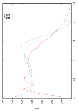
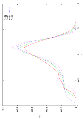
For $D=3$, an almost uniform rigid ball $D^{3}$ is formed, as we can see from Fig. 3. The unit of length is determined from the normalization of the action (19). Its radius is about $1.7$. On the other hand, for $D=4$ the distribution is more like a shell, a three-sphere $S^{3}$ with radius $\sim 1.2$, as is shown in Fig. 3. It is not clear whether or not the thickness of the shell goes to zero at large $N$. We note that since D-brane positions themselves have uncertainty as will be discussed in § 3.3, even if the thickness becomes zero its physical implication is not clear.

3.3 Distribution of the off-diagonal components and validity of the procedure

In this subsection we study the behavior of off-diagonal components and confirm that our criterion discussed in § 3.1 holds for a wide range of distances between D-branes.

First, we should make a few technical observations regarding the distribution of off-diagonal components. We start from observing that the maximally diagonal condition does not fix the gauge completely: the measure for the diagonality (20) is invariant under the $U(1)^{N}$ transformation, generated by $U=diag(e^{i\theta_{1}},\cdots,e^{i\theta_{N}})$. Under this $U(1)^{N}$ transformation diagonal components $X_{ii}$ do not change while off-diagonal components $X_{ij}$ are multiplied by $e^{i(\theta_{i}-\theta_{j})}$. Hence it is natural to study the distribution of the absolute value $|X_{ij}|$. The density function for off-diagonal elements $\rho(|X_{ij}|)$ then acquires the usual volume factor $2\pi|X_{ij}|$ in addition to the Gaussian weight. Because of the overall factor $N$ in the action, it is also convenient to rescale off-diagonal components $X_{ij}$ as $X_{ij}^{new}=\sqrt{N}X_{ij}$, so that $y=|X_{ij}^{new}|$ becomes $O(1)$.

If we neglect the interaction terms in (22) according to our criterion, the statistical distribution of $y$ for fixed value of $\vec{X}_{ii}-\vec{X}_{jj}$ should behave as

$$\rho(y)=2a^{2}y\exp\left(-a^{2}y^{2}\right),$$ (25)

with

$$a=|\vec{X}_{ii}-\vec{X}_{jj}|\equiv d.$$ (26)

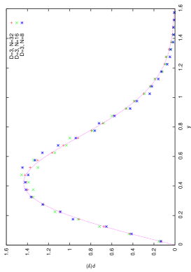
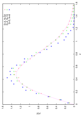
The overall constant is fixed by the normalization $\int dx\rho(x)=1$. We find that (25) provides a good fit in a large region of $|\vec{X}_{ii}-\vec{X}_{jj}|$, see Fig. 5 for example. In general the value of $a$ differs from $d$ but the ratio $a/d$ as a function of $d$ is close to $1$ except for small $d$. This confirms our expectation that when D-branes are far apart, the distribution of off-diagonal elements is the Gaussian following from the first term in (22). At the short distance scale our criterion breaks down. As we will show in § 5, in the supersymmetric case our criterion holds even for shorter distances.

Figure 4: The distribution of off-diagonal components $\rho(y)$, with $1.50\leq d\leq 1.55$, in $D=3$ model. For $N=32$, the ansatz (25) with $a=1.67$ provides a reasonable fit.

Figure 5: The distribution of off-diagonal components $\rho(y)$, with $1.00\leq d\leq 1.05$, in $D=3$ model. For $N=32$, the ansatz (25) with $a=1.51$ provides a reasonable fit. Finite-$N$ corrections are rather large.

Figure 6: $a/d$ vs $d$, $D=3$.

Figure 7: $a/d$ vs $d$, $D=4$.

Figure 8: Distribution of $d$, $D=3$.

Figure 9: Distribution of $d$, $D=4$.

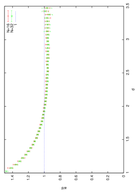
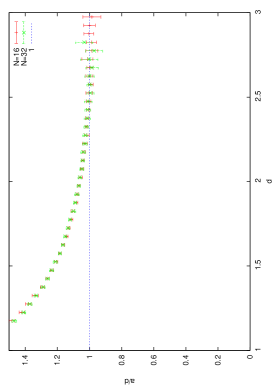
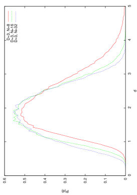
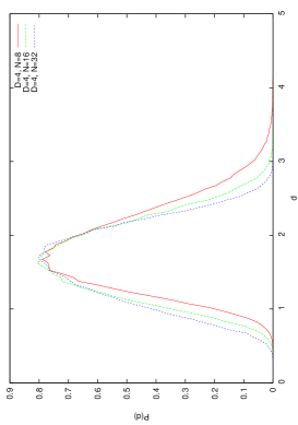
As we can see from Fig. 7 and Fig. 7, (26) approximately holds when $|\vec{X}_{ii}-\vec{X}_{jj}|\gtrsim 1.5$, which is comparable to the radius of the D-brane distribution. This fact strongly suggests that, at this scale, the relative positions of the D-branes can be determined precisely. In Fig. 9 and Fig. 9 we plot the distribution of distances between two points,  $P(d)$, normalized by the condition $\int dxP(x)=1$, which is consistent with the result of [24]. We can see that many pairs of branes are sufficiently separated so that their relative positions can be determined precisely. Thus, even in the bosonic model, resolution for the D-brane position is rather good and the D-brane distribution shown in § 3.2 makes sense. This gives enough motivation to apply the maximal diagonalization procedure to study the BH/BS transition, which will be done in § 4.3.

As we can see by comparing Fig. 5 and Fig. 5, finite-$N$ corrections are larger at the shorter distance scale. This is probably due to the finite-$N$ correction coming from the Faddeev-Popov determinant for the maximally diagonal gauge. We have not evaluated the Faddeev-Popov determinant in full generality. For the simple and important case where only one off-diagonal mode is excited, the Faddeev-Popov determinant can be evaluated and is proportional to $\frac{d^{4}}{4}-\frac{d^{2}z^{2}}{N}+\frac{z^{4}}{3N^{2}}$, where $d=|X_{ii}-X_{jj}|$, $z=\sqrt{|X_{tr}^{1}|^{2}+|X_{tr}^{2}|^{2}}$ and $X_{tr}$ stands for the relevant off-diagonal transverse mode of $X^{new}$. For large $N$, the first term dominates and one can simply neglect the determinant as it only gives a constant factor when considering the distribution of $z$ for fixed $d$. For finite $N$ and small $d$, $z$ spreads to large values and hence the second and the third terms of the determinant should give large contributions.

4 Matrix quantum mechanics and black hole/black string topology change

The action of the bosonic matrix model in $(0+1)$ dimension is

$$S=N\int_{0}^{L}dx\ Tr\left(\frac{1}{2}(DX_{i})^{2}-\frac{1}{4}[X_{i},X_{j}]^{2}\right).$$ (27)

Here $D=\partial_{x}-i[A,\ \cdot\ ]$ is the gauge covariant derivative and $X_{i}(i=1,\cdots,d_{s})$ are adjoint scalars. When $d_{s}=9$, this model is the high-temperature limit of $(1+1)$-dimensional maximal super Yang-Mills theory. (We have absorbed factors such as $\lambda T_{H}$ in (5) by redefining fields and the coordinate $x$.)

As is discussed in § 2, this model is related to the black hole/black string transition. We begin with the study of its phase structure in § 4.1. Next we generalize the maximal diagonalization procedure to higher dimensions in § 4.2. Then in § 4.3 we apply this procedure to the matrix quantum mechanics and see the topology change. We find that, at the transition [7] corresponding to the BH/BS transition [6], there is a topology change which strikingly resembles the counterpart on the gravity side [16].

4.1 Phase structure of matrix quantum mechanics

In this section we study the phase structure of the bosonic matrix quantum mechanics. The argument is parallel to that in [23]; the only difference is in the number of scalars, $d_{s}$.

As is well-known, the model has a global $U(1)$ symmetry, multiplying the Wilson loop $TrW\equiv\frac{1}{N}Tr{\rm P}\exp(i\int_{0}^{L}dxA_{x})$, winding on the compactified direction, by a phase factor. This symmetry can be broken in the large-$N$ limit. In order to detect the breakdown of this symmetry, we should measure $\langle|TrW|\rangle$ rather than $\langle TrW\rangle$, because the overall phase factor is not fixed at finite-$N$. As shown in [7, 23] the global $U(1)$ symmetry is broken when $L$ is small. To study the detail of the transition, it is better to look at eigenvalues of $W$ rather than $TrW$ itself. Because $W$ is unitary, its eigenvalues are written as $e^{i\theta}$, where $-\pi\leq\theta\leq\pi$. We study the distribution of the phases $\rho(\theta)$. Note that we fix the overall phase factor such that $TrW$ becomes real. By looking at the distribution $\rho(\theta)$, it was found that there are two successive transitions at $L=L_{1}$ and $L=L_{2}<L_{1}$ [23]. Above $L=L_{1}$ the phase distribution is uniform, $\rho(\theta)=1/(2\pi)$, and hence the $U(1)$ symmetry is not broken, $\langle|TrW|\rangle=0$. Therefore, the theory is volume independent [32, 33] in this region. Below $L=L_{1}$ the distribution is not uniform. For $L_{2}<L<L_{1}$, $\rho(\theta)$ is not a constant and is non-zero everywhere. Below $L=L_{2}$ the distribution has a gap (i.e. $\rho(\theta)$ becomes zero at a certain value of $\theta$). It has been observed that the phase distribution below $L=L_{1}$ can be fitted [23] by an expression used for the Gross-Witten model [34], which is,

$$\frac{1}{2\pi}\left(1+\frac{2}{\kappa}\cos\theta\right)\qquad(\kappa\geq 2)$$ (28)

for ungapped phase $L_{2}\leq L<L_{1}$ and

$$\frac{2}{\pi\kappa}\cos\frac{\theta}{2}\sqrt{\frac{\kappa}{2}-\sin^{2}\frac{\theta}{2}}\qquad(\kappa<2)$$ (29)

for gapped phase $L<L_{2}$.

In the following we show the results for $d_{s}=2$ and $d_{s}=3$. In Figure 10 we show the phase distribution for $d_{s}=2$ when $L$ is very close to $L_{2}$. We find the gap emerges at $L_{2}\simeq(1.3)^{-1}\simeq 0.8$. This transition is of second order [23]. We note that the corresponding transition in the Gross-Witten model is of third order.

Figure 10: Distribution of the Wilson line phase near transition point. $d_{s}=2,N=32,\Lambda=12$.

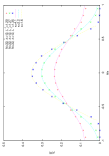
In order to determine the value of $L_{1}$, we utilize the $L$-dependence of $\kappa$. For $N=32$ and $\Lambda=12$, $\kappa^{-1}$ can be fitted by the straight line, $\kappa^{-1}\simeq 3.3L^{-1}-3.7$, at $1.2\leq L^{-1}\leq 1.26$, and we can estimate the value of $L_{1}$, where $\kappa$ becomes infinity, to be around $(1.12)^{-1}\simeq 0.89$. To determine the order of the transition, we fit the quantity $\int-\frac{1}{N}\langle Tr[X_{i},X_{j}]^{2}\rangle dx\propto\frac{\partial}{\partial L}\log Z$, where $Z$ is the partition function, by an ansatz

$$\int-\frac{1}{N}\langle Tr[X_{i},X_{j}]^{2}\rangle dx=a(L^{-1}-1.12)^{p}+C,$$ (30)

where $C\simeq 0.94$ is the value for $L\geq L_{1}$. Then, for the data at $1.2\leq L^{-1}\leq 1.26$ for $N=32,\Lambda=12$, we perform a two parameter fit with respect to $a$ and $p$, and we obtain $p\simeq 2.0$, which means that the transition is of third order.

For $d_{s}=3$, the behavior of the eigenvalues are qualitatively the same and, in this case, we find $L_{1}\simeq(0.93)^{-1}\simeq 1.08$ and $L_{2}\simeq(1.1)^{-1}\simeq 0.9$.

4.2 Maximal diagonalization for matrix quantum mechanics: T-dual case

As explained in § 2, we should go to the T-dualized picture in order to see the black hole/black string transition. In the matrix model, we should use Taylor’s T-duality for Yang-Mills theories [5], which we shall briefly recall here. The starting point is the zero-dimensional bosonic YM,

$$S_{0d}=-\frac{1}{4}Tr[X^{P},X^{Q}]^{2},$$ (31)

where $P,Q=(0,i)=(0;1,\cdots,d_{s})$. The next step is to divide $X^{P}$ into infinite number of blocks with the size $N$, $N^{1/4}X_{mn}^{P}$; we obtain

$$S=-\frac{N}{4}tr\left(X_{mq}^{P}X_{qn}^{Q}-X_{mq}^{Q}X_{qn}^{P}\right)\left(X_{nr}^{P}X_{rm}^{Q}-X_{nr}^{Q}X_{rm}^{P}\right),$$ (32)

where $tr$ is a trace in each block and the summation over $m,n,\cdots$ is assumed. Then we impose the compactification constraint,

$$X_{mn}^{i} = X_{(m-1)(n-1)}^{i},$$

$$X_{mn}^{0} = X_{(m-1)(n-1)}^{0}\qquad(m\neq n),$$

$$X_{nn}^{0} = X_{(n-1)(n-1)}^{0}+2\pi R\cdot\textbf{1}.$$ (33)

Under this constraint, the action (32) should be divided by the (infinite) number of copies and re-expressed in terms of $X_{n}^{P}\equiv X_{n0}^{P}$. For $n\neq 0$ these matrices represent open strings between D-branes with the winding number $n$. For $n=0$, diagonal components represent positions of D-branes and off-diagonal components represent open strings with no winding. By T-duality, the winding number is translated to the KK momentum: we choose variables after performing the T-dual transformation as

$$A_{x}\equiv\sum_{n}e^{2\pi inxR}X_{n}^{0},\qquad Y^{i}\equiv\sum_{n}e^{2\pi inxR}X_{n}^{i}.$$ (34)

Then, the action becomes

$$S_{1d}=NR\int_{0}^{R^{-1}}dx\ tr\left(\frac{1}{2}(D_{x}Y_{i})^{2}-\frac{1}{4}[Y_{i},Y_{j}]^{2}\right).$$ (35)

Then, by rescaling

$$Y^{(new)}=R^{1/3}Y^{(old)},\qquad A_{x}^{(new)}=R^{1/3}A_{x}^{(old)},\qquad x^{(new)}=R^{-1/3}x^{(old)}$$ (36)

we obtain

$$S_{1d}=N\int_{0}^{R^{-4/3}}dx\ tr\left(\frac{1}{2}(D_{x}Y_{i})^{2}-\frac{1}{4}[Y_{i},Y_{j}]^{2}\right).$$ (37)

From these rules, we learn that open strings between different D-branes in the T-dualized picture correspond to the non-constant modes and the off-diagonal elements in the one-dimensional YM. Hence, it is natural to minimize non-constant modes and off-diagonal elements. We note that we should distinguish here between the minimization of off-diagonal components (and non-constant modes) and the maximization of diagonal components, as one cannot use the conservation of the matrix norm by unitary transformations (21). (We use the term “maximal diagonalization” throughout this paper although it is a slight abuse of the terminology. ) Actually, the minimization procedure gives sensible results, as we will see, whereas the maximization procedure turns out to give pathological results. One way to understand the difference is to note that the measure for the size of off-diagonal (and non-constant) elements and diagonal elements are positive. For the minimization procedure, this serves as a lower bound to stabilize the procedure, whereas the maximization procedure is more susceptible to pathology because of the absence of an upper bound.

Another technical issue is that, to look at the distribution of branes, we have to take care of the effect of the translational symmetry, and fix the origin for branes. To fix the origin for a noncompact direction, we simply take $X$ to be traceless. To fix the origin of the $S^{1}$ direction, we fix the global $U(1)$ symmetry so that the Wilson loop $Tr{\rm P}\exp(i\int dxA_{x}(x))$ becomes real and positive [23].

Our simulation is based on the non-lattice technique [26]. We generate configurations consisting of the gauge field in the static-diagonal gauge

$$A_{x}=\frac{1}{L}\cdot diag(\alpha_{1},\cdots,\alpha_{N}),\qquad L=R^{-4/3},$$ (38)

and Fourier modes of adjoint scalars

$$\tilde{Y}_{i}(p)\ (p=-\Lambda,\cdots,\Lambda).$$ (39)

Because the coordinate basis is more convenient for maximal diagonalization, we introduce $2\Lambda+1$ lattice sites

$$x=-\frac{\Lambda}{2\Lambda+1}L,\ \cdots,\ 0,\ \cdots,\ \frac{\Lambda}{2\Lambda+1}L,$$ (40)

and perform the Fourier transformation

$$Y_{i}(x)=\sum_{p=-\Lambda}^{\Lambda}e^{2\pi ipx/L}\tilde{Y}_{i}(p).$$ (41)

The gauge field is mapped to the unitary link variable as

$$U(x)=diag(e^{i\alpha_{1}/(2\Lambda+1)},\cdots,e^{i\alpha_{N}/(2\Lambda+1)})$$ (42)

After performing the unitary transformation in the coordinate basis to maximally diagonalize, we have to go back to the momentum basis to use the T-dualized picture.

From the above considerations, it follows that one should minimize

$$\frac{2\Lambda+1}{L^{2}}\sum_{x}Tr\left(2-U(x)-U^{\dagger}(x)\right)+\sum_{i}\left[\frac{1}{L^{2}}{\rm Re}\left\{\sum_{x}\left(U_{ii}(x)-1\right)\right\}^{2}-\frac{1}{(2\Lambda+1)^{2}}\left(\sum_{x}Y_{ii}(x)\right)^{2}\right].$$ (43)

The detailed derivation is given in Appendix A.

4.3 Black hole/black string topology change

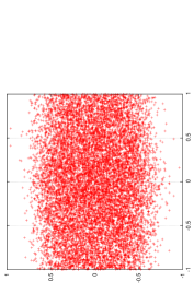
In this section we show the D-brane distribution, obtained by using the maximal diagonalization procedure introduced in the previous subsection. The off-diagonal components behaves similarly to the zero-dimensional model studied in § 3.3 and hence the distribution is meaningful. In Figure 13, 13 and 13 we plot diagonal components after the maximal diagonalization for the $d_{s}=2$ model. The x-axis represents the compactified direction and two edges $\pm 1$ should be identified. (In these plots we have rescaled the coordinates so that the period of the compactified direction becomes $2$.) The y-axis represents the $X_{1}$ direction. The $X_{2}$ direction is projected out.

When the radius $R$ in the T-dual picture is small (i.e. $L$ large) they form a uniform string, as we can see from Figure 13. If $R$ becomes large, at some point the string begins to pinch; see Figure 13. We may call it as the nonuniform string. Finally it is pinched off completely and becomes a squashed ball, as shown in Figure 13. These shapes are strikingly similar to the black string and the black hole in gravity side [16]. As we increase $R$ further, we have found that the distribution exhibits $SO(d_{s}+1)$ symmetry, as expected. If one does not apply the maximal diagonalization and just plots diagonal components resulting from a Monte-Carlo simulation (in the static-diagonal gauge), these gradual change of the geometry is almost completely obscured. In particular, one cannot see the recovery of the spherical symmetry for large $R$.

We have also studied the $d_{s}=3$ model, and found that the shapes of the bound states look similar. The difference is in their internal structures: for $d_{s}=2$ the bound state is uniformly filled ($D^{2}\times S^{1}$ for the black string phase and $D^{3}$ for the black hole phase), and for $d_{s}=3$ the distribution is shell-like ($S^{2}\times S^{1}$ for the black string phase and $S^{3}$ for the black hole phase).

Figure 11: Distribution of diagonal components for $d_{s}=2,N=16,\Lambda=8,L^{-1}=0.5$. The “uniform black string” phase.

Figure 12: Distribution of diagonal components for $d_{s}=2,N=16,\Lambda=8,L^{-1}=1.2$. The “nonuniform black string” phase.

Figure 13: Distribution of diagonal components for $d_{s}=2,N=16,\Lambda=8,L^{-1}=1.5$. The “black hole” phase.

5 Supersymmetric matrix models

In this section we show preliminary simulation results on a supersymmetric matrix quantum mechanics. We adopt the non-lattice Euclidean path-integral method [26]. A Hamiltonian formulation can be found in [35], and a mean field approximation is studied in [36]. As explained in § 2, at low temperature the maximally symmetric model (17) describes the black 0-brane in IIA supergravity. Here we study a simpler model, the four-supercharge analogue of (17) :

$$S=N\int_{0}^{1/T}dt\ Tr\left(\frac{1}{2}(D_{t}X_{I})^{2}-\frac{1}{4}[X_{I},X_{J}]^{2}+\bar{\psi}D_{t}\psi-\bar{\psi}\sigma^{I}[X_{I},\psi]\right),$$ (44)

which is obtained from four-dimensional ${\cal N}=1$ SYM through the dimensional reduction. Here $I,J$ runs through $1,2$ and $3$, $\sigma^{I}$ are Pauli matrices, and $\psi_{\alpha}\ (\alpha=1,2)$ are $N\times N$ complex fermionic matrices. This model does not suffer from the sign problem and the simulation cost is less expensive, while we expect its behavior should at least qualitatively similar to that of (17). To consider the finite temperature system we have to impose the anti-periodic boundary condition (a.p.b.c.) to the fermion. However, as pointed out in [17], with the a.p.b.c. the system with small $N$ and finite $T$ has an instability (eigenvalues of $X_{I}$ run to infinity), which makes the computation heavy as we need to take $N$ to be reasonably large. This lead us to adopt the periodic boundary condition (p.b.c.), as the p.b.c. and a.p.b.c should be the same in the $T\to 0$ limit which we are interested in.

Because the compactified direction is now temporal and the T-duality transformation is not performed, the maximal diagonalization procedure introduced in § 4.2 is not adequate. Rather, we maximize $\sum_{I}\sum_{p}\int dt\left(X^{I}_{pp}\right)^{2}$, that is, we maximally diagonalize scalars at each time slice.  Numerically, at $N=6$, the diagonal components we find are distributed like a ball. To determine the shape of the distribution reliably, it is also necessary to study larger $N$ and see the $N$-dependence. We would like to report on this issue in a future work.

We should also introduce a slightly different criterion for determining the validity of the maximal diagonalization. We again regard the diagonal and off-diagonal elements to be the position of the D0-branes and open strings, respectively. Our criterion is again to see when we can neglect higher order interaction terms (and accordingly can think of off-diagonal elements as dynamically insignificant). If interaction terms are negligible, and the diagonal elements are slowly-varying compared to the off-diagonal elements, each off-diagonal mode behaves as a harmonic oscillator. Quanta of this harmonic oscillator correspond to open strings and have energies proportional to their lengths. As we are interested in the low temperature limit, we furthermore require that the open string is not excited at all, the wave function being of the Gaussian form. This is the minimal non-commutativity; off diagonal components cannot vanish because of the zero point oscillation.

Indeed, we find that the distribution of $y\equiv\sqrt{N}|X_{ij}|$ can be fitted by the probability distribution function for the zero-point oscillation

$$\rho(y)=4aye^{-2ay^{2}}$$ (45)

in a wide region, and $a$ is very close to $d\equiv|\vec{X}_{ii}(t)-\vec{X}_{jj}(t)|$. In Fig. 15 we plot $a/d$ against $d$. In Fig. 15, we plotted $a/d$ for fixed $d$ against $T$. At short distance, the data begins to depart from the ansatz (45). We suspect the reason to be corrections in the Faddeev-Popov determinant, which are not negligible for finite $N$ as we have seen in § 3.3; to study $d\lesssim 1.5$ reliably, we have to take larger $N$.

The applicability of the ansatz (45) is at least an indication of the validity of the assumption that the D0-branes (diagonal components) are more slowly-varying than the open strings (off-diagonal components). We note that this assumption is crucial for previous studies [37, 38] for D-brane bound states, using various analytic and approximate methods. For another approach to bound states, see [39, 40, 41, 42]. For a discussion of bound states for the zero-dimensional matrix model, see [43].

Figure 14: The ratio $a/d$ in 4 SUSY matrix quantum mechanics is plotted against $d$.

Figure 15: Plot of $a/d$ versus $T$ at $d=1.55,2.05$ and $2.55$ in 4 SUSY matrix quantum mechanics.

Figure 16: The ratio $a/d$ in the bosonic matrix quantum mechanics with 3 scalars is plotted against $d$.

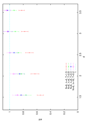
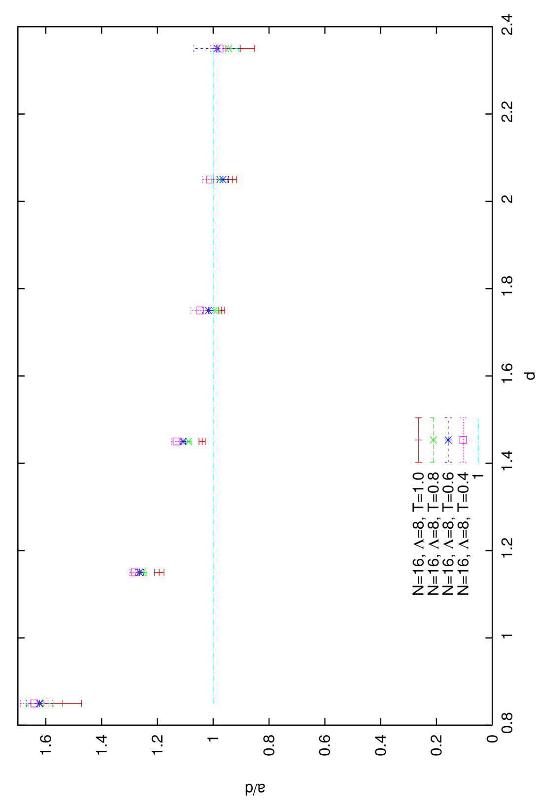
From these plots, we can see that the notion of the D-brane distribution becomes better at smaller $T$.  A more interesting possibility suggested by these plots is that $a/d=1$ holds for any $d$ at $T=0$ in the planar limit. Let us elaborate on this possibility and the general tendency that our criterion holds better at lower temperature. As we are taking the $T\rightarrow 0$ limit, it is expected that the off-diagonal elements are in ground states, not in excited states. What is surprising is that the effect of the higher-order interaction terms seems to be negligible even for small distances between D-branes, because for small distances the width of the wave function (for each off-diagonal element) is large and therefore one expects that the higher order terms in the action also contribute. The fact that this absence of the effect of interaction terms occurs for supersymmetric models and not for bosonic models suggests that this might be a consequence of the familiar cancellation between bosonic and fermionic degrees of freedom. It is a very interesting problem to understand the mechanism of this phenomenon. Of course, to obtain a rigid conclusion we also have to study the model more thoroughly for larger $N$ and smaller $T$. We would like to report on these issues in a future publication.

It might be worthwhile to compare this with an approach [45, 46], centering around the Berenstein’s conjecture [45] on the strongly coupled ${\cal N}=4$ SYM on ${\mathbb{R}}\times S^{3}$. As this approach focuses on dynamics of the diagonal elements, neglecting that of the off-diagonal elements, it is closely related to the themes of this paper. In this approach one has an additional dimensionful parameter, the mass for scalar fields, originating from the curvature of the $S^{3}$. Because of this, under a crucial assumption explained below, the strong coupling limit implies very large mass terms for the off-diagonal elements. This in turn implies that the width of the wave function (or the Gaussian) is very small, which automatically validates the neglection of interaction terms. This is similar to, but has a crucial difference from what seems to be happening in our model: for our models, the widths of the Gaussian distributions are generated dynamically, and are finite instead of vanishingly small. Nonetheless, also in our model higher order interaction terms seem not to have effect in dynamics in the low temperature regime.

The assumption mentioned above, underlying the analysis of ${\cal N}=4$ SYM on ${\mathbb{R}}\times S^{3}$, is that the typical length scale for distances between D-branes should be determined basically by the additional dimensionful parameter (the size of $S^{3}$) and should not depend too much on the coupling constant, which is also dimensionful. In [29], a mechanism for explaining this behavior is proposed, which is also closely related to the behavior we find numerically for $T\rightarrow 0$. The mechanism is based on an instability of the D-brane bound state in finite-$N$ supersymmetric matrix models (without mass-terms for scalars), where distances between D-branes become arbitrarily large.  In the presence of the mass-term for scalars, there would be a competition between this instability and the attractive force from the mass-term. The balance between these competing effects would be achieved at the point where the coordinates of D-branes take values of the order of the length scale determined by the mass-term, thus validating the assumption. One can partially justify the existence of this instability by using the one-loop approximation [27, 48] which is valid once the distances between D-branes become large. Our numerical results suggest that one might be able to extend this result even for shorter distances.

As also noted above, the low temperature behavior we find numerically, namely the absence of the effect of higher order interaction terms for a rather short distance scale, suggests that physics in the low temperature regime might be understood by an one-loop approximation. We hope that our numerical results provide a guide to such an improved perturbation theory.

6 Conclusion and Discussions

In this paper we have proposed a simple procedure to determine the shape of the D-brane bound state from super Yang-Mills theories. The strategy is to maximally diagonalize the matrices representing the collective coordinates of the D-branes. We have introduced a criterion which determines when the notion of this D-brane position makes sense. We have tested the use of these ideas by Monte-Carlo simulations. As the maximally supersymmetric SYM are computationally hard, we have studied simpler models– zero-dimensional and one-dimensional bosonic YM and one-dimensional SYM with four supercharges. In the bosonic models, the criterion is satisfied for the typical distance scale between D-branes. The size of the whole distribution of D-branes is a few times larger than this length scale below which one cannot talk about D-brane positions. This is natural because a theory of quantum gravity would have a minimal length scale and very hot black holes, presumably described by the bosonic matrix models, would be objects of the size comparable to this scale. We also observed the topology change of the D-brane distribution corresponding to the BH/BS transition, by combining the above procedure and the T-duality prescription for YM. In the supersymmetric model, the notion of the D-brane position seems to be precise even at shorter distance scales.

There are many future directions. Most straightforward one is to try to understand the gauge/gravity correspondence, and furthermore, to study the black hole physics via the correspondence. We have already seen the analogue of the BH/BS transition in the bosonic model. It is in principle straightforward to repeat the similar analysis for (1+1)-dimensional SYM. The lattice formulation for (1+1)-dimensional SYM has been developed recently [49] and already Monte-Carlo simulations have been performed for four-supercharge $SU(2)$ gauge theory [50]. By carrying out simulations for larger $N$ and larger supercharges the BH/BS transition can be directly studied. At low but finite temperature, we expect to see even the stringy correction to the transition. As we have reviewed in § 2, the pattern of the phase transition changes at intermediate temperature – although there are two successive phase transitions at high temperature, the dual gravity analysis predicts there is only one transition at low temperature. It should be possible to see how high and low temperature regions are interpolated. At present it is still numerically challenging, but will be possible in near future. Also it will be interesting to study (1+2)- and (1+3)-dimensional SYM compactified on torus, which are expected to have richer phase diagrams [51, 52]. A generalization to curved spacetime is also interesting. For this purpose, the T-duality procedure on curved spacetime [53] and a construction [54] of the four-dimensional ${\cal N}=4$ planar SYM on $S^{3}$ from the BMN matrix model [55] might be useful.

Another interesting direction is to apply our techniques to study noncommutative spaces and supermembranes [56]. As we can see from Figure 1, the maximal diagonalization procedure can be a powerful tool to read off the shape of noncommutative manifolds. In this case, off-diagonal components are very small, although non-zero, and the shape is determined precisely. For example, we might be able to see the shape of the higher-genus membranes (fuzzy surfaces) constructed along the line of [57]. For the case of membranes, the embedding of the topology in the matrices has been discussed in [31], and it will be interesting to see the relation with the current approach. The study of the ground state of the matrix models for string/M theory [56, 28, 58], which presumably is associated with a different type of large $N$ limit than the planar limit, is also an important direction.

We wish to stress that the rather high applicability of the Gaussian distribution for the off-diagonal elements are, although natural, far from trivial. This Gaussian behavior suggests an existence of an improved perturbation theory (presumably some kind of mean-field approximations incorporating the information of the distribution of the diagonal elements) and its validity at the one-loop level. Usually one does not expect that the perturbation theory should be useful, as the ’t Hooft coupling constant $\lambda$ is dimensionful and we cannot compete it with the kinetic term for the mass-less case we are interested in. (For matrix models with a mass-term the ratio between the mass and the ’t Hooft coupling constant gives a good estimate about the applicability of the perturbation scheme. ) It is also interesting that the validity of the perturbation is associated with each pair of D-branes rather than with the whole configuration. As shown in § 5 for the supersymmetric matrix quantum mechanics at low temperature, the one-loop approximation is valid for very short distance scales, and the one-loop effective action provides a precise description. This observation may support a proposal in [21], that a critical exponent $2.8$ of the energy density of the black hole, $\frac{E}{N^{2}}\sim 7.4T^{2.8}$, predicted by using the supergravity dual [3], might be understood from the one-loop effective action [60]. It will be nice if we can reproduce not only the exponent but also the overall factor $7.4$. More importantly, the distribution of D-branes given by our method should correspond somehow to the metric of the black hole. Clarification of this correspondence would give us a good clue to understand the gauge/gravity duality directly. We hope that our method provides a useful mean to organize data and extract physics from it.

Acknowledgments

The authors would like to thank O. Aharony, J. Hoppe, H. Kawai, Y. Kimura, T. McLoughlin, L. Mannelli, J. Nishimura, T. Nishioka, N. Obers, D. Robles-Llana, S. Theisen and D. Yamada for discussions and comments. T. A. and T. H. would like to thank the Japan Society for the Promotion of Science for financial support. M. H. would like to thank also for Niels Bohr Institute, Albert Einstein Institute, University of Tokyo Hongo and RIKEN Nishina Center for hospitality during his stay. H. S. would like to thank IHES and University of Tokyo Komaba for hospitality. H. S. is supported by the grant SFB647 “Raum-Zeit-Materie”. The numerical computation in this work were carried out at the Yukawa Institute Computer Facility.

Appendix A Details of the maximal diagonalization in matrix quantum mechanics in T-dual picture

In this appendix we explain why we should minimize (43) in the maximal diagonalization procedure.

Because

$$U(x)={\rm P}\exp\left(i\int_{x}^{x+a}dx^{\prime}A(x^{\prime})\right)\simeq e^{iaA(x)},\qquad U(x)+U^{\dagger}(x)\simeq 2-a^{2}A(x)^{2},$$ (46)

we have

$$\frac{1}{a^{2}}\sum_{x}Tr\left(2-U(x)-U^{\dagger}(x)\right)\simeq\sum_{x}TrA(x)^{2}=(2\Lambda+1)\sum_{p}\sum_{ij}\left|\tilde{A}_{ij}(p)\right|^{2}.$$ (47)

Here $a=L/(2\Lambda+1)$ is the lattice spacing. Also, the zero-mode of diagonal components can be approximated as

$$\tilde{A}_{ii}(0)=\frac{1}{L}\sum_{x}aA_{ii}(x)=\frac{-i}{L}\sum_{x}\left(U_{ii}(x)-1\right).$$ (48)

Therefore, the contribution to the quantity we wish to minimize from the off-diagonal and nonzero modes can be written as

$$\sum_{p}\sum_{ij}\left|\tilde{A}_{ij}(p)\right|^{2}-\tilde{A}_{ii}(0)^{2}\simeq\frac{2\Lambda+1}{L^{2}}\sum_{x}Tr\left(2-U(x)-U^{\dagger}(x)\right)+\frac{1}{L^{2}}\sum_{i}{\rm Re}\left\{\sum_{x}\left(U_{ii}(x)-1\right)\right\}^{2}.$$ (49)

Expressions for adjoint scalars are also similar. We have

$$\sum_{x}TrY(x)^{2}=(2\Lambda+1)\sum_{p}\sum_{ij}\left|\tilde{Y}_{ij}(p)\right|^{2}$$ (50)

and

$$\tilde{Y}(0)=\frac{1}{2\Lambda+1}\sum_{x}Y(x),$$ (51)

and hence the total contribution from adjoint scalar is

$$\sum_{p}\sum_{ij}\left|\tilde{Y}_{ij}(p)\right|^{2}-\sum_{i}\left|\tilde{Y}_{ii}(0)\right|^{2}=\frac{1}{2\Lambda+1}\sum_{x}TrY(x)^{2}-\sum_{i}\left(\frac{1}{2\Lambda+1}\sum_{x}Y_{ii}(x)\right)^{2}.$$ (52)

As $TrY(x)^{2}$ is gauge invariant, we need to evaluate only the second term. In summary, we should minimize

$$\frac{2\Lambda+1}{L^{2}}\sum_{x}Tr\left(2-U(x)-U^{\dagger}(x)\right)+\sum_{i}\left[\frac{1}{L^{2}}{\rm Re}\left\{\sum_{x}\left(U_{ii}(x)-1\right)\right\}^{2}-\frac{1}{(2\Lambda+1)^{2}}\left(\sum_{x}Y_{ii}(x)\right)^{2}\right].$$ (53)

Note that first term does not appear if we perform the maximization of diagonal components instead of the minimization of off-diagonal components.

References

- [1] E. Witten, “Bound states of strings and p-branes,” Nucl. Phys. B 460 (1996) 335 [arXiv:hep-th/9510135].
- [2] J. M. Maldacena, “The large N limit of superconformal field theories and supergravity,” Adv. Theor. Math. Phys. 2, 231 (1998) [Int. J. Theor. Phys. 38, 1113 (1999)] [arXiv:hep-th/9711200].
- [3] N. Itzhaki, J. M. Maldacena, J. Sonnenschein and S. Yankielowicz, “Supergravity and the large N limit of theories with sixteen supercharges,” Phys. Rev. D 58, 046004 (1998) [arXiv:hep-th/9802042].
- [4] T. Hotta, J. Nishimura and A. Tsuchiya, “Dynamical aspects of large N reduced models,” Nucl. Phys. B 545 (1999) 543; [arXiv:hep-th/9811220].
- [5] W. Taylor, “D-brane field theory on compact spaces,” Phys. Lett. B 394, 283 (1997); [arXiv:hep-th/9611042].
- [6] R. Gregory and R. Laflamme, “Black strings and p-branes are unstable,” Phys. Rev. Lett. 70, 2837 (1993); [arXiv:hep-th/9301052].
- [7] O. Aharony, J. Marsano, S. Minwalla and T. Wiseman, “Black hole - black string phase transitions in thermal 1+1 dimensional supersymmetric Yang-Mills theory on a circle,” Class. Quant. Grav. 21 (2004) 5169 [arXiv:hep-th/0406210]. O. Aharony, J. Marsano, S. Minwalla, K. Papadodimas, M. Van Raamsdonk and T. Wiseman, “The phase structure of low dimensional large N gauge theories on tori,” JHEP 0601, 140 (2006); [arXiv:hep-th/0508077].
- [8] L. Susskind, “Matrix theory black holes and the Gross Witten transition,” hep-th/9805115.
- [9] J. L. F. Barbon, I. I. Kogan and E. Rabinovici, “On stringy thresholds in SYM/AdS thermodynamics,” Nucl. Phys. B 544, 104 (1999); hep-th/9809033.
- [10] M. Li, E. J. Martinec and V. Sahakian, “Black holes and the SYM phase diagram,” Phys. Rev. D 59, 044035 (1999); hep-th/9809061.
- [11] E. J. Martinec and V. Sahakian, “Black holes and the SYM phase diagram. II,” Phys. Rev. D 59, 124005 (1999); hep-th/9810224.
- [12] T. Harmark and N. A. Obers, “New phases of near-extremal branes on a circle,” JHEP 0409, 022 (2004); hep-th/0407094.
- [13] B. Kol, “The phase transition between caged black holes and black strings: A review,” Phys. Rept. 422, 119 (2006); hep-th/0411240. T. Harmark, V. Niarchos and N. A. Obers, “Instabilities of black strings and branes,” Class. Quant. Grav. 24, R1 (2007); hep-th/0701022.
- [14] H. Kawai and T. Suyama, “AdS/CFT Correspondence as a Consequence of Scale Invariance,” Nucl. Phys. B 789 (2008) 209 [arXiv:0706.1163 [hep-th]]. T. Azeyanagi, M. Hanada, H. Kawai and Y. Matsuo, “Worldsheet Analysis of Gauge/Gravity Dualities,” arXiv:0812.1453 [hep-th].
- [15] G. T. Horowitz and A. Strominger, “Black strings and P-branes,” Nucl. Phys. B 360, 197 (1991).
- [16] H. Kudoh and T. Wiseman, “Connecting black holes and black strings,” Phys. Rev. Lett. 94, 161102 (2005) [arXiv:hep-th/0409111].
- [17] K. N. Anagnostopoulos, M. Hanada, J. Nishimura and S. Takeuchi, “Monte Carlo studies of supersymmetric matrix quantum mechanics with sixteen supercharges at finite temperature,” Phys. Rev. Lett. 100 (2008) 021601; arXiv:0707.4454 [hep-th].
- [18] S. Catterall and T. Wiseman, “Black hole thermodynamics from simulations of lattice Yang-Mills theory,” Phys. Rev. D 78, 041502 (2008) [arXiv:0803.4273 [hep-th]].
- [19] M. Hanada, A. Miwa, J. Nishimura and S. Takeuchi, “Schwarzschild radius from Monte Carlo calculation of the Wilson loop in supersymmetric matrix quantum mechanics,” arXiv:0811.2081 [hep-th].
- [20] M. Hanada, Y. Hyakutake, J. Nishimura and S. Takeuchi, “Higher derivative corrections to black hole thermodynamics from supersymmetric matrix quantum mechanics,” arXiv:0811.3102 [hep-th].
- [21] A. V. Smilga, “Comments on thermodynamics of supersymmetric matrix models,” arXiv:0812.4753 [hep-th].
- [22] R. A. Janik and J. Wosiek, “Towards the matrix model of M-theory on a lattice,” Acta Phys. Polon. B 32, 2143 (2001) [arXiv:hep-th/0003121].
- [23] N. Kawahara, J. Nishimura and S. Takeuchi, “Phase structure of matrix quantum mechanics at finite temperature,” JHEP 0710, 097 (2007) arXiv:0706.3517 [hep-th].
- [24] J. Ambjorn, K. N. Anagnostopoulos, W. Bietenholz, T. Hotta and J. Nishimura, “Large N dynamics of dimensionally reduced 4D SU(N) super Yang-Mills theory,” JHEP 0007, 013 (2000) [arXiv:hep-th/0003208].
- [25] W. Krauth, H. Nicolai and M. Staudacher, “Monte Carlo approach to M-theory,” Phys. Lett. B 431 (1998) 31 [arXiv:hep-th/9803117].
- [26] M. Hanada, J. Nishimura and S. Takeuchi, “Non-lattice simulation for supersymmetric gauge theories in one dimension,” Phys. Rev. Lett. 99 (2007) 161602; arXiv:0706.1647 [hep-lat].
- [27] S. Catterall and T. Wiseman, “Towards lattice simulation of the gauge theory duals to black holes and hot strings,” JHEP 0712 (2007) 104; arXiv:0706.3518 [hep-lat].
- [28] T. Banks, W. Fischler, S. H. Shenker and L. Susskind, “M theory as a matrix model: A conjecture,” Phys. Rev. D 55, 5112 (1997) [arXiv:hep-th/9610043].
- [29] D. E. Berenstein, M. Hanada and S. A. Hartnoll, “Multi-matrix models and emergent geometry,” arXiv:0805.4658 [hep-th].
- [30] K. Hashimoto, “The shape of non-Abelian D-branes,” JHEP 0404, 004 (2004) [arXiv:hep-th/0401043].
- [31] H. Shimada, “Membrane topology and matrix regularization,” Nucl. Phys. B 685, 297 (2004) [arXiv:hep-th/0307058].
- [32] T. Eguchi and H. Kawai, “Reduction Of Dynamical Degrees Of Freedom In The Large N Gauge Theory,” Phys. Rev. Lett. 48 (1982) 1063.
- [33] R. Narayanan and H. Neuberger, “Large N reduction in continuum,” Phys. Rev. Lett. 91, 081601 (2003); [arXiv:hep-lat/0303023]. J. Kiskis, R. Narayanan and H. Neuberger, “Does the crossover from perturbative to nonperturbative physics in QCD become a phase transition at infinite N?,” Phys. Lett. B 574, 65 (2003); [arXiv:hep-lat/0308033].
- [34] D. J. Gross and E. Witten, “Possible Third Order Phase Transition In The Large N Lattice Gauge Theory,” Phys. Rev. D 21, 446 (1980). S. R. Wadia, “N = Infinity Phase Transition In A Class Of Exactly Soluble Model Lattice Gauge Theories,” Phys. Lett. B 93, 403 (1980).
- [35] J. Wosiek, “Spectra of supersymmetric Yang-Mills quantum mechanics,” Nucl. Phys. B 644, 85 (2002) [arXiv:hep-th/0203116].
- [36] D. N. Kabat, G. Lifschytz and D. A. Lowe, “Black hole thermodynamics from calculations in strongly coupled gauge theory,” Int. J. Mod. Phys. A 16, 856 (2001) [Phys. Rev. Lett. 86, 1426 (2001)] [arXiv:hep-th/0007051].
- [37] U. H. Danielsson, G. Ferretti and B. Sundborg, “D-particle Dynamics and Bound States,” Int. J. Mod. Phys. A 11, 5463 (1996) [arXiv:hep-th/9603081]. D. N. Kabat and P. Pouliot, “A Comment on Zero-brane Quantum Mechanics,” Phys. Rev. Lett. 77, 1004 (1996) [arXiv:hep-th/9603127]. M. R. Douglas, D. N. Kabat, P. Pouliot and S. H. Shenker, “D-branes and short distances in string theory,” Nucl. Phys. B 485, 85 (1997) [arXiv:hep-th/9608024].
- [38] V. G. Kac and A. V. Smilga, “Normalized vacuum states in N = 4 supersymmetric Yang-Mills quantum mechanics with any gauge group,” Nucl. Phys. B 571 (2000) 515 [arXiv:hep-th/9908096].
- [39] E. Witten, “Constraints On Supersymmetry Breaking,” Nucl. Phys. B 202 (1982) 253.
- [40] B. Y. Blok and A. V. Smilga, “EFFECTIVE ZERO MODE HAMILTONIAN IN SUPERSYMMETRIC CHIRAL NONABELIAN GAUGE THEORIES,” Nucl. Phys. B 287 (1987) 589.
- [41] J. Hoppe and J. Plefka, “The asymptotic ground state of SU(3) matrix theory,” arXiv:hep-th/0002107.
- [42] P. Yi, “Witten Index and Threshold Bound States of D-Branes,” Nucl. Phys. B 505 (1997) 307 [arXiv:hep-th/9704098]. S. Sethi and M. Stern, “D-brane bound states redux,” Commun. Math. Phys. 194 (1998) 675 [arXiv:hep-th/9705046]. G. W. Moore, N. Nekrasov and S. Shatashvili, “D-particle bound states and generalized instantons,” Commun. Math. Phys. 209 (2000) 77 [arXiv:hep-th/9803265].
- [43] H. Aoki, S. Iso, H. Kawai, Y. Kitazawa and T. Tada, “Space-time structures from IIB matrix model,” Prog. Theor. Phys. 99 (1998) 713 [arXiv:hep-th/9802085].
- [44] M. Hanada, S. Matsuura, J. Nishimura and D. Robles-Llana, in progress.
- [45] D. Berenstein, “Large N BPS states and emergent quantum gravity,” JHEP 0601, 125 (2006) [arXiv:hep-th/0507203].
- [46] D. Berenstein, D. H. Correa and S. E. Vazquez, “All loop BMN state energies from matrices,” JHEP 0602, 048 (2006) [arXiv:hep-th/0509015]. D. Berenstein and S. E. Vazquez, “Giant magnon bound states from strongly coupled N=4 SYM,” Phys. Rev. D 77, 026005 (2008) [arXiv:0707.4669 [hep-th]]. D. Berenstein, “Strings on conifolds from strong coupling dynamics, part I,” JHEP 0804, 002 (2008) [arXiv:0710.2086 [hep-th]]. D. E. Berenstein and S. A. Hartnoll, “Strings on conifolds from strong coupling dynamics: quantitative results,” JHEP 0803, 072 (2008) [arXiv:0711.3026 [hep-th]].
- [47] B. de Wit, M. Luscher and H. Nicolai, “The Supermembrane Is Unstable,” Nucl. Phys. B 320 (1989) 135.
- [48] T. Hollowood, S. P. Kumar and A. Naqvi, “Instabilities of the small black hole: A view from N = 4 SYM,” JHEP 0701 (2007) 001 [arXiv:hep-th/0607111].
- [49] A. G. Cohen, D. B. Kaplan, E. Katz and M. Unsal, “Supersymmetry on a Euclidean spacetime lattice. I: A target theory with four supercharges,” JHEP 0308, 024 (2003); [arXiv:hep-lat/0302017]. F. Sugino, “Various super Yang-Mills theories with exact supersymmetry on the lattice,” JHEP 0501, 016 (2005); [arXiv:hep-lat/0410035]. S. Catterall, “A geometrical approach to N = 2 super Yang-Mills theory on the two dimensional lattice,” JHEP 0411, 006 (2004) [arXiv:hep-lat/0410052].
- [50] I. Kanamori, F. Sugino and H. Suzuki, “Observing dynamical supersymmetry breaking with euclidean lattice simulations,” Prog. Theor. Phys. 119, 797 (2008) [arXiv:0711.2132 [hep-lat]]. I. Kanamori and H. Suzuki, “Restoration of supersymmetry on the lattice: Two-dimensional supersymmetric Yang-Mills theory,” arXiv:0809.2856 [hep-lat]. S. Catterall, “First results from simulations of supersymmetric lattices,” arXiv:0811.1203 [hep-lat].
- [51] M. Hanada and T. Nishioka, “Cascade of Gregory-Laflamme Transitions and U(1) Breakdown in Super Yang-Mills,” JHEP 0709 (2007) 012 [arXiv:0706.0188 [hep-th]].
- [52] R. Narayanan, H. Neuberger and F. Reynoso, “Phases of three dimensional large N QCD on a continuum torus,” Phys. Lett. B 651 (2007) 246 [arXiv:0704.2591 [hep-lat]].
- [53] T. Ishii, G. Ishiki, S. Shimasaki and A. Tsuchiya, “T-duality, fiber bundles and matrices,” JHEP 0705 (2007) 014 [arXiv:hep-th/0703021].
- [54] T. Ishii, G. Ishiki, S. Shimasaki and A. Tsuchiya, “N=4 Super Yang-Mills from the Plane Wave Matrix Model,” Phys. Rev. D 78 (2008) 106001 [arXiv:0807.2352 [hep-th]].
- [55] D. E. Berenstein, J. M. Maldacena and H. S. Nastase, “Strings in flat space and pp waves from N = 4 super Yang Mills,” JHEP 0204 (2002) 013 [arXiv:hep-th/0202021].
- [56] B. de Wit, J. Hoppe and H. Nicolai, “On the quantum mechanics of supermembranes,” Nucl. Phys. B 305 (1988) 545.
- [57] J. Arnlind, M. Bordemann, L. Hofer, J. Hoppe and H. Shimada, “Fuzzy Riemann surfaces,” arXiv:hep-th/0602290.
- [58] N. Ishibashi, H. Kawai, Y. Kitazawa and A. Tsuchiya, “A large-N reduced model as superstring,” Nucl. Phys. B 498 (1997) 467; [arXivhep-th/9612115].
- [59] N. Kawahara, J. Nishimura and S. Takeuchi, “High temperature expansion in supersymmetric matrix quantum mechanics,” JHEP 0712 (2007) 103 [arXiv:0710.2188 [hep-th]].
- [60] Y. Okawa and T. Yoneya, “Multi-body interactions of D-particles in supergravity and matrix theory,” Nucl. Phys. B 538, 67 (1999) [arXiv:hep-th/9806108].