Affine Diffusion Processes: Theory and Applications

Abstract

We revisit affine diffusion processes on general and on the canonical state space in particular. A detailed study of theoretic and applied aspects of this class of Markov processes is given. In particular, we derive admissibility conditions and provide a full proof of existence and uniqueness through stochastic invariance of the canonical state space. Existence of exponential moments and the full range of validity of the affine transform formula are established. This is applied to the pricing of bond and stock options, which is illustrated for the Vasiček, Cox–Ingersoll–Ross and Heston models.

1 Introduction

Affine Markov models have been employed in finance since decades, and they have found growing interest due to their computational tractability as well as their capability to capture empirical evidence from financial time series. Their main applications lie in the theory of term structure of interest rates, stochastic volatility option pricing and the modeling of credit risk (see [12] and the references therein). There is a vast literature on affine models. We mention here explicitly just the few articles [2, 4, 8, 10, 13, 14, 16, 20, 26, 27, 29] and [12] for a broader overview.

In this paper, we revisit the class of affine diffusion processes on subsets of $\mathbb{R}^{d}$ and on the canonical state space $\mathbb{R}_{+}^{m}\times\mathbb{R}^{n}$, in particular. In Section 2, we first provide necessary and sufficient conditions on the parameters of a diffusion process $X$ to satisfy the affine transform formula

$${\mathbb{E}}\left[\mathrm{e\;\!}^{u^{\top}X(T)}\mid{\mathcal{F}}_{t}\right]=\mathrm{e\;\!}^{\phi(T-t,\,u)+\psi(T-t,\,u)^{\top}X(t)}.$$

The functions $\phi$ and $\psi$ in turn are given as solutions of a system of coupled Riccati equations. Arguing by stochastic invariance, in Section 3, we can further restrict the choice of admissible diffusion parameters.

Glasserman and Kim [16] showed recently that the affine transform formula holds whenever either side is well defined under the assumption of strict mean reversion. This is an extension of the findings in [12], where only sufficient conditions are given in terms of analyticity of the right hand side. The strict mean reversion assumption, however, excludes the Heston stochastic volatility model. In our paper, we show that strict mean reversion is not needed (Theorem 3.3). As a by product, we obtain some non-trivial convexity results for Riccati equations. Having the full range of validity of the above transform formula under control, in Section 4, we can then proceed to pricing bond and stock options in affine models. Particular examples are the Vasiček and Cox–Ingersoll–Ross (CIR) short rate models in Section 5, and Heston’s stochastic volatility model in Section 6.

The representation of affine short rate models bears some ambiguity with respect to linear transformations of the state process. This motivates the question whether there exists a classification method ensuring that affine short rate models with the same observable implications have a unique canonical representation. This topic has been addressed in [10, 9, 24, 8]. In Section 7, we recap this issue and show that the diffusion matrix of $X$ can always be brought into block-diagonal form by a regular linear transform leaving the canonical state space invariant.

The existence and uniqueness question of the relevant stochastic differential equation is completely solved through stochastic invariance and the block-diagonal transformation in Section 8. The presented proof builds on the seminal result by Yamada and Watanabe [35]. We therefore approach the existence issue differently from [12] which uses infinite divisibility on the canonical state space and the Markov semigroup theory.

In the appendix, we provide some self contained proofs of existence and comparison statements for relevant systems of Riccati equations (Section B). Moreover, some moment lemmas from [12] in a more elaborated fashion can be found in Section A.

2 Definition and Characterization of Affine Processes

Fix a dimension $d\geq 1$ and a closed state space ${\mathcal{X}}\subset\mathbb{R}^{d}$ with non-empty interior. We let $b:{\mathcal{X}}\to\mathbb{R}^{d}$ be continuous, and $\rho:{\mathcal{X}}\to\mathbb{R}^{d\times d}$ be measurable and such that the diffusion matrix

$$a(x)=\rho(x)\rho(x)^{\top}$$

is continuous in $x\in{\mathcal{X}}$. Let $W$ denote a $d$-dimensional Brownian motion defined on a filtered probability space $(\Omega,{\mathcal{F}},({\mathcal{F}}_{t}),{\mathbb{P}})$. Throughout, we assume that for every $x\in{\mathcal{X}}$ there exists a unique solution $X=X^{x}$ of the stochastic differential equation

$$dX(t)=b(X(t))\,dt+\rho(X(t))\,dW(t),\quad X(0)={x}.$$ (2.1)

Definition 2.1.

We call $X$ affine if the ${\mathcal{F}}_{t}$-conditional characteristic function of $X(T)$ is exponential affine in $X(t)$, for all $t\leq T$. That is, there exist $\mathbb{C}$- and $\mathbb{C}^{d}$-valued functions $\phi(t,u)$ and $\psi(t,u)$, respectively, with jointly continuous $t$-derivatives such that $X=X^{x}$ satisfies

$${\mathbb{E}}\left[\mathrm{e\;\!}^{u^{\top}X(T)}\mid{\mathcal{F}}_{t}\right]=\mathrm{e\;\!}^{\phi(T-t,\,u)+\psi(T-t,\,u)^{\top}X(t)}$$ (2.2)

for all $u\in\mathrm{i}\mathbb{R}^{d}$, $t\leq T$ and $x\in{\mathcal{X}}$.

Since the conditional characteristic function is bounded by one, the real part of the exponent $\phi(T-t,u)+\psi(T-t,u)^{\top}X(t)$ in (2.2) has to be negative. Note that $\phi(t,u)$ and $\psi(t,u)$ for $t\geq 0$ and $u\in\mathrm{i}\mathbb{R}^{d}$ are uniquely determined by (2.2), and satisfy the initial conditions $\phi(0,u)=0$ and $\psi(0,u)=u$, in particular.

We first derive necessary and sufficient conditions for $X$ to be affine.

Theorem 2.2.

Suppose $X$ is affine. Then the diffusion matrix $a(x)$ and drift $b(x)$ are affine in $x$. That is,

$$a(x) =a+\sum_{i=1}^{d}x_{i}\alpha_{i}$$ (2.3)

$$b(x) =b+\sum_{i=1}^{d}x_{i}\beta_{i}=b+{\mathcal{B}}x$$

for some $d\times d$-matrices $a$ and $\alpha_{i}$, and $d$-vectors $b$ and $\beta_{i}$, where we denote by

$${\mathcal{B}}=(\beta_{1},\dots,\beta_{d})$$

the $d\times d$-matrix with $i$-th column vector $\beta_{i}$, $1\leq i\leq d$. Moreover, $\phi$ and $\psi=(\psi_{1},\dots,\psi_{d})^{\top}$ solve the system of Riccati equations

$$\partial_{t}\phi(t,u) =\frac{1}{2}\psi(t,u)^{\top}a\,\psi(t,u)+b^{\top}\psi(t,u)$$ (2.4)

$$\phi(0,u) =0$$

$$\partial_{t}\psi_{i}(t,u) =\frac{1}{2}\psi(t,u)^{\top}\alpha_{i}\,\psi(t,u)+\beta_{i}^{\top}\psi(t,u),\quad 1\leq i\leq d,$$

$$\psi(0,u) =u.$$

In particular, $\phi$ is determined by $\psi$ via simple integration:

$$\phi(t,u)=\int_{0}^{t}\left(\frac{1}{2}\psi(s,u)^{\top}a\,\psi(s,u)+b^{\top}\psi(s,u)\right)ds.$$

Conversely, suppose the diffusion matrix $a(x)$ and drift $b(x)$ are affine of the form (2.3) and suppose there exists a solution $(\phi,\psi)$ of the Riccati equations (2.4) such that $\phi(t,u)+\psi(t,u)^{\top}x$ has negative real part for all $t\geq 0$, $u\in\mathrm{i}\mathbb{R}^{d}$ and $x\in{\mathcal{X}}$. Then $X$ is affine with conditional characteristic function (2.2).

Proof.

Suppose $X$ is affine. For $T>0$ and $u\in\mathrm{i}\mathbb{R}^{d}$ define the complex-valued Itô process

$$M(t)=\mathrm{e\;\!}^{\phi(T-t,u)+\psi(T-t,u)^{\top}X(t)}.$$

We can apply Itô’s formula, separately to real and imaginary part of $M$, and obtain

$$dM(t)=I(t)\,dt+\psi(T-t,u)^{\top}\rho(X(t))\,dW(t),\quad t\leq T,$$

with

$$I(t)=-\partial_{T}\phi(T-t,u)-\partial_{T}\psi(T-t,u)^{\top}X(t)\\ +\psi(T-t,u)^{\top}b(X(t))+\frac{1}{2}\psi(T-t,u)^{\top}a(X(t))\,\psi(T-t,u).$$

Since $M$ is a martingale, we have $I(t)=0$ for all $t\leq T$ a.s. Letting $t\to 0$, by continuity of the parameters, we thus obtain

$$\partial_{T}\phi(T,u)+\partial_{T}\psi(T,u)^{\top}x=\psi(T,u)^{\top}b(x)+\frac{1}{2}\psi(T,u)^{\top}a(x)\,\psi(T,u)$$

for all $x\in{\mathcal{X}}$, $T\geq 0$, $u\in\mathrm{i}\mathbb{R}^{d}$. Since $\psi(0,u)=u$, this implies that $a$ and $b$ are affine of the form (2.3). Plugging this back into the above equation and separating first order terms in $x$ yields (2.4).

Conversely, suppose $a$ and $b$ are of the form (2.3). Let $(\phi,\psi)$ be a solution of the Riccati equations (2.4) such that $\phi(t,u)+\psi(t,u)^{\top}x$ has negative real part for all $t\geq 0$, $u\in\mathrm{i}\mathbb{R}^{d}$ and $x\in{\mathcal{X}}$. Then $M$, defined as above, is a uniformly bounded local martingale, and hence a martingale, with $M(T)=\mathrm{e\;\!}^{u^{\top}X(T)}$. Therefore ${\mathbb{E}}[M(T)\mid{\mathcal{F}}_{t}]=M(t)$, for all $t\leq T$, which is (2.2), and the theorem is proved. ∎

We now recall an important global existence, uniqueness and regularity result for the above Riccati equations. We let $K$ be a placeholder for either $\mathbb{R}$ or $\mathbb{C}$.

Lemma 2.3.

Let $a$ and $\alpha_{i}$ be real $d\times d$-matrices, and $b$ and $\beta_{i}$ be real $d$-vectors, $1\leq i\leq d$.

1. For every $u\in K^{d}$, there exists some $t_{+}(u)\in(0,\infty]$ such that there exists a unique solution $(\phi(\cdot,u),\psi(\cdot,u)):[0,t_{+}(u))\to K\times K^{d}$ of the Riccati equations (2.4). In particular, $t_{+}(0)=\infty$.

2. The domain

   $${\mathcal{D}}_{K}=\{(t,u)\in{\mathbb{R}}_{+}\times K^{d}\mid t<t_{+}(u)\}$$

   is open in $\mathbb{R}_{+}\times K^{d}$ and maximal in the sense that for all $u\in K^{d}$ either $t_{+}(u)=\infty$ or $\lim_{t\uparrow t_{+}(u)}\|\psi(t,u)\|=\infty$, respectively, .

3. For every $t\in\mathbb{R}_{+}$, the $t$-section

   $${\mathcal{D}}_{K}(t)=\{u\in K^{d}\mid(t,u)\in{\mathcal{D}}_{K}\}$$

   is an open neighborhood of $0$ in $K^{d}$. Moreover, ${\mathcal{D}}_{K}(0)=K^{d}$ and ${\mathcal{D}}_{K}(t_{1})\supseteq{\mathcal{D}}_{K}(t_{2})$ for $0\leq t_{1}\leq t_{2}$.

4. $\phi$ and $\psi$ are analytic functions on ${\mathcal{D}}_{K}$.

5. ${\mathcal{D}}_{\mathbb{R}}={\mathcal{D}}_{\mathbb{C}}\cap({\mathbb{R}}_{+}\times{\mathbb{R}}^{d})$.

Henceforth, we shall call ${\mathcal{D}}_{K}$ the maximal domain for equation (2.4).

Proof.

Since the right-hand side of (2.4) is formed by analytic functions in $\psi$ on $K^{d}$, part (i) follows from the basic theorems for ordinary differential equations, e.g. [1, Theorem 7.4]. In particular, $t_{+}(0)=\infty$ since $(\phi(\cdot,0),\psi(\cdot,0))\equiv 0$ is the unique solution of (2.4) for $u=0$. It is proved in [1, Theorems 7.6 and 8.3] that ${\mathcal{D}}_{K}$ is maximal and open, which is part (ii). This also implies that all $t$-sections ${\mathcal{D}}_{K}(t)$ are open in $K^{d}$. The inclusion ${\mathcal{D}}_{K}(t_{1})\supseteq{\mathcal{D}}_{K}(t_{2})$ is a consequence of the maximality property from part (ii). Whence part (iii) follows. For a proof of part (iv) see [11, Theorem 10.8.2]. Part (v) is obvious. ∎

We will provide in Section B below some substantial improvements of the properties stated in Lemma 2.3 for the canonical state space ${\mathcal{X}}$ introduced in the following section.

3 Canonical State Space

There is an implicit trade off between the parameters $a,\,\alpha_{i},\,b,\,\beta_{i}$ in (2.3) and the state space ${\mathcal{X}}$:

• $a,\,\alpha_{i},\,b,\,\beta_{i}$ must be such that $X$ does not leave the set ${\mathcal{X}}$, and

• $a,\,\alpha_{i}$ must be such that $a+\sum_{i=1}^{d}x_{i}\alpha_{i}$ is symmetric and positive semi-definite for all $x\in{\mathcal{X}}$.

To gain further explicit insight into this interplay, we now and henceforth assume that the state space is of the following canonical form

$${\mathcal{X}}=\mathbb{R}^{m}_{+}\times\mathbb{R}^{n}$$

for some integers $m,n\geq 0$ with $m+n=d$.

Remark 3.1.

This canonical state space covers most applications appearing in the finance literature. However, other choices for the state space of an affine process are possible:

1. For instance, the following example for $d=1$ admits as state space any closed interval ${\mathcal{X}}\subset\mathbb{R}$ containing 0:

   $$dX=-X\,dt,\quad X(0)=x\in{\mathcal{X}}.$$

   This degenerate diffusion process is affine, since $\mathrm{e\;\!}^{uX(T)}=\mathrm{e\;\!}^{u\mathrm{e\;\!}^{-(T-t)}X(t)}$ for all $t\leq T$ ([12], Section 12). In general, affine diffusion processes on compact state spaces have to be degenerate.

2. Matrix state-spaces $S_{d}^{+}$ ($d\geq 2$), the cone of symmetric positive definite matrices (see [5, 6, 15, 17, 19].

3. Parabolic state-spaces, cf. [18], which are in turn, related to quadratic processes on the canonical state-space ([7], see also their Example 5.3, section 5)

For the above canonical state space, we can give necessary and sufficient admissibility conditions on the parameters. The following terminology will be useful in the sequel. We define the index sets

$${I}=\{1,\dots,m\}\quad\text{and}\quad{J}=\{m+1,\dots,m+n\}.$$

For any vector $\mu$ and matrix $\nu$, and index sets $M,N$, we denote by

$$\mu_{M}=(\mu_{i})_{i\in M},\quad\nu_{MN}=(\nu_{ij})_{i\in M,\,j\in N}$$

the respective sub-vector and -matrix.

Theorem 3.2.

The process $X$ on the canonical state space $\mathbb{R}^{m}_{+}\times\mathbb{R}^{n}$ is affine if and only if $a(x)$ and $b(x)$ are affine of the form (2.3) for parameters $a,\,\alpha_{i},\,b,\,\beta_{i}$ which are admissible in the following sense:

$$a,\,\alpha_{i}$$   are symmetric positive semi-definite, (3.1)

$$a_{II} =0\quad\text{(and thus $a_{IJ}=a_{JI}^{\top}=0$),}$$

$$\alpha_{j} =0\quad\text{for all}\quad j\in J$$

$$\alpha_{i,kl}=\alpha_{i,lk} =0\quad\text{for $k\in I\setminus\{i\}$, for all $1\leq i,l\leq d$,}$$

$$b \in\mathbb{R}^{m}_{+}\times\mathbb{R}^{n},$$

$${\mathcal{B}}_{IJ} =0,$$

$${\mathcal{B}}_{II}$$   has positive off-diagonal elements.

In this case, the corresponding system of Riccati equations (2.4) simplifies to

$$\partial_{t}\phi(t,u) =\frac{1}{2}\psi_{J}(t,u)^{\top}a_{JJ}\,\psi_{J}(t,u)+b^{\top}\psi(t,u)$$ (3.2)

$$\phi(0,u) =0$$

$$\partial_{t}\psi_{i}(t,u) =\frac{1}{2}\psi(t,u)^{\top}\alpha_{i}\,\psi(t,u)+\beta_{i}^{\top}\psi(t,u),\quad i\in I,$$

$$\partial_{t}\psi_{J}(t,u) ={\mathcal{B}}^{\top}_{JJ}\psi_{J}(t,u),$$

$$\psi(0,u) =u,$$

and there exists a unique global solution $(\phi(\cdot,u),\psi(\cdot,u)):\mathbb{R}_{+}\to\mathbb{C}_{-}\times\mathbb{C}^{m}_{-}\times\mathrm{i}\mathbb{R}^{n}$ for all initial values $u\in\mathbb{C}^{m}_{-}\times\mathrm{i}\mathbb{R}^{n}$. In particular, the equation for $\psi_{J}$ forms an autonomous linear system with unique global solution $\psi_{J}(t,u)=\mathrm{e\;\!}^{{\mathcal{B}}^{\top}_{{J}{J}}t}\,u_{J}$ for all $u_{J}\in\mathbb{C}^{n}$.

Before we prove the theorem, let us illustrate the admissibility conditions (3.1) for the diffusion matrix $\alpha(x)$ for dimension $d=3$ and the corresponding cases $m=0,1,2,3$. Note that $\alpha(x)=a+\sum_{i=1}^{m}x_{i}\alpha_{i}$, hence in the case $m=0$ we have

$$\alpha(x)\equiv a$$

for an arbitrary positive semi-definite symmetric $3\times 3$-matrix $a$. For $m=1$, we have

$$a=\left(\begin{array}[]{ccc}0&0&0\\ &+&\ast\\ &&+\end{array}\right)\,,\quad\alpha_{1}=\left(\begin{array}[]{ccc}+&\ast&\ast\\ &+&\ast\\ &&+\end{array}\right)\,,$$

for $m=2$,

$$a=\left(\begin{array}[]{ccc}0&0&0\\ &0&0\\ &&+\end{array}\right)\,,\quad\alpha_{1}=\left(\begin{array}[]{ccc}+&0&\ast\\ &0&0\\ &&+\end{array}\right)\,,\quad\alpha_{2}=\left(\begin{array}[]{ccc}0&0&0\\ &+&\ast\\ &&+\end{array}\right)\,,$$

and for $m=3$,

$$a=0\,,\quad\alpha_{1}=\left(\begin{array}[]{ccc}+&0&0\\ &0&0\\ &&0\end{array}\right)\,,\quad\alpha_{2}=\left(\begin{array}[]{ccc}0&0&0\\ &+&0\\ &&0\end{array}\right)\,,\quad\alpha_{3}=\left(\begin{array}[]{ccc}0&0&0\\ &0&0\\ &&+\end{array}\right)\,,$$

where we leave the lower triangle of symmetric matrices blank, $+$ denotes a non-negative real number and $\ast$ any real number such that positive semi-definiteness holds.

Proof of Theorem 3.2.

Suppose $X$ is affine. That $a(x)$ and $b(x)$ are of the form (2.3) follows from Theorem 2.2. Obviously, $a(x)$ is symmetric positive semi-definite for all $x\in\mathbb{R}_{+}^{m}\times\mathbb{R}^{n}$ if and only if $\alpha_{j}=0$ for all $j\in{J}$, and $a$ and $\alpha_{i}$ are symmetric positive semi-definite for all $i\in{I}$.

We extend the diffusion matrix and drift continuously to $\mathbb{R}^{d}$ by setting

$$a(x)=a+\sum_{i\in I}x_{i}^{+}\alpha_{i}\quad\text{and}\quad b(x)=b+\sum_{i\in I}x_{i}^{+}\beta_{i}+\sum_{j\in J}x_{j}\beta_{j}.$$

Now let $x$ be a boundary point of $\mathbb{R}^{m}_{+}\times\mathbb{R}^{n}$. That is, $x_{k}=0$ for some $k\in{I}$. The stochastic invariance Lemma B.1 below implies that the diffusion must be “parallel to the boundary”,

$$e_{k}^{\top}\left(a+\sum_{i\in{I}\setminus\{k\}}x_{i}\alpha_{i}\right)e_{k}=0,$$

and the drift must be “inward pointing”,

$$e_{k}^{\top}\left(b+\sum_{i\in{I}\setminus\{k\}}x_{i}\beta_{i}+\sum_{j\in{J}}x_{j}\beta_{j}\right)\geq 0.$$

Since this has to hold for all $x_{i}\geq 0$, $i\in{I}\setminus\{k\}$, and $x_{j}\in\mathbb{R}$, $j\in{J}$, we obtain the following set of admissibility conditions

$$a,\,\alpha_{i}$$ are symmetric positive semi-definite,

$$a\,e_{k} =0\quad\text{for all $k\in{I}$,}$$

$$\alpha_{i}\,e_{k} =0\quad\text{for all $i\in{I}\setminus\{k\}$, for all $k\in{I}$,}$$

$$\alpha_{j} =0\quad\text{for all $j\in{J}$,}$$

$$b \in\mathbb{R}^{m}_{+}\times\mathbb{R}^{n},$$

$$\beta_{i}^{\top}e_{k} \geq 0\quad\text{for all $i\in{I}\setminus\{k\}$, for all $k\in{I}$,}$$

$$\beta_{j}^{\top}e_{k} =0\quad\text{for all $j\in{J}$, for all $k\in{I}$,}$$

which is equivalent to (3.1). The form of the system (3.2) follows by inspection.

Now suppose $a,\,\alpha_{i},\,b,\,\beta_{i}$ satisfy the admissibility conditions (3.1). We show below that there exists a unique global solution $(\phi(\cdot,u),\psi(\cdot,u)):\mathbb{R}_{+}\to\mathbb{C}_{-}\times\mathbb{C}^{m}_{-}\times\mathrm{i}\mathbb{R}^{n}$ of (3.2), for all $u\in\mathbb{C}^{m}_{-}\times\mathrm{i}\mathbb{R}^{n}$. In particular, $\phi(t,u)+\psi(t,u)^{\top}x$ has negative real part for all $t\geq 0$, $u\in\mathrm{i}\mathbb{R}^{d}$ and $x\in\mathbb{R}^{m}_{+}\times\mathbb{R}^{n}$. Thus the first part of the theorem follows from Theorem 2.2.

As for the global existence and uniqueness statement, in view of Lemma 2.3, it remains to show that $\psi(t,u)$ is $\mathbb{C}^{m}_{-}\times\mathrm{i}\mathbb{R}^{n}$-valued and $t_{+}(u)=\infty$ for all $u\in\mathbb{C}^{m}_{-}\times\mathrm{i}\mathbb{R}^{n}$. For $i\in I$, denote the right-hand side of the equation for $\psi_{i}$ by

$$R_{i}(u)=\frac{1}{2}u^{\top}\alpha_{i}\,u+\beta^{\top}_{i}u,$$

and observe that

$$\Re R_{i}(u)=\frac{1}{2}\Re u^{\top}\alpha_{i}\,\Re u-\frac{1}{2}\Im u^{\top}\alpha_{i}\,\Im u+\beta^{\top}_{i}\Re u.$$

Let us denote $x_{I}^{+}=(x_{1}^{+},\dots,x_{m}^{+})^{\top}$. Since $\Re\psi_{J}(t,u)=0$, it follows from the admissibility conditions (3.1) and Corollary B.2 below, setting $f(t)=-\Re\psi(t,u)$,

$$b_{i}(t,x)=-\frac{1}{2}\alpha_{i,ii}\left(x_{i}^{+}\right)^{2}+\frac{1}{2}\Im\psi(t,u)^{\top}\alpha_{i}\,\Im\psi(t,u)+\beta_{i,I}^{\top}x_{I}^{+},\quad i\in I,$$

and $b_{j}(t,x)=0$ for $j\in J$, that the solution $\psi(t,u)$ of (3.2) has to take values in $\mathbb{C}^{m}_{-}\times\mathrm{i}\mathbb{R}^{n}$ for all initial points $u\in\mathbb{C}^{m}_{-}\times\mathrm{i}\mathbb{R}^{n}$.

Further, for $i\in I$ and $u\in{\mathbb{C}}^{d}$, one verifies that

$$\Re(\overline{u_{i}}R_{i}(u)) =\frac{1}{2}\alpha_{i,ii}|u_{i}|^{2}\Re u_{i}+\Re(\overline{u_{i}}\,u_{i}\alpha_{i,{i}{J}}\,u_{J})+\frac{1}{2}\Re(\overline{u_{i}}\,u_{J}^{\top}\alpha_{i,{J}{J}}\,u_{J})+\Re(\overline{u_{i}}\,\beta^{\top}_{i}u)$$

$$\leq\frac{K}{2}\left(1+\|(\Re u_{I})^{+}\|+\|u_{J}\|^{2}\right)\left(1+\|u_{I}\|^{2}\right)$$

for some finite constant $K$ which does not depend on $u$. We thus obtain

$$\partial_{t}\|\psi_{I}(t,u)\|^{2} =2\Re\left(\overline{\psi_{I}(t,u)}^{\top}R_{I}\left(\psi_{I}(t,u),\mathrm{e\;\!}^{{\mathcal{B}}^{\top}_{{J}{J}}t}\,u_{J}\right)\right)$$

$$\leq Kg(t)\left(1+\|\psi_{I}(t,u)\|^{2}\right)$$

for

$$g(t)=\left(1+\|(\Re\psi_{I}(t,u))^{+}\|+\|\mathrm{e\;\!}^{{\mathcal{B}}^{\top}_{{J}{J}}t}\,u_{J}\|^{2}\right).$$

Gronwall’s inequality ([11, (10.5.1.3)]), applied to $(1+\|\psi_{I}(t,u)\|^{2})$, yields

$$\|\psi_{I}(t,u)\|^{2}\leq\|u_{I}\|^{2}+K\left(1+\|u_{I}\|^{2}\right)\int_{0}^{t}g(s)\mathrm{e\;\!}^{K\int_{s}^{t}g(\xi)\,d\xi}\,ds.$$ (3.3)

From above, for all initial points $u\in\mathbb{C}^{m}_{-}\times\mathrm{i}\mathbb{R}^{n}$, we know that $(\Re\psi_{I}(t,u))^{+}=0$ and therefore $t_{+}(u)=\infty$ by (3.3). Hence the theorem is proved. ∎

Now suppose $X$ is affine with characteristics (2.3) satisfying the admissibility conditions (3.1). In what follows we show that not only can the functions $\phi(t,u)$ and $\psi(t,u)$ be extended beyond $u\in\mathrm{i}\mathbb{R}^{d}$, but also the validity of the affine transform formula (2.2) carries over. This asserts exponential moments of $X(t)$ in particular and will prove most useful for deriving pricing formulas in affine factor models.

For any set $U\subset\mathbb{R}^{k}$ ($k\in\mathbb{N}$), we define the strip

$${\mathcal{S}}(U)=\left\{z\in\mathbb{C}^{k}\mid\Re z\in U\right\}$$

in $\mathbb{C}^{k}$. The proof of the following theorem builds on results that are derived in Sections A and B below.

Theorem 3.3.

Suppose $X$ is affine with admissible parameters as given in (3.1). Let $\tau>0$. Then

1. ${\mathcal{S}}({\mathcal{D}}_{\mathbb{R}}(\tau))\subset{\mathcal{D}}_{\mathbb{C}}(\tau)$

2. ${\mathcal{D}}_{\mathbb{R}}(\tau)=M(\tau)$ where

   $$M(\tau)=\left\{u\in\mathbb{R}^{d}\mid\text{${\mathbb{E}}\left[\mathrm{e\;\!}^{u^{\top}X^{x}(\tau)}\right]<\infty$ for all $x\in{\mathbb{R}}^{m}_{+}\times{\mathbb{R}}^{n}$}\right\}.$$

3. ${\mathcal{D}}_{\mathbb{R}}(\tau)$ and ${\mathcal{D}}_{\mathbb{R}}$ are convex sets.

Moreover, for all $0\leq t\leq T$ and $x\in{\mathbb{R}}^{m}_{+}\times{\mathbb{R}}^{n}$,

1. (2.2) holds for all $u\in{\mathcal{S}}({\mathcal{D}}_{\mathbb{R}}(T-t))$

2. (2.2) holds for all $u\in\mathbb{C}^{m}_{-}\times\mathrm{i}\mathbb{R}^{n}$

3. $M(t)\supseteq M(T)$.

Proof.

We first claim that, for every $u\in{\mathbb{C}}^{d}$ with $t_{+}(u)<\infty$, there exists some $i\in I$ and some sequence $t_{n}\uparrow t_{+}(u)$ such that

$$\lim_{n}(\Re\psi_{i}(t_{n},u))^{+}=\infty.$$ (3.4)

Indeed, otherwise we would have $\sup_{t\in[0,t_{+}(u))}\|(\Re\psi_{I}(t,u))^{+}\|<\infty$. But then (3.3) would imply $\sup_{t\in[0,t_{+}(u))}\|\psi_{I}(t,u)\|<\infty$, which is absurd. Whence (3.4) is proved.

In the following, we write

$$G(u,t,x)={\mathbb{E}}\left[\mathrm{e\;\!}^{u^{\top}X^{x}(t)}\right],\quad V(t,x)=\left\{u\in\mathbb{R}^{d}\mid G(u,t,x)<\infty\right\}.$$

Since $X$ is affine, by definition we have $\mathbb{R}_{+}\times\mathrm{i}\mathbb{R}^{d}\subset{\mathcal{D}}_{\mathbb{C}}$ and (2.2) implies

$$G(u,t,x)=\mathrm{e\;\!}^{\phi(t,u)+\psi(t,u)^{\top}x}$$ (3.5)

for all $u\in\mathrm{i}\mathbb{R}^{d}$, $t\in\mathbb{R}_{+}$ and $x\in{\mathbb{R}}^{m}_{+}\times{\mathbb{R}}^{n}$. Moreover, by Lemma B.5 , ${\mathcal{D}}_{\mathbb{R}}(t)={\mathcal{D}}_{\mathbb{C}}(t)\cap{\mathbb{R}}^{d}$ is open and star-shaped around $0$ in ${\mathbb{R}}^{d}$. Hence Lemma A.3 implies that ${\mathcal{D}}_{\mathbb{R}}(t)\subset V(t,x)$ and (3.5) holds for all $u\in{\mathcal{D}}_{\mathbb{C}}(t)\cap{\mathcal{S}}({\mathcal{D}}_{\mathbb{R}}(t))$, for all $x\in{\mathbb{R}}^{m}_{+}\times{\mathbb{R}}^{n}$ and $t\in[0,\tau]$.

Now let $u\in{\mathcal{D}}_{\mathbb{R}}(\tau)$ and $v\in{\mathbb{R}}^{d}$, and define

$$\theta^{\ast}=\inf\{\theta\in{\mathbb{R}}_{+}\mid u+\mathrm{i}\theta v\notin{\mathcal{D}}_{\mathbb{C}}(\tau)\}.$$

We claim that $\theta^{\ast}=\infty$. Arguing by contradiction, assume that $\theta^{\ast}<\infty$. Since ${\mathcal{D}}_{\mathbb{C}}(\tau)$ is open, this implies $u+\mathrm{i}\theta^{\ast}v\notin{\mathcal{D}}_{\mathbb{C}}(\tau)$, and thus

$$t_{+}(u+\mathrm{i}\theta^{\ast}v)\leq\tau.$$ (3.6)

On the other hand, since ${\mathcal{D}}_{\mathbb{R}}(\tau)$ is open, $(1+\epsilon)u\in{\mathcal{D}}_{\mathbb{R}}(\tau)$ for some $\epsilon>0$. Hence (3.5) holds and $G(t,(1+\epsilon)u,x)$ is uniformly bounded in $t\in[0,\tau]$, by continuity of $\phi(t,(1+\epsilon)u)$ and $\psi(t,(1+\epsilon)u)$ in $t$. We infer that the class of random variables $\{\mathrm{e\;\!}^{(u+\mathrm{i}\theta^{\ast}v)^{\top}X(t)}\mid t\in[0,\tau]\}$ is uniformly integrable, see [34, 13.3]. Since $X(t)$ is continuous in $t$, we conclude by Lebesgue’s convergence theorem that $G(t,u+\mathrm{i}\theta^{\ast}v,x)$ is continuous in $t\in[0,\tau]$, for all $x\in{\mathbb{R}}^{m}_{+}\times{\mathbb{R}}^{n}$. But for all $t<t_{+}(u+\mathrm{i}\theta^{\ast}v)$ we have $(t,u+\mathrm{i}\theta^{\ast}v)\in{\mathcal{D}}_{\mathbb{C}}(t)\cap{\mathcal{S}}({\mathcal{D}}_{\mathbb{R}}(t))$, and thus (3.5) holds for all $x\in{\mathbb{R}}^{m}_{+}\times{\mathbb{R}}^{n}$. In view of (3.4), this contradicts (3.6). Whence $\theta^{\ast}=\infty$ and thus $u+\mathrm{i}v\in{\mathcal{D}}_{\mathbb{C}}(\tau)$. This proves (i).

Applying the above arguments to ${\mathbb{E}}\left[\mathrm{e\;\!}^{u^{\top}X(T)}\mid{\mathcal{F}}_{t}\right]=G(T-t,u,X(t))$ with $T=t+\tau$ yields (iv). Part (v) follows, since, by Theorem 3.2, ${\mathbb{C}}^{m}_{-}\times\mathrm{i}{\mathbb{R}}^{n}\subset{\mathcal{S}}({\mathcal{D}}_{\mathbb{R}}(t))$ for all $t\in{\mathbb{R}}_{+}$.

As for (ii), we first let $u\in\mathcal{D}_{\mathbb{R}}(\tau)$. From part (iv) it follows that $u\in M(\tau)$. Conversely, let $u\in M(\tau)$, and define $\theta^{\ast}=\sup\{\theta\geq 0\mid\theta u\in{\mathcal{D}}_{\mathbb{R}}(\tau)\}$. We have to show that $\theta^{\ast}>1$. Assume, by contradiction, that $\theta^{\ast}\leq 1$. From Lemma B.5 , we know that there exists some $x^{\ast}\in{\mathbb{R}}^{m}_{+}\times{\mathbb{R}}^{n}$ such that

$$\lim_{\theta\uparrow\theta^{\ast}}\phi(\tau,\theta u)+\psi(\tau,\theta u)^{\top}x^{\ast}=\infty.$$ (3.7)

On the other hand, from part (iv) and Jensen’s inequality, we obtain

$$\mathrm{e\;\!}^{\phi(\tau,\theta u)+\psi(\tau,\theta u)^{\top}x^{\ast}}=G(\tau,\theta u,x^{\ast})\leq G(\tau,u,x^{\ast})^{\theta}\leq G(\tau,u,x^{\ast})<\infty$$

for all $\theta<\theta^{\ast}$. But this contradicts (3.7), hence $u\in{\mathcal{D}}_{\mathbb{R}}(\tau)$, and part (ii) is proved. Since $M(\tau)$ is convex, this also implies (iii). Finally, part (vi) follows from part (ii) and Lemma 2.3. Whence the theorem is proved. ∎

Remark 3.4.

Glasserman and Kim [16] proved the equality in Theorem 3.3 (ii), and the validity of the transform formula (2.2) for all $u$ in an open neighborhood of ${\mathcal{D}}_{\mathbb{R}}(T-t)$ in ${\mathbb{C}}^{d}$, under the additional assumption that ${\mathcal{B}}$ has strictly negative eigenvalues. That assumption, however, excludes the simple Heston stochastic volatility model in Section 6 below.

Remark 3.5.

In Keller-Ressel [27, Theorem 3.18 and Lemma 3.19] it is shown that

$$M(\tau+\epsilon)\subseteq{\mathcal{D}}_{\mathbb{R}}(\tau)$$

for all $\epsilon>0$, for a more general class of affine Markov processes $X^{x}$. Obviously, in our framework, this is implied by parts (ii) and (vi) of Theorem 3.3.

Remark 3.6.

The convexity property of the maximal domain stated in Theorem 3.3 (iii) represents a non-trivial result for ordinary differential equations. Only in the mid 1990s have corresponding convexity results been derived in the analysis literature, see Lakshmikantham et al. [28].

4 Discounting and Pricing in Affine Models

We let $X$ be affine on the canonical state space $\mathbb{R}^{m}_{+}\times\mathbb{R}^{n}$ with admissible parameters $a,\alpha_{i},b,\beta_{i}$ as given in (3.1). Since we are interested in pricing, and to avoid a change of measure, we interpret ${\mathbb{P}}={\mathbb{Q}}$ as risk-neutral measure in what follows.

A short rate model of the form

$$r(t)=c+\gamma^{\top}X(t),$$ (4.1)

for some constant parameters $c\in\mathbb{R}$ and $\gamma\in\mathbb{R}^{d}$, is called an affine short rate model. Special cases, for dimension $d=1$, are the Vasiček and Cox–Ingersoll–Ross short rate models. We recall that an affine term structure model always induces an affine short rate model.

Now consider a $T$-claim with payoff $f(X(T))$. Here $f:\mathbb{R}^{m}_{+}\times\mathbb{R}^{n}\to\mathbb{R}$ denotes a measurable payoff function, such that $f(X(T))$ meets the required integrability conditions

$${\mathbb{E}}\left[\mathrm{e\;\!}^{-\int_{0}^{T}r(s)\,ds}\,|f(X(T))|\right]<\infty.$$

Its arbitrage price at time $t\leq T$ is then given by

$$\pi(t)={\mathbb{E}}\left[\mathrm{e\;\!}^{-\int_{t}^{T}r(s)\,ds}\,f(X(T))\mid{\mathcal{F}}_{t}\right].$$ (4.2)

A particular example is the $T$-bond with $f\equiv 1$. Our aim is to derive an analytic, or at least numerically tractable, pricing formula for (4.2). To this end we shall make use of a change of numeraire technique to price, e.g., Bond options and caplets. Denote the risk free bank account by $B(t):=\mathrm{e\;\!}^{\int_{0}^{t}r(s)ds}$. For fixed $T>0$ it is easily observed that

$$\frac{1}{P(0,T)B(T)}>0\quad\textit{and}\quad\mathbb{E}\left[\frac{1}{P(0,T)B(T)}\right]=1,$$

hence we may introduce an equivalent probability measure $\mathbb{Q}^{T}\sim\mathbb{Q}$ on $\mathcal{F}_{T}$ by its Radon-Nikodym derivative

$$\frac{d\mathbb{Q}^{T}}{d\mathbb{Q}}=\frac{1}{P(0,T)B(T)}.$$

$\mathbb{Q}^{T}$ is called the $T$-forward measure. Note that for $t\leq T$,

$$\left.\frac{d\mathbb{Q}^{T}}{d\mathbb{Q}}\right|_{\mathcal{F}_{t}}=\mathbb{E}[\left.\left[\frac{1}{P(0,T)B(T)}\right|\mathcal{F}_{t}\right]=\frac{P(t,T)}{P(0,T)B(t)}.$$ (4.3)

As a first step towards establishing useful pricing formulas, we derive a formula for the ${\mathcal{F}}_{t}$-conditional characteristic function of $X(T)$ under $\mathbb{Q}^{T}$, which up to normalization with ${\mathbb{E}}\left[\mathrm{e\;\!}^{-\int_{t}^{T}r(s)\,ds}\mid{\mathcal{F}}_{t}\right]$ equals,

$${\mathbb{E}}\left[\mathrm{e\;\!}^{-\int_{t}^{T}r(s)\,ds}\,\mathrm{e\;\!}^{u^{\top}X(T)}\mid{\mathcal{F}}_{t}\right],\quad u\in\mathrm{i}\mathbb{R}^{d}$$ (4.4)

(use equation (4.3).

Note that the following integrability condition (i) is satisfied in particular if $r$ is uniformly bounded from below, that is, if $\gamma\in\mathbb{R}^{m}_{+}\times\{0\}$.

Theorem 4.1.

Let $\tau>0$. The following statements are equivalent:

1. ${\mathbb{E}}\left[\mathrm{e\;\!}^{-\int_{0}^{\tau}r(s)\,ds}\right]<\infty$ for all $x\in\mathbb{R}^{m}_{+}\times\mathbb{R}^{n}$.

2. There exists a unique solution $(\Phi(\cdot,u),\Psi(\cdot,u)):[0,\tau]\to\mathbb{C}\times\mathbb{C}^{d}$ of

   $$\partial_{t}\Phi(t,u) =\frac{1}{2}\Psi_{J}(t,u)^{\top}a_{JJ}\,\Psi_{J}(t,u)+b^{\top}\Psi(t,u)-c,$$ (4.5)

   $$\Phi(0,u) =0,$$

   $$\partial_{t}\Psi_{i}(t,u) =\frac{1}{2}\Psi(t,u)^{\top}\alpha_{i}\,\Psi(t,u)+\beta_{i}^{\top}\Psi(t,u)-\gamma_{i},\quad i\in I,$$

   $$\partial_{t}\psi_{J}(t,u) ={\mathcal{B}}_{{J}{J}}^{\top}\Psi_{J}(t,u)-\gamma_{J},$$

   $$\Psi(0,u) =u$$

   for $u=0$.

In either case, there exists an open convex neighborhood $U$ of $0$ in ${\mathbb{R}}^{d}$ such that the system of Riccati equations 4.5 admits a unique solution $(\Phi(\cdot,u),\Psi(\cdot,u)):[0,\tau]\to\mathbb{C}\times\mathbb{C}^{d}$ for all $u\in{\mathcal{S}}(U)$, and (4.4) allows the following affine representation

$${\mathbb{E}}\left[\mathrm{e\;\!}^{-\int_{t}^{T}r(s)\,ds}\,\mathrm{e\;\!}^{u^{\top}X(T)}\mid{\mathcal{F}}_{t}\right]=\mathrm{e\;\!}^{\Phi(T-t,u)+\Psi(T-t,u)^{\top}X(t)}$$ (4.6)

for all $u\in{\mathcal{S}}(U)$, $t\leq T\leq t+\tau$ and $x\in\mathbb{R}^{m}_{+}\times\mathbb{R}^{n}$.

Proof.

We first enlarge the state space and consider the real-valued process

$$Y(t)=y+\int_{0}^{t}\left(c+\gamma^{\top}X(s)\right)ds,\quad y\in\mathbb{R}.$$

A moment’s reflection reveals that $X^{\prime}=\left(\begin{array}[]{c}X\\ Y\end{array}\right)$ is an $\mathbb{R}^{m}_{+}\times\mathbb{R}^{n+1}$-valued diffusion process with diffusion matrix $a^{\prime}+\sum_{i\in I}x_{i}\alpha_{i}^{\prime}$ and drift $b^{\prime}+{\mathcal{B}}^{\prime}x^{\prime}$ where

$$a^{\prime}=\left(\begin{array}[]{cc}a&0\\ 0&0\end{array}\right),\quad\alpha_{i}^{\prime}=\left(\begin{array}[]{cc}\alpha_{i}&0\\ 0&0\end{array}\right),\quad b^{\prime}=\left(\begin{array}[]{c}b\\ c\end{array}\right),\quad{\mathcal{B}}^{\prime}=\left(\begin{array}[]{cc}{\mathcal{B}}&0\\ \gamma^{T}&0\end{array}\right)$$

form admissible parameters. We claim that $X^{\prime}$ is an affine process.

Indeed, the candidate system of Riccati equations reads

$$\partial_{t}\phi^{\prime}(t,u,v) =\frac{1}{2}\psi^{\prime}_{J}(t,u,v)^{\top}a_{JJ}\,\psi^{\prime}_{J}(t,u,v)+b^{\top}\psi^{\prime}_{\{1,\dots,d\}}(t,u,v)+\text{\framebox{$cv$}},$$ (4.7)

$$\phi^{\prime}(0,u,v) =0,$$

$$\partial_{t}\psi^{\prime}_{i}(t,u,v) =\frac{1}{2}\psi^{\prime}(t,u,v)^{\top}\alpha_{i}\,\psi^{\prime}(t,u,v)+\beta_{i}^{\top}\psi^{\prime}(t,u,v)+\text{\framebox{$\gamma_{i}v$}},\quad i\in I,$$

$$\partial_{t}\psi^{\prime}_{J}(t,u,v) ={\mathcal{B}}_{{J}{J}}^{\top}\psi^{\prime}_{J}(t,u,v)+\text{\framebox{$\gamma_{J}v$}},$$

$$\partial_{t}\psi^{\prime}_{d+1}(t,u,v) =0,$$

$$\psi^{\prime}(0,u,v) =\left(\begin{array}[]{c}u\\ v\end{array}\right).$$

Here we replaced the constant solution $\psi^{\prime}_{d+1}(\cdot,u,v)\equiv v$ by $v$ in the boxes. Theorem 3.2 carries over and asserts a unique global $\mathbb{C}_{-}\times\mathbb{C}^{m}_{-}\times\mathrm{i}\mathbb{R}^{n+1}$-valued solution $(\phi^{\prime}(\cdot,u,v),\psi^{\prime}(\cdot,u,v))$ of (4.5) for all $(u,v)\in\mathbb{C}^{m}_{-}\times\mathrm{i}\mathbb{R}^{n}\times\mathrm{i}\mathbb{R}$. The second part of Theorem 2.2 thus asserts that $X^{\prime}$ is affine with conditional characteristic function

$${\mathbb{E}}\left[\mathrm{e\;\!}^{u^{\top}X(T)+vY(T)}\mid{\mathcal{F}}_{t}\right]=\mathrm{e\;\!}^{\phi^{\prime}(T-t,u,v)+\psi^{\prime}(T-t,u,v)^{\top}X(t)+vY(t)}$$

for all $(u,v)\in\mathbb{C}^{m}_{-}\times\mathrm{i}\mathbb{R}^{n}\times\mathrm{i}\mathbb{R}$ and $t\leq T$.

The theorem now follows from Theorem 3.3 once we set $\Phi(t,u)=\phi^{\prime}(t,u,-1)$ and $\Psi(t,u)=\psi^{\prime}_{\{1,\dots,d\}}(t,u,-1)$. ∎

Suppose, for the rest of this section, that either condition (i) or (ii) of Theorem 4.1 is met. As immediate consequence of Theorem 4.1, we obtain the following explicit price formulas for $T$-bonds in terms of $\Phi$ and $\Psi$.

Corollary 4.2.

For any maturity $T\leq\tau$, the $T$-bond price at $t\leq T$ is given as

$$P(t,T)=\mathrm{e\;\!}^{-A(T-t)-B(T-t)^{\top}X(t)}$$

where we denote

$$A(t)=-\Phi(t,0),\quad B(t)=-\Psi(t,0).$$

Moreover, for $t\leq T\leq S\leq\tau$, the ${\mathcal{F}}_{t}$-conditional characteristic function of $X(T)$ under the $S$-forward measure ${\mathbb{Q}}^{S}$ is given by

$${\mathbb{E}}_{{\mathbb{Q}}^{S}}\left[\mathrm{e\;\!}^{u^{\top}X(T)}\mid{\mathcal{F}}_{t}\right]=\frac{\mathrm{e\;\!}^{-A(S-T)+\Phi(T-t,u-B(S-T))+\Psi(T-t,u-B(S-T))^{\top}X(t)}}{P(t,S)}$$ (4.8)

for all $u\in{\mathcal{S}}(U+B(S-T))$, where $U$ is the neighborhood of $0$ in $\mathbb{R}^{d}$ from Theorem 4.1.

Proof.

The bond price formula follows from (4.6) with $u=0$.

Now let $t\leq T\leq S\leq\tau$ and $u\in{\mathcal{S}}(U+B(S-T))$. We obtain from (4.6) by nested conditional expectation

$${\mathbb{E}}\left[\mathrm{e\;\!}^{-\int_{t}^{S}r(s)\,ds}\mathrm{e\;\!}^{u^{\top}X(T)}\mid{\mathcal{F}}_{t}\right] ={\mathbb{E}}\left[\mathrm{e\;\!}^{-\int_{t}^{T}r(s)\,ds}\,{\mathbb{E}}\left[\mathrm{e\;\!}^{-\int_{T}^{S}r(s)\,ds}\mid{\mathcal{F}}_{T}\right]\mathrm{e\;\!}^{u^{\top}X(T)}\mid{\mathcal{F}}_{t}\right]$$

$$=\frac{{\mathbb{E}}\left[\mathrm{e\;\!}^{-\int_{t}^{T}r(s)\,ds}\mathrm{e\;\!}^{(u-B(S-T))^{\top}X(T)}\mid{\mathcal{F}}_{t}\right]}{\mathrm{e\;\!}^{A(S-T)}}$$

$$=\frac{\mathrm{e\;\!}^{\Phi(T-t,u-B(S-T))+\Psi(T-t,u-B(S-T))^{\top}X(t)}}{\mathrm{e\;\!}^{A(S-T)}}.$$

Normalizing by $P(t,S)$ yields (4.8). ∎

For more general payoff functions $f$, we can proceed as follows.

• Either we recognize the ${\mathcal{F}}_{t}$-conditional distribution, say $q(t,T,dx)$, of $X(T)$ under the $T$-forward measure from its characteristic function (4.8). Or we derive $q(t,T,dx)$ via numerical inversion of the characteristic function (4.8), using e.g. fast Fourier transform (FFT). Then compute the price (4.2) by integration of $f$

  $$\pi(t)=P(t,T)\,\int_{\mathbb{R}^{m}_{+}\times\mathbb{R}^{n}}f(x)\,q(t,T,dx).$$ (4.9)

  Examples are given in Section 5 below.

• Or suppose $f$ can be expressed by

  $$f(x)=\int_{\mathbb{R}^{d}}\mathrm{e\;\!}^{(u+\mathrm{i}y)^{\top}x}\,\widetilde{f}(y)\,dy$$ (4.10)

  for some integrable function $\widetilde{f}:\mathbb{R}^{d}\to\mathbb{C}$ and some constant $u\in U$. Then we may apply Fubini’s theorem to change the order of integration, which gives

  $$\pi(t) ={\mathbb{E}}\left[\mathrm{e\;\!}^{-\int_{t}^{T}r(s)\,ds}\,\int_{\mathbb{R}^{d}}\mathrm{e\;\!}^{(u+\mathrm{i}y)^{\top}X(T)}\widetilde{f}(y)\,dy\mid{\mathcal{F}}_{t}\right]$$ (4.11)

  $$=\int_{\mathbb{R}^{d}}{\mathbb{E}}\left[\mathrm{e\;\!}^{-\int_{t}^{T}r(s)\,ds}\,\mathrm{e\;\!}^{(u+\mathrm{i}y)^{\top}X(T)}\mid{\mathcal{F}}_{t}\right]\widetilde{f}(y)\,dy$$

  $$=\int_{\mathbb{R}^{d}}\mathrm{e\;\!}^{\Phi(T-t,u+\mathrm{i}y)+\Psi(T-t,u+\mathrm{i}y)^{\top}X(t)}\,\widetilde{f}(y)\,dy.$$

  This integral can be numerically computed. An example is given in Section 6 below.

The function $\widetilde{f}$ in (4.10) can be found by Fourier transformation, as the following classical result indicates.

Lemma 4.3.

Let $f:\mathbb{R}^{d}\to\mathbb{C}$ be a measurable function and $u\in\mathbb{R}^{d}$ be such that the function $h(x)=e^{-u^{\top}x}\,f(x)$ and its Fourier transform

$$\hat{h}(y)=\int_{\mathbb{R}^{d}}h(x)\,\mathrm{e\;\!}^{-\mathrm{i}y^{\top}x}\,dx$$

are integrable on $\mathbb{R}^{d}$. Then (4.10) holds for almost all $x\in\mathbb{R}^{d}$ for

$$\widetilde{f}=\frac{1}{(2\pi)^{d}}\hat{h}.$$

Moreover, the right hand side of (4.10) is continuous in $x$. Hence, if $f$ is continuous then (4.10) holds for all $x\in\mathbb{R}^{d}$.

Proof.

From Fourier analysis, see [33, Chapter I, Corollary 1.21], we know that

$$h(x)=\frac{1}{(2\pi)^{d}}\int_{\mathbb{R}^{d}}\mathrm{e\;\!}^{\mathrm{i}y^{\top}x}\,\hat{h}(y)\,dy$$

for almost all $x\in\mathbb{R}^{d}$. Multiplying both sides with $\mathrm{e\;\!}^{u^{\top}x}$ yields the first claim.

From the Riemann–Lebesgue Theorem ([33, Chapter I, Theorem 1.2]) we know that the right hand side of (4.10) is continuous in $x$. ∎

An example is the continuous payoff function

$$f(x)=(\mathrm{e\;\!}^{x}-K)^{+}$$

of a European call option with strike price $K$ on the underlying stock price $\mathrm{e\;\!}^{L}$, where $L$ may be any affine function of $X$. Fix a real constant ${p}>1$. Then $h(x)=\mathrm{e\;\!}^{-{p}x}f(x)$ is integrable on $\mathbb{R}$. An easy calculation shows that its Fourier transform

$$\hat{h}(y)=\int_{\mathbb{R}}\mathrm{e\;\!}^{-{p}x}f(x)\,\mathrm{e\;\!}^{-\mathrm{i}yx}\,dx=\frac{K^{1-{p}-\mathrm{i}y}}{({p}+\mathrm{i}y)({p}+\mathrm{i}y-1)}$$

is also integrable on $\mathbb{R}$. In view of Lemma 4.3, we thus conclude that, for ${p}>1$,

$$(\mathrm{e\;\!}^{x}-K)^{+}=\frac{1}{2\pi}\int_{\mathbb{R}}\mathrm{e\;\!}^{({p}+\mathrm{i}y)x}\,\frac{K^{1-{p}-\mathrm{i}y}}{({p}+\mathrm{i}y)({p}+\mathrm{i}y-1)}\,dy,$$ (4.12)

which is of the desired form (4.10). We will apply this for the Heston stochastic volatility model in Section 6 below.

A related example is the following

$$(\mathrm{e\;\!}^{x}-K)^{+}-\mathrm{e\;\!}^{x}=\frac{1}{2\pi}\int_{\mathbb{R}}\mathrm{e\;\!}^{({p}+\mathrm{i}y)x}\,\frac{K^{1-{p}-\mathrm{i}y}}{({p}+\mathrm{i}y)({p}+\mathrm{i}y-1)}\,dy,$$ (4.13)

which holds for all $0<{p}<1$.

More examples of payoff functions with integral representation, including the above, can be found in [21].

5 Bond Option Pricing in Affine Models

We can further simplify formula (4.9) for a European call option on a $S$-bond with expiry date $T<S$ and strike price $K$. The payoff function is

$$f(x)=\left(\mathrm{e\;\!}^{-A(S-T)-B(S-T)^{\top}x}-K\right)^{+}.$$

We can decompose (4.2),

$$\pi^{C}(t;T,S)=P(t,S){\mathbb{Q}}^{S}[E\mid{\mathcal{F}}_{t}]-KP(t,T){\mathbb{Q}}^{T}[E\mid{\mathcal{F}}_{t}]$$ (5.1)

for the event $E=\{B(S-T)^{\top}X(T)\leq-A(S-T)-\log K\}$. The pricing of this bond option boils down to the computation of the probability of the event $E$ under the $S$- and $T$-forward measures.

Similarly, the value of a put equals

$$\pi^{P}(t;T,S)=KP(t,T){\mathbb{Q}}^{T}[E^{c}\mid{\mathcal{F}}_{t}]-P(t,S){\mathbb{Q}}^{S}[E^{c}\mid{\mathcal{F}}_{t}]$$ (5.2)

for the event $E^{c}=\Omega\setminus E=\{B(S-T)^{\top}X(T)>-A(S-T)-\log K\}$.

In the following two subsections, we illustrate this approach for the Vasiček and Cox–Ingersoll–Ross short rate models.

5.1 Example: Vasiček Short Rate Model

The state space is $\mathbb{R}$, and we set $r=X$ for the Vasiček short rate model

$$dr=(b+\beta r)\,dt+\sigma\,dW.$$

The system (4.5) reads

$$\Phi(t,u) =\frac{1}{2}\sigma^{2}\int_{0}^{t}\Psi^{2}(s,u)\,ds+b\int_{0}^{t}\Psi(s,u)\,ds$$

$$\partial_{t}\Psi(t,u) =\beta\Psi(t,u)-1,$$

$$\Psi(0,u) =u$$

which admits a unique global solution with

$$\Psi(t,u) =\mathrm{e\;\!}^{\beta t}u-\frac{\mathrm{e\;\!}^{\beta t}-1}{\beta}$$

$$\Phi(t,u) =\frac{1}{2}\sigma^{2}\left(\frac{u^{2}}{2\beta}(\mathrm{e\;\!}^{2\beta t}-1)+\frac{1}{2\beta^{3}}(\mathrm{e\;\!}^{2\beta t}-4\mathrm{e\;\!}^{\beta t}+2\beta t+3)\right.$$

$$- \left.\frac{u}{\beta^{2}}(\mathrm{e\;\!}^{2\beta t}-2\mathrm{e\;\!}^{\beta t}+2\beta)\right)+b\left(\frac{\mathrm{e\;\!}^{\beta t}-1}{\beta}\,u+\frac{\mathrm{e\;\!}^{\beta t}-1-\beta t}{\beta^{2}}\right)$$

for all $u\in\mathbb{C}$. Hence (4.6) holds for all $u\in\mathbb{C}$ and $t\leq T$. In particular, by Corollary 4.2, the bond prices $P(t,T)$ can be determined by $A$ and $B$,

$$B(t) =-\Psi(t,0)=\frac{\mathrm{e\;\!}^{\beta t}-1}{\beta},$$

$$A(t) =-\Phi(t,0)=-\frac{\sigma^{2}}{4\beta^{3}}(\mathrm{e\;\!}^{2\beta t}-4\mathrm{e\;\!}^{\beta t}+2\beta t+3)+b\frac{\mathrm{e\;\!}^{\beta t}-1-\beta t}{\beta^{2}}.$$

Hence, under the $S$-forward measure, $r(T)$ is ${\mathcal{F}}_{t}$-conditionally Gaussian distributed with (cf.  [3], chapter 3.2.1)

$$\mathbb{E}_{\mathbb{Q}^{S}}[r(T)\mid\mathcal{F}_{t}] =r(t)e^{-\beta(T-s)}+M^{S}(t,T),$$

$$\mathop{\mathrm{Var_{\mathbb{Q}^{S}}}}(r(T)\mid\mathcal{F}_{t}) =\sigma^{2}\frac{\mathrm{e\;\!}^{2\beta(T-t)}-1}{2\beta},$$

where $M^{S}$ is defined by

$$M^{S}(t,T)=(\frac{b}{\beta}-\frac{\sigma^{2}}{2\beta^{2}})(1-\mathrm{e\;\!}^{-\beta(T-t)})+\frac{\sigma^{2}}{2\beta^{2}}\left[\mathrm{e\;\!}^{-\beta(S-T)}-\mathrm{e\;\!}^{-\beta(S+T-2t)}\right].$$

The bond option price formula for the Vasiček short rate model can now be derived via (5.1) and (5.2).

5.2 Example: Cox–Ingersoll–Ross Short Rate Model

The state space is $\mathbb{R}_{+}$, and we set $r=X$ for the Cox–Ingersoll–Ross short rate model

$$dr=(b+\beta r)\,dt+\sigma\sqrt{r}\,dW.$$

The system (4.5) reads

$$\Phi(t,u) =b\int_{0}^{t}\Psi(s,u)\,ds,$$ (5.3)

$$\partial_{t}\Psi(t,u) =\frac{1}{2}\sigma^{2}\Psi^{2}(t,u)+\beta\Psi(t,u)-1,$$

$$\Psi(0,u) =u.$$

By Lemma 5.2 below, there exists a unique solution $(\Phi(\cdot,u),\Psi(\cdot,u)):\mathbb{R}_{+}\to\mathbb{C}_{-}\times\mathbb{C}_{-}$, and thus (4.6) holds, for all $u\in\mathbb{C}_{-}$ and $t\leq T$. The solution is given explicitly as

$$\Phi(t,u) =\frac{2b}{\sigma^{2}}\log\left(\frac{L_{5}(t)}{L_{3}(t)-L_{4}(t)u}\right)$$

$$\Psi(t,u) =-\frac{L_{1}(t)-L_{2}(t)u}{L_{3}(t)-L_{4}(t)u}$$

where ${\lambda}=\sqrt{\beta^{2}+2\sigma^{2}}$ and

$$L_{1}(t) =2\left(\mathrm{e\;\!}^{{\lambda}t}-1\right)$$

$$L_{2}(t) ={\lambda}\left(\mathrm{e\;\!}^{{\lambda}t}+1\right)+\beta\left(\mathrm{e\;\!}^{{\lambda}t}-1\right)$$

$$L_{3}(t) ={\lambda}\left(\mathrm{e\;\!}^{{\lambda}t}+1\right)-\beta\left(\mathrm{e\;\!}^{{\lambda}t}-1\right)$$

$$L_{4}(t) =\sigma^{2}\left(\mathrm{e\;\!}^{{\lambda}t}-1\right)$$

$$L_{5}(t) =2{\lambda}\mathrm{e\;\!}^{\frac{({\lambda}-\beta)t}{2}}.$$

Some tedious but elementary algebraic manipulations show that the ${\mathcal{F}}_{t}$-conditional characteristic function of $r(T)$ under the $S$-forward measure ${\mathbb{Q}}^{S}$ is given by

$${\mathbb{E}}_{{\mathbb{Q}}^{S}}\left[\mathrm{e\;\!}^{ur(T)}\mid{\mathcal{F}}_{t}\right]=\frac{\mathrm{e\;\!}^{-C_{2}(t,T,S)r(t)+\frac{C_{2}(t,T,S)r(t)}{1-C_{1}(t,T,S)u}}}{(1-C_{1}(t,T,S)u)^{\frac{2b}{\sigma^{2}}}}$$

where

$$C_{1}(t,T,S)=\frac{L_{3}(S-T)L_{4}(T-t)}{2{\lambda}L_{3}(S-t)},\quad C_{2}(t,T,S)=\frac{L_{2}(T-t)}{L_{4}(T-t)}-\frac{L_{1}(S-t)}{L_{3}(S-t)}$$

Comparing this with Lemma 5.1 below, we conclude that the ${\mathcal{F}}_{t}$-conditional distribution of the random variable $2r(T)/C_{1}(t,T,S)$ under the $S$-forward measure ${\mathbb{Q}}^{S}$ is noncentral $\chi^{2}$ with $\frac{4b}{\sigma^{2}}$ degrees of freedom and parameter of noncentrality $2C_{2}(t,T,S)r(t)$. Combining this with (5.1)–(5.2), we obtain explicit European bond option price formulas.

As an application, we now compute cap prices. Let us consider a cap with strike rate $\kappa$ and tenor structure $1/4=T_{0}<T_{1}<\dots<T_{n}$, with $T_{i}-{T_{i-1}}=1/4$. Here, as usual, $T_{i}$ denote the settlement dates and $T_{i-1}$ the reset dates for the $i$th caplet, $i=1,\dots,n$ and $T_{n}$ is the maturity of the cap. It is well known that the cash flow of a $i$th caplet at time $T_{i}$ equals the $(1+\kappa/4)$ multiple of the cash-flow at $T_{i-1}$ of a put option on the $T_{i}$-bond with strike price $1/(1+\kappa/4)$. Hence the cap price equals

$$Cp=\sum_{i=1}^{n}Cpl(i)=(1+\kappa/4)\sum_{i=1}^{n}P(0,T_{i-1})\mathbb{E}_{\mathbb{Q}^{T_{i-1}}}\left[\left(\frac{1}{1+\kappa/4}-P(T_{i-1},T_{i})\right)^{+}\right].$$

In practice, cap prices are often quoted in Black implied volatilities. By definition, the implied volatility $\sigma_{B}>0$ is the number, which, plugged into Black’s formula, yields the cap value $Cp=\sum_{i=1}^{n}Cpl(i)$, where the $i$th caplet price is given as

$$Cpl(i)=\frac{1}{4}P(0,T_{i})(F(T_{i-1},T_{i})\Phi(d_{1}(i))-\kappa\Phi(d_{2}(i)))$$

with

$$d_{1,2}(i)=\frac{\log\left(\frac{F(T_{i-1},T_{i})}{\kappa}\right)\pm\frac{\sigma_{B}^{2}}{2}(T_{i-1}-t)}{\sigma_{B}\sqrt{T_{i-1}-t}}.$$

where $F(T_{i-1},T_{i})=4\left(\frac{P(0,T_{i-1})}{P(0,T_{i})}-1\right)$ denotes the corresponding simple forward rate.

As parameters for the CIR model we assume

$$\sigma^{2}=0.033,\quad b=0.08,\quad\beta=-0.9,\quad r_{0}=0.08.$$

In Table 1 we summarize the ATM cap prices and implied volatilities for various maturities.

Table 1: ATM cap prices for the CIR model

Maturity Years	strike rate	cap price	implied volatility
1	0.0843	0.0073	0.4506
2	0.0855	0.0190	0.3720
3	0.0862	0.0302	0.3226
4	0.0866	0.0406	0.2890
5	0.0868	0.0501	0.2647
6	0.0870	0.0588	0.2462
7	0.0871	0.0668	0.2316
8	0.0872	0.0742	0.2198
9	0.0873	0.0809	0.2100
10	0.0873	0.0871	0.2017
15	0.0875	0.1110	0.1744
20	0.0876	0.1265	0.1594
25	0.0876	0.1365	0.1502
30	0.0876	0.1430	0.1442

Lemma 5.1 (Noncentral $\chi^{2}$-Distribution).

The noncentral $\chi^{2}$-distribution with $\delta>0$ degrees of freedom and noncentrality parameter $\zeta>0$ has density function

$$f_{\chi^{2}(\delta,\zeta)}(x)=\frac{1}{2}\mathrm{e\;\!}^{-\frac{x+\zeta}{2}}\left(\frac{x}{\zeta}\right)^{\frac{\delta}{4}-\frac{1}{2}}\,I_{\frac{\delta}{2}-1}(\sqrt{\zeta x}),\quad x\geq 0$$

and characteristic function

$$\int_{\mathbb{R}_{+}}\mathrm{e\;\!}^{ux}\,f_{\chi^{2}(\delta,\zeta)}(x)\,dx=\frac{\mathrm{e\;\!}^{\frac{\zeta u}{1-2u}}}{(1-2u)^{\frac{\delta}{2}}},\quad u\in\mathbb{C}_{-}.$$

Here $I_{\nu}(x)=\sum_{j\geq 0}\frac{1}{j!\Gamma(j+\nu+1)}\left(\frac{x}{2}\right)^{2j+\nu}$ denotes the modified Bessel function of the first kind of order $\nu>-1$.

Proof.

See e.g. [23]. ∎

Lemma 5.2.

Consider the Riccati differential equation

$$\partial_{t}G=AG^{2}+BG-C,\quad G(0,u)=u,$$ (5.4)

where $A,B,C\in\mathbb{C}$ and $u\in{\mathbb{C}}$, with $A\neq 0$ and $B^{2}+4AC\in\mathbb{C}\setminus\mathbb{R}_{-}$. Let $\sqrt{\cdot}$ denote the analytic extension of the real square root to $\mathbb{C}\setminus\mathbb{R}_{-}$, and define ${\lambda}=\sqrt{B^{2}+4AC}$.

1. The function

   $$G(t,u)=-\frac{2C\left(e^{{\lambda}t}-1\right)-\left({\lambda}\left(e^{{\lambda}t}+1\right)+B\left(e^{{\lambda}t}-1\right)\right)u}{{\lambda}\left(e^{{\lambda}t}+1\right)-B\left(e^{{\lambda}t}-1\right)-2A\left(e^{{\lambda}t}-1\right)u}$$ (5.5)

   is the unique solution of equation (5.4) on its maximal interval of existence $[0,t_{+}(u))$. Moreover,

   $$\int_{0}^{t}G(s,u){d}s=\frac{1}{A}\log\left(\frac{2\lambda e^{\frac{\lambda-B}{2}t}}{\lambda(e^{\lambda t}+1)-B(e^{\lambda t}-1)-2A(e^{\lambda t}-1)u}\right).$$ (5.6)

2. If, moreover, $A>0$, $B\in\mathbb{R}$, $\Re(C)\geq 0$ and $u\in\mathbb{C}_{-}$ then $t_{+}(u)=\infty$ and $G(t,u)$ is ${\mathbb{C}}_{-}$-valued.

Proof.

(i): Recall that the square root $\sqrt{z}:=e^{1/2\log(z)}$ is the well defined analytic extension of the real square root to $\mathbb{C}\setminus\mathbb{R}_{-}$, through the main branch of the logarithm which can be written in the form $\log(z)=\int_{[0,z]}\frac{dz}{z}$. Hence we may write (5.4) as

$$\dot{G}=A(G-\lambda_{+})(G-\lambda_{-}),\quad G(0,u)=u,$$

where $\lambda_{\pm}=\frac{-B\pm\sqrt{B^{2}+4AC}}{2A}$, and it follows that

$$G(t,u)=\frac{\lambda_{+}(u-\lambda_{-})-\lambda_{-}(u-\lambda_{+})e^{\lambda t}}{(u-\lambda_{-})-(u-\lambda_{+})e^{\lambda t}},$$

which can be seen to be equivalent to (5.5). As $\lambda_{+}\neq\lambda_{-}$, numerator and denominator cannot vanish at the same time $t$, and certainly not for $t$ near zero. Hence, by the maximality of $t_{+}(u)$, (5.5) is the solution of (5.4) for $t\in[0,t_{+}(u))$. Finally, the integral (5.6) is checked by differentiation.

(ii): We show along the lines of the proof of Theorem 3.2, that for this choice of coefficients global solutions exist for initial data $u\in\mathbb{C}_{-}$ and stay in $\mathbb{C}_{-}$. To this end, write $R(G)=AG^{2}+BG-C$, then

$$\Re(R(G))=A(\Re(G))^{2}-A(\Im(G))^{2}+B\Re(G)-\Re(C)\leq A(\Re(G))^{2}+B\Re(G)$$

and since $A,B\in\mathbb{R}$ we have that $\Re(G(t,u))\leq 0$ for all times $t\in[0,t_{+}(u))$, see Corollary B.2 below. Furthermore, we see that $\Re(\overline{G}R(G))\leq(1+|G|^{2})(|B|+|C|)$, hence $\partial_{t}|G(t,u)|^{2}\leq 2(1+|G(t,u)|^{2})(|B|+|C|)$. This implies, by Gronwall’s inequality ([11, (10.5.1.3)]), that $t_{+}(u)=\infty$. Hence the lemma is proved. ∎

6 Heston Stochastic Volatility Model

This affine model, proposed by Heston [20], generalizes the Black–Scholes model by assuming a stochastic volatility.

Interest rates are assumed to be constant $r(t)\equiv r\geq 0$, and there is one risky asset (stock) $S=\mathrm{e\;\!}^{X_{2}}$, where $X=(X_{1},X_{2})$ is the affine process with state space $\mathbb{R}_{+}\times\mathbb{R}$ and dynamics

$$dX_{1} =(k+\kappa X_{1})\,dt+\sigma\sqrt{2X_{1}}\,dW_{1}$$

$$dX_{2} =(r-X_{1})\,dt+\sqrt{2X_{1}}\left(\rho\,dW_{1}+\sqrt{1-\rho^{2}}dW_{2}\right)$$

for some constant parameters $k,\sigma\geq 0$, $\kappa\in\mathbb{R}$, and some $\rho\in[-1,1]$. In view of Remark 3.4, we note that here

$${\mathcal{B}}=\left(\begin{array}[]{cc}\kappa&0\\ -1&0\end{array}\right)$$

is singular, and hence cannot have strictly negative eigenvalues.

The implied risk-neutral stock dynamics read

$$dS=Sr\,dt+S\sqrt{2X_{1}}\,d{\mathcal{W}}$$

for the Brownian motion ${\mathcal{W}}=\rho W_{1}+\sqrt{1-\rho^{2}}\,W_{2}$. We see that $\sqrt{2X_{1}}$ is the stochastic volatility of the price process $S$. They have possibly non-zero covariation

$$d\langle S,X_{1}\rangle=2\rho\sigma SX_{1}\,dt.$$

The corresponding system of Riccati equations (3.2) is equivalent to

$$\phi(t,u) =k\int_{0}^{t}\psi_{1}(s,u)\,ds+ru_{2}t$$ (6.1)

$$\partial_{t}\psi_{1}(t,u) =\sigma^{2}\psi_{1}^{2}(t,u)+(2\rho\sigma u_{2}+\kappa)\psi_{1}(t,u)+u_{2}^{2}-u_{2}$$

$$\psi_{1}(0,u) =u_{1}$$

$$\psi_{2}(t,u) =u_{2},$$

which, in view of Lemma 5.2 (ii) admits an explicit global solution if $u_{1}\in\mathbb{C}_{-}$ and $0\leq\Re u_{2}\leq 1$. In particular, for $u_{1}=0$ and by setting $\lambda=\sqrt{(2\rho\sigma u_{2}+\kappa)^{2}+4\sigma^{2}(u_{2}-u_{2}^{2})}$, the solution can be given explicitly as

$$\phi(t,u) =\frac{k}{\sigma^{2}}\log\left(\frac{2\lambda e^{\frac{\lambda-(2\rho\sigma u_{2}+\kappa)}{2}t}}{\lambda(e^{\lambda t}+1)-(2\rho\sigma u_{2}+\kappa)(e^{\lambda t}-1)}\right)+ru_{2}t$$ (6.2)

$$\psi_{1}(t,u) =-\frac{2(u_{2}-u_{2}^{2})(e^{\lambda t}-1)}{\lambda(e^{\lambda t}+1)-(2\rho\sigma u_{2}+\kappa)(e^{\lambda t}-1)}$$

$$\psi_{2}(t,u) =u_{2}.$$

Furthermore, for $u=(0,1)$, we obtain

$$\phi(t,0,1)=rt,\quad\psi(t,0,1)=(0,1)^{\top}.$$

Theorem 3.3 thus implies that $S(T)$ has finite first moment, for any $T\in{\mathbb{R}}_{+}$, and

$${\mathbb{E}}[\mathrm{e\;\!}^{-rT}S(T)\mid{\mathcal{F}}_{t}]=\mathrm{e\;\!}^{-rT}{\mathbb{E}}[\mathrm{e\;\!}^{X_{2}(T)}\mid{\mathcal{F}}_{t}]=\mathrm{e\;\!}^{-rT}\mathrm{e\;\!}^{r(T-t)+X_{2}(t)}=\mathrm{e\;\!}^{-rt}S(t),$$

for $t\leq T$, which is just the martingale property of $S$.

We now want to compute the price

$$\pi(t)=\mathrm{e\;\!}^{-r(T-t)}{\mathbb{E}}\left[(S(T)-K)^{+}\mid{\mathcal{F}}_{t}\right]$$

of a European call option on $S(T)$ with maturity $T$ and strike price $K$. Fix some ${p}>1$ small enough with $(0,{p})\in{\mathcal{D}}_{\mathbb{R}}(T)$. Formula (4.12) combined with (4.11) then yields

$$\pi(t)=\frac{1}{2\pi}\mathrm{e\;\!}^{-r(T-t)}\\ \times\int_{\mathbb{R}}\mathrm{e\;\!}^{\phi(T-t,0,{p}+\mathrm{i}y)+\psi_{1}(T-t,0,{p}+\mathrm{i}y)X_{1}(t)+({p}+\mathrm{i}y)X_{2}(t)}\,\frac{K^{1-{p}-\mathrm{i}y}}{({p}+\mathrm{i}y)({p}+\mathrm{i}y-1)}\,dy.$$ (6.3)

Alternatively, we may fix any $0<{p}<1$ and then, combining (4.13) with (4.11),

$$\pi(t)=S(t)+\frac{1}{2\pi}\mathrm{e\;\!}^{-r(T-t)}\\ \times\int_{\mathbb{R}}\mathrm{e\;\!}^{\phi(T-t,0,{p}+\mathrm{i}y)+\psi_{1}(T-t,0,{p}+\mathrm{i}y)X_{1}(t)+({p}+\mathrm{i}y)X_{2}(t)}\,\frac{K^{1-{p}-\mathrm{i}y}}{({p}+\mathrm{i}y)({p}+\mathrm{i}y-1)}\,dy.$$ (6.4)

Since we have explicit expressions (6.2) for $\phi(T-t,0,{p}+\mathrm{i}y)$ and $\psi_{1}(T-t,0,{p}+\mathrm{i}y)$, we only need to compute the integral with respect to $y$ in (6.3) or (6.4) numerically. We have carried out numeric experiments for European option prices using MATLAB. Fastest results were achieved for values $p\approx 0.5$ by using (6.4) whereas keeping a constant error level the runtime explodes at $p\rightarrow 0,\,1$, which is due to the singularities of the integrand. Also, an evaluation of residua

$$\frac{\pi(t=0,p=1/2)-\pi(t=0,p=1/2+\varepsilon)}{\pi(t=0,p=1/2)}$$

for $\epsilon\in[0,1/2)\cup(1/2,1]$ suggests that (6.4) is numerically more stable than (6.3).

Next, we present implied volatilities obtained by (6.4) setting $p=1/2$. As initial data for $X$ and model parameters, we chose

$$X_{1}(0)=0.02,\,X_{2}(0)=0.00,\,\sigma=0.1,\,\kappa=-2.0,\,k=0.02,\,r=0.01,\,\rho=0.5.$$

Table 2 shows implied volatilities from call option prices at $t=0$ for various strikes $K$ and maturities $T$, computed with (6.4) for $p=0.5$. These values are in well accordance with MC simulations (mesh size $T/500$, number of sample paths $=10000$). The corresponding implied volatility surface is shown in Figure 1.

Table 2: Implied volatilities for the Heston model

T-K	0.8000	0.9000	1.0000	1.1000	1.2000
0.5000	0.1611	0.1682	0.1785	0.1892	0.1992
1.0000	0.1513	0.1579	0.1664	0.1751	0.1835
1.5000	0.1464	0.1524	0.1594	0.1665	0.1734
2.0000	0.1438	0.1492	0.1551	0.1611	0.1668
2.5000	0.1424	0.1473	0.1524	0.1574	0.1623
3.0000	0.1417	0.1460	0.1505	0.1549	0.1591

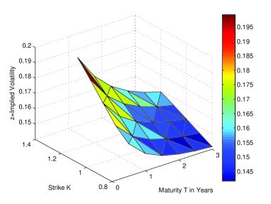
Figure 1: Implied volatility surface for the Heston model

Remark 6.1.

We note that the Heston model is often written in the equivalent form

$$dv =\bar{\kappa}(\eta-v)dt+\sigma\sqrt{v}\,dW_{1}$$

$$dS =rSdt+S\sqrt{v}\,d\mathcal{W}$$

To see the relation of the parameters of this form and the one used in this section, we simply set $v=2X_{1}$, and then get

$$dX_{1} =(\bar{\kappa}\eta-\bar{\kappa}v)dt+\sigma\sqrt{2X_{1}}\,dW_{1}\quad X_{1}(0)=X_{10}$$

$$\frac{dS}{S} =rdt+\sqrt{2X_{1}}\,d\mathcal{W},\quad S(0)=e^{X_{2}(0)}$$

from which we read off

$$k=\bar{\kappa}\eta,\quad\kappa=-\bar{\kappa},\quad X_{10}=v_{0}/2$$

and all other parameters coincide.

7 Affine Transformations and Canonical Representation

As above, we let $X$ be affine on the canonical state space $\mathbb{R}^{m}_{+}\times\mathbb{R}^{n}$ with admissible parameters $a,\alpha_{i},b,\beta_{i}$. Hence, in view of (2.1), for any $x\in\mathbb{R}^{m}_{+}\times\mathbb{R}^{n}$ the process $X=X^{x}$ satisfies

$$dX =(b+{\mathcal{B}}X)\,dt+\rho(X)\,dW$$ (7.1)

$$X(0) =x,$$

and $\rho(x)\rho(x)^{\top}=a+\sum_{i\in I}x_{i}\alpha_{i}$.

It can easily be checked that for every invertible $d\times d$-matrix $\Lambda$, the linear transform

$$Y=\Lambda X$$

satisfies

$$dY=\left(\Lambda b+\Lambda{\mathcal{B}}\Lambda^{-1}Y\right)\,dt+\Lambda\rho\left(\Lambda^{-1}Y\right)\,dW,\quad Y(0)=\Lambda x.$$ (7.2)

Hence, $Y$ has again an affine drift and diffusion matrix

$$\Lambda b+\Lambda{\mathcal{B}}\Lambda^{-1}y\quad\text{and}\quad\Lambda\alpha(\Lambda^{-1}y)\Lambda^{\top},$$ (7.3)

respectively.

On the other hand, the affine short rate model (4.1) can be expressed in terms of $Y(t)$ as

$$r(t)=c+\gamma^{\top}\Lambda^{-1}Y(t)\,.$$ (7.4)

This shows that $Y$ and (7.4) specify an affine short rate model producing the same short rates, and thus bond prices, as $X$ and (4.1). That is, an invertible linear transformation of the state process changes the particular form of the stochastic differential equation (7.1). But it leaves observable quantities, such as short rates and bond prices invariant.

This motivates the question whether there exists a classification method ensuring that affine short rate models with the same observable implications have a unique canonical representation. This topic has been addressed in [10, 9, 24, 8]. We now elaborate on this issue and show that the diffusion matrix $\alpha(x)$ can always be brought into block-diagonal form by a regular linear transform $\Lambda$ with $\Lambda(\mathbb{R}^{m}_{+}\times\mathbb{R}^{n})=\mathbb{R}^{m}_{+}\times\mathbb{R}^{n}$.

We denote by

$${\rm diag}(z_{1},\dots,z_{m})$$

the diagonal matrix with diagonal elements $z_{1},\dots,z_{m}$, and we write $I_{m}$ for the $m\times m$-identity matrix.

Lemma 7.1.

There exists some invertible $d\times d$-matrix $\Lambda$ with $\Lambda(\mathbb{R}^{m}_{+}\times\mathbb{R}^{n})=\mathbb{R}^{m}_{+}\times\mathbb{R}^{n}$ such that $\Lambda\alpha(\Lambda^{-1}y)\Lambda^{\top}$ is block-diagonal of the form

$$\Lambda\alpha(\Lambda^{-1}y)\Lambda^{\top}=\left(\begin{array}[]{cc}{\rm diag}(y_{1},\dots,y_{q},0,\dots,0)&0\\ 0&p+\sum_{i\in I}y_{i}\pi_{i}\end{array}\right)$$

for some integer $0\leq q\leq m$ and symmetric positive semi-definite $n\times n$ matrices $p,\pi_{1},\dots,\pi_{m}$. Moreover, $\Lambda b$ and $\Lambda{\mathcal{B}}\Lambda^{-1}$ meet the respective admissibility conditions (3.1) in lieu of $b$ and ${\mathcal{B}}$.

Proof.

From (2.3) we know that $\Lambda\alpha(x)\Lambda^{\top}$ is block-diagonal for all $x=\Lambda^{-1}y$ if and only if $\Lambda a\Lambda^{\top}$ and $\Lambda\alpha_{i}\Lambda^{\top}$ are block-diagonal for all $i\in I$. By permutation and scaling of the first $m$ coordinate axes (this is a linear bijection from $\mathbb{R}^{m}_{+}\times\mathbb{R}^{n}$ onto itself, which preserves the admissibility of the transformed $b$ and ${\mathcal{B}}$), we may assume that there exists some integer $0\leq q\leq m$ such that $\alpha_{1,11}=\cdots=\alpha_{q,qq}=1$ and $\alpha_{i,ii}=0$ for $q<i\leq m$. Hence $a$ and $\alpha_{i}$ for $q<i\leq m$ are already block-diagonal of the special form

$$a=\left(\begin{array}[]{cc}0&0\\ 0&a_{JJ}\end{array}\right),\quad\alpha_{i}=\left(\begin{array}[]{cc}0&0\\ 0&\alpha_{i,JJ}\end{array}\right).$$

For $1\leq i\leq q$, we may have non-zero off-diagonal elements in the $i$-th row $\alpha_{i,iJ}$. We thus define the $n\times m$-matrix ${D}=(\delta_{1},\dots,\delta_{m})$ with $i$-th column $\delta_{i}=-\alpha_{i,iJ}$ and set

$$\Lambda=\left(\begin{array}[]{cc}I_{m}&0\\ {D}&I_{n}\end{array}\right).$$

One checks by inspection that ${D}$ is invertible and maps $\mathbb{R}^{m}_{+}\times\mathbb{R}^{n}$ onto $\mathbb{R}^{m}_{+}\times\mathbb{R}^{n}$. Moreover,

$${D}\alpha_{i,II}=-\alpha_{i,JI},\quad i\in I.$$

From here we easily verify that

$$\Lambda\alpha_{i}=\left(\begin{array}[]{cc}\alpha_{i,II}&\alpha_{i,IJ}\\ 0&{D}\alpha_{i,IJ}+\alpha_{i,JJ}\end{array}\right),$$

and thus

$$\Lambda\alpha_{i}\Lambda^{\top}=\left(\begin{array}[]{cc}\alpha_{i,II}&0\\ 0&{D}\alpha_{i,IJ}+\alpha_{i,JJ}\end{array}\right).$$

Since $\Lambda a\Lambda^{\top}=a$, the first assertion is proved.

The admissibility conditions for $\Lambda b$ and $\Lambda{\mathcal{B}}\Lambda^{-1}$ can easily be checked as well. ∎

In view of (7.3), (7.4) and Lemma 7.1 we thus obtain the following result.

Theorem 7.2 (Canonical Representation).

Any affine short rate model (4.1), after some modification of $\gamma$ if necessary, admits an $\mathbb{R}^{m}_{+}\times\mathbb{R}^{n}$-valued affine state process $X$ with block-diagonal diffusion matrix of the form

$$\alpha(x)=\left(\begin{array}[]{cc}{\rm diag}(x_{1},\dots,x_{q},0,\dots,0)&0\\ 0&a+\sum_{i\in I}x_{i}\alpha_{i,JJ}\end{array}\right)$$ (7.5)

for some integer $0\leq q\leq m$.

8 Existence and Uniqueness of Affine Processes

All we said about the affine process $X$ so far was under the premise that there exists a unique solution $X=X^{x}$ of the stochastic differential equation (2.1) on some appropriate state space ${\mathcal{X}}\subset\mathbb{R}^{d}$. However, if the diffusion matrix $\rho(x)\rho(x)^{\top}$ is affine then $\rho(x)$ cannot be Lipschitz continuous in $x$ in general. This raises the question whether (2.1) admits a solution at all.

In this section, we show how $X$ can always be realized as unique solution of the stochastic differential equation (2.1), which is (7.1), in the canonical affine framework ${\mathcal{X}}=\mathbb{R}^{m}_{+}\times\mathbb{R}^{n}$ and for particular choices of $\rho(x)$.

We recall from Theorem 2.2 that the affine property of $X$ imposes explicit conditions on $\rho(x)\rho(x)^{\top}$, but not on $\rho(x)$ as such. Indeed, for any orthogonal $d\times d$-matrix $D$, the function $\rho(x)D$ yields the same diffusion matrix, $\rho(x)DD^{\top}\rho(x)^{\top}=\rho(x)\rho(x)^{\top}$, as $\rho(x)$.

On the other hand, from Theorem 3.2 we know that any admissible parameters $a,\alpha_{i},b,\beta_{i}$ in (2.3) uniquely determine the functions $(\phi(\cdot,u),\psi(\cdot,u)):\mathbb{R}_{+}\to\mathbb{C}_{-}\times\mathbb{C}^{m}_{-}\times\mathrm{i}\mathbb{R}^{n}$ as solution of the Riccati equations (3.2), for all $u\in\mathbb{C}^{m}_{-}\times\mathrm{i}\mathbb{R}^{n}$. These in turn uniquely determine the law of the process $X$. Indeed, for any $0\leq t_{1}<t_{2}$ and $u_{1},\,u_{2}\in\mathbb{C}^{m}_{-}\times\mathrm{i}\mathbb{R}^{n}$, we infer by iteration of (2.2)

$${\mathbb{E}}\left[\mathrm{e\;\!}^{u_{1}^{\top}X(t_{1})+u_{2}^{\top}X(t_{2})}\right] ={\mathbb{E}}\left[\mathrm{e\;\!}^{u_{1}^{\top}X(t_{1})}{\mathbb{E}}\left[\mathrm{e\;\!}^{u_{2}^{\top}X(t_{2})}\mid{\mathcal{F}}_{t_{1}}\right]\right]$$

$$={\mathbb{E}}\left[\mathrm{e\;\!}^{u_{1}^{\top}X(t_{1})}\mathrm{e\;\!}^{\phi(t_{2}-t_{1},u_{2})+\psi(t_{2}-t_{1},u_{2})^{\top}X(t_{1})}\right]$$

$$=\mathrm{e\;\!}^{\phi(t_{2}-t_{1},u_{2})+\phi(t_{1},u_{1}+\psi(t_{2}-t_{1},u_{2}))+\psi(t_{1},u_{1}+\psi(t_{2}-t_{1},u_{2}))^{\top}x}.$$

Hence the joint distribution of $(X(t_{1}),X(t_{2}))$ is uniquely determined by the functions $\phi$ and $\psi$. By further iteration of this argument, we conclude that every finite dimensional distribution, and thus the law, of $X$ is uniquely determined by the parameters $a,\alpha_{i},b,\beta_{i}$.

We conclude that the law of an affine process $X$, while uniquely determined by its characteristics (2.3), can be realized by infinitely many variants of the stochastic differential equation (7.1) by replacing $\rho(x)$ by $\rho(x)D$, for any orthogonal $d\times d$-matrix $D$. We now propose a canonical choice of $\rho(x)$ as follows:

• In view of (7.2) and Lemma 7.1, every affine process $X$ on $\mathbb{R}^{m}_{+}\times\mathbb{R}^{n}$ can be written as $X=\Lambda^{-1}Y$ for some invertible $d\times d$-matrix $\Lambda$ and some affine process $Y$ on $\mathbb{R}^{m}_{+}\times\mathbb{R}^{n}$ with block-diagonal diffusion matrix. It is thus enough to consider such $\rho(x)$ where $\rho(x)\rho(x)^{\top}$ is of the form (7.5). Obviously, $\rho(x)\equiv\rho(x_{I})$ is a function of $x_{I}$ only.

• Set $\rho_{IJ}(x)\equiv 0$, $\rho_{JI}(x)\equiv 0$, and

  $$\rho_{II}(x_{I})={\rm diag}(\sqrt{x_{1}},\dots,\sqrt{x_{q}},0,\dots,0).$$

  Chose for $\rho_{JJ}(x_{I})$ any measurable $n\times n$-matrix-valued function satisfying

  $$\rho_{JJ}(x_{I})\rho_{JJ}(x_{I})^{\top}=a+\sum_{i\in I}x_{i}\alpha_{i,JJ}.$$ (8.1)

  In practice, one would determine $\rho_{JJ}(x_{I})$ via Cholesky factorization, see e.g. [31, Theorem 2.2.5]. If $a+\sum_{i\in I}x_{i}\alpha_{i,JJ}$ is strictly positive definite, then $\rho_{JJ}(x_{I})$ turns out to be the unique lower triangular matrix with strictly positive diagonal elements and satisfying (8.1). If $a+\sum_{i\in I}x_{i}\alpha_{i,JJ}$ is merely positive semi-definite, then the algorithm becomes more involved. In any case, $\rho_{JJ}(x_{I})$ will depend measurably on $x_{I}$.

• The stochastic differential equation (7.1) now reads

  $$dX_{I} =(b_{I}+{\mathcal{B}}_{II}X_{I})\,dt+\rho_{II}(X_{I})\,dW_{I}$$ (8.2)

  $$dX_{J} =(b_{J}+{\mathcal{B}}_{JI}X_{I}+{\mathcal{B}}_{JJ}X_{J})\,dt+\rho_{JJ}(X_{I})\,dW_{J}$$

  $$X(0) =x$$

  Lemma 8.2 below asserts the existence and uniqueness of an $\mathbb{R}^{m}_{+}\times\mathbb{R}^{n}$-valued solution $X=X^{x}$, for any $x\in\mathbb{R}^{m}_{+}\times\mathbb{R}^{n}$.

We thus have shown:

Theorem 8.1.

Let $a,\alpha_{i},b,\beta_{i}$ be admissible parameters. Then there exists a measurable function $\rho:\mathbb{R}^{m}_{+}\times\mathbb{R}^{n}\to\mathbb{R}^{d\times d}$ with $\rho(x)\rho(x)^{\top}=a+\sum_{i\in I}x_{i}\alpha_{i}$, and such that, for any $x\in\mathbb{R}^{m}_{+}\times\mathbb{R}^{n}$, there exists a unique $\mathbb{R}^{m}_{+}\times\mathbb{R}^{n}$-valued solution $X=X^{x}$ of (7.1).

Moreover, the law of $X$ is uniquely determined by $a,\alpha_{i},b,\beta_{i}$, and does not depend on the particular choice of $\rho$.

The proof of the following lemma uses the concept of a weak solution. The interested reader will find detailed background in e.g. [25, Section 5.3].

Lemma 8.2.

For any $x\in\mathbb{R}^{m}_{+}\times\mathbb{R}^{n}$, there exists a unique $\mathbb{R}^{m}_{+}\times\mathbb{R}^{n}$-valued solution $X=X^{x}$ of (8.2).

Proof.

First, we extend $\rho$ continuously to $\mathbb{R}^{d}$ by setting $\rho(x)=\rho(x_{1}^{+},\dots,x_{m}^{+})$, where we denote $x_{i}^{+}=\max(0,x_{i})$.

Now observe that $X_{I}$ solves the autonomous equation

$$dX_{I}=(b_{I}+{\mathcal{B}}_{II}X_{I})\,dt+\rho_{II}(X_{I})\,dW_{I},\quad X_{I}(0)=x_{I}.$$ (8.3)

Obviously, there exists a finite constant $K$ such that the linear growth condition

$$\|b_{I}+{\mathcal{B}}_{II}x_{I}\|^{2}+\|\rho(x_{I})\|^{2}\leq K(1+\|x_{I}\|^{2})$$

is satisfied for all $x\in\mathbb{R}^{m}$. By [22, Theorems 2.3 and 2.4] there exists a weak solution of (8.3). On the other hand, (8.3) is exactly of the form as assumed in [35, Theorem 1], which implies that pathwise uniqueness holds for (8.3). The Yamada–Watanabe Theorem, see [35, Corollary 3] or [25, Corollary 5.3.23], thus implies that there exists a unique solution $X_{I}=X_{I}^{x_{I}}$ of (8.3), for all $x_{I}\in\mathbb{R}^{m}$.

Given $X_{I}^{x_{I}}$, it is then easily seen that

$$X_{J}(t) =\mathrm{e\;\!}^{{\mathcal{B}}_{JJ}t}\left(x_{J}+\int_{0}^{t}\mathrm{e\;\!}^{-{\mathcal{B}}_{JJ}s}(b_{J}+{\mathcal{B}}_{JI}X_{I}(s))\,ds\right.$$

$$+\left.\int_{0}^{t}\mathrm{e\;\!}^{-{\mathcal{B}}_{JJ}s}\rho_{JJ}(X_{I}(s))\,dW_{J}(s)\right)$$

is the unique solution to the second equation in (8.2).

Admissibility of the parameters $b$ and $\beta_{i}$ and the stochastic invariance Lemma B.1 eventually imply that $X_{I}=X_{I}^{x_{I}}$ is $\mathbb{R}^{m}_{+}$-valued for all $x_{I}\in\mathbb{R}^{m}_{+}$. Whence the lemma is proved. ∎

Appendix A On the Regularity of Characteristic Functions

This auxiliary section provides some analytic regularity results for characteristic functions, which are of independent interest. These results enter the main text only via the proof of Theorem 3.3. This section may thus be skipped at the first reading.

Let $\nu$ be a bounded measure on $\mathbb{R}^{d}$, and denote by

$$G(z)=\int_{\mathbb{R}^{d}}\mathrm{e\;\!}^{z^{\top}x}\,\nu(dx)$$

its characteristic function for $z\in\mathrm{i}\mathbb{R}^{d}$. Note that $G(z)$ is actually well defined for $z\in{\mathcal{S}}(V)$ where

$$V=\left\{y\in\mathbb{R}^{d}\mid\int_{\mathbb{R}^{d}}\mathrm{e\;\!}^{y^{\top}x}\,\nu(dx)<\infty\right\}.$$

We first investigate the interplay between the (marginal) moments of $\nu$ and the corresponding (partial) regularity of $G$.

Lemma A.1.

Denote $g(y)=G(iy)$ for $y\in\mathbb{R}^{d}$, and let $k\in\mathbb{N}$ and $1\leq i\leq d$.

If $\partial_{y_{i}}^{2k}g(0)$ exists then

$$\int_{\mathbb{R}^{d}}|x_{i}|^{2k}\,\nu(dx)<\infty.$$

On the other hand, if $\int_{\mathbb{R}^{d}}\|x\|^{k}\,\nu(dx)<\infty$ then $g\in C^{k}$ and

$$\partial_{y_{i_{1}}}\cdots\partial_{y_{i_{l}}}g(y)=\mathrm{i}^{l}\int_{\mathbb{R}^{d}}x_{i_{1}}\cdots x_{i_{l}}\,\mathrm{e\;\!}^{\mathrm{i}y^{\top}x}\,\nu(dx)$$

for all $y\in\mathbb{R}^{d}$, $1\leq i_{1},\dots,i_{l}\leq d$ and $1\leq l\leq k$.

Proof.

As usual, let $e_{i}$ denote the $i$th standard basis vector in $\mathbb{R}^{d}$. Observe that $s\mapsto g(se_{i})$ is the characteristic function of the image measure of $\nu$ on $\mathbb{R}$ by the mapping $x\mapsto x_{i}$. Since $\partial_{s}^{2k}g(se_{i})|_{s=0}=\partial_{y_{i}}^{2k}g(0)$, the assertion follows from the one-dimensional case, see [30, Theorem 2.3.1].

The second part of the lemma follows by differentiating under the integral sign, which is allowed by dominated convergence. ∎

Lemma A.2.

The set $V$ is convex. Moreover, if $U\subset V$ is an open set in $\mathbb{R}^{d}$, then $G$ is analytic on the open strip ${\mathcal{S}}(U)$ in $\mathbb{C}^{d}$.

Proof.

Since $G:\mathbb{R}^{d}\to[0,\infty]$ is a convex function, its domain $V=\{y\in\mathbb{R}^{d}\mid G(y)<\infty\}$ is convex, and so is every level set $V_{l}=\{y\in\mathbb{R}^{d}\mid G(y)\leq l\}$ for $l\geq 0$.

Now let $U\subset V$ be an open set in $\mathbb{R}^{d}$. Since any convex function on $\mathbb{R}^{d}$ is continuous on the open interior of its domain, see [32, Theorem 10.1], we infer that $G$ is continuous on $U$. We may thus assume that $U_{l}=\{y\in\mathbb{R}^{d}\mid G(y)<l\}\cap U\subset V_{l}$ is open in $\mathbb{R}^{d}$ and non-empty for $l>0$ large enough.

Let $z\in{\mathcal{S}}(U_{l})$ and $(z_{n})$ be a sequence in ${\mathcal{S}}(U_{l})$ with $z_{n}\to z$. For $n$ large enough, there exists some $p>1$ such that $pz_{n}\in{\mathcal{S}}(U_{l})$. This implies $p\mathbb{R}ez_{n}\in V_{l}$ and hence

$$\int_{\mathbb{R}^{d}}\left|\mathrm{e\;\!}^{z_{n}^{\top}x}\right|^{p}\,\nu(dx)\leq l.$$

Hence the class of functions $\{\mathrm{e\;\!}^{z_{n}^{\top}x}\mid n\in\mathbb{N}\}$ is uniformly integrable with respect to $\nu$, see [34, 13.3]. Since $\mathrm{e\;\!}^{z_{n}^{\top}x}\to\mathrm{e\;\!}^{z^{\top}x}$ for all $x$, we conclude by Lebesgue’s convergence theorem that

$$|G(z_{n})-G(z)|\leq\int_{\mathbb{R}^{d}}\left|\mathrm{e\;\!}^{z_{n}^{\top}x}-\mathrm{e\;\!}^{z^{\top}x}\right|\,\nu(dx)\to 0.$$

Hence $G$ is continuous on ${\mathcal{S}}(U_{l})$.

It thus follows from the Cauchy formula, see [11, Section IX.9], that $G$ is analytic on ${\mathcal{S}}(U_{l})$ if and only if, for every $z\in{\mathcal{S}}(U_{l})$ and $1\leq i\leq d$, the function $\zeta\mapsto G(z+\zeta e_{i})$ is analytic on $\{\zeta\in\mathbb{C}\mid z+\zeta e_{i}\in{\mathcal{S}}(U_{l})\}$. Here, as usual, we denote $e_{i}$ the $i$th standard basis vector in $\mathbb{R}^{d}$.

We thus let $z\in{\mathcal{S}}(U_{l})$ and $1\leq i\leq d$. Then there exists some $\epsilon_{-}<0<\epsilon_{+}$ such that $z+\zeta e_{i}\in{\mathcal{S}}(U_{l})$ for all $\zeta\in{\mathcal{S}}([\epsilon_{-},\epsilon_{+}])$. In particular, $|\mathrm{e\;\!}^{(z+\epsilon_{-}e_{i})^{\top}x}|\,\nu(dx)$ and $|\mathrm{e\;\!}^{(z+\epsilon_{+}e_{i})^{\top}x}|\,\nu(dx)$ are bounded measures on $\mathbb{R}^{d}$. By dominated convergence, it follows that the two summands

$$G(z+\zeta e_{i}) =\int_{\{x_{i}<0\}}\mathrm{e\;\!}^{(\zeta-\epsilon_{-})x_{i}}\,\mathrm{e\;\!}^{(z+\epsilon_{-}e_{i})^{\top}x}\,\nu(dx)$$

$$+\int_{\{x_{i}\geq 0\}}\mathrm{e\;\!}^{(\zeta-\epsilon_{+})x_{i}}\,\mathrm{e\;\!}^{(z+\epsilon_{+}e_{i})^{\top}x}\,\nu(dx),$$

are complex differentiable, and thus $G$ is analytic, in $\zeta\in{\mathcal{S}}((\epsilon_{-},\epsilon_{+}))$. Whence $G$ is analytic on ${\mathcal{S}}(U_{l})$. Since ${\mathcal{S}}(U)=\cup_{l>0}{\mathcal{S}}(U_{l})$, the lemma follows. ∎

In general, $V$ does not have an open interior in $\mathbb{R}^{d}$. The next lemma provides sufficient conditions for the existence of an open set $U\subset V$ in $\mathbb{R}^{d}$.

Lemma A.3.

Let $U^{\prime}$ be an open neighborhood of $0$ in $\mathbb{C}^{d}$ and $h$ an analytic function on $U^{\prime}$. Suppose that $U=U^{\prime}\cap\mathbb{R}^{d}$ is star-shaped around $0$ and $G(z)=h(z)$ for all $z\in U^{\prime}\cap\mathrm{i}\mathbb{R}^{d}$. Then $U\subset V$ and $G=h$ on $U^{\prime}\cap{\mathcal{S}}(U)$.

Proof.

We first suppose that $U^{\prime}=P_{\rho}$ for the open polydisc

$$P_{\rho}=\left\{z\in\mathbb{C}^{d}\mid|z_{i}|<\rho_{i},\;1\leq i\leq d\right\},$$

for some $\rho=(\rho_{1},\dots,\rho_{d})\in\mathbb{R}^{d}_{++}$. Note the symmetry $\mathrm{i}P_{\rho}=P_{\rho}$.

As in Lemma A.1, we denote $g(y)=G(iy)$ for $y\in\mathbb{R}^{d}$. By assumption, $g(y)=h(\mathrm{i}y)$ for all $y\in P_{\rho}\cap\mathbb{R}^{d}$. Hence $g$ is analytic on $P_{\rho}\cap\mathbb{R}^{d}$, and the Cauchy formula, [11, Section IX.9], yields

$$g(y)=\sum_{i_{1},\dots,i_{d}\in\mathbb{N}_{0}}c_{i_{1},\dots,i_{d}}y_{1}^{i_{1}}\cdots y_{d}^{i_{d}}\quad\text{for $y\in P_{\rho}\cap\mathbb{R}^{d}$}$$

where $\sum_{i_{1},\dots,i_{d}\in\mathbb{N}_{0}}c_{i_{1},\dots,i_{d}}z_{1}^{i_{1}}\cdots z_{d}^{i_{d}}=h(\mathrm{i}z)$ for all $z\in P_{\rho}$. This power series is absolutely convergent on $P_{\rho}$, that is,

$$\sum_{i_{1},\dots,i_{d}\in\mathbb{N}_{0}}|c_{i_{1},\dots,i_{d}}|\,|z_{1}^{i_{1}}\cdots z_{d}^{i_{d}}|<\infty\quad\text{for all $z\in P_{\rho}$.}$$

From the first part of Lemma A.1, we infer that $\nu$ possesses all moments, that is, $\int_{\mathbb{R}^{d}}\|x\|^{k}\,\nu(dx)<\infty$ for all $k\in\mathbb{N}$. From the second part of Lemma A.1 thus

$$c_{i_{1},\dots,i_{d}}=\frac{\mathrm{i}^{i_{1}+\cdots+i_{d}}}{i_{1}!\cdots i_{d}!}\int_{\mathbb{R}^{d}}x_{1}^{i_{1}}\cdots x_{d}^{i_{d}}\,\nu(dx).$$

From the inequality $|x_{i}|^{2k-1}\leq(x_{i}^{2k}+x^{2k-2}_{i})/2$, for $k\in\mathbb{N}$, and the above properties, we infer that for all $z\in P_{\rho}$,

$$\int_{\mathbb{R}^{d}}\mathrm{e\;\!}^{\sum_{i=1}^{d}|z_{i}|\,|x_{i}|}\,\nu(dx)=\sum_{i_{1},\dots,i_{d}\in\mathbb{N}_{0}}\frac{|z_{1}^{i_{1}}\cdots z_{d}^{i_{d}}|}{i_{1}!\cdots i_{d}!}\int_{\mathbb{R}^{d}}|x_{1}^{i_{1}}\cdots x_{d}^{i_{d}}|\,\nu(dx)<\infty$$

Hence $P_{\rho}\cap\mathbb{R}^{d}\subset V$, and Lemma A.2 implies that $G$ is analytic on ${\mathcal{S}}(P_{\rho}\cap\mathbb{R}^{d})$. Since the power series for $G$ and $h$ coincide on $P_{\rho}\cap\mathrm{i}\mathbb{R}^{d}$, we conclude that $G=h$ on $P_{\rho}$, and the lemma is proved for $U^{\prime}=P_{\rho}$.

Now let $U^{\prime}$ be an open neighborhood of $0$ in $\mathbb{C}^{d}$. Then there exists some open polydisc $P_{\rho}\subset U^{\prime}$ with $\rho\in\mathbb{R}^{d}_{++}$. By the preceding case, we have $P_{\rho}\cap\mathbb{R}^{d}\subset V$ and $G=h$ on $P_{\rho}$. In view of Lemma A.2 it thus remains to show that $U=U^{\prime}\cap\mathbb{R}^{d}\subset V$.

To this end, let $a\in U$. Since $U$ is star-shaped around $0$ in ${\mathbb{R}}^{d}$, there exists some $s_{1}>1$ such that $sa\in U$ for all $s\in[0,s_{1}]$ and $h(sa)$ is analytic in $s\in(0,s_{1})$. On the other hand, there exists some $0<s_{0}<s_{1}$ such that $sa\in P_{\rho}\cap{\mathbb{R}}^{d}$ for all $s\in[0,s_{0}]$, and $G(sa)=h(sa)$ for $s\in(0,s_{0})$. This implies

$$\int_{\{a^{\top}x\geq 0\}}\mathrm{e\;\!}^{sa^{\top}x}\,\nu(dx)=h(sa)-\int_{\{a^{\top}x<0\}}\mathrm{e\;\!}^{sa^{\top}x}\,\nu(dx)$$

for $s\in(0,s_{0})$. By Lemma A.2, the right hand side is an analytic function in $s\in(0,s_{1})$. We conclude by Lemma A.4 below, for $\mu$ defined as the image measure of $\nu$ on ${\mathbb{R}}_{+}$ by the mapping $x\mapsto a^{\top}x$, that $a\in V$. Hence the lemma is proved. ∎

Lemma A.4.

Let $\mu$ be a bounded measure on ${\mathbb{R}}_{+}$, and $h$ an analytic function on $(0,s_{1})$, such that

$$\int_{{\mathbb{R}}_{+}}\mathrm{e\;\!}^{sx}\,\mu(dx)=h(s)$$ (A.1)

for all $s\in(0,s_{0})$, for some numbers $0<s_{0}<s_{1}$. Then (A.1) also holds for $s\in(0,s_{1})$.

Proof.

Denote $f(s)=\int_{{\mathbb{R}}_{+}}\mathrm{e\;\!}^{sx}\,\mu(dx)$ and define $s_{\infty}=\sup\left\{s>0\mid f(s)<\infty\right\}\geq s_{0}$, such that

$$f(s)=+\infty\quad\text{for $s\geq s_{\infty}$.}$$ (A.2)

We assume, by contradiction, that $s_{\infty}<s_{1}$. Then there exists some $s_{\ast}\in(0,s_{\infty})$ and $\epsilon>0$ such that $s_{\ast}<s_{\infty}<s_{\ast}+\epsilon$ and such that $h$ can be developed in an absolutely convergent power series

$$h(s)=\sum_{k\geq 0}\frac{c_{k}}{k!}(s-s_{\ast})^{k}\quad\text{for $s\in(s_{\ast}-\epsilon,s_{\ast}+\epsilon)$.}$$

In view of Lemma A.2, $f$ is analytic, and thus $f=h$, on $(0,s_{\infty})$. Hence we obtain, by dominated convergence,

$$c_{k}=\frac{d^{k}}{ds^{k}}h(s)|_{s=s_{\ast}}=\frac{d^{k}}{ds^{k}}f(s)|_{s=s_{\ast}}=\int_{{\mathbb{R}}_{+}}x^{k}\mathrm{e\;\!}^{s_{\ast}x}\,\mu(dx)\geq 0.$$

By monotone convergence, we conclude

$$h(s)=\sum_{k\geq 0}\int_{{\mathbb{R}}_{+}}\frac{x^{k}}{k!}(s-s_{\ast})^{k}\mathrm{e\;\!}^{s_{\ast}x}\,\mu(dx)=\int_{{\mathbb{R}}_{+}}\sum_{k\geq 0}\frac{x^{k}}{k!}(s-s_{\ast})^{k}\mathrm{e\;\!}^{s_{\ast}x}\,\mu(dx)=\int_{{\mathbb{R}}_{+}}\mathrm{e\;\!}^{sx}\,\mu(dx)$$

for all $s\in(s_{\ast},s_{\ast}+\epsilon)$. But this contradicts (A.2). Whence $s_{\infty}\geq s_{1}$, and the lemma is proved. ∎

Appendix B Invariance and Comparison Results for Differential Equations

In this section we deliver invariance and comparison results for stochastic and ordinary differential equations, which are used in the proofs of the main Theorems 3.2, 3.3 and 4.1 and Lemma 8.2 above.

We start with an invariance result for the stochastic differential equation (2.1).

Lemma B.1.

Suppose $b$ and $\rho$ in (2.1) admit a continuous and measurable extension to $\mathbb{R}^{d}$, respectively, and such that $a$ is continuous on $\mathbb{R}^{d}$. Let $u\in\mathbb{R}^{d}\setminus\{0\}$ and define the half space

$$H=\{x\in\mathbb{R}^{d}\mid u^{\top}x\geq 0\},$$

its interior $H^{0}=\{x\in\mathbb{R}^{d}\mid u^{\top}x>0\}$, and its boundary $\partial H=\{x\in H\mid u^{\top}x=0\}$.

1. Fix $x\in\partial H$ and let $X=X^{x}$ be a solution of (2.1). If $X(t)\in H$ for all $t\geq 0$, then necessarily

   $$u^{\top}a(x)\,u =0$$ (B.1)

   $$u^{\top}b(x) \geq 0.$$ (B.2)

2. Conversely, if (B.1) and (B.2) hold for all $x\in\mathbb{R}^{d}\setminus H^{0}$, then any solution $X$ of (2.1) with $X(0)\in H$ satisfies $X(t)\in H$ for all $t\geq 0$.

Intuitively speaking, (B.1) means that the diffusion must be “parallel to the boundary”, and (B.2) says that the drift must be “inward pointing” at the boundary of $H$.

Proof.

Fix $x\in\partial H$ and let $X=X^{x}$ be a solution of (2.1). Hence

$$u^{\top}X(t)=\int_{0}^{t}u^{\top}b(X(s))\,ds+\int_{0}^{t}u^{\top}\rho(X(s))\,dW(s).$$

Since $a$ and $b$ are continuous, there exists a stopping time $\tau_{1}>0$ and a finite constant $K$ such that

$$|u^{\top}b(X(t\wedge\tau_{1}))|\leq K$$

and

$$\|u^{\top}\rho(X(t\wedge\tau_{1}))\|^{2}=u^{\top}a(X(t\wedge\tau_{1}))\,u\leq K$$

for all $t\geq 0$. In particular, the stochastic integral part of $u^{\top}X(t\wedge\tau_{1})$ is a martingale. Hence

$${\mathbb{E}}\left[u^{\top}X(t\wedge\tau_{1})\right]={\mathbb{E}}\left[\int_{0}^{t\wedge\tau_{1}}u^{\top}b(X(s))\,ds\right],\quad t\geq 0.$$

We now argue by contradiction, and assume first that $u^{\top}b(x)<0$. By continuity of $b$ and $X(t)$, there exists some $\epsilon>0$ and a stopping time $\tau_{2}>0$ such that $u^{\top}b(X(t))\leq-\epsilon$ for all $t\leq\tau_{2}$. In view of the above this implies

$${\mathbb{E}}\left[u^{\top}X(\tau_{2}\wedge\tau_{1})\right]<0.$$

This contradicts $X(t)\in H$ for all $t\geq 0$, whence (B.2) holds.

As for (B.1), let $C>0$ be a finite constant and define the stochastic exponential $Z_{t}={\mathcal{E}}(-C\int_{0}^{t}u^{\top}\rho(X)\,dW)$. Then $Z$ is a strictly positive local martingale. Integration by parts yields

$$u^{\top}X(t)Z(t)=\int_{0}^{t}Z(s)\left(u^{\top}b(X(s))-C\,u^{\top}a(X(s))\,u\right)ds+M(t)$$

where $M$ is a local martingale. Hence there exists a stopping time $\tau_{3}>0$ such that for all $t\geq 0$,

$${\mathbb{E}}\left[u^{\top}X(t\wedge\tau_{3})Z(t\wedge\tau_{3})\right]={\mathbb{E}}\left[\int_{0}^{t\wedge\tau_{3}}Z(s)\left(u^{\top}b(X(s))-C\,u^{\top}a(X(s))\,u\right)ds\right].$$

Now assume that $u^{\top}a(x)\,u0$. By continuity of $a$ and $X(t)$, there exists some $\epsilon>0$ and a stopping time $\tau_{4}>0$ such that $u^{\top}a(X(t))\,u\geq\epsilon$ for all $t\leq\tau_{4}$. For $C>K/\epsilon$, this implies

$${\mathbb{E}}\left[u^{\top}X(\tau_{4}\wedge\tau_{3}\wedge\tau_{1})Z(\tau_{4}\wedge\tau_{3}\wedge\tau_{1})\right]<0.$$

This contradicts $X(t)\in H$ for all $t\geq 0$. Hence (B.1) holds, and part (i) is proved.

As for part (ii), suppose (B.1) and (B.2) hold for all $x\in\mathbb{R}^{d}\setminus H^{0}$, and let $X$ be a solution of (2.1) with $X(0)\in H$. For $\delta,\epsilon>0$ define the stopping time

$$\tau_{\delta,\epsilon}=\inf\left\{t\mid\text{$u^{\top}X(t)\leq-\epsilon$ and $u^{\top}X(s)<0$ for all $s\in[t-\delta,t]$}\right\}.$$

Then on $\{\tau_{\delta,\epsilon}<\infty\}$ we have $u^{\top}\rho(X(s))=0$ for $\tau_{\delta,\epsilon}-\delta\leq s\leq\tau_{\delta,\epsilon}$ and thus

$$0>u^{\top}X(\tau_{\delta,\epsilon})-u^{\top}X(\tau_{\delta,\epsilon}-\delta)=\int_{\tau_{\delta,\epsilon}-\delta}^{\tau_{\delta,\epsilon}}u^{\top}b(X(s))\,ds\geq 0,$$

a contradiction. Hence $\tau_{\delta,\epsilon}=\infty$. Since $\delta,\epsilon>0$ were arbitrary, we conclude that $u^{\top}X(t)\geq 0$ for all $t\geq 0$, as desired. Whence the lemma is proved. ∎

It is straightforward to extend Lemma B.1 towards a polyhedral convex set $\cap_{i=1}^{k}H_{i}$ with half-spaces $H_{i}=\{x\in\mathbb{R}^{d}\mid u_{i}^{\top}x\geq 0\}$, for some elements $u_{1},\dots,u_{k}\in\mathbb{R}^{d}\setminus\{0\}$ and some $k\in\mathbb{N}$. This holds in particular for the canonical state space $\mathbb{R}^{m}_{+}\times\mathbb{R}^{n}$. Moreover, Lemma B.1 includes time-inhomogeneous ordinary differential equations as special case. The proofs of the following two corollaries are left to the reader.

Corollary B.2.

Let $H_{i}=\{x\in\mathbb{R}^{d}\mid x_{i}\geq 0\}$ denote the $i$-th canonical half space in ${\mathbb{R}}^{d}$, for $i=1,\dots,m$. Let $b:{\mathbb{R}}_{+}\times{\mathbb{R}}^{d}\to{\mathbb{R}}^{d}$ be a continuous map satisfying, for all $t\geq 0$,

$$b(t,x) =b(t,x_{1}^{+},\dots,x_{m}^{+},x_{m+1},\dots,x_{d})\quad\text{for all $x\in{\mathbb{R}}^{d}$, and}$$

$$b_{i}(t,x) \geq 0\quad\text{for all $x\in\partial H_{i}$, $i=1,\dots,m$.}$$

Then any solution $f$ of

$$\partial_{t}f(t)=b(t,f(t))$$

with $f(0)\in{\mathbb{R}}^{m}_{+}\times{\mathbb{R}}^{n}$ satisfies $f(t)\in{\mathbb{R}}^{m}_{+}\times{\mathbb{R}}^{n}$ for all $t\geq 0$.

Corollary B.3.

Let $B(t)$ and $C(t)$ be continuous ${\mathbb{R}}^{m\times m}$- and ${\mathbb{R}}^{m}_{+}$-valued parameters, respectively, such that $B_{ij}(t)\geq 0$ whenever $i\neq j$. Then the solution $f$ of the linear differential equation in ${\mathbb{R}}^{m}$

$$\partial_{t}f(t)=B(t)\,f(t)+C(t)$$

with $f(0)\in\mathbb{R}^{m}_{+}$ satisfies $f(t)\in{\mathbb{R}}^{m}_{+}$ for all $t\geq 0$.

Here and subsequently, we let $\succeq$ denote the partial order on ${\mathbb{R}}^{m}$ induced by the cone ${\mathbb{R}}^{m}_{+}$. That is, $x\succeq y$ if $x-y\in{\mathbb{R}}^{m}_{+}$. Then Corollary B.3 may be rephrased, for $C(t)\equiv 0$, by saying that the operator $\mathrm{e\;\!}^{\int_{0}^{t}B(s)\,ds}$ is $\succeq$-order preserving, i.e. $\mathrm{e\;\!}^{\int_{0}^{t}B(s)\,ds}{\mathbb{R}}^{m}_{+}\subseteq{\mathbb{R}}^{m}_{+}$.

Next, we consider time-inhomogeneous Riccati equations in ${\mathbb{R}}^{m}$ of the special form

$$\partial_{t}f_{i}(t)=A_{i}f_{i}(t)^{2}+B_{i}^{\top}f(t)+C_{i}(t),\quad i=1,\dots,m,$$ (B.3)

for some parameters $A,B,C(t)$ satisfying the following admissibility conditions

$$\begin{gathered}A=(A_{1},\dots,A_{m})\in{\mathbb{R}}^{m},\\ B_{i,j}\geq 0\quad\text{for $1\leq i\neq j\leq m$,}\\ \text{$C(t)=(C_{1}(t),\dots,C_{m}(t))$ continuous ${\mathbb{R}}^{m}$-valued.}\end{gathered}$$ (B.4)

The following lemma provides a comparison result for (B.3). It shows, in particular, that the solution of (B.3) is uniformly bounded from below on compacts with respect to $\succeq$ if $A\succeq 0$.

Lemma B.4.

Let $A^{(k)},B,C^{(k)}$, $k=1,2$, be parameters satisfying the admissibility conditions (B.4), and

$$A^{(1)}\preceq A^{(2)},\quad C^{(1)}(t)\preceq C^{(2)}(t).$$ (B.5)

Let $\tau>0$ and $f^{(k)}:[0,\tau)\to{\mathbb{R}}^{m}$ be solutions of (B.4) with $A$ and $C$ replaced by $A^{(k)}$ and $C^{(k)}$, respectively, $k=1,2$. If $f^{(1)}(0)\preceq f^{(2)}(0)$ then $f^{(1)}(t)\preceq f^{(2)}(t)$ for all $t\in[0,\tau)$. If, moreover, $A^{(1)}=0$ then

$$\mathrm{e\;\!}^{Bt}\left(f^{(1)}(0)+\int_{0}^{t}\mathrm{e\;\!}^{-Bs}C^{(1)}(s)\,ds\right)\preceq f^{(2)}(t)$$

for all $t\in[0,\tau)$.

Proof.

The function $f=f^{(2)}-f^{(1)}$ solves

$$\partial_{t}f_{i}(t) =A_{i}^{(2)}\left(f_{i}^{(2)}(t)\right)^{2}-A_{i}^{(1)}\left(f_{i}^{(1)}(t)\right)^{2}+B_{i}^{\top}f+C^{(2)}_{i}(t)-C^{(1)}_{i}(t)$$

$$=\left(A_{i}^{(2)}-A_{i}^{(1)}\right)\left(f_{i}^{(2)}(t)\right)^{2}+A_{i}^{(1)}\left(f_{i}^{(2)}(t)+f_{i}^{(1)}(t)\right)f_{i}(t)+B_{i}^{\top}f(t)+C^{(2)}_{i}(t)-C^{(1)}_{i}(t)$$

$$=\widetilde{B_{i}}(t)^{\top}f(t)+\widetilde{C_{i}}(t),$$

where we write

$$\widetilde{B_{i}}(t) =B_{i}+A_{i}^{(1)}\left(f_{i}^{(2)}(t)+f_{i}^{(1)}(t)\right)e_{i},$$

$$\widetilde{C_{i}}(t) =\left(A_{i}^{(2)}-A_{i}^{(1)}\right)\left(f_{i}^{(2)}(t)\right)^{2}+C^{(2)}_{i}(t)-C^{(1)}_{i}(t).$$

Note that $\widetilde{B}=(\widetilde{B}_{i,j})$ and $\widetilde{C}$ satisfy the assumptions of Corollary B.3 in lieu of $B$ and $C$, and $f(0)\in{\mathbb{R}}^{m}_{+}$. Hence Corollary B.3 implies $f(t)\in{\mathbb{R}}^{m}_{+}$ for all $t\in[0,\tau)$, as desired. The last statement of the lemma follows by the variation of constants formula for $f^{(1)}(t)$. ∎

After these preliminary comparison results for the Riccati equation (B.3), we now can state and prove an important result for the system of Riccati equations (3.2). The following is an essential ingredient of the proof of Theorem 3.3. It is inspired by the line of arguments in Glasserman and Kim [16].

Lemma B.5.

Let ${\mathcal{D}}_{\mathbb{R}}$ denote the maximal domain for the system of Riccati equations (3.2). Let $(\tau,u)\in{\mathcal{D}}_{\mathbb{R}}$. Then

1. ${\mathcal{D}}_{\mathbb{R}}(\tau)$ is star-shaped around zero.

2. $\theta^{\ast}=\sup\{\theta\geq 0\mid\theta u\in{\mathcal{D}}_{\mathbb{R}}(\tau)\}$ satisfies either $\theta^{\ast}=\infty$ or $\lim_{\theta\uparrow\theta^{\ast}}\|\psi_{I}(t,\theta u)\|=\infty$. In the latter case, there exists some $x^{\ast}\in{\mathbb{R}}^{m}_{+}\times{\mathbb{R}}^{n}$ such that $\lim_{\theta\uparrow\theta^{\ast}}\phi(\tau,\theta u)+\psi(\tau,\theta u)^{\top}x^{\ast}=\infty$.

Proof.

We first assume that the matrices $\alpha_{i}$ are block-diagonal, such that $\alpha_{i,iJ}=0$, for all $i=1,\dots,m$.

Fix $\theta\in(0,1]$. We claim that $\theta u\in{\mathcal{D}}_{\mathbb{R}}(\tau)$. It follows by inspection that $f^{(\theta)}(t)=\frac{\psi_{I}(t,\theta u)}{\theta}$ solves (B.3) with

$$A_{i}^{(\theta)}=\frac{1}{2}\theta\alpha_{i,ii},\quad B={\mathcal{B}}_{II}^{\top},\quad C^{(\theta)}_{i}(t)=\beta_{i,J}^{\top}\psi_{J}(t,u)+\frac{1}{2}\psi_{J}(t,u)^{\top}\theta\alpha_{i,JJ}\psi_{J}(t,u),$$

and $f(0)=u$. Lemma B.4 thus implies that $f^{(\theta)}(t)$ is nice behaved, as

$$\mathrm{e\;\!}^{{\mathcal{B}}_{II}^{\top}t}\left(u+\int_{0}^{t}\mathrm{e\;\!}^{-{\mathcal{B}}_{II}^{\top}s}C^{(0)}(s)\,ds\right)\preceq f^{(\theta)}(t)\preceq\psi_{I}(t,u),$$ (B.6)

for all $t\in[0,t_{+}(\theta u))\cap[0,\tau]$. By the maximality of ${\mathcal{D}}_{\mathbb{R}}$ we conclude that $\tau<t_{+}(\theta u)$, which implies $\theta u\in{\mathcal{D}}_{\mathbb{R}}(\tau)$, as desired. Hence ${\mathcal{D}}_{\mathbb{R}}(\tau)$ is star-shaped around zero, which is part (i).

Next suppose that $\theta^{\ast}<\infty$. Since ${\mathcal{D}}_{\mathbb{R}}(\tau)$ is open, this implies $\theta^{\ast}u\notin{\mathcal{D}}_{\mathbb{R}}(\tau)$ and thus $t_{+}(\theta^{\ast}u)\leq\tau$. From part (i) we know that $(t,\theta u)\in{\mathcal{D}}_{\mathbb{R}}$ for all $t<t_{+}(\theta^{\ast}u)$ and $0\leq\theta\leq\theta^{\ast}$. On the other hand, there exists a sequence $t_{n}\uparrow t_{+}(\theta^{\ast}u)$ such that $\|\psi_{I}(t_{n},\theta^{\ast}u)\|>n$ for all $n\in{\mathbb{N}}$. By continuity of $\psi$ on ${\mathcal{D}}_{\mathbb{R}}$, we conclude that there exists some sequence $\theta_{n}\uparrow\theta^{\ast}$ with $\|\psi_{I}(t_{n},\theta_{n}u)-\psi_{I}(t_{n},\theta^{\ast}u)\|\leq 1/n$ and hence

$$\lim_{n}\|\psi_{I}(t_{n},\theta_{n}u)\|=\infty.$$ (B.7)

Applying Lemma B.4 as above, where initial time $t=0$ is shifted to $t_{n}$, yields

$$g_{n}:=\mathrm{e\;\!}^{{\mathcal{B}}_{II}^{\top}(\tau-t_{n})}\left(f^{(\theta_{n})}(t_{n})+\int_{t_{n}}^{\tau}\mathrm{e\;\!}^{{\mathcal{B}}_{II}^{\top}(t_{n}-s)}C^{(0)}(s)\,ds\right)\preceq f^{(\theta_{n})}(\tau).$$

Corollary B.3 implies that $\mathrm{e\;\!}^{{\mathcal{B}}_{II}^{\top}(\tau-t_{n})}$ is $\succeq$-order preserving. That is, $\mathrm{e\;\!}^{{\mathcal{B}}_{II}^{\top}(\tau-t_{n})}{\mathbb{R}}^{m}_{+}\subseteq{\mathbb{R}}^{m}_{+}$. Hence, in view of (B.6) for $f^{(\theta_{n})}(t_{n})$,

$$g_{n} \succeq\mathrm{e\;\!}^{{\mathcal{B}}_{II}^{\top}(\tau-t_{n})}\left(\mathrm{e\;\!}^{{\mathcal{B}}_{II}^{\top}t_{n}}\left(u+\int_{0}^{t_{n}}\mathrm{e\;\!}^{-{\mathcal{B}}_{II}^{\top}s}C^{(0)}(s)\,ds\right)+\int_{t_{n}}^{\tau}\mathrm{e\;\!}^{{\mathcal{B}}_{II}^{\top}(t_{n}-s)}C^{(0)}(s)\,ds\right)$$

$$=\mathrm{e\;\!}^{{\mathcal{B}}_{II}^{\top}\tau}\left(u+\int_{0}^{\tau}\mathrm{e\;\!}^{-{\mathcal{B}}_{II}^{\top}s}C^{(0)}(s)\,ds\right).$$

On the other hand, elementary operator norm inequalities yield

$$\|g_{n}\|\geq\mathrm{e\;\!}^{-\|{\mathcal{B}}_{II}\|\tau}\|f^{(\theta_{n})}(t_{n})\|-\mathrm{e\;\!}^{\|{\mathcal{B}}_{II}\|\tau}\tau\sup_{s\in[0,\tau]}\|C^{(0)}(s)\|.$$

Together with (B.7), this implies $\|g_{n}\|\to\infty$. From Lemma B.6 below we conclude that $\lim_{n}f^{(\theta_{n})}(\tau)^{\top}y^{\ast}=\infty$ for some $y^{\ast}\in{\mathbb{R}}^{m}_{+}$. Moreover, in view of Lemma B.4, we know that $f^{(\theta)}(\tau)^{\top}y^{\ast}$ is increasing $\theta$. Therefore $\lim_{\theta\uparrow\theta^{\ast}}f^{(\theta)}(\tau)^{\top}y^{\ast}=\infty$. Applying (B.6) and Lemma B.6 below again, this also implies that $\lim_{\theta\uparrow\theta^{\ast}}\|f^{(\theta)}(\tau)\|=\infty$. It remains to set $x^{\ast}=(y^{\ast},0)$ and observe that $b_{I}\in{\mathbb{R}}^{m}_{+}$ and thus

$$\phi(\tau,\theta u)=\int_{0}^{\tau}\left(\frac{1}{2}\psi_{J}(t,\theta u)^{\top}a_{JJ}\,\psi_{J}(t,\theta u)+b_{I}^{\top}\psi_{I}(t,\theta u)+b_{J}^{\top}\psi_{J}(t,\theta u)\right)dt$$

is uniformly bounded from below for all $\theta\in[0,\theta^{\ast})$. Thus the lemma is proved under the premise that the matrices $\alpha_{i}$ are block-diagonal for all $i=1,\dots,m$.

The general case of admissible parameters $a,\alpha_{i},b,\beta_{i}$ is reduced to the preceding block-diagonal case by a linear transformation along the lines of Lemma 7.1. Indeed, define the invertible $d\times d$-matrix $\Lambda$

$$\Lambda=\left(\begin{array}[]{cc}I_{m}&0\\ {D}&I_{n}\end{array}\right)$$

where the $n\times m$-matrix ${D}=(\delta_{1},\dots,\delta_{m})$ has $i$-th column vector

$$\delta_{i}=\begin{cases}-\frac{\alpha_{i,iJ}}{\alpha_{i,ii}},&\text{if $\alpha_{i,ii}>0$}\\ 0,&\text{else.}\end{cases}$$

It is then not hard to see that $\Lambda({\mathbb{R}}^{m}_{+}\times{\mathbb{R}}^{n})={\mathbb{R}}^{m}_{+}\times{\mathbb{R}}^{n}$, and

$$\widetilde{\phi}(t,u)=\phi(t,\Lambda^{\top}u),\quad\widetilde{\psi}(t,u)=\left(\Lambda^{\top}\right)^{-1}\psi(t,\Lambda^{\top}u)$$

satisfy the system of Riccati equations (3.2) with $a,\alpha_{i},b$, and ${\mathcal{B}}=(\beta_{1},\dots,\beta_{d})$ replaced by the admissible parameters

$$\widetilde{a}=\Lambda a\Lambda^{\top},\quad\widetilde{\alpha_{i}}=\Lambda\alpha_{i}\Lambda^{\top},\quad\widetilde{b}=\Lambda b,\quad\widetilde{{\mathcal{B}}}=\Lambda{\mathcal{B}}\Lambda^{-1}.$$

Moreover, $\widetilde{\alpha_{i}}$ are block-diagonal, for all $i=1,\dots,m$. By the first part of the proof, the corresponding maximal domain $\widetilde{{\mathcal{D}}_{\mathbb{R}}}(\tau)$, and hence also ${\mathcal{D}}_{\mathbb{R}}(\tau)=\Lambda^{\top}\widetilde{{\mathcal{D}}_{\mathbb{R}}}(\tau)$, is star-shaped around zero. Moreover, if $\theta^{\ast}<\infty$, then

$$\lim_{\theta\uparrow\theta^{\ast}}\|\psi_{I}(\tau,\theta u)\|=\lim_{\theta\uparrow\theta^{\ast}}\left\|\widetilde{\psi}_{I}\left(\tau,\theta\left(\Lambda^{\top}\right)^{-1}u\right)\right\|=\infty,$$

and there exists some $x^{\ast}\in{\mathbb{R}}^{m}_{+}\times{\mathbb{R}}^{n}$ such that

$$\lim_{\theta\uparrow\theta^{\ast}}\phi\left(\tau,\theta u\right)+\psi\left(\tau,\theta u\right)^{\top}x^{\ast}=\lim_{\theta\uparrow\theta^{\ast}}\widetilde{\phi}\left(\tau,\theta\left(\Lambda^{\top}\right)^{-1}u\right)+\widetilde{\psi}\left(\tau,\theta\left(\Lambda^{\top}\right)^{-1}u\right)^{\top}\Lambda x^{\ast}=\infty.$$

Hence the lemma is proved. ∎

Lemma B.6.

Let $c\in{\mathbb{R}}^{m}$, and $(c_{n})$ and $(d_{n})$ be sequences in ${\mathbb{R}}^{m}$ such that

$$c\preceq c_{n}\preceq d_{n}$$

for all $n\in{\mathbb{N}}$. Then the following are equivalent

1. $\|c_{n}\|\to\infty$

2. $c_{n}^{\top}y^{\ast}\to\infty$ for some $y^{\ast}\in{\mathbb{R}}^{m}_{+}\setminus\{0\}$.

In either case, $\|d_{n}\|\to\infty$ and $d_{n}^{\top}y^{\ast}\to\infty$.

Proof.

$\ref{comppreceq1}\Rightarrow\ref{comppreceq2}$: since $\|c_{n}\|^{2}=\sum_{i=1}^{m}(c_{n}^{\top}e_{i})^{2}$ and $c_{n}^{\top}e_{i}\geq c^{\top}e_{i}$, we conclude that $c_{n}^{\top}e_{i}\to\infty$ for some $i=1,\dots,m$.

$\ref{comppreceq2}\Rightarrow\ref{comppreceq1}$: this follows from $\|c_{n}^{\top}y^{\ast}\|\leq\|c_{n}\|\|y^{\ast}\|$.

The last statement now follows since $d_{n}^{\top}y^{\ast}\geq c_{n}^{\top}y^{\ast}$. ∎

Finally, we sketch an alternative proof of Theorem 3.3 ((i)) which avoids probabilistic arguments.

Remark B.7.

We may without loss of generality assume block-diagonal form of $\alpha_{i}$, $i=1,\dots,d$ (cf. the final part of the proof of Lemma B.5). Assume, by contradiction, that for some $v\in\mathbb{R}^{d}$, $t_{+}(u+iv)<t_{+}(u)$. Then, as in the first proof, we may deduce the existence of $t_{n}\uparrow t_{+}(u+iv)$ such that

$$\lim_{n}(\Re\psi_{i}(t_{n},u+iv))^{+}=\infty.$$ (B.8)

holds for some $i\in\{1,\dots,m\}$. Set $g(t,u+iv):=\Re(\psi_{t},u+iv)$, $h:=\Im(\psi(t,u+iv)$. Then for $i=1,\dots,m$ the following differential inequality holds,

$$\dot{g}_{i}(t,u+iv) =\frac{1}{2}\alpha_{i,ii}(g_{i}^{2}-h_{i}^{2})+g_{J}^{\top}\alpha_{i,JJ}g_{J}-h_{J}^{\top}\alpha_{i,JJ}h_{J}+\beta_{i}^{\top}g$$ (B.9)

$$\leq\frac{1}{2}\alpha_{i,ii}g_{i}^{2}+g_{J}^{\top}\alpha_{i,JJ}g_{J}+\beta_{i}^{\top}g$$

and $g(t=0,u+iv))=\psi(t=0,u)=u$. Hence noting $g_{J}(t,u+iv)=\psi_{J}(t,u)$ we obtain by Lemma B.4 for all $t\in(0,t_{+}(u+iv))$

$$\Re\psi(t,u+iv)=g(t,u+iv)\leq\psi(t,u).$$

On the other hand, $\psi_{I}(t,u)\leq M$ for some positive constant $M\in\mathbb{R}_{+}^{m}$, for all $t\in[0,t_{+}(u+iv)]$, hence $\Re\psi_{i}(t,u+iv)\leq M_{i}$, which contradicts (B.8).

References

- [1] H. Amann, Ordinary differential equations, vol. 13 of de Gruyter Studies in Mathematics, Walter de Gruyter & Co., Berlin, 1990. An introduction to nonlinear analysis, Translated from the German by Gerhard Metzen.
- [2] L. B. G. Andersen and V. V. Piterbarg, Moment explosions in stochastic volatility models, Finance and Stochastics, 11 (2007), pp. 29–50.
- [3] D. Brigo and F. Mercurio, Interest rate models—theory and practice, Springer Finance, Springer-Verlag, Berlin, second ed., 2006. With smile, inflation and credit.
- [4] R. H. Brown, S. S. M, Rogers, L. C. G., S. Mehta, and J. Pezier, Interest rate volatility and the shape of the term structure [and discussion], Philosophical Transactions of the Royal Society of London, Series A, 347 (1994), pp. 563–576.
- [5] M.-F. Bru, Wishart Processes, Journal of Theoretical Probability, 4 (1991), pp. 725–751.
- [6] B. Buraschi, P. Porchia, and F. Trojani, Correlation risk and optimal portfolio choice. Working paper, University St.Gallen, 2006.
- [7] L. Chen, D. Filipović, and H. V. Poor, Quadratic term structure models for risk-free and defaultable rates, Math. Finance, 14 (2004), pp. 515–536.
- [8] P. Cheridito, D. Filipović, and R. L. Kimmel, A note on the Dai–Singleton canonical representation of affine term structure models. Forthcoming in Mathematical Finance, 2008.
- [9] P. Collin-Dufresne, R. S. Goldstein, and C. S. Jones, Identification of maximal affine term structure models, J. of Finance, 63 (2008), pp. 743–795.
- [10] Q. Dai and K. J. Singleton, Specification analysis of affine term structure models, J. of Finance, 55 (2000), pp. 1943–1978.
- [11] J. Dieudonné, Foundations of modern analysis, Pure and Applied Mathematics, Vol. X, Academic Press, New York, 1960.
- [12] D. Duffie, D. Filipović, and W. Schachermayer, Affine processes and applications in finance, Ann. Appl. Probab., 13 (2003), pp. 984–1053.
- [13] D. Duffie and R. Kan, A yield-factor model of interest rates, Mathematical Finance, 6 (1996), pp. 379–406.
- [14] D. Duffie, J. Pan, and K. Singleton, Transform analysis and asset pricing for affine jump-diffusions, Econometrica. Journal of the Econometric Society, 68 (2000), pp. 1343–1376.
- [15] J. Fonseca, M. Grasseli, and C. Tebaldi, A multi-factor volatility Heston model. forthcoming in Quantitative Finance, 2009.
- [16] P. Glasserman and K.-K. Kim, Moment explosions and stationary distributions in affine diffusion models. To appear in Mathematical Finance, 2008/2009.
- [17] C. Gourieroux and R. Sufana, Wishart quadratic term structure models. Working paper, CREF HRC Montreal, 2003.
- [18] C. Gourieroux and R. Sufana, A classification of two factor affine diffusion term structure models, J. of Financial Econometrics, 4 (2006), pp. 31–52.
- [19] M. Grasseli and C. Tebaldi, Solvable affine term structure models, Mathematical Finance, 18 (2008), pp. 135–153.
- [20] S. Heston, A closed-form solution for options with stochastic volatility with appliactions to bond and currency options, Rev. of Financial Studies.
- [21] F. Hubalek, J. Kallsen, and L. Krawczyk, Variance-optimal hedging for processes with stationary independent increments, Ann. Appl. Probab., 16 (2006), pp. 853–885.
- [22] N. Ikeda and S. Watanabe, Stochastic differential equations and diffusion processes, vol. 24 of North-Holland Mathematical Library, North-Holland Publishing Co., Amsterdam, 1981.
- [23] N. Johnson and S. Kotz, Distributions in statistics. Continuous univariate distributions. 2., Houghton Mifflin Co., Boston, Mass., 1970.
- [24] S. Joslin, Can unspanned stochastic volatility models explain the cross section of bond volatilities? Working Paper, Stanford University, 2006.
- [25] I. Karatzas and S. E. Shreve, Brownian motion and stochastic calculus, vol. 113 of Graduate Texts in Mathematics, Springer-Verlag, New York, second ed., 1991.
- [26] M. Keller-Ressel, Moment explosions and long-term behavior of affine stochastic volatility models. to appear in Mathematical Finance.
- [27] , Affine processes- theory and applications in finance, PhD thesis Vienna University of Technology, (January, 2009).
- [28] V. Lakshmikantham, N. Shahzad, and W. Walter, Convex dependence of solutions of differential equations in a Banach space relative to initial data, Nonlinear Anal., 27 (1996), pp. 1351–1354.
- [29] R. W. Lee, The moment formula for implied volatility at extreme strikes, Mathematical Finance. An International Journal of Mathematics, Statistics and Financial Economics, 14 (2004), pp. 469–480.
- [30] E. Lukacs, Characteristic functions, Hafner Publishing Co., New York, 1970. Second edition, revised and enlarged.
- [31] A. Neumaier, Introduction to numerical analysis, Cambridge University Press, Cambridge, 2001.
- [32] R. T. Rockafellar, Convex analysis, Princeton Landmarks in Mathematics, Princeton University Press, Princeton, NJ, 1997. Reprint of the 1970 original, Princeton Paperbacks.
- [33] E. M. Stein and G. Weiss, Introduction to Fourier analysis on Euclidean spaces, Princeton University Press, Princeton, N.J., 1971. Princeton Mathematical Series, No. 32.
- [34] D. Williams, Probability with martingales, Cambridge Mathematical Textbooks, Cambridge University Press, 1991.
- [35] T. Yamada and S. Watanabe, On the uniqueness of solutions of stochastic differential equations, J. Math. Kyoto Univ., 11 (1971), pp. 155–167.