On centre subspace behaviour
in thin film equations

Abstract.

The large-time behaviour of weak nonnegative solutions of the thin film equation (TFE) with absorption

$$u_{t}=-\nabla\cdot(|u|^{n}\nabla\Delta u)-|u|^{p-1}u,$$

with parameters $n\in(0,3)$ and $p>1$, is studied. The standard free-boundary problem with zero-height, zero contact angle, and zero-flux conditions at the interface and bounded compactly supported initial data is considered. It is shown that there exists the critical absorption exponent

$$\textstyle{p_{0}=1+n+\frac{4}{N}}$$

such that, for $p=p_{0}$, the asymptotic behaviour of solutions $u(x,t)$ for $t\gg 1$ is represented by the well-known source-type solution of the pure TFE absorption,

$$\textstyle{u_{s}(x,t)=t^{-\beta N}F(y),\quad y=x/t^{\beta},\quad\mbox{with the exponent}\,\,\,\beta=\frac{1}{4+nN},}$$

which is perturbed by a couple of $\ln t$-factors. For $n=1$, this behaviour is associated with the centre subspace for the rescaled linearized thin film operator and is given by

$$\textstyle{u(x,t)\sim(t\ln t)^{-\beta N}F(x/t^{\beta}(\ln t)^{-\beta N/4}),\quad\mbox{with}\,\,\,\beta=\frac{1}{4+N},}$$

where $F(y)=\frac{1}{8(N+2)(N+4)}{(a_{*}^{2}-|y|^{2})^{2}}$ and the constant $a_{*}>0$ depends on dimension $N$ only. The $2m$th-order generalization of such TFEs with critical absorption is considered and some local and asymptotic features of changing sign similarity solutions of the Cauchy problem are described.

Our study is motivated by the phenomenon of logarithmically perturbed source-type behaviour for the second-order porous medium equation with critical absorption

$$\textstyle{u_{t}=\nabla\cdot(u^{n}\nabla u)-u^{p}\quad\mbox{in}\,\,\,\mathbb{R}^{N}\times\mathbb{R}_{+},\quad p_{0}=1+n+\frac{2}{N},}\,\,\,n\geq 0,$$

which has been known since the 1980s.

1. Introduction: The model, motivation, and results

Our goal is to describe some unusual asymptotic phenomena for higher-order quasilinear degenerate parabolic equations, in which the nonlinear interaction between operators involved deforms the scaling-invariant structure of solutions for large times. These delicate cases of asymptotic phenomena, such as logarithmic perturbations of fundamental or source-type solutions, have been known since the 1980s for quasilinear second-order reaction-diffusion equations. For semilinear higher-order parabolic equations, those phenomena can be detected by using spectral theory of non self-adjoint operators and semigroup approaches. For quasilinear models, similar asymptotic patterns were unknown.

In the present paper, we introduce a new quasilinear parabolic model by adding to the standard thin film operator an extra absorption term. This creates a non-conservative evolution PDE, which enjoys a variety of logarithmically perturbed non-scaling asymptotics in both free-boundary and the Cauchy problem. We then fix several similarities with simpler second-order diffusion-absorption models.

We begin with some physical motivation of such models.

1.1. On general thin film models: a class of conservative and non-conservative PDEs

For a long time, modern thin film theory and application dealt with rather complicated nonlinear models. Typically, such models include the principal quasilinear fourth-order operator and several lower-order terms. For instance, the Benney equation (1966) describes the nonlinear dynamics of the interface of 2D liquid films flowing on a fixed inclined plane [2],

(1.1) $$u_{t}+\frac{2{\rm Re}}{3}(u^{3})_{x}+\varepsilon\bigl{[}\bigl{(}\frac{8{\rm Re}^{2}}{15}\,u^{6}-\frac{2{\rm Re}}{3}\cot\theta\,u^{3}\bigr{)}u_{x}+\Sigma\,u^{3}u_{xxx}\bigr{]}_{x}=0,$$

where ${\rm Re}$ is the unit-order Reynolds number of the flow driven by gravity, $\sigma$ is the rescaled Weber number (related to surface tension $\sigma$), $\theta$ is the angle of plane inclination to the horizontal, and $\varepsilon=\frac{d}{\lambda}\ll 1$, with $d$ being the average thickness of the film and $\lambda$ the wavelength of the characteristic interfacial disturbances. See [39].

TFEs can include non-power nonlinearities. For instance, in the multi-dimensional geometry, a typical example is

(1.2) $$u_{t}+\nabla\cdot\bigl{[}\bigl{(}-G\,u^{3}+\frac{BM\,u^{2}}{2P(1+B\,u)^{2}}\bigr{)}\nabla u\bigr{]}+S\,\nabla\cdot(u^{3}\nabla\Delta u)=0$$

that describes, in the dimensionless form, the dynamics of a film in $\mathbb{R}^{3}$ subject to the actions of thermocapillary, capillary, and gravity forces. Here, $G$, $M$, $P$, $B$, and $S$ are the gravity, Marangoni, Prandtl, Biot, and inverse capillary numbers respectively. On Marangoni instability in such TFE models, see [37].

The above conservative PDEs preserve the finite mass of thin films. Non-conservative TFEs occur for evaporating/condensing films and via other effects, [38, 27]. Actually, the first study of the vapor thrust effects in the Rayleigh–Taylor instability of an evaporating liquid-vapor interface above a hot horizontal wall was performed by Bankoff in 1961. His stability analysis in 1971 of an evaporating thin liquid film on a hot inclined wall extended earlier results of Yih (1955, 1963) and Benjamin (1957). The history and detailed derivation of models of (a) evaporating thin film and (b) a condensing thin film, can be found in [38, pp. 946–949]. A typical TFE of that type in 1D is as follows [38, p. 949]:

(1.3) $$u_{t}+\frac{\bar{E}}{u+K}+\frac{1}{3}\frac{1}{\bar{C}}\big{(}u^{3}u_{xxx}\big{)}_{x}+\,\big{\{}\big{[}\frac{A}{u}+\frac{\bar{E}^{2}}{D}\big{(}\frac{u}{u+K}\big{)}^{3}+\frac{KM}{\rm Pr}\big{(}\frac{u}{u+K}\big{)}^{2}\big{]}u_{x}\big{\}}_{x}=0.$$

Here, the six terms represent, respectively, the rate of volumetric accumulation, the mass loss, the stabilization capillary, van der Waals, vapor thrust, and thermocapillary effects. In the second absorption-like term, $\bar{E}$ is the scaled evaporation number and $K$ is the scaled intefacial thermal resistance that physically represents a temperature jump from the liquid surface temperature to the uniform temperature of the saturated vapor. $D$ is a unit-order scaled ratio between the vapor and liquid densities.

Another origin of non-conservative TFEs with more complicated non-divergent operators is the study of flows on a rotating disc (centrifugal spinning as an efficient mean of coating planar solids with thin films). This gives extra absorption-like, spatially non-autonomous terms in the equations written in radial geometry, e.g., [38, p. 955]

(1.4) $$\begin{matrix}u_{t}+\frac{2}{3}E+\frac{1}{3r}\big{[}r^{2}u^{3}+\varepsilon{\rm Re}\big{(}\frac{5}{12}Er^{2}u^{4}-\frac{34}{105}r^{2}u^{7}\big{)}\big{]}\vskip 3.0pt plus 1.0pt minus 1.0pt\vskip 3.0pt plus 1.0pt minus 1.0pt\\ +\,\frac{\varepsilon}{3}\big{\{}{\rm Re}\big{(}\frac{2}{5}r^{3}u^{6}-r\frac{1}{F^{2}}u^{3}\big{)}u_{r}+r\frac{1}{\bar{C}}u^{3}\big{[}\frac{1}{r}(ru_{r})_{r}\big{]}_{r}\big{\}}_{r}=0.\end{matrix}$$

Here $E$ is again the evaporation number, $F$ is the Froude number, and $\varepsilon=\frac{h_{0}}{L}$ is a small parameter. Observe a rather complicated combination of various absorption and reaction-like non-divergent terms (with different nonlinear powers $u^{3}$, $u^{4}$, and $u^{7}$) in the first line of equation (1.4). Various exact solutions of non-conservative TFEs can be found in [24, Ch. 3], where more references and a survey on TFE theory are given.

Modern nonlinear parabolic theory and application to thin film models demand better understanding of interaction of various nonlinear terms and operators of different orders that can create rather complicated spatio-temporal patterns and dissipative structures. We chose one particular but special case of centre subspace behaviour that will be shown to have rather robust mathematical significance.

1.2. Basic limit model: the TFE with absorption

We study the large-time asymptotic behaviour of nonnegative solutions of the thin film equation (TFE) with absorption (for convenience, it is written for solutions of changing sign to be studied also)

(1.5) $$u_{t}=-\nabla\cdot(|u|^{n}\nabla\Delta u)-|u|^{p-1}u,$$

where $n>0$ and $p>1$ are fixed exponents. Here we use the simplest second term which is not a differential operator but is represented by just a power function. Our main goal is to justify that in the critical case

(1.6) $$\textstyle{p_{0}=1+n+\frac{4}{N}}$$

various solutions of (1.5) exhibit a complicated asymptotic behaviour with some logarithmic corrections $\ln t$ for $t\gg 1$.

We have chosen the non-conservative equation (1.5) for simplicity and for better presentation of our mathematical tools. We claim that similar phenomena are quite general and appear also in various conservative models. Actually, the logarithmic correction $\sim(\ln\frac{1}{t})^{-1/7}$ in the behaviour for large enough $t$ was rigorously observed [26] for the relaxed conservative thin film model consisting of two operators,

(1.7) $$u_{t}+(u^{3}u_{xxx})_{x}+(u^{n}u_{xxx})_{x}=0,\quad\mbox{with}\quad 0<n<3\quad(u\geq 0),$$

where the first term with $u^{3}$ corresponds to Reynolds’equation from lubrication theory. It was shown that, for concentrated enough initial data, in a certain intermediate time-range, the propagation rate is as follows:

(1.8) $${\rm meas}\,\{u(x,t)>1\}\sim\big{(}\frac{t}{\ln\frac{1}{t}}\big{)}^{\frac{1}{7}},$$

where the usual scaling-invariant factor $t^{\frac{1}{7}}$ is associated with a standard dimensional analysis. Here, the log-correction is a result of a delicate interaction of two scaling invariant operators in (1.7). We believe that (1.8), proved in [26] rigorously, can be put into a framework of a centre manifold calculus (though a justification can be extremely hard).

Log-corrections were observed for the limit stable Cahn–Hilliard equation [19, Sect. 5.4]

(1.9) $$u_{t}=-\Delta^{2}u+\Delta(|u|^{p-1}u),\quad\mbox{with}\quad p=1+\frac{2}{N}.$$

For the semilinear case $n=0$ in the TFE (1.5), such logarithmically perturbed asymptotic are also well known and admit a rigorous mathematical treatment, [21].

Thus, we consider for (1.5) the standard free-boundary problem (FBP) with zero-height, zero contact angle, and zero-flux (conservation of mass) conditions

(1.10) $$u=\nabla u={\bf\nu}\cdot(u^{n}\nabla\Delta u)=0$$

at the singularity surface (interface) $\Gamma_{0}[u]$, which is the lateral boundary of ${\rm supp}\,u$ with the outward unit normal ${\bf\nu}$. Bounded, smooth and compactly supported initial data

(1.11) $$u(x,0)=u_{0}(x)\quad\mbox{in}\,\,\,\Gamma_{0}[u]\cap\{t=0\}$$

are added to complete a suitable functional setting of the FBP. As usual, we assume that these three free-boundary conditions give a correctly specified problem for the fourth-order parabolic equation, at least for sufficiently smooth and bell-shaped initial data, e.g., in the radial setting.

Returning to basics of thin film theory, earlier references on derivation of the pure fourth-order TFE

(1.12) $$u_{t}=-\nabla\cdot(|u|^{n}\nabla\Delta u)$$

and related models can be found in [28, 41], where first analysis of some self-similar solutions for $n=1$ was performed. Source-type similarity solutions of (1.12) for arbitrary $n$ were studied in [7] for $N=1$ and in [20] for the equation in $\mathbb{R}^{N}$. More information on similarity and other solutions can be found in [5, 4, 11]. In general, the TFEs are known to admit non-negative solutions constructed by special “singular” parabolic approximations of the degenerate nonlinear coefficients; see the pioneering paper [3], various extensions in [29, 15, 16, 33, 44] and the references therein. In what follows we study the asymptotic behaviour of sufficiently “strong” weak solutions of the TFEs, which satisfy necessary regularity and other assumptions; see also the survey paper [1]. Notice that regularity theory for the TFEs is not fully developed, especially in the non-radial $N$-dimensional geometry and for solutions of changing sign, so we will need to impose extra formal requirements, which are necessary for justifying our asymptotic approaches.

Let us mention other well-established and related conservative thin film models with extra lower-order terms describing the dynamics of thin films of viscous fluids in the presence of two competing forces; see [9]. For $N=1$, typical quasilinear TFEs are

(1.13) $$u_{t}=-(uu_{xxx}+u^{3}u_{x})_{x}\quad(u\geq 0),$$

and the general equation with power nonlinearities is

(1.14) $$u_{t}=-(u^{n}u_{xxx})_{x}-(u^{m}u_{x})_{x}\quad(u\geq 0).$$

We refer to papers [17, 18] and the book [24, Ch. 3] as sources of a large amount of further references and results of TFE theory and application.

In addition, our extra motivation of the TFEs model like (1.5) is mathematical and is associated with the previous investigations of the quasilinear diffusion-absorption PDEs.

1.3. A mathematical motivation: the PME with critical absorption

Second-order quasilinear parabolic equations with absorption are well known in combustion theory. A key model is the porous medium equation (PME) with absorption

(1.15) $$u_{t}=\nabla\cdot(u^{n}\nabla u)-u^{p}\quad\mbox{in}\,\,\,\mathbb{R}^{N}\times\mathbb{R}_{+}\quad(u\geq 0),$$

where $n>0$ and $p$ are fixed exponents. A special interest to such equations was motivated by localised similarity solutions introduced by L.K. Martinson and K.B. Pavlov at the beginning of the 1970s. Mathematical theory of such PDEs was developed by A.S. Kalashnikov a few years later; see his survey [30] for the full history. Besides new phenomena of localization and interface propagation, for more than twenty years, the PME with absorption (1.15) became a crucial model for determining various asymptotic patterns, which can occur for large times $t\gg 1$ or close to finite-time extinction as $t\to T^{-}$ (for $p<1$). For (1.15), there are a few parameter ranges with different asymptotics,

$$p>p_{0}=1+n+\textstyle{\frac{2}{N}},\quad p=p_{0},\quad 1+n<p<p_{0},\quad p=1+n,$$

$$1<p<1+n,\quad p=1,\quad 1-n<p<1,\quad p=1-n,\quad p<1-n,$$

etc.; see references and details in [25, Ch. 5,6].

The most interesting and unusual transitional behaviour for (1.15) occurs at the first critical (or Fujita) absorption exponent

(1.16) $$\textstyle{p_{0}=1+n+\frac{2}{N}.}$$

In this case (see details and references in [25, p. 83]), the asymptotic behaviour as $t\to\infty$ of nonnegative compactly supported solutions of (1.15) is described by the logarithmically perturbed source-type solution of the pure PME,

(1.17) $$\textstyle{u(x,t)=(t\ln t)^{-\beta N}[F(x/t^{\beta}(\ln t)^{-\beta n/2})+o(1)],\quad\mbox{where}\,\,\,\beta=\frac{1}{2+nN}.}$$

Without the logarithmic factors and the $o(1)$-term, the right-hand side is indeed the famous Zel’dovich–Kompaneetz–Barenblatt (ZKB) similarity source-type solution of the pure PME $u_{t}=\nabla\cdot(u^{n}\nabla u)$, which has the form

(1.18) $$\textstyle{u_{s}(x,t)=t^{-\beta N}F(y),\,\,\,y=x/t^{\beta},\quad\mbox{with}\,\,\,F(y)=\bigl{[}\frac{n\beta}{2}(a^{2}-|y|^{2})_{+}\bigr{]}^{\frac{1}{n}},}$$

where $a>0$ is an arbitrary scaling parameter. This explicit solution dates back to the 1950. In the class of solutions of changing sign, (1.15) admits a countable sequence of critical exponents, where the patterns contain similar logarithmic time-factors, [22].

1.4. Outline of the paper: logarithmically perturbed patterns for the TFE with absorption

In Sections 2 we show that similar logarithmically perturbed source-type patterns exist for the TFE with absorption (1.5), with the critical exponent (1.6). In this case, the source-type solutions of the TFE (1.12) take the form

(1.19) $$\textstyle{u_{s}(x,t)=t^{-\beta N}F(y),\quad y=x/t^{\beta},\quad\mbox{with}\,\,\,\beta=\frac{1}{4+nN},}$$

where $F(y)\geq 0$ is a radially symmetric compactly supported solution of the PDE [7, 20]

(1.20) $${\bf A}(F)\equiv-\nabla\cdot(F^{n}\nabla\Delta F)+\beta\nabla F\cdot y+\beta NF=0.$$

In the case $n=1$, the similarity profile for the FBP is given explicitly

(1.21) $$\textstyle{F(y)=c_{0}(a^{2}-|y|^{2})^{2},\quad c_{0}=\frac{1}{8(N+2)(N+4)},\quad a>0,}$$

and was first constructed in [41]. Figure 1 shows profiles $F(y)$ for $N=1$ in four cases $n=\frac{1}{4}$, $\frac{1}{2}$, $\frac{3}{4}$ and $1$. The profiles are normalised by their values at $y=0$, so $F(0)=1$.

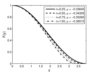
Figure 1. The similarity profiles $F(y)$ of (1.20) for $N=1$ in four cases $n=\frac{1}{4}$, $\frac{1}{2}$, $\frac{3}{4}$ and $1$; $F(0)=1$, $\mu=F^{\prime\prime}(0)$.

First, for $n=1$, relying on the explicit representation (1.21) and good spectral properties of the corresponding self-adjoint linearised rescaled operator, we show that, for $p=p_{0}=2+\frac{4}{N}$, the TFE with absorption (1.5) admits asymptotic patterns of the following form:

(1.22) $$\textstyle{u(x,t)\sim(t\ln t)^{-\beta N}F_{*}(x/t^{\beta}(\ln t)^{-\beta N/4})\quad\left(\beta=\frac{1}{4+N}\right).}$$

Here $F_{*}$ is a fixed rescaled profile from the family (1.21) with a uniquely chosen parameter $a=a_{*}>0$ that depends on $N$ only. We also present evidence that similar logarithmic factors can occur for arbitrary $n>0$ but this does not lead to self-adjoint linearised operators and explicit mathematics. On the other hand, for the semilinear case $n=0$, i.e., for the fourth-order parabolic equation written for solutions of changing sign

(1.23) $$u_{t}=-\Delta^{2}u-|u|^{p-1}u,$$

the critical behaviour like (1.22) is known to occur at the critical exponent $p=1+\frac{4}{N}$ [21], which is precisely (1.6) with $n=0$. In this case, the centre manifold analysis also uses spectral properties of a non self-adjoint linear operator studied in [13, Sect. 2].

In Section 3 we briefly describe the essence of the easier supercritical case $p>p_{0}$. Very singular similarity solutions (VSSs) in the subcritical one $p\in(n+1,p_{0})$ will be studied in a forthcoming paper.

In Section 4, we explain how the critical asymptotic behaviour occurs for the $2m$th-order TFE with absorption

(1.24) $$u_{t}=(-1)^{m+1}\nabla\cdot(u^{n}\nabla\Delta^{m-1}u)-u^{p},\quad m\geq 2,$$

where the critical absorption exponent is

(1.25) $$\textstyle{p_{0}=1+n+\frac{2m}{N},}$$

and again $n=1$ leads to a simpler self-adjoint case.

In Section 5 we discuss similar local and global asymptotics for the Cauchy problem admitting maximal regularity solutions of changing sign.

Finally, let us note that (1.6) (and (1.25) for equation (1.24)) is the critical Fujita exponent of the TFE with source

$$u_{t}=-\nabla\cdot(|u|^{n}\nabla\Delta u)+|u|^{p}\quad(n>0,\,\,p>1),$$

i.e., for $p\in(n+1,p_{0}]$, all solutions with arbitrarily small initial data $u_{0}(x)$, where $\int u_{0}>0$, blow-up in finite time, [23].

2. Rescaled equation and centre subspace behaviour

2.1. To the style of the analysis

For convenience of the Reader, we must emphasize from the beginning that all our final conclusions on centre subspace behaviours detected below are mathematically formal when we deal with the quasilinear case $n>0$. The semilinear case $n=0$ is easier and admits a rigorous treatment by invariant manifold theory, [21]. It is then worth mentioning that there is no hope that such asymptotics can admit a reasonably simple rigorous treatment. We recall that even for the second-order model (1.15) with $n>0$, there is no a full centre manifold justification of the main results that were proved by essential use of the Maximum Principle and comparison-barrier techniques; see [25, Ch. 4]. Some of asymptotic patterns for (1.15) of centre subspace type turned out to be very complicated, [22]. As we will show, the main difficulty is not a proper spectral theory of linearized operators (this is justified in many cases) but a justification of the centre subspace behaviour associated with such singular operators. On the other hand, we always clearly indicate the rigorous steps and split the whole approaches into a sequence of standard steps. We would be very pleased if some of our formal results and discussions would attract attention of experts in these areas of differential equations.

Thus, in what follows, we use by implication the following rule:

(i) all conclusions concerning spectral and other properties of self-adjoint singular elliptic and ordinary differential operators are rigorous (or can be made rigorous after sometimes technical manipulations; for non-self-adjoint cases we are not that certain and extra analysis is necessary); and

(ii) further extensions via above spectral properties to describe the behaviour for TFEs close to center subspaces and various matching procedures are mathematically formal.

2.2. Rescaled equation

We begin with rescaling the PDE (1.5) with the critical exponent (1.6) according to the time-factors of the source-type solution (1.19), i.e., by setting

(2.1) $$u(x,t)=(1+t)^{-\beta N}v(y,\tau),\quad y=x/(1+t)^{\beta},\quad\tau=\ln(1+t),$$

that leads to the following autonomous rescaled equation in $\mathbb{R}^{N}\times\mathbb{R}_{+}$:

(2.2) $$v_{\tau}={\bf A}(v)-v^{p},$$

where ${\bf A}$ is the operator specified in (1.20). We first need to check that a simple stabilization as $\tau\to+\infty$ to a nontrivial stationary solution in (2.2) is not possible.

Proposition 2.1.

The stationary equation

(2.3) $${\bf A}(g)-g^{p}=0$$

does not have a nontrivial compactly supported nonnegative solution of the FBP.

Proof. Indeed, integrating (2.3) over ${\rm supp}\,g$ yields $\textstyle{\int g^{p}(y)\,{\mathrm{d}}y=0.}\quad\mbox{$\qed$}$

This means that the only bounded nonnegative equilibrium for the dynamical system (2.2) is trivial,

(2.4) $$g(y)\equiv 0\quad\mbox{in}\,\,\,\mathbb{R}^{N}.$$

In order to detect the actual non-stationary asymptotic behaviour, we next perform second rescaling by introducing the as yet unknown positive function $b(\tau)$,

(2.5) $$v(y,\tau)=b(\tau)w(\zeta,\tau),\quad\zeta=y/b^{\frac{n}{4}}(\tau),$$

to get the following perturbed equation:

(2.6) $$\textstyle{w_{\tau}={\bf A}(w)+\frac{b^{\prime}}{b}\,{\bf C}w-b^{p-1}w^{p},\quad\mbox{where}\,\,\,{\bf C}w\equiv\frac{n}{4}\,\nabla w\cdot\zeta-w.}$$

2.3. Linearisation

Roughly speaking, in order to detect the asymptotic behaviour according to (2.5), we can use the estimate

(2.7) $$b(\tau)\approx\|v(\cdot,\tau)\|_{\infty}\to 0\quad\mbox{as}\,\,\,\tau\to\infty,$$

so that $\|w(\cdot,\tau)\|_{\infty}\approx 1$ for $\tau\gg 1$. On the other hand, in the radial setting, it is convenient to use $b(\tau)$ for the scaling of the support of the solution $w(\zeta,\tau)$ to get that it approaches the unit ball $B_{1}$ as $\tau\to\infty$; see below.

We next perform the linearisation by setting

(2.8) $$w(\zeta,\tau)=F(\zeta)+Y(\zeta,\tau),$$

where $F$ is a rescaled similarity profile from the family (1.21). Then $Y$ solves the following rescaled equation:

(2.9) $$\textstyle{Y_{\tau}={\bf A}^{\prime}(F)Y+\frac{b^{\prime}}{b}\,{\bf C}F-b^{p-1}F^{p}+{\bf D}(Y)-b^{p-1}[(F+Y)^{p}-F^{p}],}$$

where ${\bf A}^{\prime}(F)Y$ is the formal Frechet derivative of ${\bf A}$ at $F$,

(2.10) $${\bf A}^{\prime}(F)Y=-\nabla\cdot(F^{n}\nabla\Delta Y)-\nabla\cdot(nF^{n-1}Y\nabla\Delta F)+\beta\nabla Y\cdot y+\beta NY,$$

and ${\bf D}(Y)$ is a higher-order perturbation, which is quadratic in $Y\to 0$ on smooth functions. Using the elliptic equation (1.20) for $F$, on integration,

(2.11) $$F^{n}\nabla\Delta F=\beta Fy\quad\Longrightarrow\quad{\bf A}^{\prime}(F)Y=-\nabla\cdot(F^{n}\nabla\Delta Y)+(1-n)\beta\nabla\cdot(Y\zeta).$$

2.4. The self-adjoint case $n=1$

It follows from (2.11) that $n=1$ is a special case, where the last term vanishes. We fix $a=1$ in (1.21), so that the linearised operator is

(2.12) $${\bf A}^{\prime}(F)Y=-\nabla\cdot(F\nabla\Delta Y)\equiv-c_{0}\nabla\cdot((1-|\zeta|^{2})\nabla\Delta Y),\quad y\in B_{1}=\{|\zeta|<1\}.$$

One can see that it can be written in the form

(2.13) $$\textstyle{{\bf A}^{\prime}(F)Y=-c_{0}\frac{1}{\rho(|\zeta|)}\,[\Delta(a(|\zeta|)\Delta Y)+2N\Delta Y],\quad\mbox{where}\,\,\,a(|\zeta|)=1-|\zeta|^{2}=\frac{1}{\rho(|\zeta|)},}$$

so, in the topology of $L^{2}_{\rho}(B_{1})$, operator (2.12) is symmetric in $C^{\infty}_{0}(B_{1})$ with good coefficients, and hence admits self-adjoint extensions. Next, using classical theory [10], we specify properties of its unique Friedrichs self-adjoint extension. Its domain is constructed by completing $C^{\infty}_{0}(B_{1})$ in the norm induced by its positive quadratic form (corresponding to the operator $-{\bf A}^{\prime}(F)-c_{0}\Delta>0$)

$$\textstyle{\langle Y,W\rangle_{*}\equiv c_{0}\int_{B_{1}}[a\Delta Y\Delta W-(2N-1)\nabla Y\cdot\nabla W].}$$

The intersection of this Hilbert space with the domain of the maximal adjoint operator $D(({\bf A}^{\prime}(F))^{*})=\{v\in L^{2}_{\rho}:\,\,{\bf A}^{\prime}(F)v\in L^{2}_{\rho}\}$ defines the domain of the self-adjoint extension, which we denote by $D({\bf A}^{\prime}(F))=H^{4}_{\rho,0}$. In particular, for any $v\in H^{4}_{\rho,0}$, there holds

$$\textstyle{v=0\quad\mbox{on}\,\,\,\partial B_{1},\quad\mbox{and}\quad\int_{B_{1}}a(\Delta v)^{2}<\infty,}$$

so that $H^{4}_{\rho,0}\subset H^{2}_{\rho,0}$. Consider the corresponding eigenvalue problem written in the form

(2.14) $$-c_{0}[\Delta(a(|\zeta|)\Delta\psi)+2N\Delta\psi]=\rho\lambda\psi\quad\mbox{in}\,\,\,H^{4}_{\rho,0}.$$

Since the embeddings of the corresponding functional spaces $H^{2}_{a,0}$ and $H^{1}_{0}$ into $L^{2}_{\rho}$ are compact, [35, p. 63], we have that the spectrum $\sigma({\bf A}^{\prime}(F))$ is real and discrete.

For our purposes, it suffices to detect the eigenvalues and eigenfunctions in the radial (ODE) setting with the single spatial variable $r=|\zeta|>0$. The extension to the elliptic setting is performed by using the polar coordinates $\zeta=(r,\sigma)$ in $B_{1}$,

(2.15) $$\Delta=\Delta_{r}+\mbox{$\frac{1}{r^{2}}$}\,\Delta_{\sigma},$$

where $\Delta_{\sigma}$ is the Laplace-Beltrami operator on the unit sphere $S^{N-1}=\partial B_{1}$ in $\mathbb{R}^{N}$. $\Delta_{\sigma}$ is a regular operator with a discrete spectrum in $L^{2}(S^{N-1})$ (each eigenvalue repeated as many times as its multiplicity),

(2.16) $$\sigma(-\Delta_{\sigma})=\{\nu_{k}=k(k+N-2),\,\,k\geq 0\},$$

and an orthonormal, complete, closed subset $\{V_{k}(\sigma)\}$ of eigenfunctions, which are homogeneous harmonic $k$-th order polynomials restricted to $S^{N-1}$. We plug (2.15) into (2.13), where all the coefficients are radial functions, and use the separation of variables

(2.17) $$\psi(r,\sigma)=R(r)V_{k}(\sigma)$$

for solving the eigenvalue problem (2.14). For each fixed $\nu_{k}$, we then arrive at a radial eigenvalue problem for $R$, which is similar to that discussed below.

Thus we take $k=0$ in (2.17) and consider the radially symmetric eigenvalue problem (2.14). For $N=1$, this problem was studied in [8], where further references are given. It is not difficult to check that the radial operator ${\bf A}^{\prime}(F)$ has the discrete spectrum

(2.18) $$\sigma({\bf A}^{\prime}(F))=\{\lambda_{k}=c_{0}k(k+2)(k+N)(k+N+2),\,\,\,k=0,2,4,...\},$$

where each eigenfunction $\psi$ is a ($k$+2)th-order polynomial,

(2.19) $$\psi_{k}(r)=b_{k}(r^{k+2}+...+d_{k})\quad(\psi_{k}(1)=0),$$

where $\{b_{k}\}$ are normalization constants, so that the eigenfunction subset $\{\psi_{k}\}$ is orthonormal in $L^{2}_{\rho}$. In particular,

(2.20) $$\textstyle{\psi_{0}(r)=b_{0}(r^{2}-1)>0,\quad b_{0}=-\sqrt{\frac{N+2}{2\omega_{N}}}\quad(\lambda_{0}=0),}$$

where $\omega_{N}=\frac{2\pi^{N/2}}{N\Gamma(N/2)}$ is the volume of the unit ball in $\mathbb{R}^{N}$. Such polynomials are complete and closed in typical weighted $L^{p}$-spaces (a standard functional analysis result; see [13, Sect. 2.3] for details), and this justifies the equality in (2.18). Moreover, we then can use the eigenfunction expansion with the orthonormal eigenfunctions subset $\{\psi_{k}\}$ to deal with solutions of the corresponding PDE.

We next consider the rescaled equation (2.9), which for $n=1$ takes the form

(2.21) $$\textstyle{Y_{\tau}={\bf A}^{\prime}(F)Y+\frac{b^{\prime}}{b}\,{\bf C}F-b^{p-1}F^{p}-\nabla\cdot(Y\nabla\Delta Y)-b^{p-1}[(F+Y)^{p}-F^{p}].}$$

We deal with strong radially symmetric solutions of (2.21), where we now choose the normalization function $b(\tau)$ in (2.5) such that

(2.22) $${\rm supp}\,w(\cdot,\tau)=B_{1}\quad\mbox{for}\,\,\,\tau\gg 1.$$

According to equation (2.21), we then need to assume that $b(\tau)$ is smooth, at least, for large $\tau$, though this requirement can be weaken by using a weak (integral) form of the PDE. We now use the converging (in $L^{2}_{\rho}$ and in the corresponding Sobolev class) eigenfunction expansion of the radial solution

(2.23) $$\textstyle{Y(\zeta,\tau)=\sum_{k\geq 0}a_{k}(\tau)\psi_{k}(\zeta)}$$

to study the corresponding centre subspace behaviour for the nonlinear operator ${\bf A}$. This part of our asymptotic analysis is formal.

Thus substituting (2.23) into (2.21) and projecting onto $\psi_{0}$ in $L^{2}_{\rho}$, we have that the first coefficient satisfies the following perturbed “ODE”:

(2.24) $$\textstyle{a_{0}^{\prime}=-\gamma_{1}\frac{b^{\prime}}{b}-\gamma_{2}b^{p-1}+...\,},\,\,\,\mbox{where}\,\,\,\gamma_{1}=-\langle{\bf C}F,\psi_{0}\rangle_{\rho}>0,\,\,\gamma_{2}=\langle F^{p},\psi_{0}\rangle_{\rho}>0.$$

We omit in (2.24) the higher-order terms assuming that, for this type of behaviour, the non-autonomous perturbations are the leading ones. The signs of the coefficients $\gamma_{1,2}$ in (2.24) are essential and are easily checked by integration.

It follows from (2.4) and (2.22) that $b(\tau)\to 0$ as $\tau\to\infty$, so

$$\frac{b^{\prime}(\tau)}{b(\tau)}\quad\mbox{is not integrable at $\tau=\infty$}.$$

Therefore, in order to have a uniformly bounded expansion coefficient $a_{0}(\tau)$, we need to suppose that two terms on the right-hand side of (2.24) annul each other asymptotically, so that, up to an integrable perturbation,

(2.25) $$\textstyle{\frac{b^{\prime}}{b}=-\frac{\gamma_{2}}{\gamma_{1}}\,b^{p-1}+...\quad\mbox{for}\,\,\,\tau\gg 1.}$$

This gives the following necessary condition for existing of such a behaviour:

(2.26) $$\textstyle{b(\tau)=\gamma_{*}\tau^{-\frac{1}{p-1}}+...\,,\quad\mbox{where}\,\,\,\gamma_{*}=\bigl{[}\frac{(p-1)\gamma_{2}}{\gamma_{1}}\bigr{]}^{-\frac{1}{p-1}}.}$$

Returning to the original variables $\{x,t,u\}$, from (2.26) we obtain the asymptotic pattern (1.22). The rescaled profile $F_{*}$ is uniquely determined from (1.21) with $a_{*}=\gamma_{*}^{n/4}$.

2.5. Arbitrary $n\in(0,\frac{3}{2})$.

This non self-adjoint case is more difficult. Consider the linearised operator (2.11) for $n\not=1$, where $F>0$ is the radial solution of the ODE (1.20) in $B_{1}$; see [20] for existence, uniqueness, and asymptotics. Then, for $n<\frac{3}{2}$ [20],

(2.27) $$F(\zeta)\sim(1-|\zeta|)^{2}\quad\mbox{as}\,\,\,|\zeta|\to 1^{-}.$$

Notice that there exists a one-parameter family of the solutions given by

(2.28) $$\textstyle{F_{a}(\zeta)=a^{\frac{4}{n}}F(\frac{\zeta}{a}),\quad a>0.}$$

Firstly, we claim that, for $n\neq 1$, operator (2.11) is not symmetric in $L^{2}_{\rho}$ for any positive weight $\rho$ in $B_{1}$; see Appendix A. Secondly, we have that

(2.29) $$\textstyle{\psi_{0}(\zeta)=\frac{\mathrm{d}}{{\mathrm{d}}a}F_{a}(\zeta)|_{a=1}\equiv\frac{4}{n}\,F-\nabla F\cdot\zeta}$$

is a positive eigenfunction of (2.11) corresponding to $\lambda_{0}=0$. Observe that, with respect to the regularity, this eigenfunction well corresponds to that for $n=1$; cf. (2.20). Moreover, it follows that, close to the singular point $|\zeta|=1$, the radial part of (2.11) is governed by the singular (at $\partial B_{1}$) higher-order operator

(2.30) $$L_{4}Y=-(s^{2n}Y^{\prime\prime\prime})^{\prime},\quad s=1-|\zeta|,$$

which is symmetric in a weighted $H^{-1}$ topology (but we need a result in $L^{2}$). Solving the problem $L_{4}Y=g$ with natural conditions at the point $s=1$, which is assumed to be regular, we obtain, up to compact perturbations, that

(2.31) $$\textstyle{L_{2}Y\equiv-Y^{\prime\prime}\sim\int^{s}s^{-2n}\int^{s}g\equiv L_{*}g\quad\Longrightarrow\quad Y\sim L_{2}^{-1}L_{*}g,}$$

where $L_{2}^{-1}$ is a compact operator in $L^{2}$. It is easy to check that the integral operator $L_{*}$ is bounded in $L^{2}$ for

(2.32) $$\textstyle{n<\frac{3}{4},}$$

and then $L_{2}^{-1}L_{*}$ is compact in $L^{2}$ as the product of a compact and a bounded operator. Therefore ${\bf A}^{\prime}(F)$ has discrete spectrum in the parameter range (2.32). This is not an optimal result since, as we have seen, the discreteness of the spectrum remains valid for $n=1$. We use this analysis as a simple illustration of the fact that the spectrum is usually discrete in the non-symmetric case.

Thus $0\in\sigma({\bf A}^{\prime}(F))$ is an isolated eigenvalue. There is a numerical evidence that the spectrum is discrete for all $n\in(0,\frac{3}{2})$; see [8], where, moreover, first six eigenvalues turned out to be real for $N=1$. Possibly this might mean that in a special topology of sequences as $l^{2}$ (not related to any of $L^{2}_{\rho}$) the linearised operator can be treated as symmetric and self-adjoint; cf. an example in [13]. For $n=0$ in any dimension $N\geq 1$, the whole spectrum is proved to be real. We refer to [13, Sect. 2], where this and other $2m$th-order operators were studied in $L^{2}_{\rho}(\mathbb{R}^{N})$, i.e., for the Cauchy (not a free-boundary) problem.

The rest of our study is formal. Once in the radial setting there exists the centre subspace of ${\bf A}^{\prime}(F)$, we are looking for a (formal) centre subspace patterns for (2.9)

(2.33) $$Y(\zeta,\tau)=a_{0}(\tau)\psi_{0}(\zeta)+...\,.$$

We assume the centre subspace dominance in the behaviour, so, as usual, other terms in this expansion are assumed to be negligible for $\tau\gg 1$. Substituting (2.33) into (2.9), we next find the projection onto the corresponding adjoint eigenfunction $\psi_{0}^{*}$. In general, such an analysis becomes rigorous if we establish existence of complete, closed and bi-orthonormal eigenfunction subsets $\{\psi_{k}\}$ and $\{\psi_{k}^{*}\}$. This is an open problem except the case $n=1$ above and $n=0$ studied in [13]. We do not deal with the adjoint operator ${\bf A}^{\prime*}(F)$ in this formal asymptotic analysis. The projection onto $\psi_{0}^{*}$ yields the perturbed ODE (2.24), where the same coefficients $\gamma_{1,2}$ are determined via the standard dual $L^{2}$ product, where $\psi_{0}$ is replaced by $\psi_{0}^{*}$. This formally leads to the same asymptotics (2.26).

The range $n\in[\frac{3}{2},3)$. The centre subspace analysis applies also for larger $n$’s. The asymptotics of similarity profiles change at $n=\frac{3}{2}$, where, instead of (2.27),

(2.34) $$F(\zeta)\sim(1-|\zeta|)^{2}\bigl{[}\frac{3}{4}\,\beta|\ln(1-|\zeta|)|\bigr{]}^{\frac{2}{3}}\quad\mbox{as}\,\,\,|\zeta|\to 1;$$

see [20]. On the other hand, for $n\in(\frac{3}{2},3)$,

(2.35) $$F(\zeta)\sim(1-|\zeta|)^{\frac{3}{n}}\quad\mbox{as}\,\,\,|\zeta|\to 1.$$

This regularity is sufficient for determining the corresponding eigenfunction and the logarithmic behaviour.

For $n\geq 3$, the zero contact angle FBP does not provide us with a proper interesting evolution; see [20].

3. On the supercritical parameter range $p>p_{0}$

3.1. Exponentially perturbed dynamical system for $p>p_{0}$

Let us explain what we expect for $p>p_{0}$ in (1.5). In terms of the rescaled function

(3.1) $$u(x,t)=(1+t)^{-\frac{N}{4+nN}}v(y,\tau),\quad\tau=\ln(1+t),$$

the equation takes the form

(3.2) $$\textstyle{v_{\tau}=-\nabla\cdot(v^{n}\nabla\Delta v)+\frac{1}{4+nN}\,y\cdot\nabla v+\frac{N}{4+nN}\,v-{\mathrm{e}}^{-\gamma\tau}v^{p},}$$

where $\gamma=\frac{N(p-p_{0})}{4+nN}>0$ if $p>p_{0}$. Therefore the absorption term $-u^{p}$ in (1.5) generates an exponentially small perturbation in the rescaled equation (3.2). Hence one can expect the convergence as $\tau\to\infty$ to the rescaled similarity profile $F$ in (1.19) of the limit mass, though the passage to the limit in (3.2) generates a number of technical difficulties. Here (3.2) is formally an exponentially small perturbation of the autonomous rescaled TFE

(3.3) $$\textstyle{v_{\tau}={\bf A}(v)\equiv-\nabla\cdot(v^{n}\nabla\Delta v)+\frac{1}{4+nN}\,y\cdot\nabla v+\frac{N}{4+nN}\,v}.$$

As usual, we gain an extra advantage in the case $n=1$.

3.2. The gradient case $n=1$

It is known that, for $n=N=1$, the rescaled TFE (3.3) is a gradient system, [12]. Let us construct an “approximate” Lyapunov function for strong solutions of the FBP in $\mathbb{R}^{N}$. Namely, we write down (3.2) in the form

(3.4) $$\textstyle{v_{\tau}=\nabla\cdot\bigl{[}v\nabla\bigl{(}-\Delta v+\frac{1}{2(4+N)}\,|y|^{2}\bigr{)}\bigr{]}+{\mathrm{e}}^{-\gamma\tau}v^{p}}$$

and multiply in $L^{2}(\mathbb{R}^{N})$ by $(-\Delta_{v})^{-1}v_{\tau}$, where, by definition,

$$(-\Delta_{v})^{-1}w=g\quad\mbox{if}\,\,\,\Delta_{v}g\equiv\nabla\cdot(v\nabla g)=-w,$$

and $g=0$ at the free boundary of $v$. Then integrating by parts yields the identity

(3.5) $$\textstyle{\int v|\nabla(-\Delta_{v})^{-1}v_{\tau}|^{2}=\frac{{\mathrm{d}}}{{\mathrm{d}}\tau}\,\bigl{[}-\frac{1}{2}\,\int|\nabla v|^{2}-\frac{1}{2(4+N)}\,\int v|y|^{2}\bigr{]}+J,}$$

where $J$ corresponds to the exponentially small term,

(3.6) $$\textstyle{J={\mathrm{e}}^{-\gamma\tau}\int v^{p}(-\Delta_{v})^{-1}v_{\tau}.}$$

Integrating (3.5) over $(0,T)$ yields

$$\int_{0}^{T}\int v|\nabla(-\Delta_{v})^{-1}v_{\tau}|^{2}+\frac{1}{2}\,\int|\nabla v(T)|^{2}+\frac{1}{2(4+N)}\,\int v(T)|y|^{2}\bigr{]}\leq C+\int_{0}^{T}J,$$

so that, if the exponential term (3.6) $J\in L^{1}(\mathbb{R}_{+})$, this yields extra uniform estimates,

$$\sqrt{v}\,\nabla(-\Delta_{v})^{-1}v_{\tau}\in L^{2}(\mathbb{R}\times\mathbb{R}_{+})\,\,\,\mbox{and}\,\,\,\nabla v,\,\sqrt{v}|y|\in L^{\infty}(\mathbb{R}_{+};L^{2}).$$

Note that, obviously, (3.5) does not imply existence of a Lyapunov function (the non-autonomous PDE (3.4) is not a gradient system). Anyway, since (3.5) gives a rather strong estimate of $v_{\tau}$ for $\tau\gg 1$, this makes it possible to pass to the limit $\tau\to\infty$ and establish stabilization to an equilibrium point (see the technique in [25, p. 116-117]), which is unique by the obvious mass-monotonicity with time of the solution.

The symmetry of the Frechet derivative (2.12) at $F$ looks like a certain “remnant” of the fact that the original PDE is a gradient system.

4. Centre subspace patterns for the $2m$th-order TFE

We consider the $2m$th-order TFE with absorption (1.24) with the critical absorption (Fujita) exponent (1.25). The proper setting of a standard “zero contact angle” FBP for the TFE includes $m$+1 free boundary conditions at the free boundary $\Gamma_{0}=\partial\Omega(t)\times\mathbb{R}_{+}$ ($\Omega(t)$ is the support of $u(\cdot,t)$ at time $t>0$),

(4.1) $$\textstyle{u=\nabla u=...=\frac{\partial^{m-1}u}{\partial{\bf\nu}^{m-1}}={\bf\nu}\cdot\nabla(u^{n}\Delta^{m-1}u)=0,}$$

where $\nu$ is the unit outward normal to $\partial\Omega(t)$ that is assumed to be sufficiently smooth.

4.1. Similarity solutions

The similarity solutions of the pure TFE

(4.2) $$u_{t}=(-1)^{m+1}\nabla\cdot(u^{n}\nabla\Delta^{m-1}u)$$

take the standard form (1.19) with

(4.3) $$\textstyle{\beta=\frac{1}{2m+nN}.}$$

One can see that the critical exponent (1.25) is precisely the one, for which the PDE (1.24) possesses the same group of scaling transformation. Then the rescaled profile $F$ satisfies the radial restriction of the $2m$th-order elliptic equation

(4.4) $${\bf A}(F)=(-1)^{m+1}\nabla\cdot(F^{n}\nabla\Delta^{m-1}F)+\beta\nabla F\cdot y+\beta NF=0.$$

It seems that, for any $m\geq 3$, the questions of existence and uniqueness of a solution $F(y)>0$ in $B_{1}$ remain open. It is clear that, for large $m$, a standard approach to existence based on a multi-parametric shooting leads to a complicated geometric analysis (though some general conclusions in this geometry are likely). We expect that the approach based on the $n$-branching (or a continuous homotopy connection with $n=0$) via the classical theory [42] makes it possible to explain properties solutions, at least, for small $n>0$ by branching from the linear case $n=0$ (but, surely, a standard approach to smooth branching does not apply). For the Cauchy problem, the spectral and other properties of the corresponding linear operator (4.4) for $n=0$ are given in [13], and can be used to clarify the behaviour for small $n>0$. For the FBP (4.1), an extra analysis of the linearised elliptic PDE is necessary.

As usual, the case $n=1$ provides us with the explicit solution. Writing the ODE (4.4) in the radial divergent form (here $y$ is actually $|y|$)

$$(y^{N-1}F(\Delta^{m-1}F)^{\prime})^{\prime}=(-1)^{m}\beta(y^{N}F)^{\prime},$$

on integration we obtain $\Delta^{m-1}F=(-1)^{m}\frac{1}{2}\,\beta y^{2}$. Integrating this linear ODE $2m$-2 times yields the positive solution in $B_{1}$

(4.5) $$\textstyle{F(y)=c_{0}(1-|y|^{2})^{m},\quad\mbox{where}\,\,\,c_{0}=\frac{1}{2}\,\frac{N!!}{(2m)!!(2m+N)!!}.}$$

4.2. Linearised operator

We next follow the same scheme of the asymptotic analysis as in Section 2. Similar to (2.10), we introduce the linearised operator

(4.6) $${\bf A}^{\prime}(F)Y =(-1)^{m+1}\nabla\cdot(F^{n}\nabla\Delta^{m-1}Y)$$

$$+\,(-1)^{m+1}\nabla\cdot(nF^{n-1}Y\nabla\Delta^{m-1}F)+\beta\nabla Y\cdot y+\beta NY.$$

Using the ODE (4.4), we have that

$$(-1)^{m+1}\nabla\cdot(nF^{n-1}\nabla\Delta^{m-1}F)=-\beta nN,\,\,\,(-1)^{m+1}nF^{n-1}\nabla\Delta^{m-1}F=-\beta ny,$$

so (4.6) can be written in the form

(4.7) $${\bf A}^{\prime}(F)Y=(-1)^{m+1}\nabla\cdot(F^{n}\nabla\Delta^{m-1}Y)+\beta N(1-n)y\cdot\nabla Y+\beta N(1-n)Y,$$

and we again observe that $n=1$ is a special case.

4.3. The self-adjoint case $n=1$

Plugging the profile (4.5) into (4.7) yields the following symmetric form of the operator:

(4.8) $${\bf A}^{\prime}(F)Y =c_{0}(-1)^{m+1}\nabla\cdot((1-|y|^{2})^{m}\nabla\Delta^{m-1}Y)$$

$$\equiv\,c_{0}(-1)^{m+1}[D^{m}((1-|y|^{2})D^{m}Y)+m(m-1)N\Delta^{m-1}Y],$$

where $D^{m}$ denotes $\Delta^{m/2}$ for $m$ even and $\nabla\Delta^{(m-1)/2}$ for $m$ odd. For instance, for $N=1$ and $m=3$, we have

$${\bf A}^{\prime}(F)Y=c_{0}(1-y^{2})^{2}[((1-y^{2})Y^{\prime\prime\prime})^{\prime\prime\prime}+6Y^{(4)}].$$

Having the symmetric operator (4.8) in $C^{\infty}_{0}$, we next determine its self-adjoint extensions, [10]. In particular there exists the extension with discrete spectrum and polynomial eigenfunctions in the radial setting (the non-radial case is covered by using the spherical polynomials as in (2.17)). The eigenvalues $\lambda_{k}$ for the polynomials $\psi_{k}(y)$ given in (2.19) are calculated by using (4.8),

(4.9) $$\lambda_{k}=-c_{0}(k+2)k...[k+2-2(m-2)](k+N+2)(k+N)...[k+N-2(m-2)]$$

for $k=2(m-3),2(m-2),...\,.$ Using the eigenfunction expansion in terms of complete and closed subset of polynomials $\{\psi_{k}\}$ partially justifies the asymptotic centre subspace analysis of the corresponding rescaled equation (2.9), which yields the same ODE (2.24) and hence the asymptotics (2.26). Here in the critical case (1.25) we still have $\frac{1}{p-1}=\beta N$ with $\beta$ given by (4.3). Finally, we arrive at the asymptotic pattern (1.22), where $4$ is replaced by $2m$.

4.4. The general case $n\not=1$

We do not have such a self-adjoint operator, but anyway, once $F>0$ in $B_{1}$ is determined, we obtain the radial eigenfunction $\psi_{0}$ for $\lambda_{0}=0$ from the scaling symmetry group (2.28) (the exponent $\frac{4}{n}$ is replaced by $\frac{2m}{n}$) of equation (4.4). We can also guarantee that (4.7) has compact resolvent provided that $n>0$ is not large, so $\lambda_{0}=0$ is an isolated eigenvalue. The rest of the centre subspace behaviour via the expansion (2.33) remains unchanged and leads to similar logarithmically perturbed asymptotic patterns. A rigorous justification is a hard open problem.

5. Logarithmically perturbed patterns in the Cauchy problem

The asymptotic behaviour and similarity solutions for the TFE (1.12) or (1.24) posed in the whole space $\mathbb{R}^{N}\times\mathbb{R}_{+}$ are less studied in thee literature. For $n\in(0,\frac{3}{2})$, in the Cauchy problem (CP), the solutions exhibiting the “maximal regularity” at the interfaces are oscillatory and of changing sign. See [17, 18] and the book [24, Ch. 1] for correct meaning of the CP for thin film equations and further examples. For such solutions, we need to assume that $u^{n}$ in (4.1) is replaced by $|u|^{n}$. Therefore from now on in all the expressions and equations we use the convention that

(5.1) $$\begin{gathered}u^{n},f^{n},v^{n},w^{n},...\,\,\,\mbox{are replaced by}\,\,\,|u|^{n},|f|^{n},|v|^{n},|w|^{n},...\,\,\,\mbox{and},\\ u^{p},f^{p},v^{p},w^{p},...\,\,\,\mbox{are replaced by}\,\,\,|u|^{p-1}u,|f|^{p-1}f,|v|^{p-1}v,|w|^{p-1}w,...\,.\end{gathered}$$

We must admit that solutions of changing sign are less relevant for many known physical applications of TFEs. Nevertheless, for general PDE theory, it is key and of principal importance to include the Cauchy problem and to show that the basic techniques developed above apply to these much more complicated oscillatory solutions.

The idea of sign changing solutions of TFEs is straightforward. Indeed, the oscillatory properties of such solutions are a manifestation of the fact that TFEs (4.2) are “homotopic”, i.e., can be continuously deformed (e.g., as $n\to 0$) via non-singular uniformly parabolic PDEs with analytic coefficients (see details in [18, Sect. 14]) to the linear poly-harmonic equation

(5.2) $$u_{t}=(-1)^{m+1}\Delta^{m}u\quad\mbox{in}\,\,\,\mathbb{R}^{N}\times\mathbb{R}_{+}.$$

By classical parabolic theory (see e.g. Eidel’man [14]), given initial data $u_{0}\in L^{1}$, there exists the unique solution of the Cauchy problem for (5.2) defined by the convolution

(5.3) $$u(x,t)=b(x,t)*u_{0},\quad b(x,t)=t^{-\frac{N}{2m}}F(y),\,\,\,y=x/t^{\frac{1}{2m}},$$

where $b(x,t)$ is the fundamental solution of the operator $D_{t}-(-1)^{m+1}\Delta^{m}$. For any $m\geq 2$, the rescaled kernel $F=F(|y|)$ is oscillatory as $y\to\infty$, so this property of changing sign is inherited by $L^{1}$ solutions of (5.2). Assuming a continuous (homotopic) deformation of a class of solutions of (1.12) as $n\to 0^{+}$, this confirms that the TFE admits oscillatory solutions of changing sign at least for not that large $n>0$. Continuity and homotopy concepts are effective for treating the Cauchy problem for higher-order TFEs; see other examples in [18].

Then the source-type solutions of the TFE take the same form (1.19), where the radial function $F$ of changing sign solves the ODE (1.20) with the convention (5.1). We begin with the linear case $n=0$, which by continuity is going to describe some properties of source-type solutions for sufficiently small $n>0$.

5.1. Properties of the rescaled fundamental solution for $n=0$

The linear ODE

(5.4) $$\textstyle{{\bf A}(F)\equiv-\Delta^{2}F+\frac{1}{4}\,\nabla F\cdot y+\frac{N}{4}\,F=0\quad\mbox{in}\,\,\,\mathbb{R}^{N}}$$

is precisely the elliptic equation for the rescaled kernel $F$ of the fundamental solution in (5.3). Therefore the similarity profile $F(y)$ exists and is unique under the assumption

(5.5) $$\textstyle{\int F(y)\,{\mathrm{d}}y=1}$$

(in view of existence-uniqueness of the fundamental solution).

Let us next describe an important relation between similarity profiles for the FBP and the Cauchy problem. Without loss of generality, we consider the case $N=1$, where on integration once (5.4) takes the form

(5.6) $$F^{\prime\prime\prime}=\frac{1}{4}\,Fy.$$

It is easy to find all decaying profiles corresponding to the CP with the exponential WKBJ asymptotics as $y\to+\infty$,

(5.7) $$F(y)\sim y^{-\frac{1}{3}}{\mathrm{e}}^{ay^{4/3}},\quad\mbox{with $a$ satisfying}\,\,\,a^{3}=\frac{1}{4}\,(\frac{3}{4})^{3}.$$

There exist two complex conjugate roots for exponentially decaying profiles

(5.8) $$a_{\pm}=-\frac{3}{8}\,4^{-\frac{1}{3}}(1\pm{\rm i}\sqrt{3})\equiv-c_{1}\pm{\rm i}c_{2}.$$

This yields a two-dimensional bundle of oscillatory solutions with the behaviour

(5.9) $$F(y)\sim y^{-\frac{1}{3}}{\mathrm{e}}^{-c_{1}y^{4/3}}\bigl{[}A_{1}\cos\bigl{(}c_{2}y^{\frac{4}{3}}\bigr{)}+A_{2}\sin\bigl{(}c_{2}y^{\frac{4}{3}}\bigr{)}\bigr{]}\quad\mbox{as}\,\,\,y\to\infty,$$

where $A_{1}$ and $A_{2}$ are arbitrary constants. The algebraic factor $y^{-1/3}$ is obtained by a standard asymptotic WKBJ method. We observe here the periodic behaviour with a single fundamental frequency (a result we will refer to in the TFE analysis below).

Proposition 5.1.

For $N=1$, the rescaled profile of the Cauchy problem $F=F_{\infty}$ given by $(\ref{3.12})$, $(\ref{3.12.1})$ is the limit of FBP similarity profiles on bounded intervals,

(5.10) $$F_{\infty}=\lim F_{k},$$

where each $F_{k}(y)$ is defined on interval $(-y_{k},y_{k})$,

(5.11) $$F_{k}(\pm y_{k})=F_{k}^{\prime}(\pm y_{k})=0,\quad\mbox{and}$$

(5.12) $$y_{k}=\big{(}\frac{\pi}{c_{2}}\,k\big{)}^{\frac{3}{4}}(1+o(1))\quad\mbox{as}\,\,\,k\to\infty.$$

Proof. The geometric aspect of such a property is obvious in view of the oscillatory behaviour in (5.9). The convergence as $k\to\infty$ follows from straightforward computations related to the whole exponential bundle including (5.9) and the growing counterpart

$$F(y)=y^{-\frac{1}{3}}{\mathrm{e}}^{a_{0}y^{4/3}}+...\,,\quad\mbox{with}\,\,\,a_{0}=\frac{3}{4}\,4^{-\frac{1}{3}}.$$

Then solving the FBP problem (5.11) yields the asymptotic equality $\cos(c_{2}y_{k}^{4/3}+{\rm const.})=0,$ whence the asymptotics (5.12). ∎

We also expect the following Sturm property be valid:

(5.13) $$F_{k}(y)\quad\mbox{has precisely $k$ zeros on $(0,y_{k})$}.$$

Such a zero-number property is easily seen for $k\gg 1$, but is not obvious for smaller $k$’s.

5.2. Similarity profiles for $n>0$: existence and uniqueness

Proposition 5.2.

For $N=1$ and $n\in(0,1)$, the ODE $(\ref{Od11})$, $(\ref{Conv1})$ in $\mathbb{R}$ admits a unique solution $F\in C^{3}$ of unit mass. The solution $F(y)$ is symmetric, compactly supported and is oscillatory near finite interfaces at $y=\pm y_{0}$.

Proof. For $N=1$ the ODE (1.20) has the form

(5.14) $$|F|^{n}F^{\prime\prime\prime}=\beta Fy,\quad y\in\mathbb{R}.$$

Dividing by $|F|^{n}$ and setting $|F|^{-n}F=g$ yields

(5.15) $$(|g|^{\alpha}g)^{\prime\prime\prime}=\beta gy,\quad y\in\mathbb{R},\quad\alpha=\frac{n}{1-n}.$$

Then existence and uniqueness of a compactly supported solution $F\in C^{3}$ for any $n\in(0,1)$ follows from the results in Bernis–McLeod [6]. ∎

For $n\in[1,\frac{3}{2})$ solutions of (5.14) are less regular (see below), so the techniques in [6] do not apply directly, but we expect that the existence-uniqueness result remains valid and can be extended further to some interval $n\in[\frac{3}{2},n_{\rm h})$; see below.

In Figure 2 we have shown these similarity profiles for some $n>0$ including the linear case $n=0$ leading to the ODE (5.6) for the fundamental rescaled profile. Here we observe convergence of the fundamental profiles as $n\to 0^{+}$, which is justified rigorously if all the zeros are “transversal” and isolated except the last one; see below.

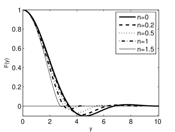
Figure 2. The oscillatory CP profiles satisfying (5.14). Parameters of shooting are $F^{\prime\prime}(0)=-0.3379890$ ($n=0$), $-0.3414702$ ($n=0.2$), $-0.3490986$ ($n=0.5$), $-0.3697143$ ($n=1$), and $-0.4052680$ ($n=1.5$).

5.3. Oscillatory properties via periodic orbits

We next describe the oscillatory properties of such changing sign profiles $F(y)$ near interfaces. We rescale $F$ to have that

$${\rm supp}\,F=[-1,1].$$

It was shown in [17] that the asymptotic behaviour of $F(y)$ satisfying (5.14) near the interface point $y\to 1^{-}$ is given by the expansion

(5.16) $$F(y)=(1-y)^{\mu}\phi(s),\quad s=\ln(1-y),\quad\mu=\frac{3}{n},$$

where, after scaling $\phi\mapsto\beta^{\frac{1}{n}}\phi$, the oscillatory component $\phi$ satisfies the following autonomous ODE (we omit exponentially small terms):

(5.17) $$\textstyle{\phi^{\prime\prime\prime}+3(\mu-1)\phi^{\prime\prime}+(3\mu^{2}-6\mu+2)\phi^{\prime}+\mu(\mu-1)(\mu-2)\phi+\frac{\phi}{|\phi|^{n}}=0.}$$

Oscillatory periodic orbits: existence. We are now interested in periodic solutions $\phi_{*}(s)$ of (5.17), which according to (5.16), can determine the simplest typical (and possibly stable and generic) oscillatory behaviour of solutions near interfaces when $s=\ln(1-y)\to-\infty$ as $y\to 1^{-}$. There are several classic methods of ODE theory for establishing existence and multiplicity of periodic solutions of finite-dimensional dynamical systems. These are various topological techniques, such as rotations of vector fields, index, and degree theory; see [32, Sect. 13, 14]. Another approach is based on branching theory, [42, Ch. 6]. In our case, such an $n$-branching approach is especially effective since for $n=0$ the unique solution $F$ is the rescaled kernel of the fundamental solution (a rigorous justification of some aspects of branching for such degenerate equations can be a hard problem). We also mention papers [43, 34, 31] containing further related references and methods concerning modern theory of periodic solutions of higher-order nonlinear ODEs. In general, equations like (5.17) are a difficult object to study, and especially the main difficulty is proving uniqueness of such periodic orbits. Therefore, later on, together with analytic techniques, we will need also to rely on careful numerical evidence on existence, uniqueness, and stability of periodic solutions.

It is curious that for $n=1$, the unique periodic solution can be detected by a direct algebraic approach; see [17, Sect. 7.4]:

Proposition 5.3.

For $n=1$, the ODE $(\ref{m=2.11})$ has a unique $T$-periodic solution, with

(5.18) $$T=-2\ln s>\theta=1.9248...\,,$$

where $\theta=0.381966...$ is the unique root on the interval $(0,1)$ of the cubic equation

(5.19) $$\theta^{3}-2\theta^{2}-2\theta+1=0.$$

Indeed, for $n=1$, the nonlinearity in (5.17) is ${\rm sign}\,\phi$ and the ODE is linear in the positivity and negativity domain of solutions,

$$\textstyle{\phi^{\prime\prime\prime}+6\phi^{\prime\prime}+11\phi^{\prime}+6\phi\pm 1=0,}$$

so can be solved explicitly. Matching positive and negative branches leads to the result.

Let us now state the main result concerning periodic orbits of the ODE (5.17).

Theorem 5.4.

The ODE $(\ref{m=2.11})$ admits a nontrivial stable periodic solution $\phi_{*}(s)$ of changing sign for all

(5.20) $$0<n<n_{\rm h}\in(\frac{3}{2},n_{\rm+}),\quad\mbox{where}\quad n_{\rm+}=\frac{9}{3+\sqrt{3}}=1.9019238...\,.$$

Uniqueness of such periodic $\phi_{*}(s)$ in the interval (5.20) is still open.

Proof. For the interval

(5.21) $$0<n<\frac{3}{2},$$

the proof of existence is performed in [17, p. 292] by a shooting argument. Numerical representation of periodic solutions is given therein on p. 294; see also [24, p. 143]. We need to point out the main two ingredients of the proof in [17]:

(i) it is shown that for exponents (5.21) no orbits of the dynamical system (DS) (5.17) are attracted to infinity as $s\to+\infty$, i.e., all orbits stay uniformly bounded; and

(ii) as a consequence, then (5.17) is a dissipative DS having a bounded absorbing set.

Dissipative DSs are known to admit periodic solutions in rather general setting [32, Sect. 39] provided these are non-autonomous (so the period is fixed). For the autonomous system (5.17), the proof in [17, Sect. 7.1] was completed by shooting. Note that, in view of the last term, (5.17) is not a smooth dynamical system and solutions are not locally $C^{3}$-smooth. Nevertheless, as shows local analysis [17, p. 291], at least for $n\in(0,2)$, the nonlinearity is integrable to guarantee local extensions of solutions through generic “transversal” zeros. This means that the equivalent integral equation is well-posed and is composed from compact operators in a certain topology (this is necessary for application of classic methods of branching in Banach spaces, [42, Ch. 7]). We continue to deal with the differential equation, where the justification of calculus is done by local analysis.

It turns out that both properties (i) and (ii) also remain valid for $n=\frac{3}{2}$, so that a periodic solution $\phi_{*}$ also exists and is stable; see Figure 3. For the extension of $\phi_{*}$ to $n>\frac{3}{2}$, we will use the following crucial stability result:

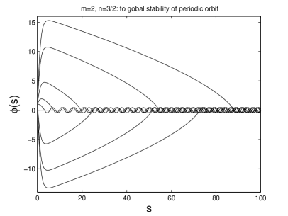
Figure 3. Convergence to the stable periodic solutions of (5.17) for $n=\frac{3}{2}$ for various Cauchy data posed at $s=0$.

Proposition 5.5.

If the periodic solution $\phi_{*}(s)$ of $(\ref{m=2.11})$ persists for all $\frac{3}{2}\leq n_{\rm h}<3$, then it is stable and hyperbolic on this interval.

Proof. Note that, for $n\in(\frac{3}{2},3)$, there exist two unstable constant equilibria of (5.17)

(5.22) $$\phi_{\pm}=\pm\bigl{[}-\frac{1}{\mu(\mu-1)(\mu-2)}\bigr{]}^{\frac{1}{n}}\quad\mbox{for}\,\,\,n\in(\frac{3}{2},3),$$

and we expect a stable periodic motion in between. Consider the eigenvalue problem for the ODE (5.17) linearized about the $T$-periodic solution $\phi_{*}$ by setting $\phi=\phi_{*}+Y$,

$$Y^{\prime\prime\prime}+3(\mu-1)Y^{\prime\prime}+(3\mu^{2}-6\mu+2)Y^{\prime}+\mu(\mu-1)(\mu-2)Y+(1-n)|\phi_{*}|^{-n}Y=\lambda Y.$$

As usual, assuming that $\lambda\in{\mathbb{C}}$, multiplying this by the complex conjugate ${\overline{Y}}$ in $L^{2}(0,T)$, taking the conjugate and multiplying by $Y$, and summing up both yields

(5.23) $$-3(\mu-1)\int|Y^{\prime}|^{2}+\mu(\mu-1)(\mu-2)\int|Y|^{2}+(1-n)\int|\phi_{*}|^{-n}|Y|^{2}=\frac{\lambda+\bar{\lambda}}{2}\int|Y|^{2}.$$

Since all the three terms on the left-hand side of (5.23) are negative for any $\frac{3}{2}<n<3$, the result follows. The case $n=\frac{3}{2}$ is similar since just the second term vanishes. ∎

Thus, by classic branching theory, [42, Ch. 6], stable hyperbolic periodic solutions are locally extensible relative the parameter $n\geq\frac{3}{2}$. In particular, using the hyperbolicity of $\phi_{*}$ for $n=\frac{3}{2}$, we conclude that the periodic solution exists in an interval $n\in[\frac{3}{2},\frac{3}{2}+\delta)$ with some $\delta>0$, and the interval of existence must be open from the right-hand side.

Finally, let us justify the estimate in (5.20). To this end, we multiply (5.17) by $\phi^{\prime}_{*}$ and integrate over $(0,T)$ to get for any $n\in(0,2)$

$$-\int(\phi_{*}^{\prime\prime})^{2}+(3\mu^{2}-6\mu+2)\int(\phi_{*}^{\prime})^{2}=0,$$

so that one needs

$$3\mu^{2}-6\mu+2>0\quad\Longrightarrow\quad\mu=\frac{3}{n}>\mu_{+}=\frac{3}{n_{+}}=\frac{3+\sqrt{3}}{3}.$$

This completes the proof of Theorem 5.4. ∎

On heteroclinic bifurcation. Since the periodic orbit $\phi_{*}(s)$ remains stable and hyperbolic in the whole interval of existence (5.20), the end point $n=n_{\rm h}$ cannot be any kind of subcritical saddle-node bifurcation, at which two branches meet each other. Classic bifurcation and branching theory [32, 42] then suggests that at $n=n_{\rm h}^{-}$ the DS (5.17) undergoes a heteroclinic bifurcation when the period increases without bound (this claim needs further study and a full analytical justification); see standard scenarios in Perko [40, Ch. 4]. Note that, by Proposition 5.5, the heteroclinic orbit occurred remains stable and hyperbolic.

Numerically, $n_{\rm h}$ is given by

(5.24) $$n_{\rm h}=1.7598665026...\,.$$

Figure 4 shows formation of the heteroclinic orbit in both limits: as $n\to n_{\rm h}^{-}$ (a) and $n\to n_{\rm h}^{+}$ (b). This bifurcation exponent $n_{\rm h}$ plays the important role and shows the parameter range of $n$’s, for which many ODE profiles near interfaces are oscillatory except those that approach the interface point $s=-\infty$ the stable manifold of the constant equilibrium (5.22). In the interval (5.21), this manifold of orbits of constant sign is empty, so that all the orbits near $s=-\infty$ are oscillatory and coincide with the periodic one $\phi_{*}(s+s_{0})$, where $s_{0}\in\mathbb{R}$ is a parameter of shifting. Indeed, this also characterizes important oscillatory features of the PDE. Note that some kind of a “heteroclinic bifurcation” phenomenon also exists for the sixth-order ($m=3$) and higher-order TFEs with more difficult mathematics involved; see [18, Sect. 13] and [24, p. 142-147].

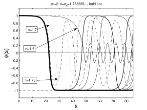
(a) formation as $n\to n_{\rm h}^{-}$

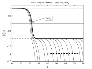
(b) formation as $n\to n_{\rm h}^{+}$

Figure 4. Formation of a heteroclinic orbit as $n\to n_{\rm h}$.

On 1D shooting for $n\in(1,n_{\rm h})$. As a key application of the above oscillation analysis, we have that according to (5.16), for all $n\in(0,n_{\rm h})$, there exists a 1D bundle of oscillatory orbits of changing sign

(5.25) $$F(y)=(1-y)^{\frac{3}{n}}\phi_{*}(\ln(1-y)+s_{0})+...\,,$$

where $s_{0}\in\mathbb{R}$ is an arbitrary parameter of phase shift in the periodic orbit $\phi_{*}(s)$. Recall that, for the ODE (5.14), we need to shoot just a single symmetry condition at the origin,

(5.26) $$F^{\prime}(0)=0\quad(F(0)\not=0),$$

so the 1D bundle (5.25) is well-suited for this. In view of oscillatory character of the behaviour in (5.25), it is not a great deal to prove the existence of such a $s_{0}$ to satisfy (5.26), while uniqueness (as expected) remains open.

Further comments about $n_{\rm h}$. For any $n>n_{\rm h}$, the behaviour in the ODE (5.17) becomes exponentially unstable and we did not observe oscillatory or changing sign patterns. This suggests that precisely above $n=n_{\rm h}$, the ODE (and the corresponding PDE) loses its natural similarities with the linear one for $n=0$ (though a continuous homotopic connection is expected to be still available, i.e., some local properties of solutions dramatically change at $n_{\rm h}$).

Thus, in the range $n\in(\frac{3}{2},3)$, (5.17) possesses the positive constant solution $\phi(s)\equiv\phi_{+}$ given in (5.22). This gives the behaviour (2.35), so that, for such solutions, formally, the FBP and the CP may coincide in the ODE setting. But this is not the case for all the solutions since for $n\in(\frac{3}{2},n_{\rm h})$ there are other oscillatory profiles with a similar (actually, a bit less) regularity at the interfaces, so that the CP demands oscillatory solutions, while the FBP can admit positive solutions; see more details in [17, Sect. 9]. In the parameter range $n\geq n_{\rm h}$, the oscillatory behaviour is no longer generic, so we expect a certain improvement of the positivity preserving properties of the TFE, where the CP and the FBP may coincide; see further discussion in [17, Sect. 9.4].

5.4. The TFE with critical absorption $p=p_{0}$

The formal asymptotics for the TFE (1.5), (1.6) is now calculated similarly using the centre subspace spanned by the eigenfunction (2.29). Of course, we then do not gain any explicit mathematics or symmetric operators as for $n=1$ in the case of the FBP.

The main ideas of the analysis can be extended to the $2m$th-order case, where many aspects of source-type and general solutions of the Cauchy problem for the TFEs remain mathematically open. The oscillatory character of solutions near the interface for $m=3$ was studied in [18, Sect. 13]; see also [24, Sect. 3.7] for further examples for $m\geq 3$ and other oscillatory PDEs.

5.5. Supercritical range $p>p_{0}$

We use the same scaling (3.1) and obtain the exponentially perturbed rescaled PDE (3.2), which suggests that the solutions behave as $t\to\infty$ as the source-type solution with a finite positive mass attained at $\tau=+\infty$ (no proof is still available).

Acknowledgements. The authors would like to thank J.D. Evans for discussions on thin film models with non-conservative aspects, and A. Leger for efficient consulting the authors with numerical methods for higher-order ODEs.

Appendix A The linearised operator is not symmetric when $n\neq 1$

We prove that, in the FBP setting, the linearised operator (2.11) admits a self-adjoint extension only when $n=1$. Without loss of generality we consider the one-dimensional case, and we formulate first the following results we are already familiar with.

Proposition A.1.

The linearised operator $(\ref{2.9})$ in $\mathbb{R}$ is symmetric in some weighted space $L^{2}_{\rho}$ when $n=1$.

Proof. For $N=n=1$, the linearised operator is given by

(A.1) $${\bf A}^{\prime}(f)Y=-(fY^{\prime\prime\prime})^{\prime}-(Yf^{\prime\prime\prime})^{\prime}+\frac{1}{5}\,(Yy)^{\prime}.$$

For this to be symmetric in $L^{2}_{\rho}$ with some weight $\rho\geq 0$, we require that [36, Sect. 1]

(A.2) $${\bf A}^{\prime}(f)Y\equiv\frac{1}{\rho}\,\left[(p_{0}Y^{\prime\prime})^{\prime\prime}-(p_{1}Y^{\prime})^{\prime}+p_{2}Y\right]$$

Expanding the right hand sides of these equations and comparing coefficients yields the following system:

(A.3) $$Y^{\prime\prime\prime\prime} :\,\,\,\mbox{$-f=\frac{p_{0}}{\rho}$},$$

(A.4) $$Y^{\prime\prime\prime} :\,\,\,\mbox{$-f^{\prime}=\frac{2p_{0}^{\prime}}{\rho}$},$$

(A.5) $$Y^{\prime\prime} :\,\,\,\mbox{$0=\frac{p_{0}^{\prime\prime}-p_{1}}{\rho}$},$$

(A.6) $$Y^{\prime} :\,\,\,\mbox{$-f^{\prime\prime\prime}+\frac{1}{5}y=-\frac{p_{1}^{\prime}}{\rho}$},$$

(A.7) $$Y :\,\,\,\mbox{$-f^{\prime\prime\prime\prime}+\frac{1}{5}=\frac{p_{2}}{\rho}$}.$$

We know the exact solution of the ODE for $f$ when $n=1$ (see (1.21)):

(A.8) $$f(y)=\frac{1}{120}\,(a^{2}-y^{2})^{2}\,\,\,\mbox{for}\>y\in(-a,a).$$

Substituting this into equation (A.7) yields $p_{2}=0$. Equation (A.6) yields $p_{1}=C$ where $C$ is a constant. Equations (A.3) and (A.4) yield $p_{0}^{2}=f$ and $\rho=-f^{-1/2}$. Equation (A.5) is thus the consistency condition and is satisfied since it yields $p_{1}=C$ (since $p_{0}^{\prime\prime}=p_{1}=C$). Thus the linearised operator for the thin film equation is symmetric if $n=1$. ∎

Theorem A.2.

For $N=1$ and $n\neq 1$, operator $(\ref{2.9})$ is not symmetric in $L^{2}_{\rho}$ for any weight $\rho>0$.

Proof. The ODE for $f>0$ for any $n>0$ is

(A.9) $$-(f^{n}f^{\prime\prime\prime})^{\prime}+\frac{1}{n+4}\,(fy)^{\prime}=0.$$

The linearised operator (2.11) is given by

(A.10) $${\bf A}^{\prime}(f)Y=-(f^{n}Y^{\prime\prime\prime})^{\prime}-n(f^{n-1}Yf^{\prime\prime\prime})^{\prime}+\frac{1}{n+4}\,(Yy)^{\prime}.$$

For this to be symmetric, we require identity (A.2) to hold. Comparing coefficients yields

(A.11) $$Y^{\prime\prime\prime\prime} :\,\,\,\mbox{$-f^{n}=\frac{p_{0}}{\rho}$},$$

(A.12) $$Y^{\prime\prime\prime} :\,\,\,\mbox{$-nf^{n-1}f^{\prime}=\frac{2p_{0}^{\prime}}{\rho}$},$$

(A.13) $$Y^{\prime\prime} :\,\,\,\mbox{$0=\frac{p_{0}^{\prime\prime}-p_{1}}{\rho}$},$$

(A.14) $$Y^{\prime} :\,\,\,\mbox{$-nf^{n-1}f^{\prime\prime\prime}+\frac{y}{n+4}=-\frac{p_{1}^{\prime}}{\rho}$},$$

(A.15) $$Y :\,\,\,\mbox{$-n(n-1)f^{n-2}f^{\prime\prime\prime}-nf^{n-1}f^{\prime\prime\prime\prime}+\frac{1}{n+4}$}.$$

From this

$$p_{0}^{2}=f^{n},\,\,\,p_{1}=p_{0}^{\prime\prime},\,\,\,\rho=-f^{-n/2},\,\,\,p_{2}=\rho\bigl{[}-n(n-1)f^{n-2}f^{\prime\prime\prime}-nf^{n-1}f^{\prime\prime\prime\prime}+\frac{1}{n+4}\bigr{]},$$

and the consistency condition is

(A.16) $$f^{\frac{n}{2}}(f^{\frac{n}{2}})^{\prime\prime\prime}=-nf^{n-1}f^{\prime\prime\prime}+\frac{1}{n+4}\,y.$$

To see if this coincides with equation (A.9) for some $f$ we use a Taylor expansion of $f(y)$ and check if (A.16) and (A.9) produce the same coefficients for $f$. To do this we set $f(0)=1,\,\,\,f^{\prime}(0)=f^{\prime\prime\prime}(0)=0$ and $f^{\prime\prime}(0)=b\in\mathbb{R}\setminus\{0\}$, differentiate equations (A.16) and (A.9) the required number of times and set $y=0$. The expansions coincide up to the coefficient of $y^{3}$ but the coefficients of $y^{4}$ only coincide if

(A.17) $$b=\pm\frac{\sqrt{-6n(n^{2}+2n-8)(3n-2)}}{3n^{3}+6n^{2}-24n}.$$

Since we require $b\in\mathbb{R}\setminus\{0\}$ we must have $n\in(-4,0)\cup(\frac{2}{3},2)$. This gives us a range of values of $n$, for which the linearised operator may be symmetric. To check whether it is we examine the coefficient of $y^{6}$ for (A.16) and (A.9). If the operator is symmetric, then the same value of $b$ should be obtained as in the coefficients of $y^{4}$ for both equations. For the coefficients of $y^{6}$ to coincide we require

(A.18) $$b=0,\,\,\,\mbox{or}\,\,\,b=\pm\frac{2\sqrt{2}\sqrt{n(9n^{3}-40n^{2}-188n+464)(3n-2)}}{9n^{4}-40n^{3}-188n^{2}+464n}\,,$$

and since we require $b\in\mathbb{R}\setminus\{0\}$ we discard $b=0$. For this $b$ to coincide with (A.17) we require $n=\frac{2}{3}$. This contradicts the fact that we must have $n\in(-4,0)\cup(\frac{2}{3},2)$ for the linearised operator (2.11) to have a chance of being symmetric and admit a suitable (Friedrichs) self-adjoint extension. Hence the linearised operator is not symmetric if $n\neq 1$. ∎

References

- [1] J. Becker and G. Grün, The thin-film equation: recent advances and some new perspectives, J. Phys.: Condens. Matter, 17 (2005), S291–S307.
- [2] D.J. Benney, Long waves on liquid films, J. Math. and Phys., 45 (1966), 150–155.
- [3] F. Bernis and A. Friedman, Higher order nonlinear degenerate parabolic equations, J. Differ. Equat., 83 (1990), 179–206.
- [4] F. Bernis, J. Hulshof, and J.R. King, Dipoles and similarity solutions of the thin film equation in the half-line, Nonlinearity, 13 (2000), 413–439.
- [5] F. Bernis, J. Hulshof, and F. Quirós, The “linear” limit of thin film flows as an obstacle-type free boundary problem, SIAM J. Appl. Math., 61 (2000), 1062–1079.
- [6] F. Bernis and J.B. McLeod, Similarity solutions of a higher order nonlinear diffusion equation, Nonl. Anal., 17 (1991), 1039–1068.
- [7] F. Bernis, L.A. Peletier, and S.M. Williams, Source type solutions of a fourth order nonlinear degenerate parabolic equation, Nonl. Anal., 18 (1992), 217–234.
- [8] A.J. Bernoff and T.P. Witelski, Linear stability of source-type similarity solutions of the thin film equation, Appl. Math. Lett., 15 (2002), 599–606.
- [9] A.L. Bertozzi and M.C. Pugh, Long-wave instabilities and saturation in thin film equations, Comm. Pure Appl. Math., LI (1998), 625–651.
- [10] M.S. Birman and M.Z. Solomjak, Spectral Theory of Self-Adjoint Operators in Hilbert Space, D. Reidel, Dordrecht/Tokyo, 1987.
- [11] M. Bowen, J. Hulshof, and J.R. King, Anomaluous exponents and dipole solutions for the thin film equation, SIAM J. Appl. Math., 62 (2001), 149–179.
- [12] J.A. Carrillo and G. Toscani, Long-time asymptotic behaviour for strong solutions of the thin film equations, Comm. Math. Phys., 225 (2002), 551–571.
- [13] Yu.V. Egorov, V.A. Galaktionov, V.A. Kondratiev, and S.I. Pohozaev, Asymptotic behaviour of global solutions to higher-order semilinear parabolic equations in the supercritical range, Adv. Differ. Equat., 9 (2004), 1009–1038.
- [14] S.D. Eidelman, Parabolic Systems, North-Holland Publ. Comp., Amsterdam/London, 1969.
- [15] C.M. Elliott and H. Garcke, On the Cahn–Hilliard equation with degenerate mobility, SIAM J. Math. Anal., 27 (1996), 404–423.
- [16] C. Elliott and Z. Songmu, On the Cahn-Hilliard equation, Arch. Rat. Mech. Anal., 96 (1986), 339–357.
- [17] J.D. Evans, V.A. Galaktionov, and J.R. King, Source-type solutions of the fourth-order unstable thin film equation, Euro J. Appl. Math., 18 (2007), 273–321.
- [18] J.D. Evans, V.A. Galaktionov, and J.R. King, Unstable sixth-order thin film equation. I. Blow-up similarity solutions; II. Global similarity patterns, Nonlinearity, 20 (2007), 1799–1841, 1843–1881.
- [19] J.D. Evans, V.A. Galaktionov, and J.F. Williams, Blow-up and global asymptotics of the limit unstable Cahn-Hilliard equation, SIAM J. Math. Anal., 38 (2006), 64–102.
- [20] R. Ferreira and F. Bernis, Source-type solutions to thin-film equations in higher dimensions, European J. Appl. Math., 8 (1997), 507–524.
- [21] V.A. Galaktionov, Critical global asymptotics in higher-order semilinear parabolic equations, Int. J. Math. Math. Sci., 60 (2003), 3809–3825.
- [22] V.A. Galaktionov and P.J. Harwin, On evolution completeness of nonlinear eigenfunctions for the porous medium equation in the whole space, Advances Differ. Equat., 10 (2005), 635–674.
- [23] V.A. Galaktionov and S.I. Pohozaev, Blow-up and critical exponents for parabolic equations with non-divergent operators: dual porous medium and thin film operators, J. Evol. Equat, 6 (2006), 45–69.
- [24] V.A. Galaktionov and S.R. Svirshchevskii, Exact Solution and Invariant Subspaces of Nonlinear Partial Differential Equations in Mechanics and Physics, ChapmanHall/CRC, Boca Raton, Florida, 2007.
- [25] V.A. Galaktionov and J.L. Vázquez, A Stability Technique for Evolution Partial Differential Equations. A Dynamical Systems Approach, Progr. in Nonl. Differ. Equat. and their Appl., 56, Birkhäuser Boston, Inc., MA, 2004.
- [26] L. Giacomelli and F. Otto, Groplet spreading: intermediate scaling law by PDE methods, Comm. Pure Appl. Math., 55 (2002), 217–254.
- [27] L.V. Govor, J. Parisi, G.H. Bauer, and G. Reiter, Instability and droplet formation in evaporating thin films of a binary solution, Phys. Rev. E, 71, 051603 (2005).
- [28] H.P. Greenspan, On the motion of a small viscous droplet that wets a surface, J. Fluid Mech., 84 (1978), 125–143.
- [29] G. Grün, Degenerate parabolic equations of fourth order and a plasticity model with non-local hardening, Z. Anal. Anwendungen, 14 (1995), 541–573.
- [30] A.S. Kalashnikov, Some problems of the qualitative theory of second-order nonlinear degenerate parabolic equations, Russian Math. Surveys, 42 (1987), 169–222.
- [31] I.T. Kiguradze and T. Kusano, Periodic solutions of nonautonomous ordinary differential equations of higher order, Differ. Equat., 35 (1999), 71–77.
- [32] M.A. Krasnosel’skii and P.P. Zabreiko, Geometrical Methods of Nonlinear Analysis, Springer-Verlag, Berlin/Tokyo, 1984.
- [33] R.S. Laugesen and M.C. Pugh, Energy levels of steady states for thin-film-type equations, J. Differ. Equat., 182 (2002), 377–415.
- [34] Z. Liu and Y. Mao, Existence theorems for periodic solutions of higher order nonlinear differential equations, J. Math. Anal. Appl., 216 (1997), 481–490.
- [35] V.G. Maz’ja, Sobolev Spaces, Springer-Verlag, Berlin/Tokyo, 1985.
- [36] M.A. Naimark, Linear Differential Operators, Frederick Ungar Publ. Co., New York, 1968.
- [37] A. Oron, Nonlinear dynamics of three-dimensional long-wave Marangoni instability in thin liquid films, Phys. Fluids, 12 (2000), 1633–1645.
- [38] A. Oron, S.H. Davies, and S.G. Bankoff, Long-scale evolution of thin liquids films, Rev. Modern Phys., 69 (1997), 931–980.
- [39] A. Oron and O. Gottlied, Nonlinear dynamics of temporally excited falling liquid films, Phys. Fluids, 14 (2002), 2622–2636.
- [40] L. Perko, Differential Equations and Dynamical Systems, Springer-Verlag, New York, 1991.
- [41] N.F. Smyth and J.M. Hill, High-order nonlinear diffusion, IMA J. Appl. Math., 40 (1988), 73–86.
- [42] M.A. Vainberg and V.A. Trenogin, Theory of Branching of Solutions of Non-Linear Equations, Noordhoff Int. Publ., Leiden, 1974.
- [43] J.R. Ward, Asymptotic conditions for periodic solutions of ordinary differential equations, Proc. Amer. Math. Soc., 81 (1981), 415–420.
- [44] T.P. Witelski, A.J. Bernoff, and A.L. Bertozzi, Blow-up and dissipation in a critical-case unstable thin film equation, Euro J. Appl. Math., 15 (2004), 223–256.