Optical spectroscopy and photometry of SAX J1808.4$-$3658 in outburst

Abstract

We present phase resolved optical spectroscopy and photometry of V4580 Sagittarii, the optical counterpart to the accretion powered millisecond pulsar SAX J1808.4$-$3658, obtained during the 2008 September/October outburst. Doppler tomography of the N iii $\lambda$4640.64 Bowen blend emission line reveals a focused spot of emission at a location consistent with the secondary star. The velocity of this emission occurs at $324\pm 15$ km s^-1; applying a “$K$-correction”, we find the velocity of the secondary star projected onto the line of sight to be $370\pm 40$ km s^-1. Based on existing pulse timing measurements, this constrains the mass ratio of the system to be $0.044^{+0.005}_{-0.004}$, and the mass function for the pulsar to be $0.44^{+0.16}_{-0.13}$ M_☉. Combining this mass function with various inclination estimates from other authors, we find no evidence to suggest that the neutron star in SAX J1808.4$-$3658 is more massive than the canonical value of 1.4 M_☉. Our optical light curves exhibit a possible superhump modulation, expected for a system with such a low mass ratio. The equivalent width of the Ca ii H and K interstellar absorption lines suggest that the distance to the source is $\sim$2.5 kpc. This is consistent with previous distance estimates based on type-I X-ray bursts which assume cosmic abundances of hydrogen, but lower than more recent estimates which assume helium-rich bursts.

1 Introduction

Low mass X-ray binaries (LMXBs) are systems containing a low mass secondary ($M_{2}\lesssim$ 1 M_☉) and a compact primary, either a neutron star (NS) or a black hole (BH). These may be divided into two subclasses based on whether they are persistent or transient sources. The transient systems or X-ray Novae (XRNe) are typically characterised by short periods of heightened luminosity separated by long periods of quiescence. During an XRN outburst the X-ray luminosity increases by 10⁴ – 10⁶, reaching a sizable fraction of the Eddington luminosity. The X-ray outburst is accompanied by an outburst at UV/optical/IR wavelengths dominated by reprocessing of X-rays in the accretion disc (for example, see the review by Charles & Coe, 2006).

Until recently, the vast majority of known XRNe were black hole systems. As a result, systematic comparison between the accretion discs in BH and NS transients was difficult. At the same time, there was little direct evidence for the link between accreting LMXBs and isolated millisecond pulsars that had been anticipated previously (Alpar et al., 1982; Radhakrishnan & Srinivasan, 1984). The discovery of a new class of transient, accretion-powered millisecond X-ray pulsars (AMSPs), simultaneously addressed both of these issues. They provide dramatic confirmation of the link between accreting LMXBs and millisecond pulsars (e.g. Wijnands, 2006): indeed, by combining these observations with measurements of burst oscillations and pulsations from other LMXBs, NS spin periods are now known for 20 LMXBs. The reason why the pulsations are observed in this type of system, with a short orbital period, may be related to the low accretion rate (expected for such short periods), permitting accretion to the polar caps of the NS even in the presence of a relatively weak magnetic field.

SAX J1808.4$-$3658 is the prototypical AMSP. Initially detected by the BeppoSax mission (in ’t Zand et al., 1998), subsequent Rossi X-ray Timing Explorer (RXTE) observations detected coherent millisecond pulsations at a frequency of 401 Hz from a NS in a $\sim$2 hour binary orbit. It was immediately realised that this was the long awaited missing link in the evolution of LMXBs to isolated millisecond pulsars (Wijnands & van der Klis, 1998; Chakrabarty & Morgan, 1998). Subsequent observations revealed the optical counterpart at $R$ $\sim$16.1 mag (Roche et al., 1998). Homer et al. (2001) observed the optical counterpart in the quiescent state and found it to be at $R$ $\simeq 21$ mag. Using recent observations from the Gemini South telescope, Deloye et al. (2008) measure average quiescent magnitudes of $g\simeq 21.7$ mag and $i\simeq 20.6$ mag. The 0.5 – 10 keV X-ray luminosity ($L_{\mathrm{x}}$) of the system is $\sim$$2\times 10^{36}$ erg s^-1 in outburst (in ’t Zand et al., 1998, 2001) and $5\times 10^{31}$ erg s^-1 in quiescence (Campana et al., 2002), for an assumed distance of 2.5 kpc (in ’t Zand et al., 2001). Galloway & Cumming (2006) have calculated that the distance to the source is $\sim$3.5 kpc, assuming that the observed type-I X-ray bursts are helium-rich.

The quiescent optical light curves exhibit sinusoidal variability, the phasing of which indicates that the optical maximum occurs when the secondary is directly behind the pulsar (Homer et al., 2001; Deloye et al., 2008). The observed optical flux is in excess of that expected assuming reprocessing of the measured X-ray flux. It was proposed that the irradiating flux was provided by the spin-down flux from the pulsar (Burderi et al., 2003; Campana et al., 2004), which was irradiating the face of the companion star, hence producing the observed modulation. This effect is similar to that observed in the binary millisecond pulsar PSR B1957+20 (e.g. Reynolds et al., 2007).

To account for their high spin frequencies, the neutron stars in AMSPs are expected to have accreted a few tenths of a solar mass during the lifetime of the binary, and hence should be systematically more massive than the canonical value of $\sim$1.4 M_☉ (Thorsett & Chakrabarty, 1999). Recent quiescent observations (Heinke et al., 2008) have hinted that the NS in SAX J1808.4$-$3658 may be massive ($M_{1}>1.4$ M_☉). Confirmation that the NS is indeed massive could have important implications for efforts to constrain the NS equation of state.

For AMSPs, the orbital period ($P_{\mathrm{orb}}$) and projected semi-major axis of the primary orbit (and hence the projected primary velocity, $K_{1}$) are accurately known from analysis of the X-ray pulse arrival times. Therefore for these systems, only the projected secondary velocity ($K_{2}$) and the binary inclination angle ($i$) are required for the primary mass to be fully constrained. Unfortunately, measurement of the radial velocity of the secondary star in SAX J1808.4$-$3658 in quiescence is not feasible, because of the faintness of the secondary star. However, as Steeghs & Casares (2002) have shown in the case of the LMXB Scorpius X-1, it is possible to identify narrow Bowen blend emission line features (e.g McClintock et al., 1975) formed in the secondary star by fluorescence of UV photons produced in the inner accretion disc, and use these to determine its radial velocity – even when the binary is X-ray bright. This is likely the only means by which we will ever be able to measure the mass of the neutron stars in AMSPs, and confirm their expected massive nature.

In addition, monitoring of these AMSPs provides us with an excellent opportunity to study accretion discs during outburst and to compare the observed structure with quantitative models. For example, in the short period, small mass ratio systems, the disc is expected to be elliptical and precessing (Whitehurst, 1988; Haswell et al., 2001). Doppler tomography of these systems may provide evidence for such an elliptical disc. In addition, strongly X-ray irradiated discs are also susceptible to warping out of the orbital plane (Pringle, 1996; Foulkes, Haswell & Murray, 2006), which should also manifest itself spectroscopically. See Elebert et al. (2008) for the first such study of the AMSP HETE J1900.1$-$2455.

In this paper, we present phased resolved optical spectroscopy and photometry of V4580 Sagittarii, the optical counterpart to the accreting X-ray millisecond pulsar SAX J1808.4$-$3658, obtained during the 2008 outburst (Markwardt & Swank, 2008). The paper is organised as follows: In §2, we describe the spectroscopic and photometric observations. An analysis of these data is presented in §3, in which we show how Doppler tomography of the Bowen blend N iii $\lambda$4640.64 line allows us to measure the mass function of SAX J1808.4$-$3658. Finally, we discuss these results in §4, and present our conclusions in §5.

2 Data

Our data consist of phase resolved spectroscopy and photometry of SAX J1808.4$-$3658, obtained during the 2008 September/October outburst. These observations were motivated by the need to obtain spectroscopy in the region of He ii $\lambda$4686 and the Bowen blend near $\lambda$4640 in an effort to measure the radial velocity of the low mass secondary star ($M_{2}\sim$0.05 M_☉; Bildsten & Chakrabarty, 2001), and hence place constraints on the mass of the pulsar. Although SAX J1808.4$-$3658 is the brightest of all AMSPs in outburst, no optical spectra of the system in this state have been published to date.

Fig. 1 shows the RXTE All-Sky Monitor (ASM) light curve of the outburst, with the dates of our observations marked. The observations at CTIO 1.0-m and 0.9-m telescopes on mjd 54748 were taken at the same time, but have been offset slightly here for clarity.

Figure 1: RXTE ASM light curve, with the dates of our optical observations marked.

2.1 Spectroscopy

A total of 39 optical spectra of SAX J1808.4$-$3658 were acquired with the FOcal Reducer and low dispersion Spectrograph (FORS) 1 and FORS2 spectrographs (Appenzeller et al., 1998), mounted at the Cassegrain foci of the 8.2-m Kueyen (UT2) and Antu (UT1) Very Large Telescopes, respectively, at Cerro Paranal, Chile. The detector on FORS1 consists of a mosaic of two 2000 $\times$ 4000 pixel E2V CCDs (with 15 $\mu$m pixels) while FORS2 has a mosaic of two 2000 $\times$ 4000 pixel MIT CCDs (also with 15 $\mu$m pixels). The output data were binned by a factor of 2 in both spatial and dispersion directions.

On 2008 September 27 ut, 16 spectra were obtained using the 1200B grism on FORS1 with a 0.7 arcsec slit (seeing 0.8 – 1.1 arcsec) and 360 s exposure times, while a further 23 spectra were obtained using the 600B grism on FORS2 with a 1 arcsec slit (seeing 0.6 – 1.0 arcsec) and 240 s exposure times. In all observations, the SAX J1808.4$-$3658 spectrum was on CHIP1 of the FORS1 and FORS2 mosaics. Appropriate bias, flat and comparison HgCd arc lamp frames were also taken.

The data reduction process was identical for both the FORS1 and FORS2 data. The frames were firstly processed using the iraf ccdproc routines to remove instrumental effects. The spectra were then optimally extracted using tasks in the iraf kpnoslit package. Wavelength solutions for FORS1 (FORS2) were found by fitting 2nd order cubic splines to 16 (23) lines in the arc spectra, giving RMS errors of $\sim$0.016 (0.036) Å, and these solutions were then applied to the science frames. The resulting wavelength range was $\lambda\lambda$3620 – 5050 (3330 – 6350), with a dispersion of $\sim$0.70 (1.49) Å pixel^-1 and a resolution (measured from arc lamp lines) of $\sim$1.6 – 1.9 (4.3 – 4.8) Å.

Because only one arc lamp exposure was taken during the daytime for each dataset, night skylines were examined in the SAX J1808.4$-$3658 frames to correct for instrumental flexure. For both the FORS1 and FORS2 datasets, a similar correction routine was employed. Firstly, the relative offsets between the wavelength scales for each of the individual spectra were found by cross-correlating each of the sky spectra against the last spectrum in the set (preliminary template), using the rvsao package in iraf (Kurtz & Mink, 1998). These offsets were used to shift each of the individual spectra onto the wavelength scale of the preliminary template, and the resulting spectra were averaged to produce a master sky template. The positions of the strongest skylines were examined in this master template, in order to compute an average absolute shift. The master template was shifted by this amount, so that all lines appeared at their correct wavelengths, and the final shifts required for each spectrum were found by cross-correlating the spectra against the shifted master template. These shifts were then applied to both the data and error bands of each spectrum. The required shifts for the FORS1 data were within $\pm$0.07 Å for each spectrum. For the FORS2 data, the required shifts were larger, $\sim$0.5 – 0.7 Å. The reduction procedure was repeated and confirmed using the FORS pipeline software

The data were then imported into the molly spectral analysis package, where they were shifted to the heliocentric rest frame, and re-binned onto a common velocity scale of 49 km s^-1 pixel^-1 for the FORS1 data and 95 km s^-1 pixel^-1 for the FORS2 data. The continuum was removed by dividing by a cubic spline function (after masking the emission and absorption features) and subtracting unity. The normalized averaged FORS1 and FORS2 spectra are shown in Fig. 2. The orbital phase was determined using the X-ray ephemeris of Jain, Dutta & Paul (2008). We transformed the $T_{0}$ (epoch when the pulsar is at the ascending node) of the ephemeris from tdb to ut, using the xTime tool, assuming that for the purposes of this work, tdb is equal to tt and also that the heliocentre and barycentre are identical. We also shifted $T_{0}$ forward by one quarter of an orbital period, so that phase zero represents superior conjunction of the pulsar i.e. when the pulsar is at 90$\degr$ orbital longitude from the ascending node. The ephemeris we used was therefore $T_{0}=2450915.398669\ \textsc{hjd}\ \textsc{ut}$ and $P_{\mathrm{orb}}=0.0839022785\ \mathrm{d}$.

Figure 2: FORS1 (bottom), FORS2 (middle) and combined (top) averaged normalized spectra obtained on 2008 September 27. The spectra have been shifted to the rest frame of the system, using the systemic velocity of $-83$ km s^-1 found in §3, and offset vertically for clarity.

Because the primary lines of interest were the Bowen blend and He ii $\lambda$4686, the data near these wavelengths were normalized separately, to ensure optimum continuum removal.

2.2 Photometry

In an effort to constrain the binary inclination angle via fitting the light curve with a physical model of the light sources (e.g. Deloye et al., 2008), we obtained phase resolved photometry of SAX J1808.4$-$3658 from several telescopes during the 2008 September/October outburst. On 2008 October 1 ut, we obtained 20 Gunn/SDSS $i$-band images using the 2-m Faulkes South Telescope, at Siding Spring Observatory, Australia. The EA02 camera was used, which has 2048 $\times$ 2048 pixels binned 2 $\times$ 2 into effectively 1024 $\times$ 1024 pixels, each of which is 0.278 arcsec pixel^-1; the total field of view is 4.7 $\times$ 4.7 arcmin.

On 2008 October 7/8 ut we obtained 40 Gunn $r$-band images from the 1-m SMARTS/Yale Telescope, operated by the SMARTS consortium, at Cerro Tololo Inter-American Observatory (CTIO), Chile. A further 31 Gunn $r$-band images were obtained from the same telescope on 2008 October 8/9 ut. The CCD system used for the observations was built by NOAO and Fermi National Accelerator Laboratory as part of the development of the Dark Energy Camera project (see www.darkenergysurvey.org and DePoy et al., 2008, for more details). The detector in the system is a thick, fully depleted $2048\times 2048$ pixel CCD with 15 $\mu$m pixels, which corresponded to approximately 0.3 arcsec pixel^-1 on the sky. The exposure time for all observations was 300s. The raw images were bias corrected, trimmed, and flat-fielded using the ccdproc routines in iraf.

On 2008 October 9 ut we obtained 9 Bessel $V$-band images using the 0.9-m SMARTS Telescope, also at CTIO. On October 12, we acquired 8 Bessel $R$-band images. The SITe CCD has 2048 $\times$ 2046 pixels, with 0.4 arcsec pixel^-1. As the CCD was read out using 4 amplifiers, the frames were bias corrected and flat-fielded using tasks in the iraf quadproc package.

Photometry was performed using the daophot (Stetson, 1987) point spread function fitting package in iraf. The magnitude of SAX J1808.4$-$3658 was found by comparison with the three stars listed in table 1 of Greenhill, Giles & Coutures (2006). For the $i$- and $r$-band frames, we firstly transformed the $R$-band magnitudes to $r$-band using equation 4 of Jordi, Grebel & Ammon (2006) (for $V-R\leq 0.93$) and $I$-band to $i$-band using equation 8 of Jordi et al. (2006). Fig. 3 shows three light curves, phased using the ephemeris defined in §2.1, and plotted twice for clarity. Two of our data sets were obtained contemporaneously, and these are plotted in Fig. 4.

Figure 3: Light curves of SAX J1808.4$-$3658, folded on the ephemeris defined in §2.1, and plotted twice for clarity. (a) $i$-band data obtained with the Faulkes South telescope on 2008 October 1 ut. (b) $r$-band data obtained with the CTIO 1-m telescope on 2008 October 7/8 ut. (c) Bessel $R$-band data obtained with the 0.9-m CTIO telescope on 2008 October 12 ut. All three light curves have the same magnitude scale.

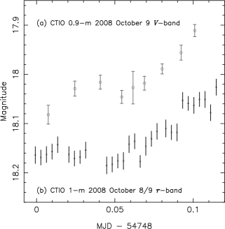
Figure 4: Light curves of SAX J1808.4$-$3658. (a) $V$-band data obtained with the 0.9-m CTIO telescope on 2008 October 9 ut (circles). (b) $r$-band data obtained with the CTIO 1-m telescope on 2008 October 8/9 ut (squares). Note that the $r$-band light curve has been shifted down by 0.1 mag for clarity.

3 Results

3.1 Photometry

The main purpose of our photometry was to identify a modulation that could be used to constrain the binary inclination angle, by fitting the data using, for example, the elc code of Orosz & Hauschildt (2000).

Out first light curve was obtained by Faulkes South just as SAX J1808.4$-$3658 was beginning to decline from the outburst. Although the minimum occurs near phase zero, the overall variation is more reminiscent of a superhump modulation (see e.g. Patterson et al., 2005), or indeed a pre-eclipse hump from the hotspot (see e.g. Grauer et al., 1994), than a modulation due to the heated secondary star. Our second light curve was obtained when SAX J1808.4$-$3658 had declined further from outburst maximum: this light curve exhibits a modulation closest to what might expected from a heated secondary (see Fig. 3), although a superhump modulation cannot be ruled out. If this modulation is due to a heated secondary, a reasonable fit to the light curve (using elc) can be achieved for any of the range of inclination angles found by Deloye et al. (2008). Our remaining light curves do not exhibit any obvious orbital modulation. Hence we conclude that these data cannot be used to place reliable constraints on the orbital inclination. Our light curves cover just over one orbital period each, so it also possible that the observed modulations are due to fluctuations in the mass accretion rate.

Jordi et al. (2006) have very little data for $V-R\simeq 0$, but assuming that their transformations are valid in this regime, we transformed the 2008 October 7/8 ut CTIO 1-m $r$-band magnitudes to Johnson-Cousins $R$-band by using the simultaneous $V$-band data, to give $V-R=0.12\pm 0.04$ mag. This is consistent with the measurements in fig. 2 of Greenhill et al. (2006). De-reddening the $R$- and $V$-band magnitudes using our measured $A_{\mathrm{V}}=0.8\pm 0.3$ (see §3.2) yields $(V-R)_{0}=-0.08\pm 0.09$ mag on this night.

3.2 Spectroscopy

Our spectra (Fig. 2) are dominated by broad Balmer absorption lines, with interstellar Ca ii H and K and Na D absorption lines, and emission lines from the Bowen blend near $\lambda$4640 and from He ii $\lambda$4686. The diffuse interstellar band (DIB) at $\lambda$5780 is also present. The main characteristics of these features are summarised in Table 1.

The Balmer lines from SAX J1808.4$-$3658 itself extend to very high velocities, implying that they are produced in the optically thick accretion disc. There is some infilling of these lines by red-shifted emission features, most obviously in the H$\beta$ absorption line. The H$\gamma$ absorption line appears unusually narrow, compared with the other Balmer lines. It also appears to be blue-shifted relative to its rest wavelength, while the other Balmer lines seem to be relatively symmetrical about the rest wavelength, apart from the red-shifted emission. This may be due to higher levels of red-shifted emission in the H$\gamma$ line, although why this should be is unclear. This effect is present in both the FORS1 and FORS2 data, and so would not appear to be a wavelength calibration issue.

Table 1: Equivalent width and full-width half-maximum for the strongest features in the SAX J1808.4$-$3658 average spectrum.

	EW	______ FWHM ______
	(Å)	(Å)	(km s-1)
He ii $\lambda$4686	$-0.85\pm 0.16$	$23\pm 6$	$1500\pm 400$
Bowen blend	$-0.35\pm 0.16$	…….	……..
H$\beta$	$5.0\pm 0.4$	$70\pm 6$	$4300\pm 400$
H$\gamma$	$2.8\pm 0.3$	$37\pm 3$	$2600\pm 200$
H$\delta$	$4.5\pm 0.3$	$48\pm 3$	$3500\pm 200$
H$\epsilon$	$2.5\pm 0.2$	$32\pm 3$	$2400\pm 200$
H$\zeta$	$2.3\pm 0.2$	$29\pm 3$	$2200\pm 200$
H$\eta$	$1.2\pm 0.2$	$22\pm 4$	$1700\pm 300$
He i $\lambda$4472	$1.0\pm 0.3$	$40\pm 15$	$2700\pm 1000$
Interstellar features
Ca ii K $\lambda$3933.67	$0.77\pm 0.07$	……..	……..
Ca ii H $\lambda$3968.47	$0.56\pm 0.08$	……..	……..
Na D1 $\lambda$5889.95	$0.97\pm 0.12$	……..	……..
Na D2 $\lambda$5895.92	$0.68\pm 0.12$	……..	……..
DIB $\lambda$5870	$0.14\pm 0.04$	……..	……..

3.2.1 Extinction and distance

$E(B-V)$ is a function of the equivalent width (EW) of the DIB at $\lambda$5870. Using four of the stars in table 1 of Jenniskens & Desert (1994), $EW(5780)/E(B-V)=0.52\pm 0.11$. For SAX J1808.4$-$3658 $EW(5780)=0.14\pm 0.04$, therefore we find $E(B-V)=0.27\pm 0.11$. This correlation is also shown by Webster (1993) (fig. 5), and the point (0.27, 0.14) lies close to a best-fitting line through the low $E(B-V)$ ($<0.5$) points. The errors (here and in the remainder of the paper) represent the 1$\sigma$ uncertainties (or 68.3% confidence intervals for non-normal distributions), calculated using Monte Carlo simulations assuming Gaussian statistics.

Fitting the X-ray spectra reveals that the hydrogen column density to the source ($N_{\mathrm{H}}$) is equal to $(1.3\pm 0.1)\times 10^{21}$ cm^-2 (Campana, Stella & Kennea, 2008). Taking $N_{\mathrm{H}}/E(B-V)=5.0\times 10^{21}$ cm^-2 mag^-1 (Savage & Mathis, 1979, and references therein), with a 1$\sigma$ error of 30% (Bohlin et al., 1978), this implies $E(B-V)=0.26^{+0.11}_{-0.06}$, consistent with the value found using the DIB.

Munari & Zwitter (1997) examine the relationship between the EW of the Na D₁ line and $E(B-V)$. The values of $E(B-V)$ we calculate above are only consistent with their analysis if the Na D absorption lines towards SAX J1808.4$-$3658 have multiple components. Our spectral resolution is too low to determine if this is the case. The ratio of Na D₁ to Na D₂ is $\sim$1.4, which is also consistent with a relatively low $E(B-V)$.

Taking $E(B-V)=0.27\pm 0.11$, $A_{\mathrm{V}}=0.8\pm 0.3$. This is consistent with the value found by Wang et al. (2001).

Megier et al. (2005) established relationships between the EW of the Ca ii K and H interstellar absorption lines and the distance to the source. Such a relationship suggests that Ca ii is homogeneously distributed throughout the interstellar medium (Galazutdinov, 2005). These relationships suggest a distance to SAXJ1808.4$-$3658 of $2250\pm 230$ pc based on the Ca ii K line and $2700\pm 400$ pc based on the Ca ii H line. The combined distance estimate is $2500\pm 400$ pc.

3.2.2 Projected velocity of the donor star

As discussed in §1, for systems with low luminosity companions like SAX J1808.4$-$3658, the only way to determine the projected velocity of the secondary star is by observing the radial velocity shifts of the Bowen emission lines near $\lambda$4640. The primary features contained in the Bowen blend are N iii emission lines at $\lambda\lambda$4634.13, 4640.64, 4641.85 and 4641.96, and C iii emission lines at $\lambda\lambda$4647.4 and 4650.1. In the majority of systems so far observed, the N iii $\lambda$4640.64 line is the strongest of these (Cornelisse et al., 2008).

In some systems, the velocity shift of these individual lines can be observed as S-waves in a trailed spectrogram (e.g Steeghs & Casares, 2002; Casares et al., 2006). In other cases, the S/N and resolution of the observations are such that the S-waves are not obvious, but the presence of velocity shifts is revealed by performing Doppler tomography (Marsh & Horne, 1988; Marsh, 2001) of the spectra (e.g. Casares et al., 2003). Casares et al. (2004) report on a successful implementation of this technique for the AMSP XTE J1814$-$338, which revealed the velocity of the donor star emission to be 345 km s^-1. Elebert et al. (2008) attempted this for another AMSP, HETE J1900.1$-$2455, but the S/N of their data was insufficient to provide a reliable measurement.

Before attempting to detect the secondary star in either the trailed spectra or Doppler tomograms, we firstly used the existing information about the system to determine the expected range of projected secondary velocities. Analysis of the pulse arrival times (Chakrabarty & Morgan, 1998; Jain et al., 2008) provides us with very accurate values of $P_{\mathrm{orb}}$ ($7249.156862\pm 0.000005$ s) and $a_{1}\sin{i}$ ($62.809\pm 0.001$ light-ms), which combine to give the primary velocity, $K_{1}=2\pi a_{1}\sin{i}/P_{\mathrm{orb}}=16.32056\pm 0.00026$ km s^-1. Since the primary is a NS, we assume an extreme primary mass range of 1.4 – 3.0 M_☉, and that $i$ lies between 5$\degr$ and 90$\degr$.

The mass function equation relates the mass of the primary to these observable quantities.

$$f(M)=\frac{M_{1}\sin^{3}{i}}{(1+q)^{2}}=\frac{K_{2}^{3}P_{\mathrm{orb}}}{2\pi G}=\frac{K_{1}^{3}P_{\mathrm{orb}}}{2\pi Gq^{3}}$$ (1)

where $q$ is the binary mass ratio ($\equiv M_{2}/M_{1}=K_{1}/K_{2}$) By solving Equation 1 for the cubic in $q$, we calculated $K_{2}$ for a range of $i$ and $M_{1}$, and plot $K_{2}$ vs. $M_{1}$ for several values of $i$ in Fig. 5.

Figure 5: $K_{2}$ vs. $M_{1}$ for inclination angles of 5$\degr$, 30$\degr$, 60$\degr$ and 90$\degr$.

This plot shows that, for $M_{1}<3$ M_☉ and all possible inclination angles, $K_{2}<700$ km s^-1. Because the ephemeris is known so accurately from the pulse timing analysis, emission from the secondary should appear very close to the positive $V_{\mathrm{y}}$ axis, and at a velocity less than 700 km s^-1, in our Doppler tomograms.

In order to perform Doppler tomography, a parameter which must be known is the systemic velocity ($\gamma$), as this determines the offset of any underlying S-wave from the rest wavelength. Ideally, this should be obtained using radial velocity studies of the secondary star: this is impossible here however. Instead, we determined a value for $\gamma$ by fitting a Gaussian to the He ii $\lambda$4686 line, after masking the line core. If the flux in the wings of this emission line originates in the inner accretion disc, then a fit to the wings of this line should provide a reasonable estimate of $\gamma$, where the flux is less contaminated by irregularities in the outer disc such as the gas stream/accretion disc impact region (although see the discussion by Marsh, 1998). For the NS LMXB Cygnus X-2 (Elebert et al., 2009), and BH LMXB XTE J1118+480 (Elebert et al., in preparation.), the wings of this line, averaged over an entire orbital period, provide values for $\gamma$ consistent (within the errors) with those found by analysis of the secondary star absorption line spectra.

For the FORS1 data, the best fit gives $\gamma=-77\pm 14$ km s^-1, while for the FORS2 data, we get a best fit $\gamma$ of $-77\pm 16$ km s^-1. Unfortunately, the Balmer absorption lines were too broad to confirm these values.

Our Doppler tomograms were constructed using the maximum entropy method (MEM), as implemented in doppler. An initial value for $\gamma$ of $-77$ km s^-1 was chosen for both the FORS1 and FORS2 tomograms. Since the N iii $\lambda$4640.64 emission line is generally the strongest in the Bowen blend, we first attempted to make Doppler tomograms of this line. The tomograms were iterated to minimize the reduced $\chi^{2}$ ($\chi^{2}_{\nu}$) between the data and tomogram, while maintaining a smooth image. Both FORS1 and FORS2 tomograms showed clear emission near the positive $V_{\mathrm{y}}$ axis, where emission from the secondary is expected, and in both cases this emission was at a value of $\sim$300 km s^-1. Using the 3$\sigma$ range in systemic velocity, Doppler tomograms of the other Bowen blend lines did not show any emission from near the $V_{\mathrm{y}}$ axis, nor any focused spots of emission at any phase or velocity.

We then combined both datasets and a Gaussian fit to the wings of the averaged He ii $\lambda$4686 line gave a value for $\gamma$ of $-83\pm 12$ km s^-1. As an independent check on the value of $\gamma$, Doppler tomograms of the N iii $\lambda$4640.64 emission line were created for a range of $\gamma$ values, and the spot characteristics (peak and FWHM) were measured in each tomogram by fitting with a point spread function. When the ratio of the peak to FWHM was plotted against $\gamma$, a maximum was observed at $\gamma=-55\pm 20$ km s^-1, which we regard as consistent with our estimate from the He ii $\lambda$4686 line. We note that the spot of emission is closest to the $V_{\mathrm{y}}$ axis near $\gamma=-80$ km s^-1, and so we adopt a value for $\gamma$ of $-83\pm 12$ km s^-1, as determined from the He ii $\lambda$4686 line fitting.

We created several Doppler tomograms from these data using $\gamma=-83$ km s^-1, with different velocity binnings, phase binnings and filtering. In all cases, we observed a bright spot of emission on the positive $V_{\mathrm{y}}$ axis near 300 km s^-1. Fig. 6 shows the Doppler tomogram for the case where we re-binnned all the data at 49 km s^-1, and into 20 phase bins. The centroid of the spot of emission is at a velocity of $K_{\mathrm{em}}=324\pm 8$ km s^-1. For Doppler tomograms within the 1$\sigma$ range of $\gamma$ values, the spot remained focused and close to the same value of $324\pm 8$ km s^-1. We estimate that the effect of the spot location dependency on $\gamma$ increases the 1$\sigma$ error on $K_{\mathrm{em}}$ to 15 km s^-1. Again, none of the other Bowen blend lines showed any focused spots of emission in their tomograms. The spectra extracted using the FORS pipeline software, and processed in an identical manner, yielded identical results, within the uncertainties.

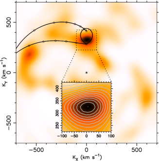
Figure 6: Doppler tomogram of the N iii $\lambda$4640.64 emission line using the combined FORS1 and FORS2 data. The Roche lobe of the secondary for $K_{2}=370$ km s^-1 and $q=0.044$, the gas stream from the inner Lagrangian point and the velocity of the disc along the gas stream are overplotted.

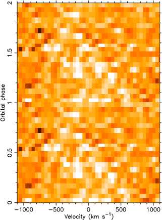
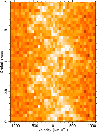
Figure 7: Trailed spectrum of the N iii $\lambda$4640.64 emission line using the combined FORS1 and FORS2 data, in 20 phase bins (top panel) and trailed spectrum computed from the Doppler tomogram in Fig. 6 (bottom panel).

3.2.3 The $K$-correction

$K_{\mathrm{em}}$ is the velocity of the inner hemisphere of the secondary, and a correction must be applied to obtain the velocity of the centre of mass of the secondary – the $K$-correction. This correction is the ratio of the velocity of the Bowen emitting region to the velocity of the centre of mass of the secondary, and depends on how the secondary is irradiated by the central source. By simulating the irradiation of the secondary, Muñoz-Darias, Casares & Martínez-Pais (2005) computed $K$-correction values for a range of mass ratios, inclinations and disc flaring angles (the opening angle of the disc rim above the plane, $\alpha$). They fit their simulation results with 4th order polynomials in $q$, and present the coefficients for various values of $\alpha$, and for $i=40\degr$ and $90\degr$.

Since $K_{1}$ is known to high accuracy from the pulse timing analysis, we estimated a value of $q$ as the ratio $K_{1}$ to $K_{\mathrm{em}}$, calculated a $K$-correction based on this, then iterated until a value of $K_{2}$ was converged upon. We used the polynomial coefficients computed for $i=40\degr$ (although we found very little difference for the $i=90\degr$ coefficients), and calculated the $K$-correction for a range of values of $\alpha$. The maximum value of $\alpha$, for which irradiation of the secondary would still occur, was also calculated for the different values of $q$. Based on this, $\alpha$ must be less than $\sim$9$\degr$, since, regardless of the value of $q$, any value of $\alpha$ greater than 9$\degr$ would cause the secondary to be totally shielded from the primary/inner disc by the disc. Within the 1$\sigma$ range of values for $K_{\mathrm{em}}$ (309 – 339 km s^-1) and for all values of $\alpha\leq 9\degr$, we find $K_{2}=370\pm 40$ km s^-1. Therefore, our estimate for $K_{2}$ is quite conservative, as it takes the full range of possible values of $\alpha$ into account, since we have no way of determining $\alpha$. Combining our measurement of $K_{2}=370\pm 40$ km s^-1 with the existing parameters and Equation 1, we find $q=0.044^{+0.005}_{-0.004}$, $f(M)=0.44^{+0.16}_{-0.13}$ M_☉ and $M_{1}\sin^{3}{i}=0.48^{+0.17}_{-0.14}$ M_☉.

3.2.4 He II $\lambda$4686 Doppler tomography

Using $\gamma=-83$ km s^-1 we created a Doppler tomogram of the He ii $\lambda$4686 emission line. The input data we used was similar to that used for the N iii $\lambda$4640.64 line – velocity binned to 49 km s^-1 pixel^-1, in 20 phase bins. Fig. 8 shows the Doppler tomogram of the He ii $\lambda$4686 line, with the Roche lobe of the secondary, gas stream velocity and velocity of the stream along the accretion plotted for $K_{2}=370$ km s^-1 and $q=0.044$. The main feature of the tomogram is a bright spot of emission, along the gas stream trajectory. Whether this coincides with the location of the gas stream/accretion disc impact point is unclear. There is also a roughly circular pattern, due to the accretion disc, although this is much more apparent in tomograms where the $\chi^{2}_{\nu}$ has not been decreased to as low a value. Fig. 9 shows the trailed spectrogram used to produce this Doppler tomogram, as well as the spectrogram computed from the Doppler tomogram.

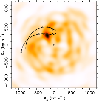
Figure 8: Doppler tomogram of the combined FORS1 and FORS2 data for the He ii $\lambda$4686 emission line. The Roche lobe of the secondary for $K_{2}=370$ km s^-1 and $q=0.044$, gas stream from the inner Lagrangian point and velocity of the disc along the gas stream are overplotted.

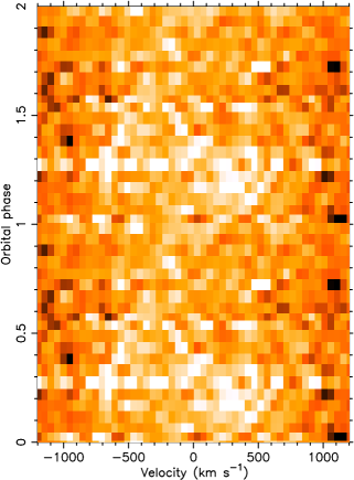
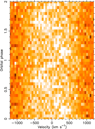
Figure 9: Trailed spectrum of the He ii $\lambda$4686 emission line using the combined FORS1 and FORS2 data, in 20 phase bins (top panel) and trailed spectrum computed from the Doppler tomogram in Fig. 8 (bottom panel).

4 Discussion

4.1 The mass of the pulsar

Fig. 10 shows a plot of $K_{2}$ vs. $i$ for primary masses of 1.4, 1.8, 2.2, 2.6 and 3.0 M_☉. Based on our estimates for the system parameters, we calculate that for a primary mass between 1.4 and 3.0 M_☉, the inclination angle must lie between 33$\degr$ and 44$\degr$ for $K_{2}=370$ km s^-1 and between 29$\degr$ and 51$\degr$ for the 1$\sigma$ range of values in $K_{2}$. For pulsar masses of 1.4 – 3.0 M_☉, our value of $q$ leads to companion masses of $\sim$0.06 – 0.13 M_☉.

Figure 10: $K_{2}$ vs. $i$ for primary masses of 1.4, 1.8, 2.2, 2.6 and 3.0 M_☉. The dashed lines mark the allowed range of inclination angles if $K_{2}=370$ km s^-1, and the dotted lines show the range of angles at the 1$\sigma$ limits on $K_{2}$.

Our data provide us with a value for $M_{1}\sin^{3}{i}=0.48^{+0.17}_{-0.14}$ M_☉. In order to determine the primary mass, the only remaining parameter that must be found is the inclination angle. There have been several attempts to constrain the orbital inclination of SAX J1808.4$-$3658. Deloye et al. (2008) have published Gemini SDSS $i$- and $g$-band light curves of SAX J1808.4$-$3658 in quiescence, and find that the 2$\sigma$ range of values for the inclination is 32 – 74$\degr$, irrespective of the primary mass. Hence, for an inclination of $53\degr\pm 11\degr$ (1$\sigma$), we derive a pulsar mass of $1.0^{+0.8}_{-0.4}$ M_☉.

X-ray measurements taken during the 2008 outburst also help to constrain the inclination angle. For example, using observations from Suzaku, Cackett et al. (2009) fit the relativistically broadened Fe K line, and found a value of $i=55^{+8}_{-4}$ degrees (90% confidence). Combining this estimate with our measurements leads to a primary mass of $0.9\pm 0.3$ M_☉ (1$\sigma$). By analysing RXTE data from the 2002 outburst, Ibragimov & Poutanen (2009) find a value of $i=60\pm 5\degr$, consistent with the results of Cackett et al. (2009) and Deloye et al. (2008), within the uncertainties.

Although all of these estimates are somewhat model dependent, it is clear that, when combined with our results, they do not support a heavy NS in SAX J1808.4$-$3658. This would suggest that the NS in SAX J1808.4$-$3658 has not accreted a significant amount of material, implying that the mass transfer has been non-conservative over the lifetime of the system.

4.2 Accretion disc

Our spectra show broad Balmer absorption lines, with some in-filling of the cores on the red sides of the lines. These absorption lines originate in the optically thick accretion disc. The spectra show similarities to the spectra of KS Ursae Majoris (Zhao et al., 2006), an SU UMa type (i.e. exhibits superhumps during superoutbursts) cataclysmic variable system. In particular, the Balmer absorption lines show some infilling in both cases, with this effect more pronounced at longer wavelengths. The offset emission we observe may have an origin in an eccentric precessing accretion disc, as was also observed in the spectra of the LMXB XTE J1118+480 (Torres et al., 2002). Helium absorption is at most very weak, which suggests that the accretion disc is dominated by hydrogen.

The optical photometry reveals a modulation which may be due to the phase dependent visibility of the irradiated face of the secondary star, similar to the situation in quiescence (e.g. Deloye et al., 2008). However, it is more likely that this modulation is due to a superhumping accretion disc, or simply due to variations in the mass transfer rate onto the NS. Superhumps are periodic optical modulations, originally seen during superoutbursts of SU UMa dwarf novae (DNe), but also seen in some LMXBs in outburst (Haswell et al., 2001, and references therein). The superhump period ($P_{\mathrm{sh}}$) is typically a few percent longer than $P_{\mathrm{orb}}$, although we have insufficient data here to determine if this is the case for SAX J1808.4$-$3658.

The Faulkes $i$-band light curve shown in Fig. 3(a) is more like a sawtooth pattern, rather than the sinusoid-like variation expected if the modulation was due to the secondary star. Although the minimum of this light curve occurs near phase zero, the maximum brightness is at phase 0.7 – 0.8, rather than phase 0.5. The CTIO 1-m $r$-band light curve in Fig. 3(b) is more sinusoidal, but the amplitude of the modulation is a factor of $\sim$2 lower than in the $i$-band light curve. The CTIO 0.9-m $R$-band light curve shows no discernible modulation. Another AMSP, HETE J1900.1$-$2455 exhibits superhumps (Elebert et al., 2008), and in this case the amplitude of the superhumps varied by a factor of $\sim$3 over 11 days, without any significant change in the X-ray brightness. For $L_{\mathrm{x}}$ $\sim$10³⁶ erg s^-1 the accretion disc is also likely to exhibit warping caused by the irradiation. Whether or not this is the case for SAX J1808.4$-$3658 is unclear, but the combination of apsidal and warped precession may explain why some of our light curves appear to exhibit periodic variations, and others do not. We also note that most of our light curves cover a single orbital period only, and hence we cannot exclude the possibility that purely random variations in the mass transfer rate could give rise to the apparent superhump variability discussed here.

5 Conclusions

We have presented Doppler tomography of the N iii $\lambda$4640.64 emission line for SAX J1808.4$-$3658, from which we find the velocity of the emission to be at $324\pm 15$ km s^-1. Applying the $K$-correction, we find the projected velocity of the centre of mass of the secondary star to be $370\pm 40$ km s^-1. Combining this with existing parameters, we constrain the mass ratio to be $0.044^{+0.005}_{-0.004}$, and the mass function of the pulsar to be $0.44^{+0.16}_{-0.13}$ M_☉. Hence, the mass of the pulsar is $0.48^{+0.17}_{-0.14}/\sin^{3}{i}$ M_☉.

Using various estimates of the binary inclination angle we find no evidence to suggest that the neutron star in SAX J1808.4$-$3658 is more massive than the canonical value of 1.4 M_☉, despite the fact that AMSPs are expected to have accreted a significant fraction of a solar mass in order to attain such rapid spin frequencies.

An important next step in determining the mass of the neutron star in SAX J1808.4$-$3658 is to confirm the orbital inclination estimate from the Fe K line fitting (Cackett et al., 2009). The outburst optical light curves appear to be dominated by the disc and not, for example, by an X-ray heated secondary that could be modelled to infer the inclination. In quiescence, however, a modulation due to a heated secondary is clearly visible (e.g. Deloye et al., 2008), and more detailed multicolour modelling here is probably the best route to confirming the inclination.

Determining the masses of the neutron star in AMSPs is challenging for a number of reasons. However, because of the ability to accurately measure the orbital period and projected velocity of the neutron star using the X-ray pulses, these AMSPs remain the most promising systems for determining neutron star masses, helping to constrain the equation of state which describes matter in these neturon stars.

References

- Alpar et al. (1982) Alpar M. A., Cheng A. F., Ruderman M. A., Shaham J., 1982, Nature, 300, 728
- Appenzeller et al. (1998) Appenzeller I. et al., 1998, The Messenger, 94, 1
- Bildsten & Chakrabarty (2001) Bildsten L., Chakrabarty D., 2001, ApJ, 557, 292
- Bohlin et al. (1978) Bohlin R. C., Savage B. D., Drake J. F., 1978, ApJ, 224, 132
- Burderi et al. (2003) Burderi L., Di Salvo T., D’Antona F., Robba N. R., Testa V., 2003, A&A, 404, L43
- Cackett et al. (2009) Cackett E. M., Altamirano D., Patruno A., Miller J. M., Reynolds M. T., Linares M., Wijnands R., 2009, ApJ submitted
- Campana et al. (2004) Campana S. et al., 2004, ApJ, 614, L49
- Campana et al. (2002) Campana S. et al., 2002, ApJ, 575, L15
- Campana et al. (2008) Campana S., Stella L., Kennea J. A., 2008, ApJ, 684, L99
- Casares et al. (2006) Casares J., Cornelisse R., Steeghs D., Charles P. A., Hynes R. I., O’Brien K., Strohmayer T. E., 2006, MNRAS, 373, 1235
- Casares et al. (2004) Casares J., Steeghs D., Hynes R. I., Charles P. A., Cornelisse R., O’Brien K., 2004, in Tovmassian G., Sion E., eds, Revista Mexicana de Astronomia y Astrofisica Conference Series Vol. 20, Bowen Fluorescence from Companion Stars in X-ray Binaries. pp 21–22
- Casares et al. (2003) Casares J., Steeghs D., Hynes R. I., Charles P. A., O’Brien K., 2003, ApJ, 590, 1041
- Chakrabarty & Morgan (1998) Chakrabarty D., Morgan E. H., 1998, Nature, 394, 346
- Charles & Coe (2006) Charles P. A., Coe M. J., 2006, Optical, ultraviolet and infrared observations of X-ray binaries. Compact stellar X-ray sources, pp 215–265
- Cornelisse et al. (2008) Cornelisse R., Casares J., Muñoz-Darias T., Steeghs D., Charles P., Hynes R., O’Brien K., Barnes A., 2008, in American Institute of Physics Conference Series Vol. 1010, An Overview of the Bowen Survey: Detecting Donor Star Signatures in Low Mass X-ray Binaries. pp 148–152
- Deloye et al. (2008) Deloye C. J., Heinke C. O., Taam R. E., Jonker P. G., 2008, MNRAS, 391, 1619
- DePoy et al. (2008) DePoy D. L. et al., 2008, in Society of Photo-Optical Instrumentation Engineers, (SPIE) Conference Series Vol. 7014, The Dark Energy Camera (DECam)
- Elebert et al. (2008) Elebert P., Callanan P. J., Filippenko A. V., Garnavich P. M., Mackie G., Hill J. M., Burwitz V., 2008, MNRAS, 383, 1581
- Elebert et al. (2009) Elebert P., Callanan P. J., Torres M. A. P., Garcia M. R., 2009, MNRAS submitted
- Foulkes et al. (2006) Foulkes S. B., Haswell C. A., Murray J. R., 2006, MNRAS, 366, 1399
- Galazutdinov (2005) Galazutdinov G., 2005, Journal of Korean Astronomical Society, 38, 215
- Galloway & Cumming (2006) Galloway D. K., Cumming A., 2006, ApJ, 652, 559
- Grauer et al. (1994) Grauer A. D., Ringwald F. A., Wegner G., Liebert J., Schmidt G. D., Green R. F., 1994, AJ, 108, 214
- Greenhill et al. (2006) Greenhill J. G., Giles A. B., Coutures C., 2006, MNRAS, 370, 1303
- Haswell et al. (2001) Haswell C. A., King A. R., Murray J. R., Charles P. A., 2001, MNRAS, 321, 475
- Heinke et al. (2008) Heinke C. O., Jonker P. G., Wijnands R., Deloye C. J., Taam R. E., 2008, arXiv:astro-ph/08100497
- Homer et al. (2001) Homer L., Charles P. A., Chakrabarty D., van Zyl L., 2001, MNRAS, 325, 1471
- Ibragimov & Poutanen (2009) Ibragimov A., Poutanen J., 2009, arXiv:astro-ph/09010073
- in ’t Zand et al. (2001) in ’t Zand J. J. M. et al., 2001, A&A, 372, 916
- in ’t Zand et al. (1998) in ’t Zand J. J. M., Heise J., Muller J. M., Bazzano A., Cocchi M., Natalucci L., Ubertini P., 1998, A&A, 331, L25
- Jain et al. (2008) Jain C., Dutta A., Paul B., 2008, Journal of Astrophysics and Astronomy, 28, 197
- Jenniskens & Desert (1994) Jenniskens P., Desert F.-X., 1994, A&AS, 106, 39
- Jordi et al. (2006) Jordi K., Grebel E. K., Ammon K., 2006, A&A, 460, 339
- Kurtz & Mink (1998) Kurtz M. J., Mink D. J., 1998, PASP, 110, 934
- Markwardt & Swank (2008) Markwardt C. B., Swank J. H., 2008, Astron. Telegram, 1728
- Marsh (1998) Marsh T. R., 1998, in Howell S., Kuulkers E., Woodward C., eds, Wild Stars in the Old West Vol. 137 of Astronomical Society of the Pacific Conference Series, The Optical Spectra of Soft X-ray transients and Related Dwarf Novae. p. 236
- Marsh (2001) Marsh T. R., 2001, in Boffin H. M. J., Steeghs D., Cuypers J., eds, Astrotomography, Indirect Imaging Methods in Observational Astronomy Vol. 573 of Lecture Notes in Physics, Springer Verlag, Berlin. pp 1–23
- Marsh & Horne (1988) Marsh T. R., Horne K., 1988, MNRAS, 235, 269
- McClintock et al. (1975) McClintock J. E., Canizares C. R., Tarter C. B., 1975, ApJ, 198, 641
- Megier et al. (2005) Megier A., Strobel A., Bondar A., Musaev F. A., Han I., KreŁowski J., Galazutdinov G. A., 2005, ApJ, 634, 451
- Muñoz-Darias et al. (2005) Muñoz-Darias T., Casares J., Martínez-Pais I. G., 2005, ApJ, 635, 502
- Munari & Zwitter (1997) Munari U., Zwitter T., 1997, A&A, 318, 269
- Orosz & Hauschildt (2000) Orosz J. A., Hauschildt P. H., 2000, A&A, 364, 265
- Patterson et al. (2005) Patterson J. et al., G., 2005, PASP, 117, 1204
- Pringle (1996) Pringle J. E., 1996, MNRAS, 281, 357
- Radhakrishnan & Srinivasan (1984) Radhakrishnan V., Srinivasan G., 1984, in Hidayat B., Feast M. W., eds, 2nd Asian-Pacific Regional Meeting of the IAU, Bandung, India, 1981, Are Many Pulsars Processed in Binaries. p. 423
- Reynolds et al. (2007) Reynolds M. T., Callanan P. J., Fruchter A. S., Torres M. A. P., Beer M. E., Gibbons R. A., 2007, MNRAS, 379, 1117
- Roche et al. (1998) Roche P., Chakrabarty D., Morales-Rueda L., Hynes R., Slivan S. M., Simpson C., Hewett P., 1998, IAU Circ., 6885, 1
- Savage & Mathis (1979) Savage B. D., Mathis J. S., 1979, ARA&A, 17, 73
- Steeghs & Casares (2002) Steeghs D., Casares J., 2002, ApJ, 568, 273
- Stetson (1987) Stetson P. B., 1987, PASP, 99, 191
- Thorsett & Chakrabarty (1999) Thorsett S. E., Chakrabarty D., 1999, ApJ, 512, 288
- Torres et al. (2002) Torres M. A. P. et al., 2002, ApJ, 569, 423
- Wang et al. (2001) Wang Z. et al., 2001, ApJ, 563, L61
- Webster (1993) Webster A., 1993, MNRAS, 262, 831
- Whitehurst (1988) Whitehurst R., 1988, MNRAS, 232, 35
- Wijnands (2006) Wijnands R., 2006, in Lowry J. A., ed., Trends in Pulsar Research, Accretion-Driven Millisecond X-ray Pulsars. pp 53–78
- Wijnands & van der Klis (1998) Wijnands R., van der Klis M., 1998, Nature, 394, 344
- Zhao et al. (2006) Zhao Y., Li Z., Wu X., Peng Q., Zhang Z., Li Z., 2006, AJ, 131, 1667