On self-similar collapse of discontinues data for thin film equations with doubly degenerate mobility

Abstract.

As a basic model, the fourth-order quasilinear thin film equation (the TFE–4) with a concentration-dependent doubly degenerate mobility coefficient vanishing at two equilibrium levels $u=\pm 1$,

$$u_{t}=-(|1-u^{2}|u_{xxx})_{x}\,,$$

is studied. The basic Riemann problem for the TFE–4 with discontinuous initial data

$$u(x,0)={\rm sign}\,x=\left\{\begin{matrix}\,\,\,1,\,\,\,x>0,\\ -1,\,\,\,x<0,\end{matrix}\right.$$

is considered. This problem is shown to admit self-similar solutions of the form

$$\begin{matrix}u_{+}(x,t)=f(y),\quad\mbox{where}\quad y=x/t^{\frac{1}{4}}\,\,\,\mbox{and $f$ solves the ODE}\vskip 3.0pt plus 1.0pt minus 1.0pt\vskip 3.0pt plus 1.0pt minus 1.0pt\\ -(|1-f^{2}|f^{\prime\prime\prime})^{\prime}+\frac{1}{4}\,f^{\prime}y=0,\quad f(\pm\infty)=\pm 1.\end{matrix}$$

The similarity profiles are different for the zero contact angle and zero-flux FBP in a bounded domain and for the Cauchy problem in ${\mathbb{R}}\times{\mathbb{R}}_{+}$. The similarity profiles can be also obtained by branching at $n=0$ for the mobility coefficient $|1-f^{2}|^{n}$ that involves the linear bi-harmonic equation $u_{t}=-u_{xxxx}.$

Finite propagation in the same Riemann problem is studied for the TFE–4 with the unstable diffusion term such as

$$u_{t}=-(|1-u^{2}|u_{xxx})_{x}-(|1-u^{2}|^{m}u_{x})_{x},$$

where $m\geq 0$ is a parameter, and dynamic interface equations are derived. Similar conclusions on similarity solutions of Riemann’s problem apply to the $2m$th-order TFEs,

$$u_{t}=(-1)^{m+1}(|1-u^{2}|^{n}D_{x}^{2m-1}u)_{x}\quad(m\geq 2\,\,\mbox{integer},\,\,\,n>0).$$

1. Introduction: Riemann’s problems and similarity solutions

We study the collapse of initial discontinuities (singularities) in higher-order quasilinear degenerate parabolic equations of thin film type. Such singularity problems are classical in PDE theory and systematically occurred in entropy mathematics of conservation laws and hyperbolic systems in the 1950s.

1.1. On Riemann-type problems in nonlinear evolution PDEs

Riemann’s problems play the truly special role and are key for many nonlinear evolution equations with partial derivatives, to be discussed in a short survey below. Typical Riemann’s problems have been studied for nonlinear PDEs with quasilinear spatial differential operators of the orders up to three that are denoted below as equation classes (1), (2), and (3).

(1) Conservation laws. This is the most classic matter associated with gas dynamics problems, where the shock and blow-up Guderley-type regimes were actively studied since the 1930s. Namely, Riemann’s problems are well-known for scalar conservation laws such as the first-order 1D Euler equation as the key representative,

(1.1) $$u_{t}+uu_{x}=0\quad\mbox{in}\quad{\mathbb{R}}\times{\mathbb{R}}_{+}.$$

According to classic theory (see details in Smoller [43, Part III]), for such first (and, odd-) -order PDEs, two Riemann’s problems are key with discontinuous initial data

(1.2) $$S_{-}(x)=-{\rm sign}\,x\quad\mbox{and}\quad S_{+}(x)={\rm sign}\,x.$$

The first initial function leads to the shock wave, which is the entropy stationary solution $u_{-}(x,t)\equiv S_{-}(x)$ for all $t>0$, while the second one gives rise to the rarefaction wave

(1.3) $$u_{\rm+}(x,t)=f\big{(}\frac{x}{t}\big{)}\equiv\left\{\begin{matrix}-1\quad\mbox{for}\,\,\,x<-t,\cr\,\,\frac{x}{t}\quad\mbox{for}\,\,\,|x|<t,\cr 1\quad\,\mbox{for}\,\,\,x>t.\end{matrix}\right.$$

The above formula (1.3) shows the generic similarity mechanism, with the scaling invariant $\frac{x}{t}$, of the collapse of this non-entropy initial singularity $S_{+}(x)$. For the first data in (1.2), replacing $t\mapsto-t$, $f\mapsto-f$ in (1.3), gives the formation of the shock $S_{-}(x)$ in a blow-up singularity as $t\to 0^{-}$ via the self-similar solution, with the same profile $f$,

(1.4) $$u_{-}(x,t)=-f\big{(}\frac{x}{(-t)}\big{)}\to S_{-}(x)\quad\mbox{as}\quad t\to 0^{-}.$$

Riemann’s problems describing shock wave formation and collapse of other discontinuities are also classic for strictly hyperbolic systems since the 1950s; see Bressan [13] and Dafermos [17] for history and main results.

(2) Quasilinear heat equations. The collapse of initial discontinuity $S_{+}(x)$ for the second-order parabolic equations such as

(1.5) $$u_{t}=(k(u)u_{x})_{x},$$

where $k(u)\geq 0$ is a given coefficient ($k(u)=|u|$ corresponds to the signed porous medium equation), is also described by similarity patterns with the scaling invariant $\frac{x}{\sqrt{t}}$ (sometimes called the Bolzman substitution)

(1.6) $$\begin{matrix}u_{+}(x,t)=f(y),\quad y=\frac{x}{\sqrt{t}},\quad\mbox{where $f$ solves the ODE}\vskip 3.0pt plus 1.0pt minus 1.0pt\vskip 3.0pt plus 1.0pt minus 1.0pt\vskip 3.0pt plus 1.0pt minus 1.0pt\\ (k(f)f^{\prime})^{\prime}+\frac{1}{2}\,f^{\prime}y=0\quad\mbox{in}\quad{\mathbb{R}}\quad(f(\pm\infty)=\pm 1).\qquad\,\,\end{matrix}$$

To our knowledge, first results on existence of such similarity solutions were due to Polubarinova-Kochina (1948) [39]. Later, such ODEs have been studied in detail for arbitrary nonlinearities $k(u)$; see Atkinson–Peletier [1, 2]. By parabolic interior regularity, the opposite pattern $u_{-}(x,t)$, describing formation of a shock, is nonexistent, i.e., discontinuous solutions cannot appear evolutionary in parabolic PDEs (1.5).

(3) Rarefaction and shock waves for NDEs. Riemann-type problems on discontinuous solutions $S_{-}(x)$ and collapse of $S_{+}(x)$ are actual for third-order nonlinear dispersion equations (NDEs–3), e.g., such as

(1.7) $$u_{t}=(uu_{x})_{xx},$$

which, besides its applications in various problems of shallow water theory and compact pattern formation (see references in [32, Ch. 4]), are a natural extension of the first-order conservation law (1.1) to the third- and other odd-order cases. Actually, writing (1.7) in a “pseudo-differential” form

(1.8) $$P\,u_{t}+uu_{x}=0,$$

with a standard definition of the inverse Laplacian $P=(-D_{x}^{2})^{-1}>0$ (in a bounded or unbounded interval), (1.7) can be viewed as a non-local conservation law. Note that, by no means, (1.7) can be treated as a hyperbolic system.

Concerning the rarefaction wave for (1.7) with data $S_{+}(x)$, this is again described by the similarity solution

(1.9) $$u_{+}(x,t)=f(y),\,\,\,\mbox{where}\,\,y=\frac{x}{t^{1/3}}$$

and $f$ solves the following ODE obtained on substitution into (1.7):

(1.10) $$(ff^{\prime})^{\prime\prime}+\frac{1}{3}\,f^{\prime}y=0\quad(f(\pm\infty)=\pm 1).$$

This is a more difficult ODE, though general understanding and some results on existence of rarefaction (and also shock) profiles are available; see [28, § 7], [32, p. 173], and [29, 30] for more advanced $\delta$-entropy theory for the NDEs such as (1.7) and higher-order ones.

Similarly, finite-time blow-up formation as $t\to 0^{-}$ of the shock $S_{-}(x)$ is given by the similarity solution

(1.11) $$u_{-}(x,t)=f(y),\,\,\,\mbox{where}\,\,y=x/{(-t)^{1/3}},$$

with the reflected profile $-f(y)$ satisfying the ODE (1.10).

1.2. (4) Riemann’s problems for thin film models with degenerate mobility.

Thus, as the next extension of the three classes of PDEs characterized above, we naturally arrive at the fourth-order quasilinear parabolic PDEs, for which Riemann’s problems, though not leading to shock waves, become more difficult.

In this paper, our main model is the fourth-order thin film equation (the TFE–4) with concentration-dependent doubly degenerate mobility coefficient $b(u)=1-u^{2}$; see [14, 22, 3] for further applied motivations and various results. For convenience, in the dimensionless form, we write it as follows:

(1.12) $$u_{t}=-(|1-u^{2}|u_{xxx})_{x},$$

so it is degenerate at two levels $u=\pm 1$, along which one can expect finite propagation of interfaces. We pose (1.12) either in a bounded domain (the case of the zero contact angle and zero-flux FBP), or in the whole space ${\mathbb{R}}\times{\mathbb{R}}_{+}$ (this we call the Cauchy problem, CP). Concerning further physical derivations, applied motivations, history, and discussion of related models, we refer to Novick-Cohen’s most recent monograph [37].

The absolute value in the nonlinear coefficient $|1-u^{2}|$ in (1.12) is introduced to cover the case of the Cauchy problem or other FBPs, where, as we show, for initial data within the range, $u_{0}(x)\in[-1,1]$, the solution becomes oscillatory about $u=\pm 1$ and gets out of the physical range $[-1,1]$. As usual in TFE problems, this may cause difficulties in the physical motivation of such a situation. Nevertheless, such solutions are necessary for general TFE theory and for understanding the difference between the Cauchy and free-boundary problems for degenerate TFEs. In this case, we are obliged to take the absolute value $|1-u^{2}|$ of the mobility coefficients in (1.12) to keep the equation degenerate parabolic for all $u\in{\mathbb{R}}$. Otherwise, the parabolic problem becomes partially backward in time and loses its classic local well-posedness. Such instabilities of the mathematical nature can be suspicious from the physical point of view, though sometimes should be taken into account and lead to Young’s measure solutions (not properly developed for such higher-order TFEs).

For the zero-flux and zero contact angle FBP and solutions $u\in[-1,1]$ from the range, one can use the standard TFE–4

(1.13) $$u_{t}=-((1-u^{2})u_{xxx})_{x}.$$

Existence and some regularity results for weak solutions of (1.12) and similar PDEs with extra low-order terms are well-known since the pioneering paper by Bernis and Friedman [7]; see also [22] and results and references in more recent papers [11, 12, 23, 42, 47].

1.3. Two basic Riemann’s problems for the TFE–4 and similarity reduction

In view of reflection symmetry $x\mapsto-x$ of (1.12), there exists the single Riemann problem for the TFE–4 (1.12) with initial data

(1.14) $$u(x,0)=S_{+}(x)={\rm sign}\,x=\left\{\begin{matrix}\,\,\,1,\,\,\,x>0,\\ -1,\,\,\,x<0.\end{matrix}\right.$$

We call this the Riemann-1 problem or simply the RP–1.

By parabolic interior regularity, one can expect to have a sufficiently smooth solution of the FBP (1.13), (1.14) for $t>0$ as a kind of rarefaction wave in parabolic setting. The collapse of such initial singularity and propagation of interfaces for small $t>0$ are key for understanding multi-phase phenomena within of framework of various nonlinear problems of TFE, Allen–Cahn, and Cahn–Hilliard type.

For the sake of mathematical consistency (and not only that), we also introduce another Riemann-type problem with a half of the step in (1.14) setting,

(1.15) $$u(x,0)=\theta(-x)\equiv\left\{\begin{matrix}0,\,\,\,\,x>0,\\ 1,\,\,\,x<0,\end{matrix}\right.$$

where $\theta(x)$ is the Heaviside function. We refer to this as the RP–$\frac{1}{2}$. Notice the principle difference in comparison with the RP–1 in (1.14): for (1.15) we expect finite propagation along the equilibrium level $u=1$ only, while on $\{u=0\}$ the propagation is infinite.

Our main goal is to demonstrate that, in general, both Riemann’s problems (1.12), (1.14) and (1.15) admit solutions with the self-similar structure

(1.16) $$u_{+}(x,t)=f(y),\quad\mbox{where}\quad y=\frac{x}{t^{1/4}}.$$

Then for the RP–1, $f$ solves the boundary-value problem for the ODE which, by anti-symmetry, we pose in ${\mathbb{R}}_{+}$ only,

(1.17) $$\textstyle{{\bf B}(f)\equiv-(|1-f^{2}|f^{\prime\prime\prime})^{\prime}+\frac{1}{4}\,f^{\prime}y=0\quad\mbox{for}\quad y>0,}$$

with two anti-symmetry conditions at the origin,

(1.18) $$f(0)=f^{\prime\prime}(0)=0.$$

More precisely, for the FBP setting, we need to find a finite $y_{0}>0$ such that the zero contact angle and zero-flux conditions hold,

(1.19) $$f(y_{0})=1,\quad f^{\prime}(y_{0})=(|1-f^{2}|f^{\prime\prime\prime})(y_{0})=0\quad({\rm FBP}).$$

Similarly, for the RP–$\frac{1}{2}$, with data (1.15) we obtain the ODE (1.16) in ${\mathbb{R}}$ with the regular condition at $y=-\infty$

(1.20) $$f(-\infty)=0,$$

and the free-boundary conditions (1.19).

For the CP, we consider equation (1.17) with the single condition

(1.21) $$f(+\infty)=1\quad({\rm CP}).$$

Actually, we show that the solution of the CP has also finite interface position $y_{0,{\rm CP}}>0$ that is larger than that for the above FBP. We then set $f(y)\equiv 1$ for $y\geq y_{0,{\rm CP}}$. With this continuation, the actual regularity of the CP solutions at the interface point $y=y_{0,{\rm CP}}$ is not known a priori, but the solutions are expected to be smoother than for the FBP, so (1.19) are always valid. For instance, we show that, for the TFE–4 with parameter $n>0$,

(1.22) $$u_{t}=-(|1-u^{2}|^{n}u_{xxx})_{x},$$

the actual regularity of CP profiles at the interface is more than $C^{[\frac{3}{n}]-1}$ ($[\cdot]$ stands for the integer part), so solutions can be arbitrarily smooth for small $n>0$, [24].

Thus, as a key feature, in the CP, the profile $f(y)$ admits the trivial extension beyond the interface:

$$f(y)\equiv 1\quad\mbox{for}\quad y\geq y_{0,{\rm CP}}.$$

For the FBP, such an extension is impossible, and actually, makes no sense, since, by definition, the FBP is posed in a bounded moving domain. Therefore, the problems with conditions (1.19) and (1.21) lead to completely different similarity profiles $f(y)$.

In general, we expect that, in the FBP setting, the RP–1 (1.17)–(1.19) has a countable set of solutions $\{f_{k}(y)\}$, where $f_{k}(y)$ approaches the unique profile of the CP satisfying (1.21), as $k\to\infty$. The first FBP profile is such that

(1.23) $$f_{1}(y)\in(0,1)\quad\mbox{for all \,\,$y\in(0,y_{0})$},$$

and thus gives the stable (generic) solution of the Riemann problem for the TFE–4. Other FBP profiles $f_{k}(y)$ for all $k\geq 2$ have larger range, $\not\subset[0,1]$. Though only the first $f_{1}(y)$ profile seems to make much physical sense, we will study others to demonstrate mostly mathematical properties of the ODE (1.17).

A similar “FBP–CP interaction” is shown to occur for the RP–$\frac{1}{2}$.

1.4. Connection with the linear bi-harmonic equation for $n=0$: towards oscillatory behaviour and branching in the CP

It is curious that structurally, the similarity solution of the CP is close to the corresponding solution for the linear bi-harmonic equation

(1.24) $$u_{t}=-u_{xxxx}\quad\mbox{in}\quad{\mathbb{R}}\times{\mathbb{R}}_{+}.$$

In particular, the fundamental solution of (1.24) has the similarity form

(1.25) $$b(x,t)=t^{-\frac{1}{4}}F(y),\quad y=\frac{x}{t^{1/4}},$$

where $F$ is the unique symmetric solution of the problem

(1.26) $$\textstyle{{\bf B}F\equiv-F^{(4)}+\frac{1}{4}\,F^{\prime}y+\frac{1}{4}\,F=0\quad\mbox{in}\quad{\mathbb{R}},\quad\int F=1.}$$

The kernel $F=F(|y|)$ is radial, has exponential decay, oscillates as $|y|\to\infty$, and, for some positive constant $D$ and $d=3\cdot 2^{-11/3}$ (see [21, p. 46] and more details in Section 4),

(1.27) $$|F(y)|\leq D\,{\mathrm{e}}^{-d|y|^{4/3}}\quad\mbox{in}\,\,\,{\mathbb{R}}.$$

Therefore, by convoluting (1.25) with data (1.14), the following solution to the RP–1 is obtained:

(1.28) $$u(x,t)=f_{0}(y)\equiv b(x,t)*{\rm sign}\,x=\Big{(}\int\limits_{-\infty}^{y}-\int\limits^{+\infty}_{y}\Big{)}F(z)\,{\mathrm{d}}z,\quad y=\frac{x}{t^{1/4}}.$$

Hence, as earlier, $f(0)=f^{\prime\prime}(0)=0$, and $f(y)$ is oscillatory about $\pm 1$ as $y\to\pm\infty$.

The linear PDE (1.24) is obtained from the more general TFE–4 (1.22) by passing to the limit $n\to 0^{+}$. Such a continuous (homotopy) connection for some classes of solutions yields that the behaviour of solutions near $u=\pm 1$, which for $n=0$ is oscillatory (there exist infinitely many intersections with $\pm 1$), is inherited by solutions of the TFE–4 (1.22) at least for sufficiently small $n>0$. Actually, the oscillatory changing sign behaviour for TFEs takes place in the parameter interval [24, § 7.2]

(1.29) $$n\in[0,n_{h}),\quad\mbox{with}\quad n_{h}=1.758665...\,,$$

where at $n=n_{h}$ there occurs a heteroclinic bifurcation in some related nonlinear ODE.

The existence and uniqueness of the solution $f_{0}(y)$ of Riemann’s problem for $n=0$ given in (1.28) suggests another approach to the nonlinear one (1.17). Namely, in Section 4, we intend to show that there exists a continuous $n$-branch of such similarity profiles for the TFE–4 (1.22), which is originated at $n=0$ from $f_{0}$.

1.5. On extensions

We must admit that Riemann’s FBP and CP for higher-order ODEs (1.17) are quite difficult, and we can give a rigorous justification of existence for the FBP only. By a combination of analytic techniques and numerical evidence, we also treated the CP and establish that the similarity approach correctly describes the collapse of such singularities for more general models. Furthermore, we can extend our similarity analysis to $2m$th-order TFEs such as (the TFE–$2m$)

(1.30) $$u_{t}=(-1)^{m+1}(|1-u^{2}|^{n}D_{x}^{2m-1}u)_{x}\quad(n>0),$$

with the discontinuous shock (1.14), for which we again pose the corresponding zero contact angle, zero-curvature, …, and zero-flux FBP in a bounded domain and for the Cauchy problem in ${\mathbb{R}}\times{\mathbb{R}}_{+}$. In both cases, the similarity solution for the RP–1 is

(1.31) $$u_{+}(x,t)=f(y),\quad\mbox{where}\quad y=\frac{x}{t^{1/{2m}}},$$

and $f$ solves a boundary-value problem for the ODE which, by anti-symmetry, we pose for $y>0$ only,

(1.32) $$\textstyle{(-1)^{m+1}(|1-f^{2}|^{n}f^{(2m-1)})^{\prime}+\frac{1}{2m}\,f^{\prime}y=0,\quad f(0)=f^{\prime\prime}(0)=...=f^{2m-2}(0)=0.}$$

The zero contact angle FBP now involves $m+1$ “zero contact angle” and flux conditions

(1.33) $$f(y_{0})=1,\quad f^{\prime}(y_{0})=f^{\prime\prime}(y_{0})=...=f^{(m-1)}(y_{0})=0,\quad(|1-f^{2}|^{n}f^{(2m-1)})(y_{0})=0.$$

For the CP, we need just a single condition (1.21). The case of the FBP is easier but still is a hard problem. In the case of the CP for large $m$’s, any geometric-like shooting techniques for the ODE (1.32) are illusive, since we have to deal with truly multi-parametric spaces. On the other hand, the $n$-branching approach at the branching point $n=0$ (where there exists the unique Riemann’s profile $f_{0}(y)$ as in (1.28)) fits for any $m$ and implies existence of a suitable similarity profile, at least, for $n>0$ small enough.

Concerning extensions of the fourth-order TFE (1.12), we consider the Cahn–Hilliard PDE with the extra unstable linear diffusion term

(1.34) $$u_{t}=-(|1-u^{2}|u_{xxx})_{x}-u_{xx}.$$

However, this PDE is less physically motivated, though presents interesting interface properties. Though the collapse for small $t>0$ of the initial singularity is described by an analogous similarity solution (1.16), we show that the dynamical laws of interface propagation changes essentially in both the FBP and the CP. We derive the dynamic interface equation in both cases, which establishes the connection between the interface speed $s(t)$ and some interface differential operators.

Finally, we study the case of nonlinear unstable diffusion

(1.35) $$u_{t}=-(|1-u^{2}|u_{xxx})_{x}-(|1-u^{2}|^{m}u_{x})_{x}\quad(m>0),$$

which emphasizes some interesting mathematical phenomena.

2. The FBP: on existence, uniqueness, analyticity, and stability

Here we consider the RP–1 (1.17)–(1.19). First, we notice that the FBP and the CP have different profiles, and the latter one has faster propagation with larger rescaled interface point,

$$y_{0,{\rm FBP}}<y_{0,{\rm CP}}.$$

2.1. Local behaviour for the FBP: existence of a unique local smooth solution

We need to establish some basic local properties of the solutions near the free-boundary points. As we have mentioned, for the FBP we consider solutions in the proper range $f\in(-1,1)$, so that (1.17) takes the form

(2.1) $$-((1-f^{2})f^{\prime\prime\prime})^{\prime}+\frac{1}{4}\,yf^{\prime}=0.$$

First of all, by classic ODE theory [16, Ch. I], $f(y)$ is smooth and analytic at any non-degeneracy point, at which $f\not=\pm 1$. Close to the interface at $y=y_{0}$, the local behaviour for solutions of (2.1) is well-known [10, 26] and is given by the following expansion (still formal and hence to be justified):

(2.2) $$f(y)=1-C(y_{0}-y)^{2}+\frac{y_{0}}{48}\,(y_{0}-y)^{3}+\frac{y_{0}C}{960}\,(y_{0}-y)^{5}+O((y_{0}-y)^{6}),$$

where $C>0$ is an arbitrary fixed constant. We will show that, actually, (2.2) is the expansion of an analytic function. Functions (2.2) compose a 2D bundle with parameters $\{y_{0},C\}$ to be matched with another 2D bundle at the origin with conditions (1.18),

(2.3) $$f(y)=A_{1}y+A_{3}y^{3}+O(y^{5}),$$

with constants $A_{1}>0$ and $A_{3}\in{\mathbb{R}}$. Actually, the asymptotics (2.2) give a smooth continuous (relative to the presented parameters) penetration of orbits into the space of analytic functions $f(y)\in(-1,1)$. Moreover, we will show that even (2.2) is the expansion of an analytic function at $y=y_{0}$, so we actually deal with globally analytic orbits.

Since the papers [10, 26] dealt with third-order ODEs only obtained on integration once the divergent fourth-order counterpart (as a hint, see (2.25) below), we need to re-derive the expansion (2.2) for our fourth-order equation (2.1), to say nothing about analyticity, which, to our knowledge, was not addressed in the literature. It is curious that a standard application of contraction principle for the FBP then demand analysis in functional spaces with singular (unbounded) weights. This approach is rather general and applies to $2m$th-order ODEs for TFEs as in (1.32).

Proposition 2.1.

For any $C>0$, equation $(\ref{4N})$ has a unique local solution for $y<y_{0}$ satisfying $(\ref{k1})$, which is strictly monotone increasing on some interval $y\in(y_{0}-\delta,y_{0})$.

Proof. We begin by integrating (2.1) over $(y,y_{0})$, and using the free-boundary flux condition in (1.19) obtain

(2.4) $$-((1-f^{2})f^{\prime\prime\prime})(y)=\frac{1}{4}\,\int\limits_{y}^{y_{0}}f^{\prime}y\,{\mathrm{d}}y.$$

In order to simplify further calculus, let us explain the origin of the unique monotone solution of (2.4). We represent the right-hand side in the equivalent form

(2.5) $$\begin{matrix}-((1-f^{2})f^{\prime\prime\prime})(y)=\frac{1}{4}\,\int_{y}^{y_{0}}f^{\prime}y\,{\mathrm{d}}y\equiv-\frac{1}{4}\,\int_{y}^{y_{0}}[(1-f)^{\prime}y]\,{\mathrm{d}}y\qquad\vskip 3.0pt plus 1.0pt minus 1.0pt\vskip 3.0pt plus 1.0pt minus 1.0pt\vskip 3.0pt plus 1.0pt minus 1.0pt\\ =-\frac{1}{4}\,\big{\{}\int_{y}^{y_{0}}[(1-f)y]^{\prime}\,{\mathrm{d}}y-\int_{y}^{y_{0}}(1-f)\,{\mathrm{d}}y\big{\}}=\frac{1}{4}\,(1-f)y+\frac{1}{4}\,\int_{y}^{y_{0}}(1-f)\,{\mathrm{d}}y.\qquad\end{matrix}$$

Therefore, dividing by $1-f^{2}=(1-f)(1+f)$ yields the following perturbed equation:

(2.6) $$-f^{\prime\prime\prime}=h(f,y)=h_{1}+h_{2}\equiv\frac{y}{4(1+f)}+\frac{1}{4(1-f)(1+f)}\,\int_{y}^{y_{0}}(1-f)\,{\mathrm{d}}y.$$

Obviously, the first term is non-singular at the point $(y_{0},1)$ for $f\approx 1$, $y\approx y_{0}$, so, by classic theory, the unperturbed ODE

(2.7) $$-f^{\prime\prime\prime}=\frac{y}{4(1+f)}$$

possesses a unique local analytic solution satisfying, according to the asymptotics (2.2):

(2.8) $$f(y_{0})=1,\quad f^{\prime}(y_{0})=0,\quad f^{\prime\prime}(y_{0})=-2C<0,\quad f^{\prime\prime\prime}(y_{0})=-\frac{y_{0}}{8}<0.$$

Note that any $C^{3}$-solution satisfying (2.8) is strictly monotone increasing for $y\approx y_{0}^{-}$.

The second term in (2.6) contains certain weak singularity in the same class of smooth solutions, so we should treat it in a weighted space. As a standard procedure of Perron–Picard–Lyapunov type, we next integrate (2.6) three times with conditions (2.8) to obtain the equivalent integral equation

(2.9) $$f(y)=1-C(y_{0}-y)^{2}-\int\int\int_{y}^{y_{0}}h(f(y),y)\,({\mathrm{d}}y)^{3}.$$

It is convenient to rewrite (2.9) for the functions $v(y)$ given by shifting

(2.10) $$f(y)=1-C(y_{0}-y)^{2}+v(y).$$

Then the integral equation reads

(2.11) $$v(y)={\mathcal{M}}(v)(y)\equiv-\int\int\int_{y}^{y_{0}}\hat{h}(v(y),y)\,({\mathrm{d}}y)^{3},$$

where we denote $\hat{h}(v,y)=h(1-C(y_{0}-y)^{2}+v,y)$.

We next introduce a functional framework, which is suitable for integral equation with singularities; see [33, § 5.8], where these techniques were applied to uniform stability problems for degenerate Hamilton–Jacobi and singular perturbed parabolic PDEs. Thus, let us fix a small $\delta>0$ and set $I_{\delta}=[y_{0}-\delta,y_{0})$. We consider the integral equation (2.11) in the functional space

(2.12) $$X_{\rho}=\{v\in C(I_{\delta}),\,\,v(y_{0})=v^{\prime}(y_{0})=0,\,\,\rho v\in L^{\infty}(I_{\delta})\},\,\,\,\mbox{where}\,\,\,\rho=\frac{1}{(y_{0}-y)^{3}}.$$

We endow $X_{\rho}$ with the following sup-norm:

(2.13) $$|v|_{\rho}=\sup_{y\in I_{\delta}}\,\{\rho(y)\,|v(y)|\},$$

i.e., we introduce the singular weight $\frac{1}{(y_{0}-y)^{3}}\to\infty$ as $y\to y_{0}^{-}$ into the standard framework of the space $C(I_{\delta})$ of continuous functions with necessary boundary conditions at $y_{0}=0$. With this distance (2.13), $X_{\rho}$ becomes a complete metric space being a closed subspace of the Banach space $C_{\rho}(I_{\delta})$ of twice differentiable functions at $y=y_{0}$, for which the semi-norm

(2.14) $$|v|_{\rho}=\sup_{y\in I_{\delta}}\,\big{\{}\rho(y)\,\big{|}v(y)-v(y_{0})-v^{\prime}(y_{0})(y-y_{0})-\frac{1}{2}\,v^{\prime\prime}(y_{0})(y-y_{0})^{2}\big{|}\big{\}}$$

is finite. The space $C_{\rho}(I_{\delta})$ has the natural norm

$$\|v\|_{\rho}=|v(y_{0})|+|v^{\prime}(y_{0})|+|v^{\prime\prime}(y_{0})|+|v|_{\rho}.$$

Firstly, it is an easy exercise to see that two terms in (2.6) being rewritten for $v$, immediately yield

(2.15) $${\mathcal{M}}:X_{\rho}\to X_{\rho}\quad\mbox{for all small $\delta>0$}.$$

Indeed, (2.6) implies that, for $y\approx y_{0}$, $\hat{h}\sim\frac{y_{0}}{8}+O((y_{0}-y)),$ so, on triple integration in (2.11), we obtain the result:

$$0\leq{\mathcal{M}}(v)\leq\big{[}\frac{y_{0}}{8}+o(1)\big{]}(y_{0}-y)^{3}\leq y_{0}(y_{0}-y)^{3}\,\,\,\mbox{in}\,\,\,I_{\delta}.$$

Secondly, checking the contractivity of ${\mathcal{M}}$ on $X_{\rho}$, one can see that the first term $h_{1}$ in (2.6) does this as inducing non-singular and analytic operator. Consider the second term $h_{2}$ therein. Taking arbitrary $v_{1,2}\in X_{\rho}$ and denoting by $f_{1,2}$ their $f$-counterparts due to the change in (2.10), setting for convenience $\Delta v=v_{1}-v_{2}=f_{1}-f_{2}$ will provide us by standard manipulations similar to the Lagrange formula of finite increments the following:

(2.16) $$\begin{matrix}h_{2}(f_{1})-h_{2}(f_{2})=\hat{h}_{2}(v_{1})-\hat{h}_{2}(v_{2})\vskip 3.0pt plus 1.0pt minus 1.0pt\vskip 3.0pt plus 1.0pt minus 1.0pt\\ =\frac{y}{4(1+f_{1})}+\frac{\int(1-f_{1})}{4(1-f_{1}^{2})}-\frac{y}{4(1+f_{2})}-\frac{\int(1-f_{2})}{4(1-f_{2}^{2})}\vskip 3.0pt plus 1.0pt minus 1.0pt\vskip 3.0pt plus 1.0pt minus 1.0pt\\ =\frac{y(f_{2}-f_{1})}{(1+f_{1})(1+f_{2})}+\frac{\int(1-f_{1})}{4(1-f_{1}^{2})}-\frac{\int(1-f_{2})}{4(1-f_{1}^{2})}+\frac{\int(1-f_{2})}{4(1-f_{1}^{2})}-\frac{\int(1-f_{2})}{4(1-f_{2}^{2})}\vskip 3.0pt plus 1.0pt minus 1.0pt\vskip 3.0pt plus 1.0pt minus 1.0pt\\ =-\frac{y\Delta v}{(1+f_{1})(1+f_{2})}-\frac{\int\Delta v}{4(1-f_{1}^{2})}+\frac{\int(1-f_{2})}{4}\big{(}\frac{1}{1-f_{1}^{2}}-\frac{1}{1-f_{2}^{2}}\big{)}.\end{matrix}$$

Obviously, for small $\delta>0$, we may assume that, in $I_{\delta}$,

(2.17) $$\begin{matrix}1\leq 1+f_{1,2}\leq 2,\,\,\,\frac{1}{2}\leq\frac{1}{1+f_{1,2}}\leq 1,\qquad\qquad\vskip 3.0pt plus 1.0pt minus 1.0pt\vskip 3.0pt plus 1.0pt minus 1.0pt\\ \frac{C}{2}(y_{0}-y)^{2}\leq 1-f_{1,2}\leq 2C(y_{0}-y)^{2},\,\,\,\frac{2}{C(y_{0}-y)^{2}}\leq\frac{1}{(1-f_{1,2}^{2})}\leq\frac{4}{C(y_{0}-y)^{2}}.\qquad\qquad\end{matrix}$$

Then, denoting here and later on by $A>0$ various constants that are independent of $\delta$, we obtain the following estimate:

(2.18) $$\begin{matrix}|\hat{h}_{2}(v_{1})-\hat{h}_{2}(v_{2})|\leq\frac{y_{0}}{4}|\Delta v|+\frac{1}{C(y-y_{0})^{2}}\,\int|\Delta v|+\frac{1}{4}\,\frac{2C(y_{0}-y)^{3}}{3}\,\,\frac{2|\Delta v|}{\frac{C^{2}}{4}\,(y_{0}-y)^{4}}\qquad\qquad\\ \leq A\big{[}\,|\Delta v|+\frac{1}{(y_{0}-y)^{2}}\,\int|\Delta v|+\frac{|\Delta v|}{y_{0}-y}\,\big{]}.\qquad\qquad\end{matrix}$$

Using the fact that, in the metric (2.13),

(2.19) $$|\Delta v(y)|\leq|\Delta v|_{\rho}(y_{0}-y)^{3},$$

we obtain that

(2.20) $$|\hat{h}_{2}(v_{1})-\hat{h}_{2}(v_{2})|\leq A|\Delta v|_{\rho}\big{[}(y_{0}-y)^{3}+(y_{0}-y)^{2}\big{]}\leq A(y_{0}-y)^{2}|\Delta v|_{\rho}.$$

Finally, using the metric (2.13) again and substituting (2.20) into (2.11), we then obtain the following principal bound:

(2.21) $$\begin{matrix}|{\mathcal{M}}(v_{1})-{\mathcal{M}}(v_{2})|_{\rho}\leq\rho(y)\,\int\int\int_{y}^{y_{0}}A(y_{0}-y)^{2}\,|\Delta v|_{\rho}\,({\mathrm{d}}y)^{3}\vskip 3.0pt plus 1.0pt minus 1.0pt\vskip 3.0pt plus 1.0pt minus 1.0pt\vskip 3.0pt plus 1.0pt minus 1.0pt\\ \leq|\Delta v|_{\rho}A\frac{1}{(y_{0}-y)^{3}}\,\int\int\int_{y}^{y_{0}}(y_{0}-y)^{2}\,({\mathrm{d}}y)^{3}\leq\frac{A}{60}\,\delta^{2}\,\,|\Delta v|_{\rho}.\end{matrix}$$

This implies that

(2.22) $$\mbox{${\mathcal{M}}$ \,\,\, is a contraction in $X_{\rho}$ for all small $\delta>0$ such that $\frac{A}{60}\,\delta^{2}<1$ in (\ref{ss4})}.$$

Hence, by Banach’s Contraction Principle (see e.g. [35, p. 206]), for all sufficiently small $\delta>0$, (2.15) and (2.22) guarantee existence and uniqueness of a suitable local solution of (2.11) in $X_{\rho}$ for any fixed $C>0$. ∎

2.2. Analyticity at $y=y_{0}$

This is also a principal question of TFE theory. We begin with two simpler illustrations.

1. Explicit analyticity for the standard TFE. Consider the “standard” TFE

(2.23) $$u_{t}=-(uu_{xxx})_{x}\quad\mbox{in}\quad{\mathbb{R}}\times{\mathbb{R}}_{+},$$

which has the same type of degeneracy as (1.13) but now at the equilibrium $\{u=0\}$, so that equations near degeneracy sets are approximately connected by the change $u\mapsto 1-u$. Looking for the source-type solution of (2.23) leads to a simpler ODE in divergence form:

(2.24) $$u_{\rm s}(x,t)=t^{-\frac{1}{5}}f(y),\quad y=\frac{x}{t^{1/5}}\,\,\Longrightarrow\,\,-(ff^{\prime\prime\prime})^{\prime}+\frac{1}{5}\,(fy)^{\prime}=0.$$

The ODE in (2.24) near the interface is again approximately connected with (2.1) by $f\mapsto 1-f$. Integrating (2.24) ones and dividing by $f>0$ yields the following explicit solution detected by Smyth and Hill in 1988 [44]:

(2.25) $$-ff^{\prime\prime\prime}+\frac{1}{5}\,fy=0\,\,\Longrightarrow\,\,f^{\prime\prime\prime}=\frac{1}{5}\,y,\,\,\,\,\mbox{i.e.,}\,\,\,\,f(y)=\frac{1}{{120}}\,(y_{0}^{2}-y^{2})^{2}.$$

Thus, we see a finite polynomial solution (2.25), which is a perfect and simplest analytic solution at the interface $y=y_{0}$, which, surely, is a singularity degeneracy point for the ODE in (2.24). As an easy illustration, we observe that the interface at $y=y_{0}$ occurs via the geometric configuration when

(2.26) $$\mbox{an analytic function $f(y)$ ``touches down" the level $\{f=0\}$ at some $y=y_{0}>0$}.$$

Being formally extended by $f(y)\equiv 0$ for $|y|\geq y_{0}$ (in fact, this makes no particular sense for the FBP posed in $\{|y|<y_{0}\}$ only), the solution (2.24) solves another singular “Riemann problem” with a measure as initial data,

$$u_{\rm s}(x,t)\to c_{0}\,d(x)\quad\mbox{as}\quad t\to 0^{+}\quad\big{(}\,c_{0}=\frac{2y_{0}^{5}}{15}\,\big{)}$$

in the sense of distributions. Hence, (2.24) is a formal fundamental solution of the FBP.

Unfortunately, as we have demonstrated, our ODE (2.1) is more complicated and does not admit an explicit integration. However, we are going to show that, for the FBP, analyticity of the similarity profile $f(y)$ as in (2.25) is not exceptional and exclusive, so $f(y)$ of (2.1) remains analytic and actually is close to that in (2.25) as $y\to y_{0}$, i.e., with the change $f\mapsto 1-f$, the FBP profiles for (2.1) for $y\approx y_{0}$

(2.27) are given by small analytic perturbations of the analytic solution in (2.25).

Therefore, the explicit finite polynomial FBP solution in (2.25) is a good illustration of the origin of the real analyticity of other non-explicitly given solutions. In its turn, the analyticity has also a strongly motivated natural origin in complex variable presentation:

2. Analyticity for complex-valued ODEs and Weierstrass theorem. The origin of the analyticity of the FBP profiles can be also seen from the ODE theory in the complex plane $z=x+{\rm i}y\in{\mathbb{C}}$, where $x$ now stands for $y$ in (2.1). Namely, consider an analytic function

(2.28) $$f=f(z)=u(x,y)+{\rm i}v(x,y)\quad(u_{x}=v_{y},\,\,\,u_{y}=-v_{x})$$

satisfying the complex ODE

(2.29) $$-((1-f^{2})f_{zzz})_{z}+\frac{1}{4}\,zf_{z}=0\quad\mbox{in}\quad{\mathbb{C}}.$$

Since (2.29) contains analytic nonlinearities only, it admits a family of analytic solutions in a neighbourhood $O$ of the origin $z=0$

(2.30) $$f(z)=\sum_{(k\geq 0)}c_{k}z^{k},$$

with the following relation on the expansion coefficients:

(2.31) $$\begin{matrix}c_{k+4}(k+1)(k+2)(k+3)(k+4)\vskip 3.0pt plus 1.0pt minus 1.0pt\vskip 3.0pt plus 1.0pt minus 1.0pt\\ -\sum\limits_{l\geq 3,0\leq j\leq k+4-l}c_{l}c_{k+4-l-j}c_{j}\,l(l-1)(l-2)(k+1)=\frac{1}{4}\,kc_{k},\,\,\,k\geq 0.\end{matrix}$$

Choosing an analytic solution that is better associated with the FBP expansion (2.2), i.e., $c_{0}=1$ and $c_{1}=0$,

(2.32) $$f(z)=1+\sum_{(k\geq 2)}c_{k}(z-z_{0})^{k},\quad\mbox{where}\quad z_{0}=(x_{0},0),$$

yields a similar algebraic system,

(2.33) $$\begin{matrix}-\sum\limits_{l\geq 3,\,1\leq j\leq k+4-l}c_{j}c_{l}c_{k+4-l-j}\,l(l-1)(l-2)(k+1)\vskip 3.0pt plus 1.0pt minus 1.0pt\vskip 3.0pt plus 1.0pt minus 1.0pt\\ =\,\frac{1}{4}\,kc_{k}+\frac{1}{4}\,x_{0}(k+1)c_{k+1},\quad k\geq 1.\end{matrix}$$

In fact, the analyticity of the solutions, i.e., non-zero radius of convergence of the series in (2.30) and (2.32) can be seen from the infinite algebraic systems (2.31) and (2.33). In other words, one needs to show that the recurrent relations generated by (2.31) or (2.33) admit solutions $\{c_{k}\}$ without huge growth such as

(2.34) $$\limsup_{k\to\infty}|c_{k}|^{\frac{1}{k}}=\infty\quad(\mbox{then}\,\,\,R=0).$$

A direct proving that (2.34) does not take place for the above power series is not straightforward (but indeed seems doable), so we will follow a simpler approach.

Meantime, we note that, on the other hand, iterating the integral equation equivalent to (2.29) via the simple iteration starting with an analytic initial data $f_{0}(z)$ in $O$ (this will be done shortly for the equivalent integral equation in the real case, so we do not discuss details) will give us a sequence of analytic functions $\{f_{k}(z)\}$. In case of the uniform convergence of the series along a subsequence in a neighbourhood of $z=0$ (again, the convergence is naturally proved for the integral counterpart of the equation),

$$f_{k}(z)\to f(z)\quad\mbox{as}\quad k=k_{j}\to\infty,$$

will provide us with an analytic solution, as a manifestation of Weierstrass’ classic theorem (the limit of a uniformly converging sequence of analytic functions in $O$ is also analytic).

This is the origin of analytic solutions of the degenerate ODE (2.29) in the complex plane. Let us trace out the link to the real case. In the variables in (2.28), currently using the differentiation $f_{z}=u_{x}+{\rm i}v_{x}$, the ODE (2.29) reduces to a system for ${\rm Re}\,f$ and ${\rm Im}\,f$,

(2.35) $$\left\{\begin{matrix}-[(1-u^{2}+v^{2})u^{\prime\prime\prime}+2uvv^{\prime\prime\prime}]^{\prime}+\frac{1}{4}\,(xu^{\prime}-yv^{\prime})=0,\vskip 3.0pt plus 1.0pt minus 1.0pt\vskip 3.0pt plus 1.0pt minus 1.0pt\\ -[(1-u^{2}+v^{2})v^{\prime\prime\prime}-2uvu^{\prime\prime\prime}]^{\prime}+\frac{1}{4}\,(yu^{\prime}+xv^{\prime})=0,\end{matrix}\right.$$

where ${}^{\prime}=D_{x}$. It then follows that:

(2.36) (2.1) is (2.29) at the axis $$\{y=0\} v(x,0)=0$$, on which .

Indeed, then also $v_{x}(x,0)=v_{xx}(x,0)=...\equiv 0$ that make the second equation in (2.35) tautological, and then the first one for $f(x)=u(x,0)$ coincides with (2.1), where $y\mapsto x$. One can see that an analytic solution of (2.29) satisfying (2.36) must have the form (2.30) with all real expansion coefficients $\{c_{k}\}$. Then, among those analytic solutions, there can be some, which we have introduced in (2.32), corresponding to a “touching down configuration” of $u(x,0)$ as in (2.26). A proper solvability of the analytic elliptic system (2.35) with the condition at the $x$-axis in (2.36), i.e., in the class of R-analytic solutions, and with the geometry as in (2.26) is not a part of the present study. However, this shows a key analyticity link between complex and real ODEs and the role of Weierstrass’ theorem in constructing analytic solutions of such degenerate ODEs with analytic nonlinearities.

3. Main result. Thus, we now turn our attention to the real valued ODE (2.1) and prove:

Proposition 2.2.

The local solution of Proposition 2.1 is real analytic at $y=y_{0}$.

Proof. Uniqueness. First, let us note again that in (2.6), the main first non-singular term itself produces existence of an analytic solution. At the same time, the second perturbation term is also analytic in the sense that it maps admissible (i.e., those that do not create singularities in the integral) analytic functions into analytic. Therefore, the ODE (2.6) admits a unique formal analytic expansion. Indeed, setting

(2.37) $$f(y)=1+\sum_{(j\geq 2)}c_{j}\Delta^{j},\quad\mbox{where}\quad\Delta=y-y_{0}\quad(c_{2}=-C<0)$$

and substituting this formal expansion into (2.6) yields another expansion

(2.38) $$h(f(y),y)\equiv\frac{1}{4(1-f)(1+f)}\int_{y}^{y_{0}}f=\sum_{(k\geq 1)}b_{k}\Delta^{k},$$

with a uniquely solvable relation between coefficients $\{c_{k}\}$ and $\{b_{k}\}$ as in (2.31). Integrating (2.6) three times leading to (2.11) preserves this formal power expansion. Thus, this yields the uniqueness: if an analytic solution (2.37) of (2.11) exists, it is unique.

Note also that this implies that the solution constructed in Proposition 2.1 is at least $C^{\infty}$, i.e., applying finite expansion analysis with the remainders of order $O(\Delta^{l})$, with arbitrarily large $l\gg 1$, yields that there exist all the derivatives

(2.39) $$\exists\,\,f^{(j)}(y_{0})\equiv j!\,c_{j}\quad\mbox{for all}\quad j\geq 0.$$

Of course, this is easily seen from (2.6) by differentiating as many times as necessary:

$$f^{\prime\prime}(y_{0})=-2C,\quad f^{\prime\prime\prime}(y_{0})=\frac{y_{0}}{8},\quad f^{(4)}(y_{0})=0,\quad f^{(5)}(y_{0})=-\frac{y_{0}C}{960},\,\,...\,,$$

which lead to the expansion (2.2).

Existence. Let us show convergence of the series (2.37). First of all, there exists an a priori bound for (2.6): for any suitable solutions $f$ such that $v\in X_{\rho}$, in $I_{\delta}$,

(2.40) $$0<h(f,y)\leq\frac{y_{0}}{4}+\frac{1}{2C(y_{0}-y)^{2}}\int 2C(y_{0}-y)^{2}\,{\mathrm{d}}y\leq\frac{y_{0}}{4}+\frac{y_{0}-y}{3}\leq y_{0}.$$

We now perform an analytic simple iteration of the integral equation (2.11),

(2.41) $$v_{k+1}={\mathcal{M}}(v_{k}),\quad k=0,1,2,...\,,$$

by taking analytic initial data

(2.42) $$v_{0}=0\in X_{\rho},\quad\mbox{i.e.,}\quad f_{0}(y)=1-C(y_{0}-y)^{2}.$$

By Banach’s Contraction Principle, we then obtain a sequence of functions $\{f_{k}(y)\}$ such that the corresponding polynomial sequence $\{v_{k}(y)\}$ given by (2.10) satisfies as $k\to\infty$

(2.43) $$v_{k}(y)\to v(y)\quad\mbox{in $X_{\rho}$ and uniformly in $I_{\delta}$}.$$

These functions are given by converging power series

(2.44) $$f_{k}(y)=1+\sum_{(j\geq 2)}c_{j}^{k}\Delta^{j}.$$

By (2.40), the polynomial sequence $\{f_{k}(y)\}$ is uniformly bounded in $I_{\delta}$.

Finally, we then need to prove that the radiuses of convergence $R_{k}$ of the approximating series (2.44) are bounded from below:

(2.45) $$R_{k}\geq\delta_{0}>0\quad\mbox{for all}\quad k\gg 1.$$

To this end we need some more calculus concerning the integral operator involved.

Thus, according to (2.9), by the change

$$\zeta=y_{0}-y>0,\quad f(y)=1-C\zeta^{2}(1+\varepsilon(\zeta))$$

equation (2.6) reduces to

(2.46) $$C(\zeta^{2}\varepsilon)^{\prime\prime\prime}=\bar{h}(\varepsilon,\zeta)\equiv\frac{y_{0}-\zeta}{4(1+f)}+\frac{1}{4(1+f)(1+\varepsilon)}\,\frac{1}{\zeta^{2}}\,\int_{0}^{\zeta}\zeta^{2}(1+\varepsilon){\mathrm{d}}\zeta,$$

where now the right-hand sided is analytic in $\varepsilon$ but is not regular in $\zeta$ in the last term with formal singularity $\frac{1}{\zeta^{2}}$, which we have to pay the main and the only our attention. For simplicity and without fear of confusion, we still keep $f$ in the terms that are obviously regular analytic and provide no difficulties. Then changing the independent variable in the left-hand side

(2.47) $$\zeta=\phi(s)>0\,\,\Longrightarrow\,\,(\zeta^{2}\varepsilon)^{\prime\prime\prime}=\zeta^{2}\varepsilon^{\prime\prime\prime}+...=\frac{\phi^{2}}{(\phi^{\prime})^{3}}\,\varepsilon^{\prime\prime\prime}+...$$

we set $\phi^{\prime}=\phi^{2/3}$, i.e., $\zeta=\phi(s)=(\frac{s}{3})^{3}$ gives an analytic change of variables, to obtain

(2.48) $$C\varepsilon^{\prime\prime\prime}+...=\bar{h}\big{(}\varepsilon,(\frac{s}{3})^{3}\big{)}=...+\frac{1}{4(1+f)(1+\varepsilon)}\,\frac{1}{9s^{6}}\int_{0}^{s}s^{8}(1+\varepsilon)\,{\mathrm{d}}s,$$

where we omit lower-order regular terms in $s$, which supply us with guaranteed analytic $s$-expansions. Actually, the integral representation (2.48) actually completes the proof of analyticity. Indeed, we already know that the solutions is unique, and then substitution into (2.48) the analytic series gives a rather standard relation between expansion coefficients that guarantee the non-zero radius of convergence. Let us present some comments.

Consider the iteration (2.41) in the $\varepsilon$-variable that gives us the required sequence $\{\varepsilon_{k},\,k\geq 0\}$, which thus is given by the recursion

(2.49) $$C\varepsilon_{k+1}^{\prime\prime\prime}+...=\bar{h}\big{(}\varepsilon_{k},(\frac{s}{3})^{3}\big{)}=...+\frac{1}{4(1+f_{k})(1+\varepsilon_{k})}\,\frac{1}{9s^{6}}\int_{0}^{s}s^{8}(1+\varepsilon_{k})\,{\mathrm{d}}s.$$

Let us perform the first step to estimate the radius $R_{1}>0$. Let $C=y_{0}=1$ and take

$$\varepsilon_{0}=0\quad\mbox{and}\quad f_{0}(\zeta)=1-\zeta^{2}=1-\big{(}\frac{s}{3}\big{)}^{6}.$$

This yields that $\varepsilon_{1}(s)$ is given by the triple integration of the equation

$$\varepsilon_{1}^{\prime\prime\prime}+...=...+\frac{1}{2-(\frac{s}{3})^{6}}\frac{1}{s^{6}}\int_{0}^{s}s^{8}\,{\mathrm{d}}s,$$

where we again keep the “non-analytic” term only that, by assumption, may eventually vanish the radius of convergence of approximations $\varepsilon_{k}(s)$. We also omit all the constants that do not affect this radius. Thus, $\varepsilon_{1}$ is given by integrating

(2.50) $$\varepsilon_{1}^{\prime\prime\prime}+...=...+\frac{s^{3}}{2-(\frac{s}{3})^{6}}\quad\Longrightarrow\quad R_{1}^{\rm n-a}=3\cdot 2^{\frac{1}{6}}\geq 1,$$

where we indicate the radius of convergence for the power series for $\varepsilon_{1}(s)$, which is determined by the formally non-analytic term (the actual radius can be smaller if the analytic terms define a smaller radios, that does not happen). Thus, $\varepsilon_{1}(s)$ admits the unique analytic continuation denoted again by $\varepsilon_{1}(z)$ into the disc $B_{1}=\{|z|<R_{1}\}\subset{\mathbb{C}}$.

Consider the transition $k\mapsto k+1$ via (2.49). Let $\varepsilon_{k}(z)$ be analytic in $B_{k}=\{|z|<R_{k}\}$, where $R_{k}>0$. By the definition of $\varepsilon$, we may assume by (2.43) that

(2.51) $$\varepsilon_{k}(0)=0\quad\mbox{and}\quad|\varepsilon_{k}(s)|\leq\frac{1}{2}\quad\mbox{in}\quad I_{\delta}\quad(\mbox{actually}\,\,\,|\varepsilon_{k}(s)|\leq|s|),$$

and moreover we also may assume that the analytic continuation $\varepsilon_{k}(z)$ also satisfies this estimate in $B_{k}$. Consider the right-hand side of (2.49). Obviously both functions $1+f_{k}$ and $1+\varepsilon_{k}$ are analytic in $B_{k}$, and so do $\frac{1}{1+f_{k}}$ and $\frac{1}{1+\varepsilon_{k}}$ provided that these do not vanish in $B_{k}$ that is true by (2.51) for small $\delta>0$. The integration in (2.49) also does not change the radius of convergence. Then, overall, the product of three analytic functions in (2.49) preserves the same radius of convergence $R_{k}$, so that by triple integration $\varepsilon_{k+1}(s)$ will inherit at least the same uniform estimate of $R_{k+1}^{\rm n-a}$ from below.

Thus, inside this interval of uniform convergence of all the series, we get the desired result: as $k\to\infty$, uniformly in $I_{\delta}$,

(2.52) $$f_{k}(y)=1+\sum_{(j\geq 2)}c_{j}^{k}\Delta^{j}\to 1+\sum_{(j\geq 2)}c_{j}\Delta^{j}=f(y),$$

where $f(y)$ is the unique solution from Proposition 2.1. This implies that $f(y)$ is analytic at the degeneracy point $y=y_{0}$. ∎

It is worth mentioning that in the above analyticity proof, we essentially used the existence-uniqueness via contractions in $C_{\rho}$ established in Proposition 2.1. On the other hand, the presented estimates of the radiuses of convergence of $\{\varepsilon_{k}(z)\}$ can also provide existence and uniqueness of analytic solutions, but this issue should be pre-converted into the complex variable nature for the ODE (2.29). Then, this analysis will precisely emphasize the application of the already announced Weierstrass theorem. However, proving non-existence of non-analytic solution profiles will anyway require a contractivity study of the integral equation such as (2.11) in metric spaces of functions of finite regularity.

2.3. First similarity profile: numerics

Concerning existence of finite interface in the degenerate ODE such as (1.17), we refer to first results in [6, 8]. Existence (and uniqueness) of the first similarity profile $f=f_{1}(y)\in[0,1]$ depends on a 2D–2D matching argument, where, using two parameters in the bundle (2.3), we need to satisfy three conditions (1.19) with the unknown interface point $y_{0}$ (a free parameter); see below.

Shown in Figure 1 are results of numerical shooting for the FBP (1.17)–(1.19). We indicate here a number of profiles (dotted lines) satisfying the anti-symmetry conditions at the origin (1.18) and two conditions at the right-end point

(2.53) $$f(y_{0})=1\quad\mbox{and}\quad f^{\prime\prime\prime}(y_{0})=0.$$

We next vary the length $y_{0}>0$ to get the zero contact angle

(2.54) $$f^{\prime}(y_{0})=0,$$

and then, by construction, all three conditions (1.19) are valid. We obtain the first profile $f_{1}(y)$ (the boldface line) satisfying the necessary range condition (1.23), which was numerically clearly unique, with the interface at

(2.55) $$y_{01}\sim 2.35.$$

The above shooting procedure also indicates that there exists the unique second FBP profile $f_{2}(y)$ with the interface at

$$y_{02}\sim 3.75.$$

We return to this multiplicity problem of the FBP profiles in Section 3 after introducing and studying the unique oscillatory similarity profiles of the Cauchy problem, to which FBP ones turn out to have a direct relation.

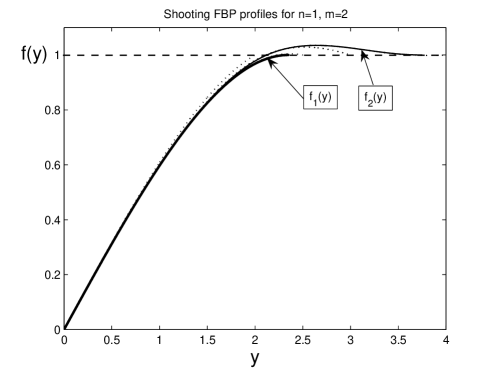
Figure 1. Construction of the unique first similarity profile $f_{1}(y)$ for the FBP.

2.4. On existence and uniqueness of the first monotone FBP $f_{1}$

We begin by mentioning that the mathematical techniques developed in Bernis [6] and Bernis–McLeod [8] as well as in [10, 26], are essentially directed to third-order ODEs obtained on integration ones via conservation laws, so these do not directly apply to the truly fourth-order ODE (1.17). Nevertheless, the methods and results therein can be useful. In particular, Bernis energy estimates [8, § 7] settles finite propagation property for such ODEs.

Shown in Figure 1 is the actual mathematical strategy to obtain the necessary profile $f_{1}(y)$ to get the following:

Proposition 2.3.

The problem $(\ref{4})$–$(\ref{6})$ admits a solution $f_{1}(y)$ satisfying

(2.56) $$f_{1}^{\prime}(y)>0,\,\,\,f_{1}^{\prime\prime}<0\quad\mbox{on}\quad(0,y_{0}),\quad\mbox{so}\quad 0<f_{1}(y)<1.$$

Proof. Thus, we shoot from the unknown interface point $y=y_{0}>0$ according to the bundle (2.2), and denote the solution as

(2.57) $$f=f(y;y_{0},C),$$

which can be continued until the regular point $y=0$. One can see that the ODE (1.17) does not admit local singularities at finite points. Our further analysis uses the continuous dependence of $f(y)$ on the parameters $y_{0}$ and $C$. Note that, as we have shown, the dependence is also continuous in the expansion (2.2) near singular (analytic) points.

We next need a few simple observations concerning such shooting orbits:

(i) We want to know that an inflection point of $f(y)$, where

(2.58) $$f^{\prime\prime}(y_{1})=0,\quad y_{1}\in[0,y_{0}),\quad f(y_{1})\in[0,1),$$

actually occurs. This is seen from the ODE and, moreover, from the expansion (2.2) that is obtained from it. Indeed, we have that, for $y\approx y_{0}^{-}$,

(2.59) $$f^{\prime\prime}(y)=-2C+\frac{1}{8}\,y_{0}(y_{0}-y)+...=0\,\,\,\mbox{at}\,\,\,y_{1}=y_{0}\big{(}1-\frac{16C}{y_{0}^{2}}+...\big{)},\quad\frac{C}{y_{0}^{2}}\ll 1.$$

The second condition in (2.58) then demands

$$f(y_{1}(y_{0}))=1-\frac{512}{3}\,\frac{C^{3}}{y_{0}^{2}}+...>0\quad\big{(}\frac{C^{3}}{y_{0}^{2}}\ll 1\big{)}.$$

Existence of $f_{1}(y)$ is proved if, for some $(y_{0},C)$,

(2.60) $$y_{1}=0.$$

(ii) We next use again the easy fact that follows from the ODE (1.17) that consists of two terms only with clear depending sign properties. Thus, (2.4) implies the positivity,

(2.61) $$-((1-f^{2})f^{\prime\prime\prime})(y)=\frac{1}{4}\,\int_{y}^{y_{0}}f^{\prime}y>0,$$

in a neighbourhood of $y_{0}^{-}$, where $f(y)$ is strictly increasing. Therefore, $f^{\prime\prime\prime}<0$ there, so that $f^{\prime\prime}(y)$ is strictly decreasing while $f^{\prime}(y)\geq 0$. Hence, we conclude that a monotone function $f(y)$ cannot have more than a unique inflection point $y_{1}=y_{0}(y_{0},C)$, at which (2.58) holds, in the connected domain of monotonicity of $f(y)$.

(iii) It is easy to see from (2.2) that, for any fixed $y_{0}>0$,

(2.62) $$f^{\prime\prime}<0\,\,\,\mbox{on}\,\,\,[0,y_{0})\,\,\,\mbox{provided that}\,\,\,C\gg y_{0}^{2},$$

so that the inflection point in (2.58) disappears for sufficiently large $C$. It is also easy to see that the type of disappearance of the point $I(y_{0},C)=(y_{1}(y_{0},C),f(y_{1}(y_{0},C)))$ from the domain $S_{1}=\{y>0,\,\,f\in(0,1)\}$ is different for $y_{0}\gg 1$ and $y_{0}\ll 1$. Namely, for $y_{0}\gg 1$, the point $I(y_{0})$ passes through the boundary axis $\{f=0\}$ as $C$ increases, while for $y_{0}\ll 1$, this is done through the boundary segment on $\{y=0\}$.

Using the above estimates, by continuous dependence on parameters $y_{0}$ and $C$ of this analytic family $\{f\}$, we conclude that there exists a $y_{0}>0$ such that (2.60) holds and the $f_{1}(y)$ satisfies (2.56). ∎

We expect that, in similar lines, there exists a proof of existence and uniqueness for higher-order TFEs leading to ODEs such as (1.32) that still contain two operators with related “signs”. Note that the total number of parameters increases with the order $2m$ so the shooting approach becomes more and more involved. For instance, for $m=3$, i.e., for the sixth-order TFE (1.30), we then have a three-parameter shooting, with parameters $f^{\prime}(0)$, $f^{\prime\prime\prime}(0)$, and $f^{(5)}(0)$. Nevertheless, the uniqueness of $f_{1}$ is surely observed in numerical experiments in Section 8.

2.5. On stability of the similarity solution in PDE setting

We now show how to check whether the similarity solution (1.16) with $f=f_{1}(y)$ is stable for the TFE (1.13) with respect to small perturbations of the data. We introduce the rescaled variables

(2.63) $$u(x,t)=v(y,\tau),\quad y=\frac{x}{t^{1/4}},\quad\tau=\ln t,$$

where $v$ solves the equation with the operator ${\bf B}$ from (1.17),

(2.64) $$v_{\tau}={\bf B}(v).$$

Since $\tau\to-\infty$ as $t\to 0$, where $u(x,t)$ approaches a slightly perturbed data $S_{+}(x)$, we need to show that these perturbations are exponentially decaying as $\tau$ increases. Thus, one needs to check the spectrum of the linearized operator

(2.65) $${\bf B}^{\prime}(f)Y=-((1-f^{2})Y^{\prime\prime\prime})^{\prime}+\big{(}\frac{y}{4}+2ff^{\prime\prime\prime}\big{)}Y^{\prime}+2(ff^{\prime\prime\prime})^{\prime}Y,$$

that is posed on $y\in(0,y_{0})$ with the anti-symmetry regular conditions at $y=0$,

(2.66) $$Y(0)=Y^{\prime\prime}(0)=0$$

and the free-boundary conditions

(2.67) $$Y=Y^{\prime}=0\quad\mbox{at}\quad y=y_{0}.$$

For simplicity of linear stability analysis, we assume that the free boundary is fixed at $=y_{0}$, so we exclude variation of the free boundary that are not principal.

Operator (2.65) is not symmetric in any space such as $L^{2}_{\rho}$, so it does not admit a self-adjoint extension. It is rather difficult degenerate singular operator that at the singular point $y=y_{0}$ has the principle part with a quadratic degeneracy according to (2.2),

$${\bf B}^{\prime}(f)Y=-2C((y_{0}-y)^{2}Y^{\prime\prime\prime})^{\prime}+...\,.$$

Therefore, solving the principle part of the eigenfunction equation,

(2.68) $$-2C((y_{0}-y)^{2}Y^{\prime\prime\prime})^{\prime}+...=\lambda Y\approx 0,$$

one obtains that the strongest singularity admitted by (2.68) is bounded,

(2.69) $$Y_{\rm s}(y)\sim(y_{0}-y)\ln(y_{0}-y)+...\quad\mbox{for}\quad y\approx y_{0}^{-}.$$

Obviously, the singular part (2.69) does not satisfy (2.67).

Hence, the conditions (2.67) themselves define an operator extension with a discrete spectrum. This follows from classic theory of ordinary differential operators [36], and also can be easily seen geometrically. Indeed, looking for eigenfunctions solving (2.68) is equivalent to shooting from the point $y=0$, where in view of (2.67) we are left with two parameters $Y^{\prime}(0)$ and $Y^{\prime\prime\prime}(0)$, and actually, since by linear scaling we can always put $Y^{\prime}(0)=1$ (if it is not zero, which is a special non-generic case). Therefore, the parameter $Y^{\prime\prime\prime}(0)\in{\mathbb{C}}$ together with $\lambda\in{\mathbb{C}}$ are, in general, sufficient to satisfy precisely two conditions (2.67) at $y=y_{0}$. This gives an analytic system for $\lambda$ [36], and shows that a compact resolvent in a suitable functional space as a meromorphic function is detected.

We restrict our attention to a necessary bound of the spectrum of (2.65),

(2.70) $${\bf B}^{\prime}(f)Y=\lambda Y.$$

As usual, multiplying this by the complex conjugate ${\overline{Y}}$ in $L^{2}$, taking the conjugate and multiplying by $Y$, and summing up both yields

(2.71) $$-\int(1-f^{2})\,|Y^{\prime\prime}|^{2}+\int[-(ff^{\prime})^{\prime}]\,|Y^{\prime}|^{2}+\int\big{[}(ff^{\prime\prime\prime})^{\prime}-\frac{1}{8}\big{]}\,|Y|^{2}=\frac{\lambda+\bar{\lambda}}{2}\int|Y|^{2}.$$

It is crucial that the first, highest-order term is negative, so the rest of the positive terms are expected to be estimated via interpolation. Actually, there are only two positive components: (i) in the second term:

(2.72) $$-(ff^{\prime})^{\prime}=-ff^{\prime\prime}-(f^{\prime})^{2},\quad\mbox{where}\quad-ff^{\prime\prime}>0\,\,\,\mbox{by}\,\,\,(\ref{95}),$$

and (ii) in the last term

(2.73) $$(ff^{\prime\prime\prime})^{\prime}=ff^{(4)}+f^{\prime}f^{\prime\prime\prime},\quad\mbox{where $f^{\prime}f^{\prime\prime\prime}<0$ but the sign of $ff^{(4)}$ is unknown}.$$

Note that close to $y=y_{0}$, the interpolation is possible regardless the degeneracy of the principle part in (2.71).

Thus we conclude from (2.71) that

(2.74) $${\rm Re}\,\lambda<0,$$

provided that a suitable (Friedrichs) self-adjoint extension of the following symmetric operator satisfies (a proper setting is standard, [36]):

(2.75) $${\bf Q}_{P}(f)Y=-[(1-f^{2})Y^{\prime\prime}]^{\prime\prime}+[(ff^{\prime})^{\prime}Y^{\prime}]^{\prime}+\big{[}(ff^{\prime\prime\prime})^{\prime}-\frac{1}{8}\big{]}Y<0.$$

For the first FBP profile $f_{1}(y)$, which is not given explicitly, (2.75) can be checked numerically and is rather plausible. At least, even without careful and not that easy spectral numerics, we observe that the self-adjoint operator in (2.75) exhibits a clear tendency to be negatively determined for reasonable FBP profiles $f=f_{1}(y)$ from (2.56).

3. The Cauchy setting for RP–$1$: oscillations and similarity profiles

We begin by noting that the CP setting for the TFE (1.12) assumes no analyticity unlike the TFE setting discussed in Section 2. For the CP, we observe oscillatory and changing sign behaviour near the interfaces.

3.1. Local solutions of changing sign

The oscillatory local behaviour for (1.17) is more complicated. Here we follow [24]. We introduce the oscillatory component $\varphi(s)$ as:

(3.1) $$f(y)=1-(y_{0}-y)^{3}\varphi(s),\quad s=\ln(y_{0}-y),$$

where $\varphi(s)$ solves an autonomous ODE with a discontinuous nonlinearity,

(3.2) $$\textstyle{P_{3}(\varphi)\equiv\varphi^{\prime\prime\prime}+6\varphi^{\prime\prime}+11\varphi^{\prime}+6\varphi=-\lambda_{0}\,{\rm sign}\,\varphi,\quad\mbox{where}\quad\lambda_{0}=\frac{1}{4}\,y_{0}>0.}$$

We look for a periodic solution of (3.2), which by (3.1) describes the oscillatory nature of solutions in the CP. Let us first note that technique based on calculation of rotation of vector fields for the dynamical system (3.2) does not apply here; see [35, p. 45-53]. In this case, existence of multiple periodic solutions depends on the careful analysis of the index of a guiding function $V$ (it always exists and can be calculated explicitly by using the linear form of the operator at infinity). Indices of such periodic solutions are unknown, the main results in [35, p. 52] seem not applicable for present problem.

Therefore, a direct shooting approach is effective here. We consider a 2D bundle of orbits $\varphi(s,C_{1},C_{2})$ satisfying the conditions

(3.3) $$\varphi(0)=0,\quad\varphi^{\prime}(0)=C_{1},\quad\varphi^{\prime\prime}(0)=C_{2},$$

where $C_{1,2}\in{\mathbb{R}}$ are arbitrary parameters. Let us state some key properties implying existence of a periodic orbit.

(i) $\varphi(s,C_{1},C_{2})$ is uniformly bounded for all $s>0$. Obviously, in view of boundedness of the nonlinearity, $\varphi(s,C_{1},C_{2})$ is locally well defined. If, on the contrary, $\varphi(s,C_{1},C_{2})$ is unbounded, we should have that the linear counterpart,

$$\varphi^{\prime\prime\prime}+6\varphi^{\prime\prime}+11\varphi^{\prime}+6\varphi=0,$$

must admit unbounded solutions. Setting $\varphi(s)={\mathrm{e}}^{\mu s}$ gives the characteristic equation

$$\Phi(\mu)\equiv\mu^{3}+6\mu^{2}+11\mu+6=0.$$

Since, $\Phi^{\prime}(\mu)>0$ for $\mu\geq 0$, $\Phi(0)=6$, and

$$\Phi^{\prime}(\mu)=0\quad\mbox{for}\quad\mu=\mu_{\pm}=\frac{1}{3}(6\pm\sqrt{3}),\quad\mbox{with}\quad\Phi(\mu_{\pm})=\mp 0.3849...\,,$$

we have that all three roots of $\Phi(\mu)$ are negative. So the solutions cannot grow without bound as $s\to+\infty$.

Actually, this means that, as a consequence, that the fourth-order ODE (3.2) with bounded coefficients is a dissipative DS having a bounded absorbing set. Dissipative DSs are known to admit periodic solutions in a rather general setting [35, § 39] provided these are non-autonomous (so the period is fixed). For the autonomous system (3.2), the proof in [24, § 7.1] can be completed by shooting.

(ii) $\varphi(s,C_{1},C_{2})$ is oscillatory as $s\to+\infty$, i.e., has infinite number of zeros in any neighbourhood of $s=+\infty$. Indeed, if, say, $\varphi(s,C_{1},C_{2})>0$ for all $s\gg 1$, we will have there the linear ODE

$$\varphi^{\prime\prime\prime}+6\varphi^{\prime\prime}+11\varphi^{\prime}+6\varphi=-1,$$

admitting the particular equilibrium solution $\varphi=-\frac{1}{6}$. Hence, by the above stability of the orbits of the homogeneous linear equation in (i), we conclude that $\varphi(s,C_{1},C_{2})\approx-\frac{1}{6}<0$ for all $s\gg 1$, from whence comes a contradiction.

We now state the main result.

Proposition 3.1.

(i) Equation $(\ref{k4})$ admits a unique non-trivial periodic solution $\varphi_{0}(s)$ of changing sign, which is stable as $s\to+\infty$; and

(ii) The periodic orbit $\varphi_{0}(s)$ of $(\ref{k4})$ is the unique bounded connection with $s=-\infty$.

Proof. (i) Existence and uniqueness have a pure algebraic proof, [24, § 7.4]. Stability follows from the above analysis of the linearized problem. (ii) This also implies that the stable manifold of $\varphi_{0}(s)$ as $s\to-\infty$ is empty, so, by the geometric analysis in [24], $\varphi_{0}(s)$ is the only bounded orbit connecting $s=-\infty$. ∎

Figure 2 shows that the periodic solution $\varphi_{0}(s)$ is stable, up to translations in $s$, as usual, for the ODE (3.2) as $s\to+\infty$.

In view of (ii), the expansion (3.1) with $\varphi=\varphi_{0}(s+s_{0})$, $s_{0}\in{\mathbb{R}}$ is arbitrary, is the only maximal regularity connection with $f(y)\equiv 0$ for $y>y_{0}$. Therefore, this describes the generic robust structure of the multiple zero at the interface of arbitrary similarity solutions of the TFE–4 under consideration. We expect that this structure remains unchanged for general solutions of the PDE (1.12), which is a difficult open problem. Observe that according to (3.1), the actual regularity of $f(y)$ is $C^{2,1}$ that is better than for the above FBP with the less smooth $C^{1,1}$ behaviour in (2.2) (if we formally set $f(y)\equiv 1$ for $y\geq y_{0}$). As we have mentioned, the regularity in (3.1) can be attributed to the Cauchy problems and in fact is the maximal regularity which is admitted by the ODE under consideration, [24].

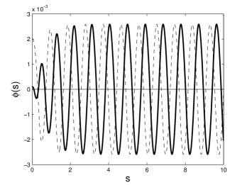
Figure 2. On the stable periodic orbit of (3.2), with $y_{0}=4$.

3.2. Similarity profile $f_{0}(y)$ for the CP

We begin by noting that finite propagation in the ODEs such as (1.17), i.e., existence of a finite interface $y_{0}$, is well-known for a long time; see first ODE proofs in [6, 8], and more general energy estimates for PDEs in [5, 41] and survey in [31].

As in the FBP, the bundle of asymptotics (3.1) is 2D comprising parameter $\{y_{0},s_{0}\}$, where $s_{0}$ is the translational constant in the oscillatory component, $\varphi_{0}(s)\mapsto\varphi_{0}(s+s_{0})$. Of course, the matching problem for the CP with the oscillatory bundle (3.1) gets more difficult.

In Figure 3, we show the unique similarity profile $f_{0}(y)$ corresponding to the CP. Figure 4 explains the character of oscillations of the $f(y)$ about $f=1$. This behaviour well-corresponds to the expansion (3.1). This shows a rough estimate of the interface location

(3.4) $$y_{0,{\rm CP}}\sim 6.7,$$

which is difficult to improve numerically in view of the oscillatory behaviour, the necessity of regularization parameters, and sufficiently low tolerance of convergence that was applied to the dynamical system (equivalent to (1.17)) with the essentially non-symmetric matrix.

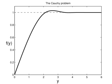
Figure 3. The CP profile $f_{0}(y)$ satisfying (1.17), (1.21).

(a) oscillations, enlarged

(b) oscillations, further enlarged

Figure 4. Enlarged oscillations of $f_{0}(y)$ from Figure 3 about the equilibrium $f=1$.

3.3. On a countable set of FBP profiles

Figure 1 indicates an interesting “geometric” relation between the first FBP profile and the CP one ($n=1$). For further convenience, in Figure 5, we present the enlarged version of this figure with extra details, where we include shooting of the third FBP profile $f_{3}(y)$ with interface positions at, respectively,

$$y_{01}\sim 2.35,\quad y_{02}\sim 3.75,\quad\mbox{and}\quad y_{03}\sim 4.74,$$

which all are smaller than the CP interface location (3.4). By boldface dotted line therein, we denote the CP profile $f_{0}(y)$.

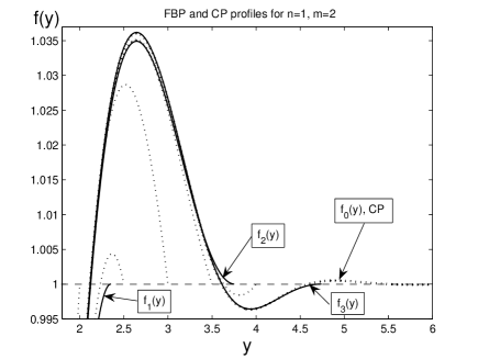
Figure 5. The CP $f_{0}(y)$ and first three FBP profiles for $n=1$.

Namely, we see that the touching point of $f_{1}(y)$ at the level $1$ belongs to the interval of the first oscillation of the profile for the CP, and the same is true for $f_{2}$ and $f_{3}$ in Figure 5. Moreover, we expect a further extension of this geometric property (an open problem).

Conjecture 3.2. The FBP $(\ref{4})$–$(\ref{6})$ admits a countable family of different solutions $\{f_{k}(y)\}$, where $f_{1}(y)\in[-1,1]$, which converges to the CP profile:

(3.5) $$f_{k}(y)\to f_{0}(y)\quad\mbox{as \,\, $k\to\infty$}$$

uniformly on any interval from $[0,y_{0,{\rm CP}})$.

In Figure 6, for clarity, we present a formal scheme of this geometric interaction between FBP and CP profiles, which partially has been reflected in Figure 5. This was already seen in Figures 1, 5, and will be clearer explained in Figure 14 obtained numerically for the TFE-6 ($m=3$ in (1.30)) admitting more oscillatory patterns. In particular, these figures show that the interface points $y_{0k}$ of the FBP profiles satisfy

(3.6) $$y_{0k}\to y_{0,{\rm CP}}^{-}\quad\mbox{as}\quad k\to\infty.$$

Recall that any FBP profile $f_{k}(y)$ being put into the similarity formula (1.16) gives a solution of the problem (1.12), (1.14). Therefore, in the FBP setting, Riemann’s problem for the TFE–4 has an infinite countable number of solutions (and only the first profile $f_{1}(y)$ has the physical range $[-1,1]$), while for the Cauchy setting, such a solution is expected to be unique (and violates the range $[-1,1]$).

\psfrag{f(y)}{$f(y)$}\psfrag{f_1(y), FBP}{$f_{1}(y)$, FBP}\psfrag{f_2(y), FBP}{$f_{2}(y)$, FBP}\psfrag{f_3(y), FBP}{$f_{3}(y)$, FBP}\psfrag{f_4(y), FBP}{$f_{4}(y)$, FBP}\psfrag{f(y), CP}{$f(y)$, CP}\psfrag{y_0CP}{$y_{0,{\rm CP}}$}\psfrag{1}{$1$}\psfrag{t4}{$t_{4}$}\psfrag{v(x,t-)}{$v(x,T^{-})$}\psfrag{final-time profile}{final-time profile}\psfrag{tapp1}{$t\approx 1^{-}$}\psfrag{y}{$y$}\psfrag{0<t1<t2<t3<t4}{$0<t_{1}<t_{2}<t_{3}<t_{4}$}\psfrag{0}{$0$}\psfrag{l}{$l$}\psfrag{-l}{$-l$}\includegraphics[scale={0.43}]{CPFBP.eps}

Figure 6. An extra schematic explanation of a countable set $\{f_{k}(y)\}$ of FBP profiles approaching the CP one (the bold line); cf. Figure 5.

4. On extension at the branching point $n=0$ in the Cauchy problem

Here, we demonstrate another approach to Riemann’s problem in the case of the Cauchy problem for the TFE-4 (1.22) with parameter $n\geq 0$. Then the similarity solution has the same form (1.16), there $f(y)$ solves the ODE

(4.1) $$\begin{matrix}{\bf B}_{n}(f)\equiv-(|1-f^{2}|^{n}f^{\prime\prime\prime})^{\prime}+\frac{1}{4}\,f^{\prime}y=0\quad\mbox{for}\quad y>0,\vskip 3.0pt plus 1.0pt minus 1.0pt\vskip 3.0pt plus 1.0pt minus 1.0pt\vskip 3.0pt plus 1.0pt minus 1.0pt\\ f(0)=f^{\prime\prime}(0)=0,\quad f(+\infty)=1.\end{matrix}$$

By our local analysis, we expect the solution with the finite interface to have a sufficiently regular connection with the equilibrium $f=1$, as explained in Section 3.

Our basic idea is to show that the solution of (4.1) can be extended from the solution $f_{0}$ in (1.28) of the linear problem for $n=0$, which then becomes a branching point for (4.1); see [35, p. 371]. To justify this, we will need some extra spectral properties of the linear operators involved.

4.1. Similarity profile and spectral properties of ${\bf B}$ for $n=0$

Thus, as we have seen, for $n=0$, the problem (4.1) in the CP setting takes the form

(4.2) $$\begin{matrix}{\bf B}_{0}(f)\equiv-f^{(4)}+\frac{1}{4}\,f^{\prime}y=0\quad\mbox{for}\quad y>0,\vskip 3.0pt plus 1.0pt minus 1.0pt\vskip 3.0pt plus 1.0pt minus 1.0pt\vskip 3.0pt plus 1.0pt minus 1.0pt\\ f(0)=f^{\prime\prime}(0)=0,\quad f(+\infty)=1,\end{matrix}$$

and has the unique solution $f_{0}(y)$ given in (1.28). It follows from (4.2) that

(4.3) $${\bf B}_{0}={\bf B}-\frac{1}{4}\,I,$$

where ${\bf B}$ is the linear operator in (1.26) that defines the rescaled kernel of the fundamental solution of the parabolic operator $D_{t}+D_{x}^{4}$.

The necessary spectral properties of the linear non self-adjoint operator ${\bf B}$ introduced in (1.26) and the corresponding adjoint operator ${\bf B}^{*}$ are of importance in the asymptotic analysis, as explained in [20] for similar general $2m$th-order operators (see also [23, § 4]). In particular, ${\bf B}$ is naturally defined in a weighted space $L^{2}_{\rho}({\mathbb{R}})$, with

$$\rho(y)={\mathrm{e}}^{a|y|^{4/3}},\quad\mbox{where \,$a\in(0,2d)$ \, is a constant},$$

with the domain being the corresponding Hilbert (Sobolev) space $H^{4}_{\rho}({\mathbb{R}})$. Then ${\bf B}:H^{4}_{\rho}({\mathbb{R}})\to L^{2}_{\rho}({\mathbb{R}})$ is a bounded operator and has the discrete (point) spectrum

(4.4) $$\sigma({\mathbf{B}})=\big{\{}\lambda_{l}=-\mbox{$\frac{l}{4}$},\,\,l=0,1,2,...\big{\}}.$$

The corresponding eigenfunctions are normalized derivatives of the rescaled kernel,

(4.5) $$\psi_{l}(y)=\frac{(-1)^{l}}{\sqrt{l!}}F^{(l)}(y),\quad l=0,1,2,...\,.$$

The adjoint operator

(4.6) $${\bf B}^{*}=-D_{y}^{4}-\frac{1}{4}\,yD_{y}$$

has the same spectrum (4.4) and the polynomial eigenfunctions

(4.7) $$\psi_{l}^{*}(y)=\frac{1}{\sqrt{l!}}\sum_{j=0}^{\lfloor-\lambda_{l}\rfloor}\frac{1}{j!}D^{4j}_{y}y^{l},\quad l=0,1,2,...,$$

which form a complete subset in $L^{2}_{\rho^{*}}({\mathbb{R}})$, where $\rho^{*}=\frac{1}{\rho}$. Similarly, the domain of the bounded operator ${\bf B}^{*}$ is the Sobolev space $H^{4}_{\rho^{*}}({\mathbb{R}})$. In particular, it is easy to compute

(4.8) $$\psi_{0}^{*}=1,\,\,\psi_{1}^{*}=y,\,\,\,\psi_{2}^{*}=\frac{1}{\sqrt{2}}\,y^{2},\,\,\,\psi_{3}^{*}=\frac{1}{\sqrt{6}}\,y^{3},\,\,\,\psi^{*}_{4}=\frac{1}{\sqrt{24}}\,(y^{4}+24),$$

etc. As ${\bf B}$, the adjoint operator ${\bf B}^{*}$ has the compact resolvent $({\bf B}^{*}-\lambda I)^{-1}$ in $L^{2}_{\rho^{*}}({\mathbb{R}})$. It is not difficult to see that, on integration by parts, the eigenfunctions (4.5) are orthonormal to polynomial eigenfunctions $\{\psi^{*}_{l}\}$ of the adjoint operator ${\bf B}^{*}$, so

(4.9) $$\langle\psi_{l},\psi^{*}_{k}\rangle=\delta_{lk},$$

where $\langle\cdot,\cdot\rangle$ denotes the standard (dual) scalar product in $L^{2}({\mathbb{R}})$.

Thus, in the necessary restriction to odd functions denoted by $L^{2}_{\rho}({\mathbb{R}}_{+})$, according to (4.3), we have that ${\bf B}_{0}$ has the discrete spectrum

(4.10) $$\sigma({\bf B}_{0})=\big{\{}-\frac{1+l}{4}\leq-\frac{1}{2},\,\,l=1,3,5,...\big{\}}$$

and a complete and closed set of eigenfunctions $\{\psi_{l}\}$. Hence, the linearized operator at $n=0$ is strictly negative in view of (4.10) that gives a good chance to extend the solution $f_{0}$ for $n>0$ small enough by applying classic branching theory in the study of the limit $n\to 0^{+}$ in the problem (4.1); see [46, p. 319] and [19, p. 381].

4.2. Branching at $n=0$

To this end, for $n>0$, we write down (4.1) as a perturbation of the linear problem (4.2),

(4.11) $${\bf B}_{0}f=g(f;n)\equiv\big{[}(|1-f^{2}|^{n}-1)f^{\prime\prime\prime}\big{]}^{\prime}.$$

Next, since ${\bf B}_{0}<0$ is known to have compact resolvent in $L^{2}_{\rho}({\mathbb{R}}_{+})$, we consider the equivalent integral equation for the function

(4.12) $$Y=f-f_{0},\quad\mbox{i.e.,}\quad f=f_{0}+Y,$$

which has the form

(4.13) $$Y={\bf A}(f_{0}+Y;n)\equiv{\bf B}_{0}^{-1}g(f_{0}+Y;n).$$

Initially, we formally assume that, for small $n\leq 1$, the nonlinear operator on the right-hand side can be treated as a compact Hammerstein operator in $L^{p}_{\rho}$-spaces, as classic theory suggests [35, § 17]. Recall that for $n=0$, (4.13) is indeed a linear integral equation with a compact operator admitting the unique (up to a multiplier) solution $f_{0}$ as in (1.28).

Therefore, performing below necessary computations, we bear in mind a formal use of classic branching theory for compact integral operators as in (4.13). We also do not discuss here specific aspects of compact integral operators in weighted $L^{p}$-spaces; see [20] for extra details. Note that, in a suitable metric, ${\bf B}$ is a sectorial operator, [27, § 5.1].

Therefore, for derivation of branching equations, we use general branching theory in Banach spaces; see Vainberg–Trenogin [46, Ch. 7]. Beforehand, we need to discuss a few typical difficulties associated with the above eigenvalue problem.

As (4.11) suggests, the crucial part is played by the nonlinearity

(4.14) $$Q(f;n)=|1-f^{2}|^{n}-1\quad\mbox{in a neighbourhood of the point $P_{0}=\{f=1,n=0^{+}\}$}.$$

One can see that the derivative $Q^{\prime}_{f}(f;n)$ is not continuous at $P_{0}$. Therefore, the standard implicit function (operator) theorem [46, p. 319] does not apply.

Nevertheless, the application of index-degree theory [35, p. 355] formally demands the differentiability only at the given point $f=f_{0}$, $n=0$, which is true (cf. more delicate computations below). Indeed, for $n=0$, $g(f,0)\equiv 0$, and the perturbation disappears in (4.13) at the branching point.

On the other hand, in view of our difficulties with the regularity (and also with compactness of the operators involved), it is better to rely on Theorem 28.1 in [19, p. 381] that is formulated in the linearized setting, where the differentiability is “replaced” by the control of higher-order nonlinear terms as in (4.14) in a neighborhood. As usual, the key principle of branching is that the corresponding eigenvalue has odd multiplicity that can be easily checked in some cases (the even multiplicity case needs an additional treatment, which is also a routine procedure not to be treated here); see further comments below. Notice that the condition on the nonlinearity (4.14) is rather tricky to check that it satisfies the estimate (b) in Theorem 28.1 in [19, p. 381] for the variable $x$ in $f=F+x$.

Thus, we can proceed and conclude that (4.1) admits a solution $f(y)$ for all sufficiently small $n>0$ and moreover these profiles form a continuous curve (an $n$-branch).

We next detect a precise behaviour of this branch as $n\to 0^{+}$.

4.3. Asymptotic expansion of the branch for small $n>0$

We need to use in (4.11) the following expansion:

(4.15) $$|1-f^{2}|^{n}-1=n\ln|1-f^{2}|+o(n)\quad\mbox{as}\quad n\to 0^{+},$$

which of course is not true uniformly on bounded intervals in $f$ and should be understood in the weak sense. This is crucial for the equivalent integral equation (4.13).

Proposition 4.1.

For the function $f=f_{0}$ given by $(\ref{s10})$, in the sense of distributions and in the weak sense in $L^{\infty}({\mathbb{R}}_{+})$ $($and also in the sense of bounded measures in ${\mathbb{R}}_{+})$

(4.16) $$\frac{1}{n}\,\big{(}\,|1-f^{2}|^{n}-1\,\big{)}\rightharpoonup\ln|1-f^{2}|\quad\mbox{as}\quad n\to 0^{+}.$$

According to (4.16), analyzing the integral equation (4.2), we can use the fact that, for any function $\phi\in{\mathcal{L}}$, $\phi\in L^{1}({\mathbb{R}}_{+})$ (or $\phi\in C_{0}({\mathbb{R}}_{+})$)

(4.17) $$\int(|1-f_{0}^{2}|^{n}-1)\phi(y)\,{\mathrm{d}}y=n\big{[}\int f(y)\ln|1-f_{0}^{2}(y)|\,\phi(y)\,{\mathrm{d}}y+o(1)\big{]}\,\,\,\mbox{as}\,\,\,n\to 0^{+}.$$

Let us finish our formal computations that, for convenience, are performed for the differential equation (4.1). Namely, substituting expansions (4.15) into (4.1) and using (4.12) yields the following perturbed equality:

(4.18) $${\bf B}_{0}Y=n(\ln|1-f_{0}^{2})f_{0}^{\prime\prime\prime})^{\prime}+o(n),$$

and this gives the unique solution

(4.19) $$Y=n{\bf B}_{0}^{-1}\big{[}(\ln|1-f_{0}^{2}|\,f_{0}^{\prime\prime\prime})^{\prime}\big{]}+o(n)\quad\mbox{as}\quad n\to 0.$$

One can see that

$$(\ln|1-f_{0}^{2}|\,f_{0}^{\prime\prime\prime})^{\prime}\in L^{2}_{\rho}({\mathbb{R}}_{+}),$$

so (4.19) makes sense. Thus, (4.12) and (4.19) actually determine the behaviour of the $n$-branch of similarity profiles of Riemann’s problem for sufficiently small $n>0$.

4.4. On global continuation of $n$-branches: open problem

Global continuation of branches of nonlinear eigenfunctions of (4.1) from the branching point is often an intriguing open problem. Global bifurcation results concerning continuous branches of solutions originated at $n=0$ are already given in Krasnosel’skii (the first Russian edition was published in 1956), [34, p. 196]. Concerning further results and extensions, see references in [19, Ch. 10] (especially, see [19, p. 401] for typical global continuation of bifurcation branches), and also [35, § 56.4].

In general, for the integral equation (4.13) with compact Hammerstein operators in weighted $L^{2}$-spaces, it is known since Rabinowitz’s study (1971) that branches are infinitely extensible and can end up at further bifurcation points; see [19, § 29] for further information stated in the framework of bifurcation analysis and [35, § 56.4]. The above $n$-extension of the branch is possible at any $n=n_{0}>0$ provided that the linearized operator has proper spectral properties. For oscillatory profiles $f(y)$ about $f=1$, with a complicated infinite set of intersection points, this is difficult to check in general but, in principle, can be done in specific weighted spaces, provided assuming that the oscillatory structure near interfaces is known in detail. Nevertheless, for the non-variational eigenvalue problem (4.1) with non-divergent and non-monotone operators, a rigorous treatment of global behaviour of branches is very difficult and remains open.

Since we have obtained the unique continuous branch originated at $n=0$, it will never come back to the origin, so this suggests that it can be extended up to $n=1$ and even further until homoclinic and other bifurcation points will destroy its necessary quality. Nevertheless, we do not know principles of such a global continuation, so we end up our branching analysis as follows:

Conjecture 4.1. The $n$-branch of nonlinear eigenfunctions of $(\ref{s1})$ that is originated at $n=0$ from $f_{0}$ exists for all $n\in[0,1]$ and does not have turning $($saddle-node$)$ points.

In Figure 7, we show the deformation with $n$, with the step $\Delta n=0.1$, of the CP similarity profile $f_{0}(y)$ satisfying (4.1). It is seen that all the profiles have quite similar shapes for $n=0$ (the dotted line) and $n=1$ including also the case of the negative exponents

$$n=-0.1,\,\,-0.2,\,\,-0.3,\,\,-0.4,\,\,-0.5,$$

for which $f_{0}(y)$ does not have finite interface but remains equally oscillatory as $y\to+\infty$. Figure 8 shows the enlarged oscillations about the constant equilibrium 1 of the profiles from Figure 7.

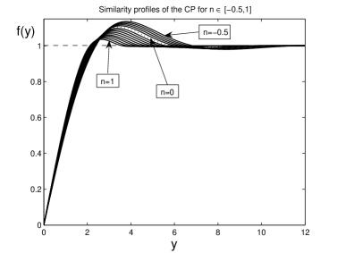
Figure 7. Continuous deformation in $n$ of similarity profiles satisfying (4.1); $n\in[-\frac{1}{2},1]$.

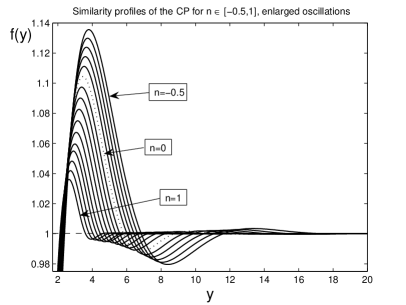
Figure 8. Enlarged oscillations of similarity profiles from Figure 7; $n\in[-\frac{1}{2},1]$.

5. Riemann problem $\frac{1}{2}$: similarity solutions

We now consider the RP–$\frac{1}{2}$ (1.17), (1.19), (1.20) or (1.21). Key aspects of the similarity analysis (both theoretical and numerical) are very similar. We stress the attention to some distinctive features.

In Figure 9, we show the unique similarity profile $f_{0}(y)$ of the RP–$\frac{1}{2}$ in the Cauchy setting. Notice that at the equilibrium level $f=1$ the similarity profile is clearly less oscillatory than at $\{f=0\}$, where propagation is approximately governed by the linear bi-harmonic PDE (1.24).

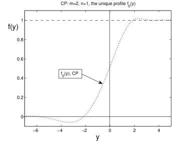
Figure 9. The CP solution of the RP–$\frac{1}{2}$ (1.17), (1.19), (1.21) for $n=1$.

Figure 10 shows in the enlarged scale first two FBP profiles for this RP–$\frac{1}{2}$ that are rather close to the CP one. The interfaces are

$$y_{01}\sim 2.07\quad\mbox{and}\quad y_{02}\sim 3.36.$$

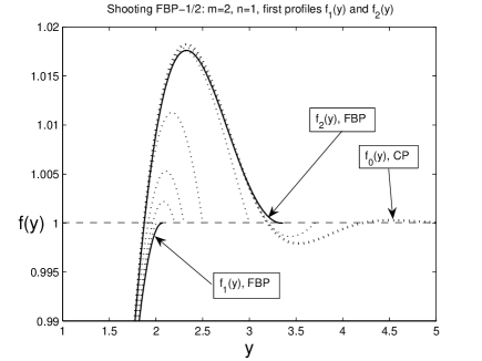
Figure 10. Two first FBP solutions of the RP–$\frac{1}{2}$ (1.17), (1.19), (1.20) for $n=1$.

The key aspects of homotopic connections and branching at $n=0$ for the RP–$\frac{1}{2}$ remain the same as for the RP–1. The only change is that, convoluting with Heaviside data (1.15) yields for $n=0$ the following similarity profile:

(5.1) $$f_{0}(y)=\int\limits_{-y}^{+\infty}F(z)\,{\mathrm{d}}z\quad(n=0).$$

6. Interface equations for the TFE–4 with unstable linear diffusion

We consider the TFE (1.33), and, studying finite propagation close to $u=1$, we set

$$1-u=v$$

to obtain, up to small perturbations, the following unstable TFE:

(6.1) $$v_{t}=-(|v|v_{xxx})_{x}-v_{xx}.$$

As usual, we take the simplest travelling wave (TW) solutions

(6.2) $$u(x,t)=f(y),\quad y=x-\lambda t\quad\Longrightarrow\quad-\lambda f^{\prime}=-(|f|f^{\prime\prime\prime})^{\prime}-f^{\prime\prime}.$$

Hence, on integration once assuming the zero flux condition at the interface at $y_{0}=0$,

(6.3) $$\lambda f=|f|f^{\prime\prime\prime}+f^{\prime}\quad\mbox{for}\quad y>0,\quad f(0)=0.$$

6.1. The FBP coincides with the CP

In the first approximation, we neglect the non-stationary term on the left-hand side of (6.3) and consider the equation

(6.4) $$|f|f^{\prime\prime\prime}+f^{\prime}=0\quad\mbox{for}\quad y>0,\quad f(0)=f^{\prime}(0)=0.$$

If $f^{\prime}(0)=0$, then the flux vanishes due to this ODE. Taking the expansion $f(y)=y^{2}\rho(y)$ and substituting into (6.4) we get $2\rho^{\prime}=-1+...\,.$ This gives the following first term expansion:

(6.5) $$f(y)=y^{2}|\ln y|+...\,.$$

Consider next the full equation (6.3). Dividing by $|f|$ and integrating yields

(6.6) $$\lambda y=f^{\prime\prime}+\ln|f|+C\quad(C\in{\mathbb{R}}).$$

Proposition 6.1.

${\rm(i)}$ Equation $(\ref{t7})$ does not admit oscillatory solutions near the interface at $y=0$; and

${\rm(ii)}$ $(\ref{t7})$ does not have a decaying solution with $f(+\infty)=0$.

In fact, (ii) shows that (6.6) does not admit infinite propagation (for TWs of course).

Proof. (i) Indeed, assuming that $f(y)\to 0$ as $y\to 0$, we have $\ln|f(y)|\ll-1$, so that $f^{\prime\prime}(y)>0$ and $f(y)$ is strictly convex in a neighbourhood. (ii) is straightforward. ∎

This means that the asymptotics (6.5) is already the actual maximal regularity behaviour corresponding to both the FBP and CP, which thus coincide for such a PDE.

The dynamic equation for the interface at $x=s(t)$ follows from (6.6) on differentiation, so we obtain the following equation with a third-order interface operator $S$:

(6.7) $$s^{\prime}(t)=\lambda=(f^{\prime\prime}+\ln|f|)^{\prime}=S[u]\equiv v_{xxx}+\frac{v_{x}}{v}\quad\mbox{at}\quad x=s(t).$$

A rigorous justification of such equations assumes using the von Mises variable $X(v,t)$ locally near sufficiently smooth and monotone interface,

$$X(v(x,t),t)=x,$$

though it leads to a number of technical difficulties; see [24].

7. Interface equations for the unstable nonlinear diffusion

We now treat the interface propagation for the equation (1.35), which, for $v=1-u\approx 0$, reduces to the standard TFE–4 with the unstable diffusion

(7.1) $$v_{t}=-(|v|v_{xxx})_{x}-(|v|^{m}v_{x})_{x}.$$

The TWs as in (6.2), on integration, yield the ODE

(7.2) $$\lambda f=|f|f^{\prime\prime\prime}+|f|^{m}f^{\prime}.$$

7.1. The FBP

Case I. The local analysis close to the interface at $y=y_{0}$ is pretty standard. Namely, we have got the pure TFE expansion like (2.2) [10, 26],

(7.3) $$f(y)=Cy^{2}+C_{1}y^{3}+...\,,\quad\mbox{where}\quad C_{1}=\frac{\lambda}{6},\quad C>0,$$

provided that

$$m>\frac{1}{2}.$$

This defines the standard interface equation

(7.4) $$s^{\prime}(t)=\lambda=6C_{1}\equiv v_{xxx}\quad\mbox{at \,\, $x=s(t)$}.$$

Case II. For the critical exponent $m=\frac{1}{2}$, all three terms in (7.2) are involved in the expansion yielding in (7.3)

$$C_{1}=\frac{\lambda}{6}-\frac{1}{3}\,C^{m}.$$

Therefore, the interface equation for TWs contains two operators

(7.5) $$s^{\prime}(t)=\lambda=S[u]\equiv v_{xxx}+2\bigl{(}\frac{1}{2}\,v_{xx}\bigr{)}^{m}\quad\mbox{at \,\, $x=s(t)$}.$$

Case III. Finally, for $m\in(0,\frac{1}{2})$, the FBP expansion is not $C^{3}$-smooth. For instance, in the first such range $m\in(\frac{1}{4},\frac{1}{2})$, the expansion is

(7.6) $$f(y)=Cy^{2}+C_{1}y^{2+2m}+\frac{\lambda}{6}\,y^{3}+...\,,\quad\mbox{where}\quad C_{1}=-\frac{1}{2m(1+m)(1+2m)}\,C^{m},$$

and, in the second term, the exponent satisfies $2<2+2m<3.$ Therefore, $f\not\in C^{3}([0,1])$, so the equality $\lambda=f^{\prime\prime\prime}(0)$ makes no sense and the interface equation becomes rather tricky. The simplest way to resolve (7.6) with respect to the speed $\lambda=s^{\prime}(t)$ is to decompose the TW solutions as follows:

$$v(x,t)=\hat{v}(x,t)+\tilde{v}(x,t),$$

where $\hat{v}(x,t)$ is $C^{3}$-smooth at the interface and $\tilde{v}(x,t)$ is not. Then the interface equation in this non-regular case takes the standard (similar to (7.4)) form

$$s^{\prime}(t)=(\hat{v})_{xxx}\quad\mbox{at}\,\,\,\,x=s(t).$$

An alternative, higher-order version can be obtained by observing from (7.2) that, for solutions (7.6),

$$\lambda Cy^{2}+...=ff^{\prime\prime\prime}+f^{m}f^{\prime}\quad\bigl{(}C=\frac{1}{2}\,f^{\prime\prime}(0)\bigr{)}.$$

Differentiating two times yields the following interface equation:

$$s^{\prime}(t)=S[u]\equiv\frac{1}{v_{xx}}\,(vv_{xxx}+v^{m}v_{x})_{xx}\quad\mbox{at}\,\,\,\,x=s(t).$$

The case $m=\frac{1}{4}$ is critical, where the second term on the right-hand side in (7.2) adds an extra operator into the interface equation that now reads (the above differential form is also available)

$$s^{\prime}(t)=(\hat{v})_{xxx}-\frac{8}{3}\bigl{(}\frac{1}{2}v_{xx}\bigr{)}^{2m-1}\quad\mbox{at}\,\,\,\,x=s(t).$$

A rigorous proof of such types of interface equations is a difficult open problem.

7.2. The CP

Case I. For $m>\frac{1}{3}$, the propagating ($\lambda<0$) TW solutions are oscillatory near interfaces and have the behaviour as in (3.1), i.e.,

(7.7) $$f(y)=y^{3}\varphi(s),\quad s=\ln y,$$

where $\varphi(s)$ is a periodic solution of the ODE (3.2) with $\lambda_{0}\mapsto-\lambda$.

Case II. In the critical case $m=\frac{1}{3}$, we still have the expansion (7.7), where the oscillatory component solves a different ODE,

(7.8) $$P_{3}(\varphi)=\lambda\,{\rm sign}\,\varphi-(\varphi^{\prime}+3\varphi)|\varphi|^{-\frac{2}{3}}.$$

Existence-uniqueness of a stable periodic orbit becomes harder and remains an open problem. Figure 11(a) shows the unique stable periodic solution of (7.8). In Figure (b), for comparison, we show the periodic behaviour in the ODE for the stable counterpart of the TFE with $m=\frac{1}{3}$,

(7.9) $$v_{t}=-(|v|v_{xxx})_{x}+(|v|^{\frac{1}{3}}v_{x})_{x}\,\,\Longrightarrow\,\,P_{3}(\varphi)=\lambda\,{\rm sign}\,\varphi+(\varphi^{\prime}+3\varphi)|\varphi|^{-\frac{2}{3}}.$$

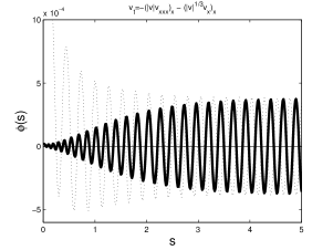
(a) unstable diffusion, $m=\frac{1}{3}$

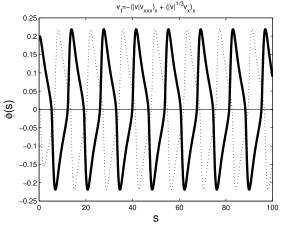
(b) stable diffusion, $m=\frac{1}{3}$

Figure 11. Stable periodic changing sign behaviour of the oscillatory component for the ODE (7.8) (a), and (7.9) (b); $\lambda=-1$.

Case III. Finally, in the range

$$0<m<{\rm min}\,\big{\{}\frac{1}{3},n\big{\}}$$

two terms on the right-hand side of (7.2) are leading that yields the same quadratic expansion (7.6) as in the FBP. It seems that, in this parameter range (and also for $m=0$ in Section 6), the CP and FBP settings coincide.

In the CP, in view of the oscillatory nature of solutions in most cases, even formal derivation of interface equations becomes difficult, to say nothing about their rigorous justification.

8. On higher-order TFEs: the RP–1 for $m=3$

Similarity solutions persist for higher-order TFEs (1.32). The matching becomes more-parametric and the topology of local bundles gets rather delicate. Numerics also get essentially more involved.

8.1. On the CP profile and oscillations

As an example, in Figure 12, we present the CP profile satisfying (1.32) for the case $m=3$ and $n=1$, i.e., for the sixth-order TFE (TFE–6). Instead of (3.1), the oscillatory behaviour about $f(y)\equiv 1$ is smoother,

(8.1) $$f(y)=1-(y_{0}-y)^{5}\varphi(s)+...\,,\quad s=\ln(y_{0}-y),$$

where $\varphi(s)$ solves a fifth-order ODE

(8.2) $$P_{5}(\varphi)\equiv\varphi^{(5)}+15\varphi^{(4)}+85\varphi^{\prime\prime\prime}+255\varphi^{\prime\prime}+\,274\varphi^{\prime}+120\varphi=\lambda_{0}\,{\rm sign}\,\varphi,$$

where $\lambda_{0}=\frac{1}{6}\,y_{0}$. See details on derivation in [25, § 12.2]. Figure 13 shows the unstable periodic solution of (8.2) for $\lambda_{0}=1$, which by (8.1) describes the oscillatory behaviour near the interface at

(8.3) $$y_{0,{\rm CP}}\sim 13.$$

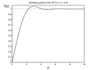
(a) CP profile

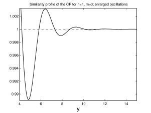
(b) oscillations, enlarged

Figure 12. The unique CP profile $f(y)$ solving (1.32), (1.21) for $m=3$, $n=1$; the profile (a), and enlarged oscillations about 1 (b).

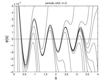
Figure 13. The trace of the unstable periodic orbit of (8.2), with $\lambda_{0}=1$ ($y_{0}=6$).

8.2. Shooting FBP profiles

The results of a standard shooting of the first FBP profiles are presented in Figure 14. Similar to shooting in Figure 1, here we have chosen the same strategy for higher-order equations: for $m=3$, we fix three free-boundary conditions from (1.33) excluding the second one, so changing the interface location $y_{0}$ as the free parameter, we want to satisfy the zero contact angle condition (2.54). As a consequence, we see in Figure 14 a consistent illustration of the limit FBP–CP process indicated earlier in the schematic Figure 6. Namely, we obtain four first FBP profiles, $f_{1}(y)$, $f_{2}(y)$, $f_{3}(y)$, and $f_{4}(y)$, with interfaces positions at

(8.4) $$y_{01}\sim 3.05,\,\,\,y_{02}\sim 4.85,\,\,\,y_{03}\sim 6.55,\,\,\,\mbox{and}\,\,\,y_{04}\sim 8.1.$$

These are smaller than the Cauchy one (8.3), which is expected to be the limit of all other FBP interfaces $\{y_{0k}\}$ as $k\to\infty$.

As usual, only the first profile $f_{1}(y)$ satisfies the physical range condition (1.23). Other profiles are oscillatory about the constant equilibrium $f=1$, and as it is seen in Figure 14, rather thoroughly mimic the oscillations of the linear solution (the boldfaced dotted line) defined by the same formula (1.28). This figure confirms that Conjecture 3.2 applies also to the TFE–6 (and seems to any of $2m$th-order ones (1.30)).

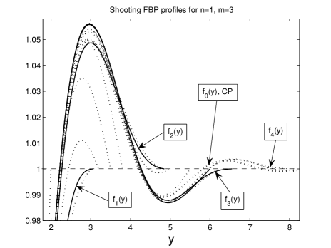
Figure 14. Shooting first four FBP profiles satisfying (1.32), (1.33) for $m=3$, $n=1$.

For comparison, in Figure 15, we present first three FBP profiles for the linear case $n=0$, i.e., $f$ solves the FBP

(8.5) $$\begin{matrix}f^{(6)}+\frac{1}{6}\,yf^{\prime}=0\quad\mbox{for}\quad y>0,\qquad\vskip 3.0pt plus 1.0pt minus 1.0pt\vskip 3.0pt plus 1.0pt minus 1.0pt\\ f(0)=f^{\prime\prime}(0)=f^{(4)}(0)=0,\quad f(y_{0})=1,\,\,\,f^{\prime}(y_{0})=f^{\prime\prime}(y_{0})=f^{(5)}(y_{0})=0.\qquad\end{matrix}$$

The interface positions are larger than that in (8.4) for $n=1$,

$$y_{01}\sim 3.29,\,\,\,y_{02}\sim 6.57,\,\,\,\mbox{and}\,\,\,y_{03}\sim 9.72.$$

Observe that the FBP profiles are close to corresponding humps of the CP profile denoted by the boldface dotted line. The general geometry of the mutual location of FBP and the CP profiles for $n=0$ is quite similar to the “nonlinear” one in Figure 14 for $n=1$ (the figures are topologically equivalent).

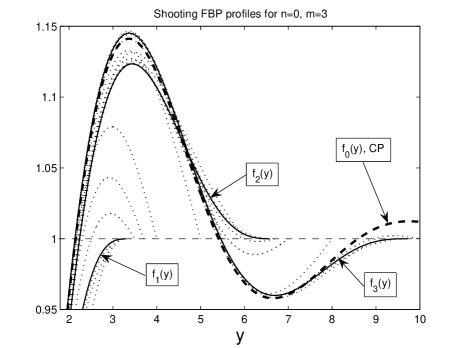
Figure 15. Shooting first three FBP profiles satisfying the linear FBP problem (8.5).

8.3. Branching at $n=0$

For $n=0$, (1.30) for $m=3$ becomes the tri-harmonic equation

(8.6) $$u_{t}=u_{xxxxxx}\quad\mbox{in}\quad{\mathbb{R}}\times{\mathbb{R}}_{+}.$$

Its fundamental solution is given by

(8.7) $$b(x,t)=t^{-\frac{1}{6}}F(y),\quad y=\frac{x}{t^{1/6}},$$

where $F$ is the unique symmetric solution of the problem

(8.8) $$\textstyle{{\bf B}F\equiv F^{(6)}+\frac{1}{6}\,F^{\prime}y+\frac{1}{6}\,F=0\quad\mbox{in}\quad{\mathbb{R}},\quad\int F=1.}$$

Extension of the similarity profiles of the ODE (1.32) from the branching point $n=0$ is the same as that for the TFE–4 in Section 4.1. Spectral properties of the corresponding linear operators ${\bf B}$ in (8.8) and the adjoint one

$${\bf B}^{*}=D_{y}^{6}-\frac{1}{6}\,yD_{y}$$

in $L^{2}_{\rho}({\mathbb{R}})$ and $L^{2}_{\rho^{*}}({\mathbb{R}})$ respectively can be found in [20].

In Figure 16, we show branching of the similarity profiles at $n=0$ (the dotted line), where, with the step $\Delta p=0.2$, we cover the range $p\in[-0.8,1]$. All the profiles are oscillatory, but for $n<0$ the interface is situated at $y_{0}=+\infty$.

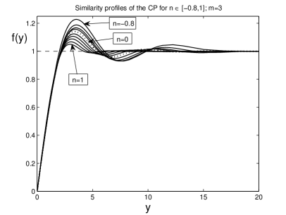
Figure 16. Similarity profiles of the CP satisfying (1.32) for $m=3$ appearing at the branching point $n=0$ (the dotted line).

Acknowledgements. The author would like to thank A. Novick-Cohen and A. Shishkov for discussions of the physical motivation of the problem for (1.13) and of some mathematical results respectively.

References

- [1] F.V. Atkinson and L.A. Peletier, Similarity profiles of flows through porous media, Arch. Rat. Mech. Anal., 42 (1971), 369–379.
- [2] F.V. Atkinson and L.A. Peletier, Similarity solutions of the nonlinear diffusion equation, Arch. Rat. Mech. Anal., 54 (1974), 373–392.
- [3] J.W. Barrett, J.F. Blowey, and H. Garcke, Finite element approximations of the Cahn–Hilliard equation with degenerate mobility, SIAM J. Numer. Anal., 37 (1999), 286–318.
- [4] E. Beretta, M. Bertsch, and R. Dal Passo, Nonnegative solutions of a fourth-order nonlinear degenerate parabolic equations, Arch. Ration. Mech. Anal., 129 (1995), 175–200.
- [5] F. Bernis, Finite speed of propagation and asymptotic rates for some nonlinear higher order parabolic equations with absorption, Proc. Roy. Soc. Edinburgh, 104A (1986), 1–19.
- [6] F. Bernis, Source-type solutions of fourth order degenerate parabolic equations, In: Proc. Microprogram Nonlinear Diffusion Eqs Equilibrium States, W.-M. Ni, L.A. Peletier, and J. Serrin, Eds., MSRI Publ., Berkeley, California, Vol. 1, New York, 1988, pp. 123–146.
- [7] F. Bernis and A. Friedman, Higher order nonlinear degenerate parabolic equations, J. Differ. Equat., 83 (1990), 179–206.
- [8] F. Bernis and J.B. McLeod, Similarity solutions of a higher order nonlinear diffusion equation, Nonl. Anal., TMA, 17 (1991), 1039–1068.
- [9] F. Bernis, Finite speed of propagation and continuity of the untergace for thin viscous flow, Adv. Differ. Equat., 1 (1996), 337–368.
- [10] F. Bernis, L.A. Peletier, and S.M. Williams, Source type solutions of a fourth order nonlinear degenerate parabolic equation, Nonl. Anal., TMA, 18 (1992), 217–234.
- [11] A.L. Bertozzi and M.C. Pugh, Long-wave instabilities and saturation in thin film equations, Comm. Pure Appl. Math., LI (1998), 625–651.
- [12] A.L. Bertozzi and M.C. Pugh, Finite-time blow-up of solutions of some long-wave unstable thin film equations, Indiana Univ. Math. J., 49 (2000), 1323–1366.
- [13] A. Bressan, Hyperbolic Systems of Conservation Laws. The One Dimensional Cauchy Problem, Oxford Univ. Press, Oxford, 2000.
- [14] J.W. Cahn, C.M. Elliott, and A. Novick-Cohen, The Cahn-Hilliard equation with a concentration dependent mobility: motion by minus the Laplacian of the mean curvature, Euro. J. Appl. Math., 7 (1996), 287–301.
- [15] D. Christodoulou,The Euler equations of compressible fluid flow, Bull. Amer. Math. Soc., 44 (2007), 581–602.
- [16] E.A. Coddington and N. Levinson, Theory of Ordinary Differential Equations, McGraw-Hill Book Company, Inc., New York/London, 1955.
- [17] C. Dafermos, Hyperbolic Conservation Laws in Continuum Physics, Springer-Verlag, Berlin, 1999.
- [18] R. Dal Passo and H. Garcke, Solutions of a fourth order degenerate parabolic equation with weak initial trace, Ann. Scuola Norm. Sup. Pisa Cl. Sci., (4) 28 (1999), 153–181.
- [19] K. Deimling, Nonlinear Functional Analysis, Springer-Verlag, Berlin/Tokyo, 1985.
- [20] Yu.V. Egorov, V.A. Galaktionov, V.A. Kondratiev, and S.I. Pohozaev, Asymptotic behaviour of global solutions to higher-order semilinear parabolic equations in the supercritical range, Adv. Differ. Equat., 9 (2004), 1009–1038.
- [21] S.D. Eidelman, Parabolic Systems, North-Holland Publ. Comp., Amsterdam/London, 1969.
- [22] C.M. Elliott and H. Garcke, On the Cahn–Hilliard equation with degenerate mobility, SIAM J. Math. Anal., 27 (1996), 404–423.
- [23] J.D. Evans, V.A. Galaktionov, and J.R. King, Blow-up similarity solutions of the fourth-order unstable thin film equation, Euro J. Appl. Math., 18 (2007), 195–231.
- [24] J.D. Evans, V.A. Galaktionov, and J.R. King, Source-type solutions of the fourth-order unstable thin film equation, Euro J. Appl. Math., 18 (2007), 273–321.
- [25] J.D. Evans, V.A. Galaktionov, and J.R. King, Unstable sixth-order thin film equation. I. Blow-up similarity solutions; II. Global similarity patterns, Nonlinearity, 20 (2007), 1799–1841, 1843–1881.
- [26] R. Ferreira and F. Bernis, Source-type solutions to thin-film equations in higher dimensions, Euro J. Appl. Math., 8 (1997), 507–534.
- [27] V.A. Galaktionov, Sturmian nodal set analysis for higher-order parabolic equations and applications, Adv. Differ. Equat., 12 (2007), 669–720.
- [28] V.A. Galaktionov, On higher-order viscosity approximations of odd-order nonlinear PDEs, J. Engr. Math., DOI 10.1007/s10665-007-9146-6.
- [29] V.A. Galaktionov, Shock waves and compactons for fifth-order nonlinear dispersion equations, Europ. J. Appl. Math., submitted.
- [30] V.A. Galaktionov and S.I. Pohozaev, Third-order nonlinear dispersion PDEs: shocks, rarefaction, and blow-up waves, Comput. Math. Math. Phys., to appear.
- [31] V.A. Galaktionov and A.E. Shishkov, Saint-Venant’s principle in blow-up for higher-order quasilinear parabolic equations, Proc. Royal Soc. Edinburgh, Sect. A, 133A (2003), 1075–1119.
- [32] V.A. Galaktionov and S.R. Svirshchevskii, Exact Solutions and Invariant Subspaces of Nonlinear Partial Differential Equations in Mechanics and Physics, ChapmanHall/CRC, Boca Raton, Florida, 2007.
- [33] V.A. Galaktionov and J.L. Vazquez, A Stability Technique for Evolution Partial Differential Equations. A Dynamical Systems Approach, Progr. in Nonl. Differ. Equat. and Their Appl., Vol. 56, Birkhäuser, Boston/Berlin, 2004.
- [34] M.A. Krasnosel’skii, Topological Methods in the Theory of Nonlinear Integral Equations, Pergamon Press, Oxford/Paris, 1964.
- [35] M.A. Krasnosel’skii and P.P. Zabreiko, Geometrical Methods of Nonlinear Analysis, Springer-Verlag, Berlin/Tokyo, 1984.
- [36] M.A. Naimark, Linear Differential Operators, Part II, Frederick Ungar Publ. Co., New York, 1968.
- [37] A. Novick-Cohen, The Cahn-Hilliard Equation: From Backwards Diffusion to Surface Diffusion, Cambridge Univ. Press, Cambridge, to appear.
- [38] A. Novick-Cohen and L.A. Segel, Nonlinear aspects of the Cahn-Hilliard equation, Physica D, 10 (1984), 277–298.
- [39] P.Ya. Polubarinova-Kochina, On a nonlinear differential equation encountered in the theory of filtration, Dokl. Akad. Nauk SSSR, 63, No. 6 (1948), 623–627.
- [40] B. Riemann, Über die Fortpfanzung ebener Luftwellen von endlicher Schwingungswete, Abhandlungen der Gesellshaft der Wissenshaften zu Göttingen, Meathematisch-physikalishe Klasse, 8 (1858-59), 43.
- [41] A.E. Shishkov, Dead cores and instantaneous compactification of the supports of energy solutions of quasilinear parabolic equations of arbitrary order, Sbornik: Math., 190 (1999), 1843–1869.
- [42] D. Slepev and M.C. Pugh, Self-similar blow-up of unstable thin-film equations, Indiana Univ. Math. J., 54 (2005), 1697–1738.
- [43] J. Smoller, Shock Waves and Reaction-Diffusion Equations, Springer-Verlag, New York/Berlin, 1983.
- [44] N.F. Smyth and J.M. Hill, High-order nonlinear diffusion, IMA J. Appl. Math., 40 (1988), 73–86.
- [45] C. Sturm, Mémoire sur une classe d’équations à différences partielles, J. Math. Pures Appl., 1 (1836), 373–444.
- [46] M.A. Vainberg and V.A. Trenogin, Theory of Branching of Solutions of Non-Linear Equations, Noordhoff Int. Publ., Leiden, 1974.
- [47] T.P. Witelski, A.J. Bernoff, and A.L. Bertozzi, Blow-up and dissipation in a critical-case unstable thin film equation, Euro J. Appl. Math., 15 (2004), 223–256.