On regularity of a boundary point for higher-order parabolic equations: towards Petrovskii-type criterion by blow-up approach

Abstract.

The classic problem of regularity of boundary points for higher-order PDEs is concerned. For second-order elliptic and parabolic equations, this study was completed by Wiener’s (1924) and Petrovskii’s (1934) criteria, and was extended to more general equations including quasilinear ones. Since the 1960–70s, the main success was achieved for $2m$th-order elliptic PDEs (e.g., by Kondrat’ev and Maz’ya), while the higher-order parabolic ones, with infinitely oscillatory kernels, were not studied in such great details.

As a basic model, explaining typical difficulties of regularity issues, the 1D bi-harmonic equation in a domain shrinking to the origin $(0,0)$ is concentrated upon:

$$u_{t}=-u_{xxxx}\quad\mbox{in}\quad Q_{0}=\{|x|<R(t),\,\,-1<t<0\},$$

where $R(t)>0$ is a smooth function on $[-1,0)$ and $R(t)\to 0^{+}$ as $t\to 0^{-}$. The zero Dirichlet conditions on the lateral boundary of $Q_{0}$ and bounded initial data are posed:

$$u=u_{x}=0\quad\mbox{at}\quad x=\pm R(t),\,\,-1\leq t<0,\quad\mbox{and}\quad u(x,-1)=u_{0}(x).$$

The boundary point $(0,0)$ is then regular (in Wiener’s sense) if $u(0,0^{-})=0$ for any data $u_{0}$, and is irregular otherwise. The proposed asymptotic blow-up approach shows that:

(i) for the backward fundamental parabolae with $R(t)=l(-t)^{1/4}$, the regularity of its vertex $(0,0)$ depends on the constant $l>0$: e.g., $l=4$ is regular, while $l=5$ is not;

(ii) for $R(t)=(-t)^{1/4}\varphi(-\ln(-t))$ with $\varphi(\tau)\to+\infty$ as $\tau\to+\infty$, regularity/irregularity of $(0,0)$ can be expressed in terms of an integral Petrovskii-like (Osgood–Dini) criterion. E.g., after a special “oscillatory cut-off” of the boundary, the function

$$\tilde{R}(t)=3^{-\frac{3}{4}}\,2^{\frac{11}{4}}(-t)^{\frac{1}{4}}\big{[}\ln|\ln(-t)|\big{]}^{\frac{3}{4}}$$

belongs to the regular case, while any increase of the constant $3^{-\frac{3}{4}}\,2^{\frac{11}{4}}$ therein leads to the irregular one. The results are based on Hermitian spectral theory of the operator ${\bf B}^{*}=-D_{y}^{(4)}-\frac{1}{4}\,\,yD_{y}$ in $L^{2}_{\rho^{*}}(\mathbb{R})$, where $\rho^{*}(y)={\mathrm{e}}^{-a|y|^{4/3}}$, $a={\rm constant}\in(0,3\cdot 2^{-\frac{8}{3}})$, together with typical ideas of boundary layers and blow-up matching analysis. Extensions to $2m$th-order poly-harmonic equations in $\mathbb{R}^{N}$ and other PDEs are discussed, and a partial survey on regulariy/irregularity issues is presented.

Dedicated to the memory of Professor I.G. Petrovskii

1. Introduction: Petrovskii’s regularity criterion (1934) and extensions

1.1. First discussion: regularity as a fundamental issue in potential theory

Well-posedness of initial-boundary value problems (IBVPs) for linear and nonlinear partial differential equations (PDEs) are key for general PDE theory and applications. The principal question, which was always in the focus of the key research in this area from the nineteenth century to our days, is to determine optimal, and as sharp as possible, conditions on the “shape” of the continuous boundary, under which the solution is continuous at the boundary points. This means that, for a given PDE with sufficiently smooth coefficients, a standard IBVP can be posed with a classical notion of solutions applied.

It is impossible to mention all the cornerstones of such regularity PDE theory achieved in the twentieth century. In the nineteenth century, this study, for the Laplace equation

(1.1) $$\Delta u=f\quad\mbox{in}\quad\Omega\subset\mathbb{R}^{2}\,\,\,\mbox{or}\,\,\,\mathbb{R}^{3}\quad(0\in\partial\Omega\,\,\,\mbox{is the point under scrutiny}),$$

began by Green (since 1828), Gauss (1940), Lord Kelvin (1847) and Dirichlet himself (in the 1850s), Weierstrass and Neumann (in the 1870s), Hilbert (1899), Schwarz, Poincaré (since 1887); see detailed history of potential theory in Kellogg [44, pp. 277–285]. It is also worth mentioning that classic in potential theory “Lyapunov’s surfaces” were introduced about 1898 for general non-convex domains in $\mathbb{R}^{3}$ (in the convex case, the problem was solved in 1870 by Karl Neumann). Lyapunov’s study was known to be inspired by Poincaré’s earlier papers; a full proof for general Lyapunov surfaces was completed by V.A. Steklov about 1902. As a related issue, as was pointed out by V.G. Maz’ya [69], Poincaré seems was the first who in last years of the nineteenth century already knew and used the exterior cone condition for the regularity of boundary points. As is well known from his private letters, discussions with several Russian mathematicians, including e.g., his supervisor P.L. Chebyshov and Steklov, Lyapunov was constantly rather anxious studying new and amazing but not fully rigorously justified ideas and methods by Poincaré. Possibly, this led him to develop the concept of “Lyapunov’s surfaces” in potential theory about that time (as well as some of other fundamental concepts in his stability theory, where discussions with Poincaré were also known to take place).

For the second-order Laplace equation (1.1) and the heat equation

(1.2) $$u_{t}=\Delta u\quad\mbox{in}\quad Q,\quad(0,0)\in\partial Q\,\,\mbox{is characteristic, where $\partial Q$ is tangent to $\{t=0\}$},$$

regularity theory was almost fully completed in the 1920–30s, and various ideas and key results on optimal regularity criteria created the amazing history, which is explained in a number of classic monographs. For convenience, we will begin our discussion with some historical aspects in next Section 3, where we hope to present some new and not that well-known regularity features and peculiarities for the sake of the attentive Reader.

The present paper uses the asymptotic blow-up approach from reaction-diffusion theory to such optimal boundary regularity questions. It is shown that, for a number of higher-order PDEs with essentially oscillatory kernels, these can be treated by blow-up evolution via approaching a “singular” boundary point. Surely, this is not a principal novelty not only for the heat equation (1.2) (Petrovskii, 1934), but also in elliptic regularity theory, where, together with other techniques, rescaled linear operator pencils were shown to be key; we refer to Kozlov–Maz’ya–Rossmann’s monographs [52, 53] and surveys in [27, 50, 68, 94] for details and full history. In this connection, Kondrat’ev’s seminal paper [49] for higher-order linear elliptic equations (see Kondrat’ev–Oleinik’s very detailed survey of 1983 [50] for up to the 1980s and the most recent monograph [12] for a huge number of more modern extensions), thought not devoted to the regularity issues, represented a novel and involved use of spectral properties of operator pencils for describing the asymptotics of solutions near corner singularities. This analysis assumes a kind of an “elliptic evolution” approach for elliptic problems, which then is not well-posed in Hadamard’s sense but can trace out the behaviour of necessary global orbits that approach the singularity point. For nonlinear elliptic equations, these ideas got various developments and diversions since the 1970s; see Véron’s monographs [91, 92] and [10] for further history and key references.

Classic Wiener’s and operator pencil ideas were successfully developed for many higher-order elliptic equations with a typical representative:

(1.3) $$(-\Delta)^{m}u=f\quad\mbox{in}\quad\Omega\subset\mathbb{R}^{N}\quad(m\geq 2),$$

in the papers by Maz’ya with collaborators since the 1970s; see e.g., [71] and [67, 68, 52, 53] as a guide. Though regularity point analysis for (1.3) revealed a lot of new phenomena and mathematical difficulties relative the classic ones for $m=1$ (see comments later on), there are many papers on this subject, where essential progress was achieved, especially in the recent ten years.

1.2. Higher-order parabolic PDEs: on some known regularity results

For $2m$th-order parabolic equations, where the basic model is the canonical poly-harmonic equation

(1.4) $$u_{t}=-(-\Delta)^{m}u,\quad\mbox{with}\quad m\geq 2,$$

regularity questions have been also addressed in the literature, however essentially less actively than for elliptic PDEs referred to above. Among results of classic solvability theory, which can be found in a number of monographs on linear and nonlinear equations, systematic approaches to the study of non-cylindrical domains with a characteristic vertex $(0,0)$, where the tangent plane $\{t={0}\}$ is horizontal in the $\{x,t\}$-space appeared already in the 1960s. V.P. Miha${\rm\check{i}}$lov papers in 1961 and 1963 [72, 73, 74] treated the case, where the parabolic boundary of the domain $Q_{0}$ lies below the characteristic plane $t=0$ and has a typical form of the corresponding “backward” paraboloid of the fundamental solution (in [73, 74], this shape is perturbed by factor that makes the paraboloid “sharper”, i.e., becomes “more regular”; see further comments on that). Almost simultaneously with the fundamental “elliptic” paper [49], Kondrat’ev in 1966 published another key “parabolic” paper [48], which is less known. Here, Kondrat’ev dealt with the singularity issues for more general than (1.4) parabolic equations and various boundary conditions on a fixed fundamental paraboloid. Complicated asymptotics of solutions near such singular points were obtained, and, as a result, a solvability criterion was proved for existence of weak solutions in special weighted Sobolev–Slobodetskii-type spaces. In 1971, Fe${\rm\check{i}}$gin [25] extended the results to the case when, in any neighbourhood of the vertex $(0,0)$, the boundary lies on both sides of the characteristic plane $\{t=0\}$ (see [85] for Fe${\rm\check{i}}$gin’s contribution to elliptic regularity theory in the 1970s). These deep results initiated further subsequent study, which nevertheless was not that exhaustive and sharp as in elliptic theory, and we will try to explain why (the answer seems easy: another level of difficulty). The current standing of this regularity parabolic theory can be traced out further by the MathSciNet, but the author reports that getting a clear convincing view is not easy.

1.3. Main goal: deriving sharp asymptotics of solutions near vertex depending on boundary geometry

As a consequence of the above discussion involving a number of strong previous results, obviously, optimal conditions of regularity/irregularity of the vertex $(0,0)$ for the poly-harmonic flow (1.4) demand the following:

(1.6) $$\begin{matrix}\mbox{{\bf Goal I}: \,\, sharp asymptotic expansion of solutions near $(0,0)$ are necessary}\qquad\vskip 3.0pt plus 1.0pt minus 1.0pt\\ \mbox{for rather arbitrary backward characteristic (non-fundamental) paraboloids}\vskip 3.0pt plus 1.0pt minus 1.0pt\\ \mbox{to get regularity ot the vertex {\em via} the geometry of the boundary nearby.}\qquad\end{matrix}$$

In other words, we check whether it is possible to characterize a sharp asymptotic behaviour of classic (strong) solutions near the characteristic vertex, when the paraboloid is not given by the backward variable of the fundamental solution, i.e., can take various forms. Loosely speaking, we are going to mimic a Petrovskii-type criterion for higher-order parabolic equations such as (1.4) (we must admit that, literally, this goal is not and cannot be achieved literally, but a partial progress is indeed doable). Once such an asymptotic has been obtained, one can re-evaluate the solution near the vertex in any necessary weighted metric, eventually to check whether solution exists (is continuous at the vertex) in weaker sense.

As usual, we find useful, in order to characterize our blow-up approach, to consider first the simplest 1D bi-harmonic equation

(1.7) $$u_{t}=-u_{xxxx}\quad(m=2),$$

which even in the one $x$-dimension provides us with a number of not that mathematically pleasant surprises. It seems that the main difference (and the origin of extra difficulties) between the higher-order elliptic case (1.3) and the parabolic one (1.7) is that the later has always oscillatory kernel of changing sign infinitely many times, while for (1.3), the kernel is less oscillatory and even remains positive in some dimensions even for $m\geq 2$. As is well known since Maz’ya–Nazarov’s results for $m=2$, $N\geq 8$ in 1986 [70], the changing sign kernels of elliptic operators produce new phenomena, where classic regularity techniques may fail and even standard conical points can be irregular (and singular, i.e., unbounded at the vertex). Note that Kondrat’ev’s sharp estimates such as (1.5) [49] can also indicate such a possibility, if sharp bounds on first pencil’s eigenvalues are known. Therefore, a simple 1D model (1.7) becomes a key parabolic PDE with such an infinitely oscillatory kernel, so we concentrate on this equation in what follows.

As a unified issue of the present analysis of higher-order parabolic and other PDEs (i.e., without any order-preserving or positive kernel features), we aim a sharp treatment of boundary regularity conditions by using spectral theory of related rescaled non self-adjoint operators or pencils of such operators. A full justification of some “approximate” regularity conditions are very difficult and lead to open problems. As an independent feature of the regularity questions, which underlines their difficult nature, as far as we know, even for the simplest higher-order elliptic or parabolic operators with real constant coefficients, there is a clear and natural difficulty for determining sufficiently sharp regularity conditions for linear operators with kernels of essentially changing sign. Of course, we exclude those operators for which the regularity is guaranteed by standard embedding results, or when the irregularity is induced by some symplectic–Hamiltonian properties, which do not allow any shrinking of the domain under consideration (e.g., the latter is true for Schrödinger operators ${\rm i}\,D_{t}+(-\Delta)^{m}$, where $L^{2}_{x}$-norm is preserved). For such operators, Wiener’s and other related capacity-like techniques, which assume kernel positivity, are naturally expected to fail, so new techniques are necessary.

Thus, our goal is to develop an asymptotic method of blow-up regularity analysis, firstly, for the simplest 1D bi-harmonic equation, and next extend to poly-harmonic ones (1.4). In general, together with other examples of PDEs, we follow the principle (as we have seen, such kernels have been studied much less in the mathematical literature)

(1.8) Goal II:   to deal with kernels having infinitely many sign changes,

that can occur not necessarily for parabolic PDEs only. We will show that a kind of Petrovskii-like integral “criterion” for regularity/irregularity of boundary points [81, 82] (1934–35) can be visualized. However, for operators with oscillatory kernels of changing sign, a standard deterministic analysis of such integral Osgood–Dini-type conditions via divergence/convergence (as for the second-order or other operators with more positively dominant kernels) is not available. Secondly, we discuss possible extensions of the method to other types of linear and nonlinear PDEs with the kernels like (1.8). Meantime, we continue our survey of the history of crucial for us regularity issues and integral criteria.

2. Elliptic equations as the origin of regularity theory: Zaremba (1911), Lebesgue (1913), and Wiener (1924)

2.1. Laplace equation: early days of existence and nonexistence theory

The first criterion (a necessary and sufficient condition) of regularity of a boundary point 0 was the Wiener famous one for the Dirichlet problem for the Laplace equation

$$\Delta u=f\,\,\,\mbox{in a bounded domain}\,\,\,\Omega\subset\mathbb{R}^{2},\,\,\,0\in\partial\Omega\quad\big{(}u=0\,\,\mbox{on $\partial\Omega$, for definiteness}\big{)},$$

derived in 1924, [93] (the case of arbitrary $N\geq 2$ was also embraced). It is formulated in terms of a diverging series of capacities (measuring the thickness of the complement of $\Omega$ near 0) of a discrete family of domains shrinking to the given point $0$ on the boundary; see extra details and further discussions in Courant–Hilbert [15, p. 306] and in Kellogg [44, p. 330].

Concerning nonexistence for the Dirichlet problem (see [66, 52, 53] for details), the first rigorous nonexistence example belonged to Stanislav Zaremba in 1911 [95, p. 310] (for a plane domain whose boundary has isolated points, not connected; e.g., the surface comprised a sphere and its centre); see comments in [44, p. 285]. The key non-solvability example was constructed by Lebesgue in 1913 [58, 59] who discovered striking examples of irregularity. E.g., he showed that, for a domain in $\mathbb{R}^{3}$ with the inner cone obtained by rotating the function $x_{2}={\mathrm{e}}^{-1/x_{1}}$ for $x_{1}>0$ small, about the $x_{1}$-axis (then the points with $x_{2}>{\mathrm{e}}^{-1/x_{1}}$ do not belong to the domain, i.e., the domain has a sharp cusp turned inwards, a Lebesgue spine), the origin 0 is irregular. Figuratively speaking, despite such a thin spine connection of the 0 with the boundary, “effectively” the centre remains “separated” reminding earlier Zaremba’s nonexistence construction. The same is true for $x_{2}=x_{1}^{|\ln x_{1}|^{\varepsilon}}$, with any $\varepsilon>0$ (0 is regular if it can be touched from outside by any cone given by rotation of $x_{2}=x_{1}^{k}$ for any $k>0$ fixed); see Petrovskii’s text book [83, p. 325]. Carleman’s PhD Thesis [13] of 1916 was also one of the first study of singularities of solutions of elliptic PDEs at non-regular boundary points; see also [50, Introd.].

Forty years later, new examples of nonexistence (somehow in lines with Zaremba–Lebesgue–Uryson’s ideas) were developed in [47, p. 129] by Kondrat’ev. For the Dirichlet problem $\Delta u+u=0$ in $\Omega$, he produced further examples of non-solvability for not simply connected domains for $N=2$ (sufficient number of disjoint small discs are removed), and domains in $\mathbb{R}^{3}$ such as a ball with line segments or narrow cylinders removed to get sufficiently small interior diameter (one end stays on the surface for not violating connectedness). These constructions extend to arbitrary $N$ and $2m$, including the most delicate range $N>2m$. By an $m$-capacity technique, [47] also studied the question of $k$-regularity ($k\leq m$) at a boundary point $A$ meaning that any $u\in W^{2}_{m,0}$ has $k-1$ derivatives vanishing there asymptotically (up to a set of the measure $o(a^{N})$ in $|x-A|<a$ as $a\to 0$).

2.2. Uryson (1924), Keldysh (1941), and Miusskaya Square

A nonexistence example similar to Lebesgue’s one was independently constructed by P.S. Uryson (1898–1924) in the early 1920s; his paper [89] was published in 1925, i.e., after his tragic death. From electrostatic point of view, which is natural for such problems, the electricity “flows down” from the cusp, i.e., cannot be retained there. Besides taking a physics curse from his PhD adviser N.N. Luzin (Luzin’s postgraduate course was completed by him in 1921), the physical intuition of Uryson was possibly created even before, when he, being in a gymnasium in Moscow, began to work at the Shanyavskii University in the Miusskaya Square, Moscow, under the supervision of the eminent Russian physicist P.P. Lasarev, and even published a paper on experimental research in X-radiation; see [6] (it seems less known that Uryson was the first, before Luzin, supervisor of A.N. Kolmogorov in his student’s period). This emphasizes Uryson’s outstanding physical motivation and understanding in the very early days of his scientific carrier. Both the Shanyavskii University and the Physical Institute, founded in 1911 for the outstanding physicist P.N. Lebedev (who first measured “pressure of the sun light”), were erected in 1910–1912 by Russian architect I.I. Ivanov-Schitz by using funding from Moscow’s merchants. Later on, since 1953, on the basis of Lebedev’s Institute building, was developed the Keldysh Institute of Applied Mathematics founded and headed until his death in 1978 by M.V. Keldysh.

Interestingly (and key for the whole comment), Keldysh made a significant and novel contribution to Dirichlet’s problem theory in 1941 in his celebrated paper [41] (see also [40]), which treated irregular points, as well as the new notion of stability of points and of the problem inside the domain relative perturbations of the boundary (the notion of capacity is discussed in Ch. II, while Ch. III is devoted to Wiener’s regularity criterion). In Ch. V, he proved that a stable boundary point is always regular, but the converse is not true (Keldysh balls $M$ were constructed having zero area of unstable points on $\partial M$ and of positive harmonic measure; see [37, 5] for a modern exhibition and extension).

It is also worth mentioning that ten years later, in 1951, Keldysh published the related paper [42] on elliptic equations that are degenerated on the boundary, where particularly the novel idea that a part of the boundary may be free from any conditions was introduced the first. These ideas were later developed by Fichera (since 1956), Oleinik, Radkevich, Kohn, Nirenberg (in the 1960s), etc.; see the monograph [79] and [14] for a more recent standing. For a full collection, let us mention Keldysh’s fundamental paper [43] (same 1951 year!) on linear operator pencil theory with applications to elliptic PDEs. Therein, several novel ideas including difficult $n$-fold completeness questions of root functions, i.e., eigen and associated ones, for the Keldysh pencils with variable coefficients, Keldysh chains, etc. were introduced. Its sequel in the 1950s includes works by I.M. Glazman, M.G. Krein, V.B. Lidskii, and others; these Keldysh methods of [43] were later used by Browder, Agranovich, Krukovsky, Agmon, Egorov, Kondrat’ev, Schulze, etc.; see [18] for details. The paper [43] was later classified as one of the main achievements of pencil theory in the twentieth century (together with J.D. Tamarkin’s results in his PhD Thesis in 1917, S.-Petersburgh’s University [88]); see Markus’ monograph [63] for the history and key results.

2.3. On some recent achievements

Since we are not dealing with elliptic equations in what follows, it is worth mentioning here that a full extension of Wiener’s regularity test (criterion) via the concepts of potential-theoretic Bessel (Riesz) capacities to $2m$th-order strongly elliptic equations with real constant coefficients,

(2.1) $$\left\{\begin{matrix}L(\partial)u=f,\quad f\in C_{0}^{\infty}(\Omega),\quad u\in H^{m}_{0},\qquad\qquad\qquad\qquad\qquad\qquad\quad\vskip 3.0pt plus 1.0pt minus 1.0pt\vskip 3.0pt plus 1.0pt minus 1.0pt\\ L(\partial)=\sum\limits_{|\alpha|=|\beta|=m}a_{\alpha\beta}\partial^{\alpha+\beta},\,\,a_{\alpha\beta}\equiv a_{\beta\alpha},\,\,\,(-1)^{m}L(\xi)>0\,\,\mbox{in}\,\,\mathbb{R}^{N}\setminus\{0\},\end{matrix}\right.$$

was completed in the case $N=2m$ in 2002 by Maz’ya ($N>2m$ also admits a treatment, though applied for a subclass of the so-called strongly elliptic equations; for $N\leq 2m-1$, the point is always regular by the classic Sobolev embeddings); see [67, 68] and references therein to earlier results and extensions.

Concerning the related questions of sharp asymptotic behaviour near Lipschitz boundary at 0 for problems (2.1), in [51], a rather general case of the boundary given by

$$\Omega=\big{\{}x=(x^{\prime},x_{n})\in\mathbb{R}^{N}:\quad x_{n}>\varphi(x^{\prime})\big{\}},\quad\varphi(0)=0,$$

is studied. The asymptotics as $x\to 0$ of a class of solutions are shown to depend on the Lipschitz constant of $\varphi(y^{\prime})$ in a neighbourhood of 0:

$$\textstyle{\kappa(\rho)=\sup_{|y^{\prime}|<\rho}\,|\nabla\varphi(y^{\prime})|\quad\big{(}\mbox{estimates are simplified if}\,\,\,\int_{0}\frac{\kappa^{2}(\rho)}{\rho}\,{\mathrm{d}}\rho<\infty\big{)}.}$$

Among others, let us also note an unusual Wiener’s-type regularity and existence result for blow-up on the boundary solutions of the semilinear elliptic equation

(2.2) $$\Delta u-|u|^{q-1}u=0\quad\mbox{in}\quad\Omega,\quad u(x)\to+\infty\quad\mbox{as}\quad x\to\partial\Omega\quad(q>1);$$

see [54, 62], where a long list of other related references is presented (equation (2.2) will be cited again).

3. Parabolic PDEs: Petrovskii’s $\sqrt{\log\log}$ criterion (1934) and around

3.1. Parabolic regularity theory began with the heat equation: first results and definitions

From the beginning, for the second-order parabolic equations, the boundary point regularity analysis took a different direction (i.e., not of Wiener’s type). This was Petrovskii [81, 82], who in 1934 completed the study of the regularity question for the 1D and 2D heat equation in a non-cylindrical domain. For further use, we formulate his result in a blow-up manner, which in fact was already used by Petrovskii in 1934 [81]. This is about the question on a irregular or regular point $(x,t)=(0,0)$ for nonnegative solutions of the IBVP

(3.1) $$\left\{\begin{matrix}u_{t}=u_{xx}\quad\mbox{in}\quad Q_{0}=\{|x|<R(t),\,\,\,-1<t<0\},\quad R(t)\to 0^{+}\,\,\mbox{as}\,\,t\to 0^{-},\vskip 3.0pt plus 1.0pt minus 1.0pt\vskip 3.0pt plus 1.0pt minus 1.0pt\vskip 3.0pt plus 1.0pt minus 1.0pt\\ \mbox{with bounded smooth data $u(x,0)=u_{0}(x)\geq 0$ on $[-R(-1),R(-1)]$}.\quad\,\,\,\end{matrix}\right.$$

Here the lateral boundary $\{x=\pm R(t),\,\,t\in[-1,0)\}$ is given by a function $R(t)$ that is assumed to be positive and $C^{1}$-smooth for all $-1\leq t<0$ and is allowed to have a singularity of $R^{\prime}(t)$ at $t=0^{-}$ only. We then study the value of $u(x,t)$ at the end “blow-up” characteristic point $(0,0^{-})$, to which the domain $Q_{0}$ is said to “shrink” as $t\to 0^{-}$.

For the heat equation, the first existence of a classical solution result was obtained by Gevrey in 1913–14 [34] (see Petrovskii’s references in [81, p. 55] and [82, p. 425]), which assumed that the Hölder exponent of $R(t)$ is larger than $\frac{1}{2}$, i.e., in our setting, at $t=0^{-}$, all types of boundaries given by the functions

(3.2) $$\framebox{$R(t)=(-t)^{\nu}\quad\mbox{with any $\nu>\frac{1}{2}$ are regular}\quad(\mbox{Gevrey, 1913--14}).$}$$

Note that, for $2m$th-order parabolic equations, a similar result saying that, for

(3.3) $$R(t)=(-t)^{\frac{1}{2m}},\quad\mbox{the problem is uniquely solvable}$$

(in Slobodetskii–Sobolev classes, i.e., not in the classic sense) was proved by Miha$\breve{\rm i}$lov [72] almost sixty years later.

Regular point: as usual in potential theory, the point $(x,t)=(0,0)$ is called regular (in Wiener’s sense, see [67]; sometimes is also called boundary) if any value of the solution $u(x,t)$ can be prescribed there by continuity as a standard boundary value on $\partial Q_{0}$. In particular, as a convenient and key for us evolution illustration, $(0,0)$ is regular if the continuity holds for any initial data $u_{0}(x)$ in the following sense:

(3.4) $$u=0\,\,\,\mbox{at the lateral boundary}\,\,\,\{|x|=R(t),\,-1\leq t<0\}\quad\Longrightarrow\quad u(0,0^{-})=0.$$

Irregular point: otherwise, the point is irregular (or inner) if the value $u(0,0^{-})$ is not arbitrary and is given by the parabolic evolution as $t\to 0^{-}$ (hence, formally and actually, $(0,0)$ does not belong to the parabolic boundary of $Q_{0}$, i.e., is inner in a natural sense).

3.2. On some details of Petrovskii’s analysis in 1934–35 and extensions

Reading last twenty five or so years various papers related to regularity issues for parabolic PDEs, the author found several and sometimes rather distinctive treatments of Petrovskii’s results. For instance, his 1934 paper [81] was not cited practically in no such papers, but the one [4]. There were also discrepancies in treating whether or not Petrovskii derived the integral Osgood–Dini-like conditions (surely, he did already in 1934). Therefore, we expect that it is worth mentioning here some aspects of Petrovskii’s original derivation of his celebrated criterion.

Thus, according to (3.1), in both cases of regularity/irregularity, there occur interesting asymptotic problems of the behaviour of $u(x,t)$ in $Q_{0}$ as $t\to 0^{-}$, which are of singular (finite-time blow-up) type. These problems were solved by Petrovskii [81, 82] in 1934–35, who derived a regularity criterion for (3.1) by constructing rather tricky sub- and super-solutions (“subparabolish” and ”superprabolish” in the original Petrovskii terminology, [82, p. 386]) of the heat equation.

For instance, to prove irregularity for the characteristic curve at $(0,0^{-})$

$$\textstyle{``\,\,x^{2}=4(1+\varepsilon)|t|\ln|\ln|t||\,\,",\quad\varepsilon>0,}$$

he introduced the following explicit sub-solution “Barriere der Irregularität” [81, p. 58], [82, p. 394] (see also comments in [76]):

(3.5) $$\textstyle{``\,\,\,v(x,t)=\frac{-1}{|\ln|t||^{1+\varepsilon_{1}}}\,\,{e}^{\frac{-x^{2}}{4t}\,k}+\frac{1}{\ln|\ln|t||}\,\,\,"\quad\big{(}v_{\,t}<v_{\,xx}\big{)},\quad\mbox{where}\quad\frac{1+\varepsilon_{1}}{k}<1+\varepsilon,}$$

and $\varepsilon_{1}<1$, $k<1$ are some positive constants. Vice versa, to prove regularity for

$$\textstyle{``\,\,\,x^{2}=4|t|\ln|\ln|t||\,\,\,",\quad(\mbox{i.e., $\varepsilon=0$}),}$$

the following explicit super-solution “Barriere der Regularität” [81, p. 58] was used:

(3.6) $$\textstyle{``\,\,\,v(x,t)=\frac{-1}{2|\ln|t||^{1\frac{1}{6}}}\,\,{e}^{\frac{-x^{2}}{4t}}+\frac{1}{\sqrt[6]{|\ln|t||}}\,\,\,"\quad\big{(}v_{\,t}>v_{\,xx}\big{)}.}$$

In [82], the standard nowadays notation $\underline{u}(x,t)$ and $\overline{u}(x,t)$ for sub- and super-solutions were used. For more general boundaries given by

(3.7) $$``\,\,\,x^{2}<4t\ln\rho(t)\,\,\,",$$

Petrovskii [82, p. 393] introduced the related function $\varphi(t)$ determined from

(3.8) $$\textstyle{``\,\,\,\int\limits_{t_{0}}^{t}\frac{\rho(\eta)d\eta}{\eta}=6\log\varphi(t)\,\,\,",}$$

which was used in constructing suitable super- and sub-solutions. Here, (3.8) is the origin of Petrovskii’s criteria (3.11) given below.

In his another paper [80] in 1934, Petrovskii also applied his novel method of sub- and super-solutions (i.e., before the classic Nagumo, or Müller–Nagumo–Westphal, Lemmas from the 1940-50s; for the Dirichlet problem, barrier-type ideas in the méthode de balayage, or sweeping out, were used by Poincaré as early as in 1887 [84], with further development by Lebesgue in 1912 [57] and by Perron in 1923 for $\Delta u=0$ [80, p. 432]) in the study of randomness that had a great influence on random processes theory, which he connected with linear elliptic equations. This role was first explained in Khinchin’s monographs in 1933 and 1936, [45]; see below. Note that, in [80], Petrovskii dealt with the Dirichlet problems (“Dirichletschen Problems”) for elliptic equations such as [80, p. 428]

$$\textstyle{``\,\,\,M_{xx}\frac{\partial^{2}u}{\partial x^{2}}+2M_{xy}\frac{\partial^{2}u}{\partial x\partial y}+M_{yy}\frac{\partial^{2}u}{\partial y^{2}}+2M_{x}\frac{\partial u}{\partial x}+2M_{y}\frac{\partial u}{\partial y}=0\,\,\,",}$$

where “$M_{xx}M_{yy}\geq M_{xy}^{2}$”, and, surely, Petrovskii’s typical double $\ln\ln$ appeared as an its solution “$u=\ln\ln\frac{1}{\sqrt{x^{2}+y^{2}}}$” on pp. 437–438. In three years time, sub-super-solution techniques were applied in the seminal KPP-paper, 1937 [46].

Petrovskii’s 1934’s paper [81] is fully devoted to the optimal regularity and existence-uniqueness analysis for the heat equation, where he already introduced his $2\sqrt{\ln\ln}$-criterion including the converging/diverging integral as in (3.11) for irregularity/regularity. For instance, he showed that the “5-$\log$ curve” and so on [81, p. 57] (cf. [82, p. 404])

$$\textstyle{``\,\,\,x^{2}=4|t|[\ln|\ln t||+1\frac{1}{2}\ln\ln|\ln|t||+\ln\ln|\ln|t||(1+\varepsilon)\ln\ln\ln\ln|\ln|t||]\quad\mbox{u. s. w.}\,\,"}$$

is regular for $\varepsilon\leq 0$ and is irregular for any $\varepsilon>0$. In addition, for the 2D heat equation

$$u_{t}=u_{xx}+u_{yy},$$

it is mentioned [81, p. 59] that the regularity/irregularity issues occur about the surface

$$``\,\,\,x^{2}+y^{2}=-4(1+\varepsilon)t\ln|\ln|t||\,\,\,".$$

In particular, then [82, p. 397] the super-solution took the same form (3.5), where $x^{2}$ is replaced by $x^{2}+y^{2}$. In the later paper [82] in 1935, extensions to the heat equation in $\mathbb{R}^{k}\times\mathbb{R}_{+}$ were mentioned.

Hence, we attribute Petrovskii’s criterion to 1934 [81], and not to 1935, [82], as used had been done in most of other “parabolic” regularity papers, we have referred to here. Concerning related earlier papers on parabolic PDEs in non-cylindrical domains, Solonnikov (1965) [87] and Ivasishen (1969) [38] should be mentioned.

Thus, using such novel barriers, Petrovskii [81, 82] established the following:

(3.9) $$\begin{matrix}{\rm(i)}\,R(t)=2\sqrt{-t}\,\,\sqrt{\ln|\ln(-t)|}\quad\Longrightarrow\quad\mbox{$(0,0)$ is regular},\quad\mbox{and}\quad\qquad\quad\vskip 3.0pt plus 1.0pt minus 1.0pt\\ {\rm(ii)}\,R(t)=2(1+\varepsilon)\sqrt{-t}\,\,\sqrt{\ln|\ln(-t)|},\,\,\varepsilon>0\quad\Longrightarrow\quad\mbox{$(0,0)$ is irregular}.\end{matrix}$$

More precisely, he showed that, for the curve expressed in terms of a positive function $\rho(h)\to 0^{+}$ as $h\to 0^{+}$ ($\rho(h)\sim\frac{1}{|\ln h|}$ is about right) as follows:

(3.10) $$\textstyle{R(t)=2\sqrt{-t}\,\,\sqrt{-\ln\rho(-t)},}$$

the sharp regularity criterion holds:

(3.11) $$\framebox{$\int\limits_{0}\frac{{\rho(h)}\sqrt{|\ln\rho(h)|}}{h}\,{\mathrm{d}}h<\,(=)\,+\infty\quad\Longrightarrow\quad\mbox{$(0,0^{-})$ is irregular (regular)}.$}$$

It is worth underlying again that both converging (irregularity) and diverging (regularity) integrals in (3.11) as Dini–Osgood-type regularity criteria already appeared in the first Petrovskii paper [81, p. 56] of 1934. It should be mentioned that, since Petrovskii used proposed him approach of constructing super- and sub-solutions, solving such partial differential inequalities led (as usual) unavoidably to a technical assumptions: for the super-solution (regularity of $(0,0)$), this is [82, p. 392]

$$``\,\,\,2.\quad t\log\rho(t)\to_{t\to 0}0;\,\,\,"$$

and, for the sub-solution (irregularity of $(0,0)$) [82, p. 397],

$$\begin{matrix}``\,\,\,3.\quad t\log\rho(t)\to 0\quad\mbox{f\"{u}r}\quad t\to 0;\,\,\,"\quad\mbox{and}\vskip 3.0pt plus 1.0pt minus 1.0pt\\ ``\,\,\,5.\quad\mbox{es ist}\quad\frac{\rho^{\prime}(t)}{\rho(t)}\leq\frac{1}{8|t|}.\,\,\,"\qquad\qquad\qquad\,\,\,\end{matrix}$$

These purely technical assumptions can be got rid of, [1]; our blow-up spectral-boundary layer approach is also assumptionless and rigorous for the heat equation, see Section 7.7.

The results of [81, 82] were key important for probability theory, where this result is expressed as follows: if $x_{t}$ is a 1D Wiener process and $\Phi(t)>0$ is monotone such that

(3.12) $$\textstyle{\int\limits^{\infty}\frac{\Phi(t)}{t}\,\,{\mathrm{e}}^{-\Phi^{2}(t)/2}\,{\mathrm{d}}t=\infty,}$$

then, with unit probability, $|x_{t}|\leq\Phi(t)$ for all $t\gg 1$. On the contrary (this is about the criterion), if the integral converges, then with unit probability $\exists\,\,\{t_{k}\}\to\infty$ such that $|x_{t_{k}}|>\Phi(t_{k})$; an optimal extension was done in [45]. Eventually, these Petrovskii’s results led to the so-called the Law of Iterated Logarithms (LIL) [16, p. 392], which was discovered by Khinchin and Kolmogorov. Earlier, in 1924 Khinchin proved that, for a sequence $\{X_{i}\}_{i\geq 1}$ of independent random variables with values $\pm 1$ with the probability $\frac{1}{2}$, there holds:

(3.13) $$S_{n}\equiv X_{1}+X_{2}+...+X_{n}\leq\sqrt{(2+\varepsilon)n\ln\ln n}\,\,\,\,\,\mbox{for all}\,\,\,n\gg 1\,\,\,(\forall\,\,\varepsilon>0)$$

with the probability one. This sharp estimate improved earlier Hausdorf’s inequality (1913) $S_{n}=o(n^{\frac{1}{2}+\varepsilon})$, Hardy–Littlewood’s one (1914) $S_{n}\leq C\sqrt{n\ln n}\,$, and Steinhaus’ inequality (1922) $\limsup S_{n}/\sqrt{2n\ln n}\leq 1$. As a final step, in 1929, Kolmogorov proved the LIL for any bounded independent random variables not assuming that the summands were identically distributed; see more details in [16, Ch. 7] and [35]. Clearly, (3.9) has probabilistic roots in (3.13).

A Wiener-type criterion, already established by Khinchin [45] (an earlier result was in 1933) in a probability representation, for the boundary regularity for problems such as (3.1) and in $\mathbb{R}^{N}$, was derived by Landis in 1969 [55] in terms of converging/diverging series of potentials of shrinking sets involved; see also [23] for a criterion via thermal capacity also obtained along the lines of derivation of Wiener’s one for Laplace’s equation. These results were not stated in the blow-up evolution and more “practical” Petrovskii’s style (3.11), though Wiener’s-type capacity criteria serve for more general types of boundaries than according to Petrovskii’s approach.

Petrovskii’s integral criterion of the Dini–Osgood type given in (3.11) is true in the $N$-dimensional radial case with (see [1]–[3] for the recent updating)

$$\sqrt{|\ln p(h)|}\quad\mbox{replaced by}\quad{|\ln p(h)|}^{\frac{N}{2}}.$$

Several boundary regularity/irregularity results are now known for a number of quasilinear parabolic equations including degenerate porous medium operators. Though, some difficult questions remain open even for the second-order parabolic equations with order-preserving semigroups. We refer to [1, 2, 3, 36, 61, 76] as a guide to a full history and the extensions of these important results.

As far as we know, (3.9) is the first clear appearance of the “magic” $\sqrt{\rm log\,log}$ in PDE theory, currently associated with the “blow-up behaviour” of the domain $Q_{0}$ and corresponding solutions. Concerning other classes of nonlinear PDEs generating blow-up $\sqrt{\rm log\,log}$ in other settings, see references in [30].

Finally, as an introduction to difficult features of higher-order parabolic regularity to be studied, it is worth clearly stating that

(3.14) for solutions of changing sign of the HE, Petrovskii’s criterion (3.11) fails

(obviously, positive subsolutions to prove irregularity are not applicable, while regularity can be still proved by comparison). In fact, a general criterion for arbitrary bounded changing sign data $u_{0}(x)$ in (3.1) cannot be derived in principle. The origin of this is the same for the HE (3.1), the bi-harmonic one (1.7), and others; see our analysis below.

3.3. Example: a refined asymptotics for the porous medium equation

In connection with the blow-up log-log, it is worth mentioning the asymptotic result (seems, unique of this type) for the Dirichlet problem as in (3.1) [36, § 2], which is now formulated for the radial porous medium equation in the pressure form:

(3.15) $$\begin{matrix}v_{t}=\Delta v^{m},\quad m>1,\quad\mbox{where the pressure $u=v^{m-1}$ solves:}\qquad\qquad\vskip 3.0pt plus 1.0pt minus 1.0pt\vskip 3.0pt plus 1.0pt minus 1.0pt\vskip 3.0pt plus 1.0pt minus 1.0pt\\ u_{t}=u\Delta u+\gamma|\nabla u|^{2}\quad\mbox{in}\quad Q_{0},\quad\mbox{with}\quad R(t)=\sqrt{-t},\quad\gamma=\frac{1}{m-1}>0.\qquad\qquad\end{matrix}$$

Then the log-log occurs in the asymptotic behaviour of nonnegative solutions as $t\to 0^{-}$:

(3.16) $$\textstyle{u(x,t)\sim\frac{1}{4\ln|\ln(-t)|}\to 0\quad\mbox{uniformly on subsets}\quad\big{|}\frac{|x|}{\sqrt{-t}}-1\big{|}\gg\frac{1}{\ln|\ln(-t)|}.}$$

The computations leading to (3.16) by asymptotic-matching ideas (some will be involved in our further study) are not easy, and a complete proof was not supplied in [36] (regardless the comment at the end of page 4 in [36], it seems that a full and entirely rigorous justification of this kind of matching with “floating” matching point can be extremely difficult and even seems illusive; this emphasizes a general complexity of such type of results even for second-order parabolic PDEs with the Maximum Principle).

Remark: on boundary criterion for (3.15). Obviously, the delicate asymptotics (3.16) allows one to detect the actual “criterion” of the boundary regularity for the equation (3.15) (strangely, this was not addressed in [36]). We use the scaling invariance of (3.15):

(3.17) $$u=A\,\hat{u},\quad x=\sqrt{A}{\hat{x}},\quad\mbox{where}\quad A>0\quad\mbox{is arbitrary}.$$

According to natural concepts of approximate similarity solutions (see e.g., [86, Ch. 6]), we next assume that

(3.18) $$A=A(t)\,\,\,\mbox{is not a constant, but a slow decaying function (relative to $\sqrt{-t}\,$).}$$

Then the equation for $\hat{u}(\hat{x},t)$ will include an extra very small asymptotic perturbation, which will not affect the asymptotics. Finally, according to (3.16) we set

(3.19) $$\textstyle{A(t)=\frac{1}{4\ln|\ln(-t)|},\quad\mbox{so that}\quad\hat{u}\sim 1}$$

on the corresponding compact subsets as $t\to 0^{-}$. Thus, $u(0,0)\not=0$ for the function

(3.20) $$\hat{R}(t)\sim 2\sqrt{-t}\,\sqrt{\ln|\ln(-t)|},$$

and, in this irregularity condition, Petrovskii’s magic $\sqrt{\ln\,\ln}$ again mysteriously occurs. The constant “2” here seems not relevant as in (3.9), since (3.15) is nonlinear and admits also the symmetry $u\mapsto Au,\quad t\mapsto\frac{t}{A}\quad\mbox{for any}\quad A>0,$ so that the domain behaviour with $\hat{R}(t)\sim\frac{2}{\sqrt{A}}\,\sqrt{-t}\,\sqrt{\ln|\ln(-t)|}$ is irregular for $(0,0)$.

* * *

Thus, since the 1930s, Petrovskii’s regularity $\sqrt{\log\log}$-factor entered parabolic theory and generated new types of asymptotic blow-up problems, which have been solved for a wide class of parabolic equations with variable coefficients as well as for some quasilinear ones. Nevertheless, such asymptotic problems are very delicate and some of them of Petrovskii’s type remain open even in the second-order case.

For higher-order poly-harmonic operators, the situation becomes much more difficult, since the Maximum and Comparison Principles and order-preserving properties fail, so classic barrier techniques associated with sub-, super-, and other solutions are not applicable in principle. This precisely reflects the area of the present research: no Maximum Principle tools, so that the boundary regularity problem in Petrovskii’s setting falls into the scope of a blow-up asymptotic behaviour study.

4. Towards Petrovskii’s criterion for the bi-harmonic flow: asymptotic blow-up setting, method, and layout of the paper

4.1. The basic Dirichlet problem under consideration

As a basic model, using the “minimal” extension of the heat equation (3.1) by increasing the order of the parabolic operator by two, we consider the bi-harmonic equation in the same shrinking domain as in (3.1) with the zero Dirichlet boundary conditions on the lateral boundary $\partial Q_{0}$:

(4.1) $$\left\{\begin{matrix}u_{t}=-u_{xxxx}\quad\mbox{in}\quad Q_{0}=\{|x|<R(t),\,\,\,-1<t<0\},\vskip 3.0pt plus 1.0pt minus 1.0pt\vskip 3.0pt plus 1.0pt minus 1.0pt\\ u=u_{x}=0\quad\mbox{at}\quad x=\pm R(t),\quad-1\leq t<0,\quad\,\,\,\,\,\,\,\,\,\,\vskip 3.0pt plus 1.0pt minus 1.0pt\vskip 3.0pt plus 1.0pt minus 1.0pt\\ u(x,0)=u_{0}(x)\quad\mbox{on}\quad[-R(-1),R(-1)],\qquad\quad\,\,\,\,\,\,\,\,\end{matrix}\right.$$

where $u_{0}(x)$ is a bounded and smooth function, $u_{0}(\pm R(-1))=0$.

First of all, obviously, in modern PDE theory, there are many very strong regularity results, proved for wide classes of linear and nonlinear equations including, of course, the simplest among others bi-harmonic one (4.1). We have mentioned some key results and papers before and will not indent to compete with those nice results and present no further references to this classic literature. The only issue we propose here is as follows: to show how to derive

(4.2) a sharp boundary regularity criterion for (4.1) as a blow-up problem.

As we have seen, these blow-up aspects of the regularity problem were already clearly revealed by Petrovskii in 1934. Though, for the second-order case, there are other equivalent approaches based on the positivity of the kernel and various order-preserving features, which fail for oscillatory kernels.

To be more precise, this blow-up study for (4.1) is performed for:

(4.3) a generic class of solutions exhibiting a “centre subspace” behaviour.

In other words, as our Hermitian spectral theory of higher-order non self-adjoint linear operators in Section 5 shows, one can expect that, in addition to (4.3),

(4.4) $$\begin{matrix}\exists\,\,\,\,\mbox{an infinite-dimensional set of ``stable manifold" patterns,}\vskip 3.0pt plus 1.0pt minus 1.0pt\\ \mbox{for which the conditions of regularity of $(0,0)$ are all different.}\end{matrix}$$

It is principal for us that, to confirm the optimal character of the class of generic blow-up asymptotics, we will check (Section 7.7) that, by elementary spectral calculus,

(4.5) $$\begin{matrix}\mbox{the same asymptotic approach to the classic problem (\ref{ir1}) by classic}\qquad\quad\vskip 3.0pt plus 1.0pt minus 1.0pt\\ \mbox{Hermite spectral theory yields precisely Petrovskii's criterion in (\ref{RR1}).}\qquad\quad\end{matrix}$$

Note that the problem: (4.3) or (4.4), also exists for the heat equation (3.1) (cf. (3.14)), but here, by the Maximum Principle, positive solutions always belong to the generic class (4.3). For the bi-harmonic PDE (4.1), in a general setting, distinguishing generic patterns (4.3) from those in (4.4) is difficult and seems even impossible (or makes no sense).

4.2. Slow growing factor $\varphi(\tau)$

Thus, similar to (3.9), we need to assume that

(4.6) $$R(t)=(-t)^{\frac{1}{4}}\,\varphi(\tau),\quad\mbox{where}\quad\tau=-\ln(-t)\to+\infty\quad\mbox{as}\quad t\to 0^{-}.$$

Here, the scaling main factor $(-t)^{1/4}$ naturally comes from the bi-harmonic kernel variables (see (4.11) and (5.3)), and $\varphi(\tau)>0$ is an unknown slow growing function satisfying

(4.7) $$\textstyle{\varphi(\tau)\to+\infty,\quad\varphi^{\prime}(\tau)\to 0,\quad\mbox{and}\quad\frac{\varphi^{\prime}(\tau)}{\varphi(\tau)}\to 0\quad\mbox{as}\quad\tau\to+\infty.}$$

Moreover, as a sharper characterization of the above class of slow growing functions, we use the following criterion:

(4.8) $$\textstyle{\big{(}\frac{\varphi(\tau)}{\varphi^{\prime}(\tau)}\big{)}^{\prime}\to\infty\quad\mbox{as}\quad\tau\to+\infty\quad(\varphi^{\prime}(\tau)\not=0).}$$

This is a typical condition in blow-up analysis distinguishing classes of exponential (the limit is 0), power-like (a constant $\not=0$), and slow-growing functions. See [86, pp. 390-400], where in Lemma 1 on p. 400, extra properties of slow-growing functions (4.8) are proved. For instance, one can derive the following comparison of such $\varphi(\tau)$ with any power:

(4.9) $$\mbox{for any $\alpha>0$},\quad\varphi(\tau)\ll\tau^{\alpha}\quad\mbox{and}\quad\varphi^{\prime}(\tau)\ll\tau^{\alpha-1}\quad\mbox{for}\quad\tau\gg 1.$$

Such estimates are useful in evaluating perturbation terms in the rescaled equations.

Thus, the monotone positive function $\varphi(\tau)$ in (4.6) is assumed to determine a sharp behaviour of the boundary of $Q_{0}$ near the shrinking point $(0,0)$ to guarantee its regularity. In Petrovskii’s criterion (3.9), the almost optimal function, satisfying (4.7), (4.8), is

(4.10) $$\varphi_{1}(\tau)\sim 2\sqrt{\ln\tau}\quad\mbox{as}\quad\tau\to+\infty,$$

a dependence we have to compare our final results for the bi-harmonic equation with.

4.3. First kernel scaling and layout

By (4.6), we perform the similarity scaling

(4.11) $$\textstyle{u(x,t)=v(y,\tau),\quad\mbox{where}\quad y=\frac{x}{(-t)^{1/4}}.}$$

Then the rescaled function $v(y,\tau)$ now solves the rescaled equation

(4.12) $$\left\{\begin{matrix}v_{\tau}={\bf B}^{*}v\equiv-v_{yyyy}-\frac{1}{4}\,yv_{y}\quad\mbox{in}\quad Q_{0}=\{|y|<\varphi(\tau),\,\,\,\tau>0\},\vskip 3.0pt plus 1.0pt minus 1.0pt\vskip 3.0pt plus 1.0pt minus 1.0pt\\ v=v_{y}=0\quad\mbox{at}\quad y=\pm\varphi(\tau),\,\,\tau\geq 0,\qquad\qquad\qquad\qquad\qquad\,\vskip 3.0pt plus 1.0pt minus 1.0pt\vskip 3.0pt plus 1.0pt minus 1.0pt\\ v(0,y)=v_{0}(y)\equiv u_{0}(y)\quad\mbox{on}\quad[-R(-1),R(-1)].\qquad\quad\,\,\,\,\,\,\,\,\,\,\,\,\end{matrix}\right.$$

In view of the divergence (4.7), it follows that our final analysis will essentially depend on the spectral properties of the linear operator ${\bf B}^{*}$ on the whole line $\mathbb{R}$. We reflect this Hermitian spectral theory in the next Section 5, with application to the regularity criterion in Section 7. In particular, this differs our analysis from Kondrat’ev’s classic one [48].

However, in Section 6, we begin the study of the regularity of the vertex $(0,0)$ of the bi-harmonic backward fundamental parabolae:

(4.13) $$R(t)=l(-t)^{\frac{1}{4}},\quad\mbox{i.e.,}\quad\varphi(\tau)\equiv l={\rm const.}>0.$$

Then the problem (4.12) is considered on the fixed interval $I_{l}=\{|y|<l\}$, so that the final conclusion entirely depends on spectral properties of ${\bf B}^{*}$ in $I_{l}$ with Dirichlet boundary conditions. Of course, then the spectral problem for ${\bf B}^{*}$ (not a pencil) becomes a very particular case of the general setting developed in [48], but nevertheless, the clear conclusion on regilarity/irregularity becomes rather involved, where numerics are necessary to fix final details. In addition, as we pointed out, in more general setting for the fundamental backward paraboloids in $\mathbb{R}^{N}$, the existence, uniqueness, and regularity of solutions in Sobolev spaces was proved in a number of papers such as [72, 73, 74, 25], etc. Note that in [73, p. 45], the zero boundary data was understood in the mean sense (i.e., in the $L^{2}$-sense along a sequence smooth internal contours “converging” to the boundary). Nevertheless, we have to stress attention to this simple case in order to reveal the exact transition between regularity and irregularity in the classic sense in the critical case (4.13). It seems that such a border case in between was not addressed before sharply enough.

Thus, our conclusion is rather disappointing: unlike the classic heat equation (3.1), for the bi-harmonic equation (4.1), the vertexes of the fundamental parabolae (4.13) are not necessarily regular. For instance, on the basis of careful numerics, we show that:

(4.14) $$\framebox{$\begin{matrix}R(t)=4(-t)^{\frac{1}{4}}\quad\Longrightarrow\quad\mbox{$(0,0)$ is regular, while}\vskip 3.0pt plus 1.0pt minus 1.0pt\vskip 3.0pt plus 1.0pt minus 1.0pt\\ R(t)=5(-t)^{\frac{1}{4}}\quad\Longrightarrow\quad\mbox{$(0,0)$ is irregular.}\qquad\end{matrix}$}$$

Moreover, in the latter case, the vertex $(0,0)$ is singular, i.e.,

(4.15) $$\mbox{in general, $u(x,t)$ is unbounded as $(x,t)\to(0,0^{-})$}.$$

We also claim that (by a continuity argument) there exists some $l_{1}\in(4,5)$ such that $(0,0)$ is irregular, but not singular, i.e., the limit $u(0,0^{-})$ exists.

These regularity variations for constant functions $\varphi(\tau)\equiv l$ inevitably impose a special restriction for the study in Section 7 unbounded $\varphi(\tau)$’s satisfying (4.7), where we derive a Petrovskii-like “criterion” of regularity. Namely, the irregularity condition is obtained in terms of an Osgood–Dini-type integral condition, while, in an accordance with (4.14), for the regularity, a special “oscillatory cut-off” of the lateral boundary must be applied.

In Section 8, we discuss the extensions of the boundary regularity analysis to $2m$th-order poly-harmonic operators

(4.16) $$u_{t}=(-1)^{m+1}D_{x}^{2m}u\quad\mbox{in}\quad Q_{0}\quad(m\geq 2),$$

with the zero Dirichlet conditions, as well as for the same $N$-dimensional problem for (1.4) in $Q_{0}$, where the shape of the shrinking domain $Q_{0}$ is also of importance for the boundary regularity. For instance, one can consider the radial $Q_{0}$ given in (4.1), where $|x|$ stands for the radial spatial variable. We also discuss regularity conditions for the third-order linear dispersion equations, for a quasilinear fourth-order porous-medium-type equation (the PME–4), and for the linear wave (beam) equation of the fourth order.

The present paper aims to give a first insight into principal difficulties of a sharp study of boundary regularity for higher-order parabolic and other evolution PDEs. Such a study inevitably generates a number of difficult mathematical problems, which, partially, do not appear in the second-order case, or can be avoided by positivity kernel properties. We must admit that some of them are not and even cannot be completely rigorously solved. The main problem of concern is that distinguishing generic patterns in (4.3) from non-generic ones in (4.4) is not possible in general. Here, delicate boundary layer theory is essentially involved, where we ought to use some accurate numerical calculations by the MatLab whenever necessary to avoid huge technical digressions (using those seems also inevitable for truly $2m$th-order parabolic equations with large enough $m\geq 2$). Regardless a certain rigorous incompleteness of the mathematical analysis in some steps (which seems to be inevitable in general), we decide to demonstrate the whole machinery of the asymptotic blow-up methods in parabolic boundary regularity theory, and hope that this will help to attract some attentive Readers to improve the results when necessary. It is worth mentioning that, as can be seen in many directions of modern PDE theory of linear and nonlinear equations, the transition to higher-order models is accompanying by a dramatic increase of the complexity of the methods involved to achieve in a rigorous manner the necessary (basic or not) results. This increase of complexity sometimes measures in orders, and often desired rigorous proofs can be illusive in a sufficient generality. A suitable restriction of the generality to achieve rigorous conclusions, though being an important research step, can lead to an extended and often unjustified number of artificial hypothesis and even yield non-constructive assumptions (i.e., those that cannot be checked in a reasonable finite time or at all). In what follows, we prefer to avoid stating such theorems with non-constructive hypothesis, though this is indeed plausible in a few places. In this case, we believe that the exchange of the ideas and methods, even in the case of a certain lack of a completely rigorous justification, can be key for further improvements and developing more consistent mathematical PDE theory. Of course, this imposes certain restrictions on the paper style, but the author hopes that the interested Reader will easily distinguish the rigorous and non-rigorous arguments to be used.

5. Fundamental solution and Hermitian spectral theory for $\{{\bf B},\,{\bf B}^{*}\}$

For convenience of the further study, we consider the $2m$th-order poly-harmonic equation (4.16), and will describe the necessary spectral properties of the linear differential operator (the analogy of that in (4.12) for any $m\geq 2$)

(5.1) $$\textstyle{{\bf B}^{*}=(-1)^{m+1}D^{2m}_{y}-\frac{1}{2m}\,yD_{y},}$$

and of its adjoint ${\bf B}$ in the standard $L^{2}$-metric given by

(5.2) $$\textstyle{{\bf B}=(-1)^{m+1}D_{y}^{2m}+\frac{1}{2m}\,yD_{y}+\frac{1}{2m}\,I\quad(I\,\,\,\mbox{denotes the identity}).}$$

Both operators are not symmetric and do not admit a self-adjoint extension. We will follow [17] in presenting necessary spectral theory.

5.1. The fundamental solution and its sharp estimates

We begin with determining the spectrum and the eigenfunctions of the adjoint operator ${\bf B}$, which appears in constructing the fundamental solution of (4.16) that takes the standard self-similar form

(5.3) $$\textstyle{b(x,t)=t^{-\frac{1}{2m}}F(y),\quad y=\frac{x}{t^{1/2m}}.}$$

Substituting $b(x,t)$ into (4.16) yields that the radially symmetric profile $F(y)$ is the unique even integrable solution of the linear ODE

(5.4) $$\textstyle{{\bf B}F=0\quad{\rm in}\quad\mathbb{R},\quad\int_{\mathbb{R}}F=1,}$$

so it is a null eigenfunction of ${\bf B}$. Taking the Fourier transform leads to

(5.5) $$\textstyle{F(y)=\alpha_{0}\int\limits_{0}^{\infty}{\mathrm{e}}^{-s^{2m}}\cos(sy)\,{\mathrm{d}}s,}$$

where $\alpha_{0}>0$ is the normalization constant, and, more precisely [20],

(5.6) $$\textstyle{F(y)=\frac{1}{\sqrt{2\pi}}\,\int\limits_{0}^{\infty}{\mathrm{e}}^{-s^{2m}}\sqrt{s|y|}\,\,J_{-\frac{1}{2}}(s|y|)\,{\mathrm{d}}s\quad\mbox{in}\,\,\,\mathbb{R},}$$

where $J_{\nu}$ denotes Bessel’s function. The rescaled kernel $F(y)$ then satisfies a standard pointwise exponential estimate [19]

(5.7) $$\textstyle{|F(y)|\leq D\,{\mathrm{e}}^{-d_{0}|y|^{\alpha}}\quad\mbox{in}\,\,\,\mathbb{R},\quad\mbox{where}\quad\alpha=\frac{2m}{2m-1}}$$

and $D$ and $d_{0}$ are some positive constants ($d_{0}$ to be specified below). Such optimal exponential estimates of the fundamental solutions of higher-order parabolic equations are well-known and were first obtained by Evgrafov–Postnikov (1970) and Tintarev (1982); see Barbatis [8, 9] for key references and results.

However, as a crucial issue for the further boundary point regularity study, we will need a sharper, than given by (5.7), asymptotic behaviour of the rescaled kernel $F(y)$ as $y\to+\infty$. To get that, we re-write the equation (5.4) on integration once as

(5.8) $$\textstyle{(-1)^{m+1}F^{(2m-1)}+\frac{1}{2m}\,yF=0\quad\mbox{in}\quad\mathbb{R}.}$$

Using standard classic WKBJ-type asymptotics, we substitute into (5.8) the function

(5.9) $$F(y)\sim y^{-\delta_{0}}\,{\mathrm{e}}^{ay^{\alpha}}\quad\mbox{as}\quad y\to+\infty,$$

exhibiting two scales. This gives the algebraic equation for $a$,

(5.10) $$\textstyle{(-1)^{m}(\alpha a)^{2m-1}=\frac{1}{2m},\quad\mbox{and}\quad\delta_{0}=\frac{m-1}{2m-1}>0\,.}$$

Note that the slow algebraically decaying factor $y^{-\delta_{0}}$ in (5.9) is available for any $m\geq 2$ and is absent for $m=1$ for the pure exponential positive Gaussian profile $F$; see below.

By construction, one needs to get the root $a$ of (5.10) with the maximal ${\rm Re}\,a<0$. This yields (see e.g., [8, 9] and [32, p. 141])

(5.11) $$\textstyle{a=\frac{2m-1}{(2m)^{\alpha}}\big{[}\cos\big{(}\frac{m\pi}{2m-1}\big{)}+{\rm i}\,\sin\big{(}\frac{m\pi}{2m-1}\big{)}\big{]}\equiv-d_{0}+{\rm i}\,b_{0}\quad\big{(}\,d_{0}\equiv\sin\big{(}\frac{\pi}{2(2m-1)}\big{)}>0\,\big{)}.}$$

Finally, this gives the following double-scale asymptotic of the kernel:

(5.12) $$\textstyle{F(y)=y^{-\delta_{0}}\,{\mathrm{e}}^{-d_{0}y^{\alpha}}\big{[}C_{1}\sin(b_{0}y^{\alpha})+C_{2}\cos(b_{0}y^{\alpha})\big{]}+...\quad\mbox{as}\quad y\to+\infty,}$$

where $C_{1,2}$ are real constants, $|C_{1}|+|C_{2}|\not=0$. In (5.12), we present the first two leading terms from the $m$-dimensional bundle of exponentially decaying asymptotics.

In particular, for the bi-harmonic equation (4.1), we have

(5.13) $$\textstyle{m=2:\quad\alpha=\frac{4}{3},\quad d_{0}=3\cdot 2^{-\frac{11}{3}},\quad b_{0}=3^{\frac{3}{2}}\cdot 2^{-\frac{11}{3}},\quad\mbox{and}\quad\delta_{0}=\frac{1}{3}.}$$

5.2. The discrete real spectrum and eigenfunctions of ${\bf B}$

We describe the spectrum $\sigma({\bf B})$ of ${\bf B}$ in the space $L^{2}_{\rho}({\bf R})$ with the exponential weight

(5.14) $$\textstyle{\rho(y)={\mathrm{e}}^{a|y|^{\alpha}}>0\quad{\rm in}\,\,\,\mathbb{R}\quad\big{(}\alpha=\frac{2m}{2m-1}\big{)},}$$

where $a\leq 2d_{0}$ is a positive constant. Denoting by $\langle\cdot,\cdot\rangle_{\rho}$ and $\|\cdot\|_{\rho}$ the corresponding inner product and the induced norm respectively, we introduce a standard Hilbert (a weighted Sobolev) space of functions $H^{2m}_{\rho}(\mathbb{R})$ with the inner product and the norm

$$\textstyle{\langle v,w\rangle_{\rho}=\int\limits_{\mathbb{R}}\rho(y)\sum\limits_{k=0}^{2m}D^{k}_{y}v(y)\,\overline{D^{k}_{y}w(y)}\,{\mathrm{d}}y,\quad\|v\|^{2}_{\rho}=\int\limits_{\mathbb{R}}\rho(y)\sum\limits_{k=0}^{2m}|D^{k}_{y}v(y)|^{2}\,{\mathrm{d}}y.}$$

Then $H^{2m}_{\rho}(\mathbb{R})\subset L^{2}_{\rho}(\mathbb{R})\subset L^{2}(\mathbb{R})$, and ${\bf B}$ is a bounded linear operator from $H^{2m}_{\rho}(\mathbb{R})$ to $L^{2}_{\rho}(\mathbb{R})$. With these definitions, the spectral properties of the operator ${\bf B}$ are given by:

Lemma 5.1.

(i) The spectrum of ${\bf B}$ comprises real simple eigenvalues only,

(5.15) $$\textstyle{\sigma({\bf B})=\big{\{}\lambda_{k}=-\frac{k}{2m},\,\,k=0,1,2,...\big{\}}.}$$

(ii) The eigenfunctions $\psi_{k}(y)$ are given by

(5.16) $$\textstyle{\psi_{k}(y)=\frac{(-1)^{k}}{\sqrt{k!}}\,D^{k}_{y}F(y)}$$

and form a complete set in $L^{2}({\mathbb{R}})$ and in $L^{2}_{\rho}({\mathbb{R}})$.

(iii) The resolvent $({\bf B}-\lambda I)^{-1}$ for $\lambda\not\in\sigma({\bf B})$ is a compact integral operator in $L^{2}_{\rho}(\mathbb{R})$.

The operators ${\bf B}$ (${\bf B}^{*}$) have zero Morse index (no eigenvalues have positive real part).

5.3. The polynomial eigenfunctions of the operator ${\bf B}^{*}$

We now consider the operator (5.1) in the weighted space $L^{2}_{\rho^{*}}(\mathbb{R})$ ($\langle\cdot,\cdot\rangle_{\rho^{*}}$ and $\|\cdot\|_{\rho^{*}}$ are the inner product and the norm) with the exponentially decaying weight function

(5.17) $$\textstyle{\rho^{*}(y)\equiv\frac{1}{\rho(y)}={\mathrm{e}}^{-a|y|^{\alpha}}>0,}$$

and ascribe to ${\bf B}^{*}$ the domain $H^{2m}_{\rho^{*}}(\mathbb{R})$, which is dense in $L^{2}_{\rho^{*}}(\mathbb{R})$. Then ${\bf B}^{*}:\,\,H^{2m}_{\rho^{*}}(\mathbb{R})\to L^{2}_{\rho^{*}}(\mathbb{R})$ is a bounded linear operator. Hence, ${\bf B}$ is adjoint to ${\bf B}^{*}$ in the usual sense: denoting by $\langle\cdot,\cdot\rangle$ the inner product on $L^{2}(\mathbb{R})$, we have

(5.18) $$\langle{\bf B}v,w\rangle=\langle v,{\bf B}^{*}w\rangle\quad\mbox{for any}\,\,\,v\in H^{2m}_{\rho}(\mathbb{R}),\,\,\,w\in H^{2m}_{\rho^{*}}(\mathbb{R}).$$

The eigenfunctions of ${\bf B}^{*}$ take a particularly simple polynomial form and are as follows:

Lemma 5.2.

(i) $\sigma({\bf B}^{*})=\sigma({\bf B})$.

(ii) The eigenfunctions $\psi^{*}_{k}(y)$ of ${\bf B}^{*}$ are polynomials in $y$ of order $k$ given by

(5.19) $$\textstyle{\psi^{*}_{k}(y)=\frac{1}{\sqrt{k!}}\sum\limits_{j=0}^{[k/2m]}\frac{(-1)^{mj}}{j!}D^{2mj}_{y}y^{k},\quad k=0,1,2,...\,,}$$

and form a complete subset in $L^{2}_{\rho^{*}}(\mathbb{R})$.

(iii) ${\bf B}^{*}$ has compact resolvent $({\bf B}^{*}-\lambda I)^{-1}$ in $L^{2}_{\rho^{*}}(\mathbb{R})$ for $\lambda\not\in\sigma({\bf B}^{*})$.

With the definition (5.19) of the adjoint basis, by integrating by parts, the orthonormality condition holds ($\delta_{kl}$ is the Kronecker delta):

(5.20) $$\langle\psi_{k},\psi_{l}^{*}\rangle=\delta_{kl}\quad\mbox{for any}\,\,\,\,k,\,\,l\geq 0.$$

For $m=2$ (this case will be treated in greater detail), the first eigenfunctions are

(5.21) $$\begin{matrix}\psi_{0}(y)=1,\quad\psi_{1}(y)=y,\quad\psi_{2}(y)=\frac{1}{\sqrt{2}}\,y^{2},\quad\psi_{3}(y)=\frac{1}{\sqrt{6}}\,y^{3},\qquad\vskip 3.0pt plus 1.0pt minus 1.0pt\vskip 3.0pt plus 1.0pt minus 1.0pt\\ \psi_{4}(y)=\frac{1}{\sqrt{24}}\,(y^{4}+24),\,\,\psi_{5}(y)=\frac{1}{2\sqrt{30}}\,(y^{5}+120\,y),\,\,\psi_{6}(y)=\frac{1}{\sqrt{6!}}\,(y^{6}+360y^{2}),\qquad\end{matrix}$$

etc., with the corresponding eigenvalues $0$, $-\frac{1}{4}$, $-\frac{1}{2}$, $-\frac{3}{4}$, $-1$, $-\frac{5}{4}$, $-\frac{3}{2}$.

6. The vertex of fundamental parabolae can be regular or irregular

Thus, consider the backward fundamental parabolae given by (4.13). We continue denote by ${\bf B}^{*}$ the corresponding linear operator

(6.1) $$\textstyle{{\bf B}^{*}v=-v^{(4)}-\frac{1}{4}\,yv^{\prime}\quad\mbox{in}\quad I_{l},\quad v=v^{\prime}=0\quad\mbox{at}\quad y=\pm l,}$$

with the standard definition of the domain, etc. Here, ${\bf B}^{*}$ is a regular ordinary differential operator with bounded smooth coefficients and a discrete spectrum $\sigma({\bf B}^{*})$ [77]. Note that ${\bf B}^{*}$ is not symmetric and does not admit a self-adjoint extension, so that $\sigma({\bf B}^{*})$ is not necessarily real (though we will observe a lot of real eigenvalues to be explained by a branching phenomenon). By $\lambda_{k}(l)$, we denote $l$-branches of eigenvalues of ${\bf B}^{*}$ depending on the length $l>0$. In view of Section 5, the limit $l\to+\infty$ is of a particular interest.

The regularity criterion of the vertex is now easy:

(6.2) $$\framebox{$\mbox{vertex $(0,0)$ of parabolae (\ref{P1}) is regular iff $\sigma({\bf B}^{*})\subset{\mathbb{C}}_{-}={\mathbb{C}}\cap\{{\rm Re}\,\lambda<0\}$}.$}$$

Then the solution $v(y,\tau)$ (and any $u(x,t)$) gets exponentially small: as $\tau\to+\infty$,

(6.3) $$v(y,\tau)\sim{\mathrm{e}}^{\lambda_{0}\tau}\to 0\quad\Longrightarrow\quad|u(x,t)|\sim O\big{(}t^{-{\rm Re}\,\lambda_{0}}\big{)}\to 0\quad\mbox{as}\quad t\to 0^{-},$$

where $\lambda_{0}(l)$ is the eigenvalue of ${\bf B}^{*}$ with the maximal negative ${\rm Re}$ (in fact, $\lambda_{0}(l)$ turns out to be always real). Let us now briefly describe main steps of the current study.

6.1. The vertex $(0,0)$ is regular for not that large $l<3.9779...\,$

This conclusion is simple: as a standard practice, by multiplying in $L^{2}(I_{l})$ the eigenfunction equation

(6.4) $$\textstyle{{\bf B}^{*}\Psi^{*}\equiv-(\Psi^{*})^{(4)}-\frac{1}{4}\,y(\Psi^{*})^{\prime}=\lambda\Psi^{*}}$$

by the complex conjugate $\bar{\Psi}^{*}$ and summing up with the result of multiplying the complex conjugate equation by $\Psi^{*}$, on integration by parts, one obtains

(6.5) $$\textstyle{(\lambda+\bar{\lambda})\int|\Psi^{*}|^{2}=-2\int|\Psi^{\prime\prime}|^{2}+\frac{1}{4}\int|\Psi^{*}|^{2}.}$$

Using the Poincaré inequality:

(6.6) $$\textstyle{\int|\Psi^{\prime\prime}|^{2}\geq\Lambda_{0}(l)\int|\Psi|^{2},\quad\Psi\in H^{2}_{0}(I_{l});\quad\Lambda_{0}(l)=\frac{1}{l^{4}}\,\Lambda_{0}(1),\quad\Lambda_{0}(1)=31.3...\,,}$$

where $\Lambda_{0}(1)$ is the first eigenvalue of $D^{(4)}_{y}>0$ in $H^{2}_{0}(I_{1})$, we obtain from (6.5):

(6.7) $$\textstyle{(\lambda+\bar{\lambda})\int|\Psi^{*}|^{2}\leq-\big{[}\frac{2\Lambda_{0}(1)}{l^{4}}-\frac{1}{4}\big{]}\int|\Psi^{*}|^{2}.}$$

Therefore, the regularity of the vertex $(0,0)$ is guaranteed for (this is not sharp but close):

(6.8) $$\textstyle{\frac{2\Lambda_{0}(1)}{l^{4}}-\frac{1}{4}>0\quad\Longrightarrow\quad l<l_{*}=[8\Lambda_{0}(1)]^{\frac{1}{4}}=3.9779...\,.}$$

6.2. First eigenvalues of ${\bf B}^{*}$ are real

Here and later on in a few special technically difficult cases, we are going to rely on a clear numerical evidence for our conclusions. To this end, we use the MatLab solver bvp4c with the enhanced accuracy and tolerances

(6.9) from $$10^{-10} 10^{-13}$$ to the minimal admitted .

This will guarantee that real eigenvalues, which can be very small, are computed correctly.

In Figure 1, we demonstrate first eigenfunctions of the operator ${\bf B}^{*}$ in (6.1) for $l=1$, where $\Psi_{0}^{*}$, $\Psi_{2}^{*}$, and $\Psi_{4}^{*}$ are even functions, while $\Psi_{1}^{*}$ and $\Psi_{3}^{*}$ are odd ones. Note that, by obvious reasons, the first eigenvalue

$$\lambda_{0}(1)=-31.16...$$

is rather close to the eigenvalue $-\Lambda_{0}(1)=-31.3...$ in (6.6) of the self-adjoint counterpart $-D^{(4)}_{y}$, i.e., the non-symmetric perturbation $-\frac{1}{4}\,yD_{y}$ is negligible. Actually, the “Sturmian geometric structure” of eigenfunctions in Figure 1: each $\Psi_{k}^{*}(y)$ has precisely $k$ zeros in $I_{1}$, which is true for $-D^{(4)}_{y}$ [22], clearly remains valid for ${\bf B}^{*}$. Moreover, we have observed that the first eigenfunctions of ${\bf B}^{*}$ and $-D^{(4)}_{y}$ for $l=1$ coincide within the accuracy $0.5\times 10^{-2}$. In fact, this suggests to get $\lambda_{k}(l)$ by branching at $\mu=0^{+}$ from eigenfunctions of $-D^{(4)}_{y}<0$ by using the following family for $\mu\in\big{[}0,\frac{1}{4}\big{]}$ (a homotopy path) of operators in $H_{0}^{4}(I_{l})$:

(6.10) $$\textstyle{{\bf B}^{*}_{\mu}=-D^{(4)}_{y}-\mu\,yD_{y}^{\prime}={\bf B}^{*}\quad\mbox{for}\quad\mu=\frac{1}{4}.}$$

For $\mu=0$, the self-adjoint ${\bf B}^{*}_{0}=-D^{(4)}_{y}$ has the desired real spectrum and complete-closed set of eigenfunctions; see [39] and [90] for classic perturbation/branching theory. Later on, we present another branching explanation of the origin of real eigenvalues/eigenfunctions of the non self-adjoint operator ${\bf B}^{*}$ by using results from Section 5 reflected $l=\infty$.

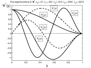
Figure 1. Five first real eigenfunctions of the operator (6.1) for $l=1$.

6.3. $\lambda_{0}(l)$ changes sign: numerical evidence

It is clear that, for large $l$, the non-symmetric perturbation $-\frac{1}{4}\,yD_{y}$ becomes essential in ${\bf B}^{*}$, and Sturm’s zero property in Figure 1 does not remain true. In Figure 2(a), (b), we present the shooting results of numerical calculating first three roots of the branch of the first eigenvalue $\{\lambda_{0}(l)\}$:

(6.11) $$\lambda_{0}(l)=0\,\,\,\mbox{at first three roots}\quad l_{1}=4.08...\,,\,\,\,l_{2}=7.25...\,,\,\,\,\mbox{and}\,\,\,l_{3}=10.\,...\,.$$

Note that $l_{1}$ is about $3\%$ close to the bound $l_{*}=3.9779...$ derived in (6.8). Further results of numerical experiments are shown in Table 1 fixing these 3–4 roots of $\lambda_{0}(l)$.

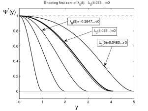
(a) first zero $l_{1}=4.08...$

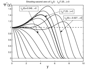
(b) second zero $l_{2}=7.25...$

Figure 2. Shooting zeros of $\lambda_{0}(l)$: first zero (a) and the second one (b).

Table 1. Some values of $\lambda_{0}(l)$

$l$	$\lambda_{0}(l)$
$1$	$-31.16...$
$2$	$-1.83...$
$3$	$-0.2647...$
$4$	$-0.008152...$
$4.075$	$-0.000236...$
$4.0775\approx l_{1}\quad$	$0.0000113...$
$4.08$	$0.00026...$
$4.1$	$0.0022...$
$4.2$	$0.011...$
$5$	$0.0483...$
$5$	$0.0483...$
$6$	$0.046...$
$7.25\approx l_{2}$	$0.00167...$
$7.5$	$-0.0097...$
$8$	$-0.027...$
$9$	$-0.018...$
$10\approx l_{3}$	$-0.00084...$
$11$	$0.00397...$
$12$	$0.00172...$
$13\approx l_{4}$	$-0.00055...$

Thus, taking into account these numerical results, in view of (6.2), we conclude that

(6.12) $$\framebox{$(0,0)\,\,\,\mbox{is regular for $l\in(0,l_{1})$, is irregular (singular) for $l\in[l_{1},l_{2}]$, etc.}$}$$

In addition, since $\lambda_{0}(l_{1})=0$, one can expect that for $l=l_{1}$, the vertex $(0,0)$ remains irregular, but now it is not singular, i.e., $u(0,0^{-})\not=0$ (under a natural non-orthogonality condition) is finite. Same happens for other roots $\lambda_{k}$ of $\lambda_{0}(l)$ (provided that the rest of eigenvalues are “ordered”, which has not been proved for arbitrary $l>0$).

6.4. Boundary layer and branching at $l=+\infty$

The phenomenon of the boundary layer (BL) occurring as $l\to\infty$ is explained by Figure 3. It follows that already at $l=20$, the first eigenfunction $\Psi_{0}^{*}(y)$ of ${\bf B}^{*}$ has a matching structure of the Boundary Layer for $y\approx l$ with the constant eigenfunction $\psi_{0}^{*}(y)\equiv 1$ (see (5.19)), which dominates for $l\leq 12$.

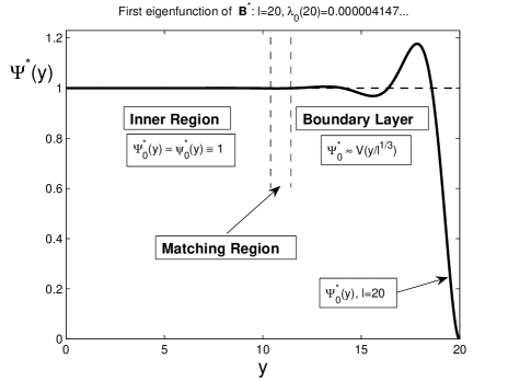
Figure 3. The boundary layer structure of $\Psi_{0}^{*}(y)$ for $l=20$.

The BL structure here is simple and standard; see more details in Section 7.2, where the BL is constructed for the parabolic PDE. Briefly, asymptotically sharp, in the BL for $y\sim l\gg 1$, equation (6.4) for $|\lambda_{0}(l)|\ll 1$ being asymptotically small (see (6.19)) reads

(6.13) $$\begin{matrix}-(\Psi^{*})^{(4)}-\frac{1}{4}\,l\,(\Psi^{*})^{\prime}+...=0\quad\Longrightarrow\quad\Psi^{*}=V(z)+...\,,\,\,\,z=l^{\frac{1}{3}}y,\quad\mbox{where}\quad\quad\vskip 3.0pt plus 1.0pt minus 1.0pt\vskip 3.0pt plus 1.0pt minus 1.0pt\\ -V^{(4)}-\frac{1}{4}\,V^{\prime}=0,\,\,\,z\in(0,l^{\frac{4}{3}});\,\,\,V=V^{\prime}=0,\,\,z=l^{\frac{4}{3}};\,\,\,V(0)=1.\qquad\qquad\qquad\end{matrix}$$

The BL-function $V$ is given explicitly (cf. (7.10)): denoting $b=2^{-5/3}$ and $a=\sqrt{3}\,b$,

(6.14) $$\begin{matrix}V(z)=C_{3}-{\mathrm{e}}^{-bz}\big{[}C_{1}\cos(az)+C_{2}\sin(az)\big{]},\,\,\,C_{1}=\frac{{\mathrm{e}}^{bl^{4/3}}[\cos(al^{4/3})-\frac{1}{\sqrt{3}}\,\sin(al^{4/3})]}{1-{\mathrm{e}}^{bl^{4/3}}[\cos(al^{4/3})-\frac{1}{\sqrt{3}}\,\sin(al^{4/3})]},\quad\vskip 3.0pt plus 1.0pt minus 1.0pt\\ C_{2}=\frac{{\mathrm{e}}^{bl^{4/3}}[\sin(al^{4/3})+\frac{1}{\sqrt{3}}\,\cos(al^{4/3})]}{1-{\mathrm{e}}^{bl^{4/3}}[\cos(al^{4/3})-\frac{1}{\sqrt{3}}\,\sin(al^{4/3})]},\quad C_{3}=\frac{1}{1-{\mathrm{e}}^{bl^{4/3}}[\cos(al^{4/3})-\frac{1}{\sqrt{3}}\,\sin(al^{4/3})]}.\quad\end{matrix}$$

The eigenvalue $\lambda_{0}(l)$ for $l\gg 1$ is then obtained by matching in $\mathbb{R}$: extending $\hat{\Psi}_{0}^{*}=\Psi_{0}^{*}H(l-y)$, where $H$ is the Heaviside function, we have (see Section 7.3 for details)

(6.15) $$\begin{matrix}(\hat{\Psi}_{0}^{*})^{(4)}(y)=(\Psi_{0}^{*})^{(4)}(y)H-(\Psi_{0}^{*})^{\prime\prime\prime}(l)\delta(y-l)-(\Psi_{0}^{*})^{\prime\prime}(l)\delta^{\prime}(y-l),\qquad\qquad\vskip 3.0pt plus 1.0pt minus 1.0pt\vskip 3.0pt plus 1.0pt minus 1.0pt\\ \mbox{where}\,\,\,(\Psi_{0}^{*})^{\prime\prime}(l)=l^{\frac{2}{3}}V^{\prime\prime}(l^{\frac{4}{3}})+...,\quad(\Psi_{0}^{*})^{\prime\prime\prime}(l)=l\,V^{\prime\prime\prime}(l^{\frac{4}{3}})+...\,.\qquad\qquad\quad\end{matrix}$$

Then (6.4) for $\lambda_{0}(l)$ reads

(6.16) $${\bf B}^{*}\hat{\Psi}^{*}-l\,V^{\prime\prime\prime}(l^{\frac{4}{3}})\delta(y-l)-l^{\frac{2}{3}}V^{\prime\prime}(l^{\frac{4}{3}})\delta^{\prime}(y-l)+...=\lambda_{0}(l)\hat{\Psi}_{0}^{*}\quad\mbox{in}\quad\mathbb{R}.$$

Finally, substituting $\hat{\Psi}_{0}^{*}=\psi_{0}^{*}+w\equiv 1+w$, where $w\bot\psi_{0}$, yields

(6.17) $${\bf B}^{*}w-l\,V^{\prime\prime\prime}(l^{\frac{4}{3}})\delta(y-l)-l^{\frac{2}{3}}V^{\prime\prime}(l^{\frac{4}{3}})\delta^{\prime}(y-l)+...=\lambda_{0}(l)+...\,.$$

Hence, by the orthogonality condition to $\psi_{0}(y)=F(y)$ (recall that ${\bf B}^{*}w\bot\psi_{0}$), (6.17) implies the following asymptotic expression for the eigenvalue:

(6.18) $$\begin{matrix}\lambda_{0}(l)=-\langle l\,V^{\prime\prime\prime}(l^{\frac{4}{3}})\delta(y-l)-l^{\frac{2}{3}}V^{\prime\prime}(l^{\frac{4}{3}})\delta^{\prime}(y-l),\psi_{0}\rangle+...\vskip 3.0pt plus 1.0pt minus 1.0pt\vskip 3.0pt plus 1.0pt minus 1.0pt\\ \equiv-l\,V^{\prime\prime\prime}(l^{\frac{4}{3}})\psi_{0}(l)+l^{\frac{2}{3}}V^{\prime\prime}(l^{\frac{4}{3}})\psi_{0}^{\prime}(l)+...\,.\qquad\quad\end{matrix}$$

Overall, using the asymptotics (5.12), (5.13) for the rescaled kernel and taking into account (6.14), we obtain from (6.18) the following typical approximate oscillatory behaviour:

(6.19) $$\textstyle{\lambda_{0}(l)\sim l^{\frac{2}{3}}{\mathrm{e}}^{-\hat{d}_{0}\,l^{4/3}}\cos\big{(}\hat{b}_{0}\,l^{\frac{4}{3}}\big{)}\quad\mbox{for}\quad l\gg 1,\quad\hat{d}_{0}\sim d_{0}+b,\,\,\hat{b}_{0}\sim\frac{b_{0}+a}{2},}$$

where we omit constants. In fact, (6.19) shows how an $l$-branch of the first eigenvalue $\lambda_{0}(l)$ bifurcates at $l=+\infty$ from $\lambda_{0}(\infty)=0$ for the operator ${\bf B}^{*}$ with the spectrum (5.15), $m=2$. It is not that difficult to show that similar branching occurs from any eigenvalue

(6.20) $$\textstyle{\lambda_{k}=-\frac{k}{4}\quad\mbox{for}\quad k=0,1,2,...\quad\Longrightarrow\quad\exists\,\,\,\lambda_{k}(l)\quad\mbox{for}\quad l\gg 1,\,\,\,\lambda_{k}(\infty)=-\frac{k}{4},}$$

where (6.19) is evidently the only eigenvalue that can change sign. The branching happens in the framework of classic perturbation theory for linear operators (see Kato [39]), so we do not treat this any further. Actually, the branching (6.20) or (6.10) is the only for us reason for the operator (6.1) to admit many real eigenvalues for various values of $l>0$.

7. Bi-harmonic PDE for $m=2$: Blow-up asymptotic derivation of Petrovskii-type regularity criterion by eigenfunction expansion

Regardless nonexistence of a definite answer concerning regularity of the vertex of the fundamental parabolae (4.13), nevertheless, we next show that there is a way to move towards a Petrovskii-like criterion for the case of more expanding lateral boundaries for functions (4.7). However, the results in Section 6 (treated according to the limit $l=l(\tau)\to+\infty$) imply, in view of the oscillatory behaviour of the first eigenvalue in (6.19), that a direct regularity conclusion for a given $\varphi(\tau)$ is not possible in principle. To get the regular vertex $(0,0)$, a procedure of oscillatory cut off of the boundary must be performed.

At this moment, in Appendix A, we continue our study with a certain brief, rather questionable, and even controversial suggestion, which nevertheless is quite attractive and actually goes along the lines of Petrovskii’s barrier ideas, so we fairly believe this is a right (and unique) place for such a discussion.

As a next step, we return to the spectral methods that cover both regular/irregular issues for (4.1), which indeed are more complicated than for the heat equation (3.1).

7.1. Two-region expansion

Thus, we return to the rescaled problem (4.12) for $m=2$. As usual in any matching asymptotic analysis, this blow-up problem is solved by matching of expansions in two regions:

(i) Inner Region, which is situated around the origin $y=0$, and

(ii) Boundary Region close to the boundaries $y=\pm\varphi(\tau)$, where a boundary layer occurs.

Actually, such a two-region structure, with the asymptotics specified below, defines the class of generic solutions under consideration according to (4.3) (those in (4.4) are all different). We begin with the simpler analysis in the Boundary Region (ii).

7.2. Boundary Layer (BL) structure

Sufficiently close to the lateral boundary of $Q_{0}$, it is natural to introduces the variables

(7.1) $$\textstyle{z=\frac{y}{\varphi(\tau)}\quad\mbox{and}\quad v(y,\tau)=w(z,\tau)\quad\Longrightarrow\quad w_{\tau}=-\frac{1}{\varphi^{4}}\,w_{zzzz}-\frac{1}{4}\,zw_{z}+\frac{\varphi^{\prime}}{\varphi}\,zw_{z}.}$$

We next introduce the BL-variables

(7.2) $$\textstyle{\xi=\varphi^{\frac{4}{3}}(\tau)(1-z),\quad\varphi^{\frac{4}{3}}(\tau){\mathrm{d}}\tau={\mathrm{d}}s,\quad\mbox{and}\quad w(z,\tau)=\rho(s)g(\xi,s),}$$

where $\rho(s)$ is an unknown slow decaying (in the same natural sense, associated with (4.8)) time-factor depending on the function $\varphi(\tau)$, e.g., $\sim\frac{1}{\varphi(\tau)}$ as a clue. On substitution into the PDE in (7.1), we obtain the following perturbed equation:

(7.3) $$\begin{matrix}g_{s}={\bf A}g-\frac{1}{4}\,\varphi^{-\frac{4}{3}}\xi g_{\xi}-\frac{\varphi^{\prime}_{\tau}}{\varphi}\,\big{(}1-\xi\varphi^{-\frac{4}{3}}\big{)}g_{\xi}\vskip 3.0pt plus 1.0pt minus 1.0pt\vskip 3.0pt plus 1.0pt minus 1.0pt\\ -\frac{4}{3}\,\varphi^{-\frac{1}{3}}\varphi^{\prime}_{\tau}\xi g_{\xi}-\frac{\rho^{\prime}_{s}}{\rho}\,g,\quad\mbox{where}\quad{\bf A}g=-g^{(4)}+\frac{1}{4}\,g^{\prime}.\end{matrix}$$

As usual in boundary layer theory, following (4.3), we are looking for a generic pattern of the behaviour described by (7.3) on compact subsets near the lateral boundary,

(7.4) $$|\xi|=o\big{(}\varphi^{-\frac{4}{3}}(\tau)\big{)}\quad\Longrightarrow\quad|z-1|=o\big{(}\varphi^{-\frac{8}{3}}(\tau)\big{)}\quad\mbox{as}\quad\tau\to+\infty.$$

On these space-time compact subsets, the second term on the right-hand side of (7.3) becomes asymptotically small, while all the others are much smaller in view of the slow growth/decay assumptions such as (4.8) for $\varphi(\tau)$ and $\rho(s)$.

Then posing the asymptotic behaviour at infinity:

(7.5) $$g(\xi,s)\to 1\quad\mbox{as}\quad\xi\to+\infty\quad(\mbox{Hypothesis I for generic patterns}),$$

where all the derivatives are assumed to vanish, we arrive at the problem of passing to the limit as $s\to+\infty$ in the problem (7.3), (7.5). Assuming that, by the definition in (7.2), the rescaled orbit $\{g(s),\,\,s>0\}$ is uniformly bounded, by classic parabolic theory [19], one can pass to the limit in (7.3) along a sequence $\{s_{k}\}\to+\infty$. Namely, by the above, we have that, uniformly on compact subsets defined in (7.4), as $k\to\infty$,

(7.6) $$g(s_{k}+s)\to h(s),\quad\mbox{where}\quad h_{s}={\bf A}h,\quad h=h_{\xi}=0\,\,\,\mbox{at}\,\,\,\xi=0,\quad h|_{\xi=+\infty}=1.$$

The limit (at $s=+\infty$) equation obtained from (7.3):

(7.7) $$\textstyle{h_{s}={\bf A}h\equiv-h_{\xi\xi\xi\xi}+\frac{1}{4}\,h_{\xi}}$$

is a standard linear parabolic PDE in the unbounded domain $\mathbb{R}_{+}$, though it is governed by a non self-adjoint operator ${\bf A}$. We need to show that, in an appropriate weighted $L^{2}$-space if necessary, under the hypothesis (7.5), the stabilization holds, i.e., the $\omega$-limit set of $\{h(s)\}$ consists of equilibria: as $s\to+\infty$,

(7.8) $$\left\{\begin{matrix}h(\xi,s)\to g_{0}(\xi),\quad\mbox{where}\quad{\bf A}g_{0}=0\,\,\,\mbox{for}\,\,\,\xi>0,\vskip 3.0pt plus 1.0pt minus 1.0pt\vskip 3.0pt plus 1.0pt minus 1.0pt\\ g_{0}=g_{0}^{\prime}=0\quad\mbox{for}\quad\xi=0,\quad g_{0}(+\infty)=1.\qquad\,\,\end{matrix}\right.$$

The characteristic equation for the linear operator ${\bf A}$ yields

(7.9) $$\textstyle{-\lambda^{4}+\frac{1}{4}\,\lambda=0\quad\Longrightarrow\quad\lambda_{1}=0\quad\mbox{and}\quad\lambda_{2,3}=\frac{1}{4^{1/3}}\big{(}-\frac{1}{2}\pm{\rm i}\,\frac{\sqrt{3}}{2}\big{)}.}$$

This gives the unique solution of (7.8), shown in Figure 4,

(7.10) $$\textstyle{g_{0}(\xi)=1-{\mathrm{e}}^{-\frac{\xi}{2^{5/3}}}\,\big{[}\cos\big{(}\frac{\sqrt{3}\,\xi}{2^{5/3}}\big{)}+\frac{1}{\sqrt{3}}\,\sin\big{(}\frac{\sqrt{3}\,\xi}{2^{5/3}}\big{)}\big{]}.}$$

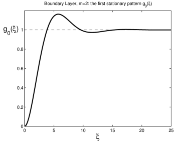
Figure 4. The unique stationary solution $g_{0}(\xi)$ of the problem (7.8).

We do not concentrate on this stabilization problem (7.8), which reduces to a standard spectral study of ${\bf A}$ in a weighted space. Let us mention that, in the metric of $L^{2}(\mathbb{R}_{+})$, the operator has a clear exponential stability feature. Consider the eigenvalue problem

(7.11) $$\textstyle{{\bf A}\psi\equiv-\psi^{(4)}+\frac{1}{4}\,\psi^{\prime}=\lambda\psi.}$$

As customary, multiplying this by $\bar{\psi}$, next taking the complex conjugate of the equation and multiplying by $\psi$ and summing up the resulting equalities yields

(7.12) $$\textstyle{(\lambda+\bar{\lambda})\int|\psi|^{2}=-2\int|\psi^{\prime\prime}|^{2}+\frac{1}{4}\int(\bar{\psi}\psi^{\prime}+\psi\bar{\psi}^{\prime})\equiv-2\int|\psi^{\prime\prime}|^{2}<0,}$$

i.e., ${\rm Re}\,\lambda<0$ for any $\lambda\in\sigma({\bf A})$ (this does not take into account a continuous spectrum).

Actually, the convergence (7.6) and (7.8) for the perturbed dynamical system (7.3) is the main Hypothesis (H), which characterizes the class of generic patterns under consideration, and then (7.5) is its partial consequence. Note that the uniform stability of the stationary point $g_{0}$ in the limit autonomous system (7.7) in a suitable metric will guarantee that the asymptotically small perturbations do not affect the omega-limit set; see [33, Ch. 1].

We stop further discussion concerning the passage to the limit in (7.3) and summarize the conclusions as follows:

Proposition 7.1.

Under the given hypothesis and conditions, the problem $\eqref{z3}$ admits a family of solutions (called generic) that satisfy $\eqref{z10}$.

We must admit that such a definition of generic patterns looks rather non-constructive, which is unavoidable for higher-order parabolic PDEs without positivity issues. Note that, according to (3.14), a similar obscure issue appears even for the heat equation in (3.1). One can expect that (7.8) occurs for “almost all” solutions, excluding just those that have eventually the faster vanishing first Fourier coefficient that some others. Then another BL is needed, but we do not intent to describe an invariant manifold structure of such a thin solution set (recall that (7.3) is a difficult non-autonomous PDE).

7.3. Inner Region analysis: towards the regularity criterion

In Inner Region, we deal with the original rescaled problem (4.12). Without loss of generality, for simplicity of key calculations, we consider symmetric solutions defined for $y>0$ by assuming the symmetry conditions:

(7.13) $$v_{y}=v_{yyy}=0\quad\mbox{at\,\,\, $y=0$}.$$

In order to apply the standard eigenfunction expansion techniques by using the orthonormal set of polynomial eigenfunctions of ${\bf B}^{*}$ given in (5.19), as customary in classic PDE theory, we extend $v(y,\tau)$ by 0 for $y>\varphi(\tau)$:

(7.14) $$\hat{v}(y,\tau)=v(y,\tau)H(\varphi(\tau)-y)=\left\{\begin{matrix}v(y,\tau)\quad\mbox{for}\quad 0\leq y<\varphi(\tau),\\ \,\,0\,\,\quad\mbox{for}\quad\,\,y\geq\varphi(\tau),\end{matrix}\right.$$

where $H$ is the Heaviside function. Since $v=v_{y}=0$ on the lateral boundary $\{y=\varphi(\tau)\}$, one can check that, in the sense of distributions,

(7.15) $$\begin{matrix}\hat{v}_{\tau}=v_{\tau}H,\quad\hat{v}_{y}=v_{y}H,\quad\hat{v}_{yy}=v_{yy}H,\vskip 3.0pt plus 1.0pt minus 1.0pt\vskip 3.0pt plus 1.0pt minus 1.0pt\\ \hat{v}_{yyy}=v_{yyy}H-v_{yy}\big{|}_{y=\varphi}\delta(y-\varphi),\vskip 3.0pt plus 1.0pt minus 1.0pt\vskip 3.0pt plus 1.0pt minus 1.0pt\\ \hat{v}_{yyyy}=v_{yyyy}H-v_{yyy}\big{|}_{y=\varphi}\delta(y-\varphi)-v_{yy}\big{|}_{y=\varphi}\delta^{\prime}(y-\varphi).\end{matrix}$$

Therefore, $\hat{v}$ satisfies the following equation:

(7.16) $$\hat{v}_{\tau}={\bf B}^{*}\hat{v}-v_{yyy}\big{|}_{y=\varphi}\delta(y-\varphi)-v_{yy}\big{|}_{y=\varphi}\delta^{\prime}(y-\varphi)\quad\mbox{in}\quad\mathbb{R}_{+}\times\mathbb{R}_{+}.$$

Since, obviously, the extended solution orbit (7.14) is uniformly bounded in $L^{2}_{\rho^{*}}(\mathbb{R})$, we can use the converging in the mean (and uniformly on compact subsets in $y$) the eigenfunction expansion via the generalized Hermite polynomials (5.19):

(7.17) $$\textstyle{\hat{v}(y,\tau)=\sum\limits_{(k\geq 0)}a_{k}(\tau)\psi_{k}^{*}(y).}$$

Substituting (7.17) into (7.16) and using the orthonormality property (5.20) yields the following dynamical system for the expansion coefficients: for all $k=0,1,2,...\,,$

(7.18) $$\textstyle{a_{k}^{\prime}=\lambda_{k}a_{k}-v_{yyy}\big{|}_{y=\varphi(\tau)}\langle\delta(y-\varphi(\tau)),\psi_{k}\rangle-v_{yy}\big{|}_{y=\varphi(\tau)}\langle\delta^{\prime}(y-\varphi),\psi_{k}\rangle,}$$

where $\lambda_{k}=-\frac{k}{4}$ are real eigenvalues (5.15). Recall that $\lambda_{k}<0$ for all $k\geq 1$. More importantly, the corresponding eigenfunctions $\psi_{k}(y)$ are unbounded and not monotone for $k\geq 1$ according to (5.21). Therefore, regardless proper asymptotics given by (7.18), these inner patterns cannot be matched with the BL-behaviour such as (7.5), and demand other matching theory (since these are not generic, the latter is not developed).

Thus, bearing again in mind (4.3), one needs to concentrate on the “maximal” first Fourier generic pattern associated with

(7.19) $$k=0:\quad\lambda_{0}=0\quad\mbox{and}\quad\psi_{0}^{*}(y)\equiv 1\quad\big{(}\psi_{0}(y)=F(y)\big{)}.$$

Actually, this corresponds to the centre subspace behaviour for the equation (7.18):

(7.20) $$\hat{v}(y,\tau)=a_{0}(\tau)+w^{\bot}(y,\tau),\quad\mbox{where}\quad w^{\bot}\in{\rm Span}\{\psi_{k}^{*},\,\,k\geq 1\},$$

and $w^{\bot}(y,\tau)$ is then negligible relative to $a_{0}(\tau)$. This is another characterization of our class of generic patterns, Hypothesis II. The equation for $a_{0}(\tau)$ then takes the form:

(7.21) $$\textstyle{a_{0}^{\prime}=-v_{yyy}\big{|}_{y=\varphi(\tau)}\psi_{0}(\varphi(\tau))+v_{yy}\big{|}_{y=\varphi(\tau)}\psi^{\prime}_{0}(\varphi(\tau)).}$$

We now return to BL theory established the boundary behaviour (7.2) for $\tau\gg 1$, which for convenience we state again: in the rescaled sense, on the given compact subsets,

(7.22) $$\textstyle{v(y,\tau)=\rho(s)g_{0}\big{(}\varphi^{\frac{4}{3}}(\tau)(1-\frac{y}{\varphi(\tau)})\big{)}+...\,.}$$

By the matching of both Regions, one concludes that, for such generic patterns,

(7.23) $$\textstyle{\frac{a_{0}(\tau)}{\rho(s)}\to 1\quad\mbox{as}\quad\tau\to\infty\quad\Longrightarrow\quad\rho(s)=a_{0}(\tau)(1+o(1)).}$$

Then the convergence (7.22), which by regularity is also true for the spatial derivatives, yields, in the natural rescaled sense,

(7.24) $$\begin{matrix}v_{yy}\big{|}_{y=\varphi(\tau)}\to\rho(s)\varphi^{\frac{2}{3}}(\tau)\gamma_{1}\to a_{0}(\tau)\varphi^{\frac{2}{3}}(\tau)\gamma_{1},\quad\gamma_{1}=g_{0}^{\prime\prime}(0)>0,\vskip 3.0pt plus 1.0pt minus 1.0pt\vskip 3.0pt plus 1.0pt minus 1.0pt\\ v_{yyy}\big{|}_{y=\varphi(\tau)}\to-\rho(s)\varphi(\tau)\gamma_{2}\to-a_{0}(\tau)\varphi(\tau)\gamma_{2},\quad\gamma_{2}=g_{0}^{\prime\prime\prime}(0).\end{matrix}$$

Eventually, this leads to the following asymptotic ODE for the first expansion coefficient for generic patterns:

(7.25) $$\textstyle{\frac{a_{0}^{\prime}}{a_{0}}=G_{2}(\varphi(\tau))\equiv\gamma_{2}\varphi(\tau)\psi_{0}(\varphi(\tau))+\gamma_{1}\varphi^{\frac{2}{3}}(\tau)\psi_{0}^{\prime}(\varphi(\tau))+...\quad\mbox{for}\quad\tau\gg 1.}$$

For instance, this gives a first easy condition of regularity of $(0,0)$: for the generic patterns, this is the “negative” divergence of the following integral:

(7.26) $$\textstyle{\int\limits^{\infty}G_{2}(\varphi(\tau))\,{\mathrm{d}}\tau\quad\mbox{diverges to $-\infty$}\quad\Longrightarrow\quad a_{0}(\tau)\to 0\quad\mbox{as}\quad\tau\to+\infty.}$$

In order to obtain more practical and sufficiently sharp conditions of regularity, we will use the expansion (5.12) of the first eigenfunction $\psi_{0}(y)=F(y)$, which on substitution into the right-hand side in (7.25), where both terms are equivalent, yields

(7.27) $$\textstyle{\frac{a_{0}^{\prime}}{a_{0}}=\hat{\gamma}\varphi^{\frac{2}{3}}(\tau)C_{3}\cos\big{(}b_{0}\varphi^{\frac{4}{3}}(\tau)+C_{4}\big{)}{\mathrm{e}}^{-d_{0}\varphi^{4/3}(\tau)}+...\quad\mbox{for}\quad\tau\gg 1,}$$

with some $\hat{\gamma}\not=0$ and constants $C_{3,4}$ depending in an obvious way on $C_{1,2}$ in (5.12) and other parameters from (5.13). Integrating implies that

(7.28) $$\textstyle{\ln|{a_{0}(\tau)}|=\hat{\gamma}\int\limits^{\tau}\varphi^{\frac{2}{3}}(s)C_{1}\cos\big{(}b_{0}\varphi^{\frac{4}{3}}(s)+C_{2}\big{)}{\mathrm{e}}^{-d_{0}\varphi^{4/3}(s)}\,{\mathrm{d}}s+...\quad\mbox{for}\quad\tau\gg 1.}$$

Irregularity condition. This is straightforward: (7.28) implies that the limit of $a_{0}(\tau)$ as $\tau\to+\infty$ can be arbitrary (i.e., not necessarily zero), if the integral converges. Therefore, up to the achieved accuracy of the expansions and matching, we state the following condition of the irregularity of $(0,0)$ (all the irrelevant constants are omitted):

(7.29) $$\framebox{$(0,0)\quad\mbox{is irregular if}\quad\int\limits^{\infty}\varphi^{\frac{2}{3}}(s)\cos\big{(}b_{0}\varphi^{\frac{4}{3}}(s)\big{)}\,{\mathrm{e}}^{-d_{0}\varphi^{4/3}(s)}\,{\mathrm{d}}s\quad\mbox{converges}.$}$$

Then, obviously, $u(0,0^{-})\not=0$ (a natural non-orthogonality condition required) is finite, i.e., the vertex $(0,0)$ is irregular, but non-singular. This still looks pretty similar to Petrovskii’s criterion in (3.11).

Regularity condition: oscillatory cut-off of $\varphi(\tau)$. Thus, assume that $\varphi(\tau)$ is close to the desired (and still unknown) critical irregularity/regularity situation, and that we follow the first Fourier coefficient equation (7.27) or (7.28), within the given accuracy. Then, for using (7.28) for the purpose of the regularity analysis, we observe that the presence in the integral the oscillatory factor can always $\cos(\cdot)$ violate the (uniform) divergence to $-\infty$ hypothesis in (7.26). Indeed, then $\ln|a_{0}(\tau)|\to\pm\infty$ along different subsequences $\{\tau=\tau_{k}^{\pm}\}\to+\infty$, and the limit to $+\infty$ does not guarantee (7.26) (of course, for such limits, our matching with the BL can be violated as well, but we do not discuss this issue here). In other words, in the case of oscillatory kernels, a pure divergence of the integral in (7.28) does not guarantee the point regularity. This is the principal difference with the positive kernel case; cf. (7.36) below with no oscillatory component in the integral. Let us note that, in general, the standard divergence of (7.28) will ensure that that the vertex $(0,0^{-})$ is irregular and is also singular in the sense of (4.15). Moreover, $u(x,t)$ has infinite oscillatory behaviour as $(x,t)\to(0,0^{-})$, i.e., eventually oscillations get both $\pm\infty$.

Thus, under the accepted hypothesis, the oscillatory part of the rescaled fundamental kernel (5.12) of the operator under consideration can violate the regularity of boundary point for any slow growing factor $\varphi(\tau)$ satisfying (4.7)–(4.9), even if the integral diverges. As we have seen in Section 6, for higher-order operators, the regularity condition “above” the fundamental parabolae (4.13) becomes rather subtle and sensitive. Indeed, according to the integral in (7.28), arbitrarily small perturbations of $\varphi(\tau)$ can “switch over” regularity to the irregularity and vice versa.

To guarantee regularity, an extra “oscillatory cut-off” of $\varphi(\tau)$ is then necessary to be introduced after a necessary remark.

7.4. Remark 1: an analogy with elliptic theory

This principal difficulty concerning the kernels of changing sign has a known counterpart in regularity elliptic theory for (2.1). Namely, it was first shown in [70] (1986) for $m=2$, $N\geq 8$ that the vertex of a cone can be irregular (singular) if the fundamental solution of $L(\partial)$ for $N>2m$

(7.30) $$\textstyle{F(x)=\Psi\big{(}\frac{x}{|x|}\big{)}|x|^{2m-N},\quad x\in\mathbb{R}^{N}\setminus\{0\}\quad(N>2m)}$$

changes sign; see further comments and references in [68, § 1]. Then in elliptic theory, the regularity analysis is performed for a restricted subclass of operators $L(\partial)$ called positive with weight $F$. This actually means that $F>0$ [68, § 3] (cf. a positivity-like condition in [27] for $m=2$ and [21]), so, until now, refined elliptic regularity results for kernels of essentially (e.g., infinitely many) changing sign seem be unavailable. As in classic theory [49, 71], this analysis demands constructing corresponding generalized Hermite polynomials as eigenfunctions of an adjoint pencil of linear operators along the lines of those obtained for hyperbolic equations; see [32, p. 254] and [29] (for $u_{tt}=-u_{xxxx}$; see the end of Section 8 below). The oscillatory cut-off of the boundary will then be essential. An example of such an elliptic evolution approach for studying singularities of (2.2) in $\mathbb{R}^{2}$, $q\in(0,1)$ (with many additional references presented) is given in [10].

Of course, it is well-known and this is a classic matter, that general theory of operator pencils associated with corner singularities has been well-developed for a number of elliptic equations; see [52, 53] and [27] for references to other papers and related monographs and as a source of further extensions to be traced out by the MathSciNet. For other types of parabolic or elliptic problems mentioned above, new operator pencils appear. In the parabolic case, we do not intend to change the operator $-D_{x}^{4}$ in related lines, but then need instead to perform a refined oscillatory cut-off of the lateral boundary.

7.5. Optimal regularity conditions for generic patterns

Thus, to guarantee the regularity, we perform the procedure of oscillatory cut-off of a given function $\varphi(\tau)$. Namely, this means that a smooth $\widetilde{\varphi}(\tau)$ replaces $\varphi(\tau)$, for which

(7.31) $$\textstyle{\hat{\gamma}C_{1}\cos\big{(}b_{0}\widetilde{\varphi}^{\frac{4}{3}}(\tau)+C_{2}\big{)}\approx\big{[}\hat{\gamma}C_{1}\cos\big{(}b_{0}\varphi^{\frac{4}{3}}(\tau)+C_{2}\big{)}\big{]}_{-}}$$

asymptotically sharp up to absolutely convergent perturbations in the integral (7.28), where $[\cdot]_{-}$ denotes the negative part. This is necessary to cut-off the positive part of the diverging integral. Figure 5 schematically explains how (7.31) works (for $\hat{\gamma}C_{1}>0$) by cutting off all positive waves of the $\cos$-function for $\tau\gg 1$ and creating “almost discontinuous” (jumping-like) $\widetilde{\varphi}(\tau)$, which in the figure is denoted by $\varphi_{\rm cut}(\tau)$. Using necessary smoothing at the points, where $\cos(\cdot)$ changes sign, for any such monotone increasing $\varphi(\tau)$, the corresponding $\widetilde{\varphi}(\tau)$ can be also chosen increasing. In other words, the resulting $\widetilde{\varphi}(\tau)$ sufficiently fast jumps over those intervals of the length $l$, which in Section 6 were determined as leading to the irregular vertex. We do not pay special attention to the question on how such smoothly jumping boundary can affect the boundary layer behaviour described by the equation (7.3), where the term $\varphi^{\prime}/\varphi$ may then play a role (fortunately, not dominant). However, it is clear that, since the correct intervals of the behaviour of $\widetilde{\varphi}(\tau)$ get arbitrarily long as $\tau\to\infty$, we have enough time for establishing the BL-structure, so that formulae (8.5) remain true closer to the end of each of them, and further analysis applies. In addition, it is also clear that, once the solution gets very small by (7.25) at the end of a fixed such interval in $\tau$, a smooth monotone increasing jump of $\widetilde{\varphi}(\tau)$ at the end point cannot essentially affect the value of the solution during such a short interval of time. This means that, on the next good interval, the solution remains small and continues to be governed by the eigenspace ${\rm Span}\,\{\psi_{0}^{*}\}$.

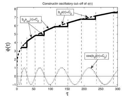
Figure 5. A schematic view of a proper oscillatory cut-off of $\varphi(\tau)$.

Thus, according to the oscillatory cut-off (7.31), the condition of regularity is as follows:

(7.32) $$\framebox{$(0,0)\quad\mbox{is regular if}\quad\int\limits^{\infty}\widetilde{\varphi}^{\frac{2}{3}}(s)\cos\big{(}b_{0}\widetilde{\varphi}^{\frac{4}{3}}(s)+C_{2}\big{)}\,{\mathrm{e}}^{-d_{0}\widetilde{\varphi}^{4/3}(s)}\,{\mathrm{d}}s\quad\mbox{diverges}.$}$$

There is a clear gap between the irregularity (7.29) and the regularity (7.32) conditions, so that an Osgood–Dini-like criterion cannot be available in principle.

With such a procedure, similar to Petrovskii’s presentation (3.9) of the boundary regularity results, we deduce that:

(7.33) $$\framebox{$\begin{matrix}{\rm(i)}\,\,\widetilde{R}(t)=3^{-\frac{3}{4}}\,2^{\frac{11}{4}}\,(-t)^{\frac{1}{4}}\,\big{[}\ln|\ln(-t)|\big{]}^{\frac{3}{4}}\,\Longrightarrow\,(0,0)\quad\mbox{is regular},\quad\mbox{and}\qquad\quad\vskip 3.0pt plus 1.0pt minus 1.0pt\vskip 3.0pt plus 1.0pt minus 1.0pt\\ {\rm(ii)}\,\,R(t)=\big{(}3^{-\frac{3}{4}}\,2^{\frac{11}{4}}+\varepsilon\big{)}\,(-t)^{\frac{1}{4}}\,\big{[}\ln|\ln(-t)|\big{]}^{\frac{3}{4}},\,\,\varepsilon>0\,\Longrightarrow\,(0,0)\quad\mbox{is irregular},\end{matrix}$}$$

where, in the regular $\widetilde{R}(t)$, the oscillatory cut-off meaning (7.31) must be assumed.

7.6. Remark 2: on other asymptotic patterns and related regularity

It follows from the dynamical system (7.18), that, in general, there exist other (non-generic) asymptotic patterns corresponding to the behaviour on each of a 1D stable eigenspace of ${\bf B}^{*}$, which hence are not governed by the expansion (7.20). Such a behaviour then will generate its own regularity/irregularity conditions with or without cut-offs of the corresponding similar integrals. Indeed, those asymptotic patterns will demand a different “BL-like” theory, for which (7.5) is not true. Since these are not generic and belong to the subspace of co-dimension one, a correct posing of the IBVP in $Q_{0}$ for such regular solutions is quite tricky and demands a priori unknown and non-constructive conditions on initial data $u_{0}$, so we have no reasons to take those into account. On the other hand, describing countable sets of various blow-up singularities is a serious problem of modern PDE theory, but currently this has a little to do with the boundary regularity analysis.

7.7. Remark 3: for the heat equation, the spectral–BL blow-up approach is sharp

Let us very briefly repeat and list the main steps of the above blow-up analysis for the classic problem (3.1) to prove (4.5). Thus, (4.6) reads

$$R(t)=(-t)^{\frac{1}{2}}\varphi(\tau),$$

where, in (4.12), we get the classic Hermite operator [11, p. 48]

$$\textstyle{{\bf B}^{*}=D_{y}^{2}-\frac{1}{2}\,yD_{y}\quad\mbox{in}\quad L^{2}_{\rho^{*}}(\mathbb{R}),\quad\rho^{*}(y)={\mathrm{e}}^{-\frac{y^{2}}{4}},\quad\sigma({\bf B}^{*})=\big{\{}\lambda_{k}=-\frac{k}{2},\,\,k=0,1,2,...\big{\}},}$$

with ${\mathcal{D}}({\bf B}^{*})=H^{2}_{\rho^{*}}(\mathbb{R})$, etc. Similar to (7.2), the BL variables and asymptotics are now

(7.34) $$\begin{matrix}\xi=\varphi^{2}(1-z)\equiv\varphi(\varphi-y)\quad\mbox{and}\quad w(z,\tau)=a_{0}(\tau)g(\xi,\tau)+...\,,\qquad\quad\vskip 3.0pt plus 1.0pt minus 1.0pt\vskip 3.0pt plus 1.0pt minus 1.0pt\vskip 3.0pt plus 1.0pt minus 1.0pt\\ \mbox{where}\,\,g(\xi,\tau)\to g_{0}(\xi),\,\,\,\tau\to\infty\,\,\mbox{and}\,\,g_{0}(\xi)=1-{\mathrm{e}}^{-\xi/2}\,\,\big{(}g_{0}^{\prime\prime}+\frac{1}{2}\,g_{0}^{\prime}=0\big{)}.\qquad\quad\end{matrix}$$

Using two formulae in the first line in (7.15) with

$$\hat{v}_{yy}=v_{yy}H-v_{y}\big{|}_{y=\varphi}\delta(y-\varphi),$$

we arrive at the equation (the analogy of (7.16))

$$\hat{v}_{\tau}={\bf B}^{*}\hat{v}+v_{y}\big{|}_{y=\varphi}\delta(y-\varphi).$$

Hence, asymptotically via the BL structure (7.34), for the generic patterns as usual, the analogy of (8.6) takes much simpler form:

(7.35) $$\textstyle{\frac{a_{0}^{\prime}}{a_{0}}=-\gamma_{1}\varphi\,\psi_{0}(\varphi)+...\quad\Longrightarrow\quad\frac{a_{0}^{\prime}}{a_{0}}=-\frac{\gamma_{1}}{2\sqrt{\pi}}\,\varphi\,{\mathrm{e}}^{-\frac{\varphi^{2}}{4}}+...\,,}$$

where $\gamma_{1}=g_{0}^{\prime}(0)=\frac{1}{2}$ and $\psi_{0}(y)=F(y)=\frac{1}{2\sqrt{\pi}}\,{\mathrm{e}}^{-y^{2}/4}$ is the positive rescaled Gaussian kernel of the heat operator. Thus, (7.35) justifies that, for the generic patterns, the regularity criterion reads

(7.36) $$\framebox{$\mbox{$(0,0)$ is regular iff}\quad\int\limits^{\infty}\varphi(\tau)\,{\mathrm{e}}^{-\frac{\varphi^{2}(\tau)}{4}}\,{\mathrm{d}}\tau=+\infty$}$$

(no cut-off is necessary in this non-oscillatory case). One can see that (7.36) is equivalent to that in (3.11) or (3.12). Recall that there exist other asymptotic patterns related to the stable subspace of ${\bf B}^{*}$ of co-dimension 1, which, as usual, is not taken into account.

8. On extensions to $2m$th-order poly-harmonic and other operators

We discuss the extensions of the asymptotic method to other PDEs.

8.1. Poly-harmonic equation

For (1.4), the spectral properties of the operator

(8.1) $$\textstyle{{\bf B}^{*}=-(-\Delta)^{m}-\frac{1}{2m}\,y\cdot\nabla}$$

are given in [17]. A sharp asymptotic expansion (similar to (5.12)) of the radially symmetric rescaled kernel $F(|y|)$ satisfying

(8.2) $$\textstyle{{\bf B}F=0\quad\mbox{in}\quad\mathbb{R}^{N},\quad\int F=1\quad\Longrightarrow\quad\psi_{\beta}(y)=\frac{(-1)^{|\beta|}}{\sqrt{\beta!}}\,D^{\beta}F(y),\,\,\,|\beta|=0,1,2,...\,,}$$

where $\beta$ is a multiindex in $\mathbb{R}^{N}$, is also not that difficult to get. Then (8.2) implies that the adjoint basis $\{\psi_{\beta}^{*}\}$ consists of generalized Hermite polynomials.

In the radial case, the critical $R(t)$ for boundary regularity is about

(8.3) $$R(t)=C_{*}\,(-t)^{\frac{1}{2m}}\,\big{[}\,\ln|\ln(-t)|\,\big{]}^{\frac{2m-1}{2m}},\quad\mbox{where}\quad C_{*}=d_{0}^{-\frac{1}{\alpha}}>0\,\,\,\mbox{is a constant},$$

and the oscillatory cut-off is assumed for the regularity. As usual, replacing $C_{*}$ by $C_{*}+\varepsilon$ for any $\varepsilon>0$ makes $(0,0)$ irregular.

Some calculations become more involved, especially in the case of non-radial $Q_{0}$, where the spatial shape of the shrinking cusp will affect the right-hand side of (7.27), where the BL structure, though having similar variables such as (7.2), is now governed by complicated elliptic problems instead of the ODE (7.11). For instance, if the boundary of $Q_{0}$ is given by the characteristic fundamental paraboloid in the $x$ and $y$ variables, respectively (i.e., $\varphi(\tau)\equiv 1$):

(8.4) $$\textstyle{\sum_{(|\alpha|=2m)}a_{\alpha}x^{\alpha}=(-t)\quad\Longrightarrow\quad\sum_{(|\alpha|=2m)}a_{\alpha}y^{\alpha}=1.}$$

The case $a_{\alpha}>0$ for any $\alpha$ corresponds to Miha${\rm\check{i}}$lov’s [72, 73, 74] and Kondrat’ev’s [48] cases. Hence, the regularity in the strong sense of the vertex $(0,0)$ depends on the spectrum of the operator (8.1) in the domain $I_{a}$ with the boundary given by (8.4). Similar to the analysis in Section 6, we have that, by Poincare’s inequality, $(0,0)$ is regular if the diameter of $I_{a}$ is not that large (since the eigenvalues of ${\bf B}^{*}$ are close to those for $-(-\Delta)^{m}<0$). On the contrary, since ${\bf B}^{*}$ is not self-adjoint and sign-definite, there are coefficients $\{a_{\alpha}>0\}$, for which the vertex $(0,0)$ is not regular in the classic sense.

If some of the coefficients $\{a_{\alpha}\}$ are negative (this is Fe${\rm\check{i}}$gin’s case [25]), ${\bf B}^{*}$ is then posed in an unbounded domain with a non-compact boundary, and its spectral theory becomes more involved. Nevertheless, for such sufficiently “thin” domains, we may expect the vertex be regular, and sometimes irregular otherwise.

8.2. Linear dispersion equations

There is no much difference in studying the boundary regularity for odd-order linear PDEs. For instance, as a simple example, consider the third-order linear dispersion equation in a similar setting:

(8.5) $$u_{t}=u_{xxx}\quad\mbox{in}\quad Q_{0}=\{-R_{-}(t)<x<R_{+}(t),\quad-1<t<0\},$$

where $R_{\pm}(t)$ are positive smooth functions on $[-1,0)$, continuous on $[-1,0]$, and $R_{\pm}(0)=0$. Since the operator $D_{x}^{3}$ is anisotropic, the functions $R_{\pm}(t)$ are essentially different. According to odd-order PDE theory (see e.g., [24]), for (8.5), it is allowed to put the following Dirichlet boundary conditions:

(8.6) $$u=u_{x}=0\quad\mbox{at}\quad x=R_{-}(t)\quad\mbox{and}\quad u=0\quad\mbox{at}\quad x=R_{+}(t),\quad t\in[-1,0).$$

Since, as we will show, the main singular phenomena occur at the right-hand “oscillatory” lateral boundary $\{x=R_{+}(t)\}$, we concentrate on this analysis, and, in general, can put

(8.7) $$R_{-}(t)\equiv-\infty,$$

so excluding this part of the boundary from consideration. Then, the regularity criterion of $(0,0)$ will solely depend on the behaviour of $R_{+}(t)$ as $t\to 0^{-}$.

Thus, taking into account the right-hand lateral boundary, as in (4.6), we perform the first rescaling:

(8.8) $$\begin{matrix}R_{+}(t)=(-t)^{\frac{1}{3}}\varphi_{+}(\tau),\quad y=\frac{x}{(-t)^{1/3}},\quad\tau=-\ln(-t),\quad u(x,t)=v(y,\tau),\vskip 3.0pt plus 1.0pt minus 1.0pt\vskip 3.0pt plus 1.0pt minus 1.0pt\\ \mbox{where}\quad v_{\tau}={\bf B}^{*}v\equiv v_{yyy}-\frac{1}{3}\,yv_{y},\quad v=0\quad\mbox{at}\quad y=\varphi_{+}(\tau),\,\,\tau\geq 0.\quad\,\,\end{matrix}$$

Hence, unlike parabolic equations, for (8.5), another (but indeed similar in many places) version of Hermitian spectral theory for ${\bf B}^{*}$ is necessary to get optimal behaviour of $R_{+}(t)$ as $t\to 0^{-}$ for the regularity/irregularity of $(0,0)$.

First, as above, the regularity criterion is associated with the structure of the fundamental solution of (8.5) that has the similarity form

(8.9) $$\textstyle{b(x,t)=t^{-\frac{1}{3}}F(y),\quad y=\frac{x}{t^{1/3}},}$$

where $F={\rm Ai}(y)$ is the Airy function satisfying

(8.10) $${\bf B}F\equiv F^{\prime\prime\prime}+\frac{1}{3}\,(yF)^{\prime}=0\quad\mbox{in}\quad\mathbb{R},\quad\int F=1\quad\Longrightarrow\quad F^{\prime\prime}+\frac{1}{3}\,yF=0.$$

Hence, the rescaled kernel $F(y)$ has an exponential decay as $y\to-\infty$ only, and as $y\to+\infty$ is oscillatory according to the asymptotics

(8.11) $$F(y)=\left\{\begin{matrix}C_{1}|y|^{-\frac{1}{4}}{\mathrm{e}}^{-d_{0}|y|^{3/2}}+...\quad\mbox{as}\,\,\,y\to-\infty,\qquad\qquad\qquad\quad\,\,\vskip 3.0pt plus 1.0pt minus 1.0pt\vskip 3.0pt plus 1.0pt minus 1.0pt\\ y^{-\frac{1}{4}}\big{[}C_{2}\cos\bigl{(}d_{0}y^{\frac{3}{2}}\bigr{)}+C_{3}\sin\bigl{(}d_{0}y^{\frac{3}{2}}\bigr{)}\big{]}+...\quad\mbox{as}\,\,\,y\to+\infty,\end{matrix}\right.$$

where $d_{0}=\frac{2\sqrt{3}}{9}$ and $C_{1,2,3}$ are some constants of non-essential values.

Secondly, this (see extra details in [28, § 9.2] and [26]) generates very oscillatory as $y\to+\infty$ and unbounded (for any $k\geq 1$) eigenfunctions of ${\bf B}$ in (8.10) (cf. (5.16))

(8.12) $$\psi_{k}(y)=\frac{(-1)^{k}}{\sqrt{k!}}\,D_{y}^{k}F(y)\quad\big{(}F={\rm Ai}(y)\big{)},\quad\mbox{with}\quad\sigma({\bf B})=\big{\{}-\frac{k}{3},\,\,\,k=0,1,2,...\big{\}}.$$

For existence of such a discrete spectrum, a proper “radiation” condition at $y=+\infty$ is posed, which excludes “non-oscillatory” (polynomial-rational) bundles that are different from those in (8.11). The “adjoint” linear operator

(8.13) $$\textstyle{{\bf B}^{*}=D_{y}^{3}-\frac{1}{3}\,yD_{y},\quad\mbox{with}\quad\sigma({\bf B}^{*})=\sigma({\bf B})=\big{\{}-\frac{k}{3},\,\,\,k=0,1,2,...\big{\}},}$$

has a complete set of eigenfunctions $\{\psi_{k}^{*}\}$ that are generalized Hermite polynomials. In general, then the bi-orthonormality property (5.20) demands using Hahn–Banach Theorem on extensions of continuous linear functionals (or similar techniques of regularization of oscillatory integrals in a v.p. or c.r. sense) and other constructions (this is not that crucial for in what follows). Both operators are defined in special weighted $L^{2}$ spaces. One can see that ${\bf B}^{*}$ is not adjoint to ${\bf B}$ in the standard metric of $L^{2}$, since, obviously, then $\tilde{\bf B}^{*}=-{\bf B}+\frac{1}{3}\,I$, so ${\bf B}-\frac{1}{6}\,I$ is skew-symmetric. In fact, ${\bf B}^{*}$ is adjoint to ${\bf B}$ in a space with the indefinite metric given by

(8.14) $$\langle v,w\rangle_{*}=\int v(y)\overline{w(-y)}\,{\mathrm{d}}y.$$

This case corresponds to the decomposable space with indefinite metric with straightforward majorizing one and is treated as rather trivial; see Azizov–Iokhvidov [7] for linear operators theory in spaces with indefinite metric (the theory was initiated in the 1940s and 50s by Pontryagin and Krein). Then the domain of ${\bf B}^{*}$ is defined as $H^{3}_{\rho^{*}}$, etc.

Thus, it is key that the bounded operator ${\bf B}^{*}:H^{3}_{\rho^{*}}\to L^{2}_{\rho^{*}}$ admits a complete set of polynomial eigenfunctions $\Phi^{*}=\{\psi^{*}_{k}(y)\}$, which are constructed similarly to those obtained in (5.19). Quite analogously, these polynomials are used in our regularity analysis.

Boundary Layer at $y=R_{+}(t)$. Similar to (7.1), (7.2), the BL-variables are

(8.15) $$\textstyle{z=\frac{y}{\varphi_{+}(\tau)},\quad\xi=\varphi_{+}^{\frac{3}{2}}(\tau)(1-z),\quad w(z,\tau)=\rho(\tau)g(\xi,\tau).}$$

This yields the asymptotic problem of stabilization to a unique profile $g_{0}(\xi)$ (as usual, we omit this not that easy analysis), where, as seen from (8.8),

(8.16) $$\textstyle{g_{0}^{\prime\prime\prime}-\frac{1}{3}\,g_{0}^{\prime}=0,\,\,\,g_{0}(0)=1,\,\,g_{0}(+\infty)=1\quad\Longrightarrow\quad g_{0}(\xi)=1-{\mathrm{e}}^{-\xi/\sqrt{3}}.}$$

Inner Region: the regularity criterion for $R_{+}(t)$. Using the formulae as in (7.15), we obtain here the equation

(8.17) $$\hat{v}_{\tau}={\bf B}^{*}\hat{v}+v_{yy}\big{|}_{y=\varphi_{+}}\delta(y-\varphi_{+})+v_{y}\big{|}_{y=\varphi_{+}}\delta^{\prime}(y-\varphi_{+})\quad\mbox{in}\quad\mathbb{R}\times\mathbb{R}_{+},$$

and use the eigenfunction expansion (7.17) via the corresponding generalized Hermite polynomials that leads to the dynamical system such as (7.18). Looking for the generic patterns with the representation (7.20), (8.17) yields

(8.18) $$\textstyle{a_{0}^{\prime}=v_{yy}\big{|}_{y=\varphi_{+}(\tau)}\psi_{0}(\varphi_{+}(\tau))-v_{y}\big{|}_{y=\varphi_{+}(\tau)}\psi_{0}^{\prime}(\varphi_{+}(\tau))\quad\big{(}\psi_{0}(y)\equiv F(y)\big{)}.}$$

By BL theory and matching, we can use the fact that, in the rescaled sense, on the given compact subsets, with first derivatives

(8.19) $$\textstyle{v(y,\tau)=a_{0}(\tau)g_{0}\big{(}\varphi_{+}^{\frac{3}{2}}(\tau)(1-\frac{y}{\varphi_{+}(\tau)})\big{)}+...\,.}$$

Eventually, this leads to the following asymptotic ODE for the first expansion coefficient for generic patterns:

(8.20) $$\textstyle{\frac{a_{0}^{\prime}}{a_{0}}=G_{3}(\varphi_{+}(\tau))\equiv\gamma_{2}\varphi_{+}(\tau)\psi_{0}(\varphi_{+}(\tau))+\gamma_{1}\varphi_{+}^{\frac{1}{2}}(\tau)\psi_{0}^{\prime}(\varphi_{+}(\tau))+...\quad\mbox{for}\quad\tau\gg 1.}$$

Since by the asymptotics (8.11) both terms are similar, this yields

(8.21) $$\textstyle{\frac{a_{0}^{\prime}}{a_{0}}=\hat{\gamma}\,\varphi_{+}^{\frac{3}{4}}(\tau)C_{4}\cos\big{(}d_{0}\varphi_{+}^{\frac{3}{2}}(\tau)+C_{5}\big{)}+...\quad\mbox{for}\quad\tau\gg 1.}$$

This leads to the following condition of irregularity of $(0,0)$:

(8.22) $$\framebox{$(0,0)\quad\mbox{is irregular if}\quad\int\limits^{\infty}\varphi_{+}^{\frac{3}{4}}(s)\cos\big{(}d_{0}\varphi_{+}^{\frac{3}{2}}(s)\big{)}\,{\mathrm{d}}s\quad\mbox{converges}.$}$$

There is no $\log$-$\log$ factor in the critical $R_{+}(t)$ and just a single $\log$ occurs: in view of the influence of the oscillatory factor $\cos(\cdot)$, the point $(0,0)$

(8.23) for $$R_{+}(t)=(-t)^{\frac{1}{3}}|\ln(-t)|^{\gamma} \gamma\leq\frac{4}{3} \gamma>\frac{4}{3}$$: regular for and is irregular for ,

where, for the regular case, the corresponding oscillatory cut-off on $\varphi(\tau)$ according to the rule as in (7.31) is assumed, i.e., then $R_{+}(t)$ reads $\widetilde{R}_{+}(t)$.

Concerning the left-hand lateral boundary $\{x=-R_{-}(t),\,t\in[-1,0)\}$ (setting $R_{+}(t)\equiv+\infty$), the standard exponential decay behaviour of the kernel (8.11) as $y\to-\infty$ is supposed to give a result which is similar to the heat equation Gaussian, with $F(y)\sim{\mathrm{e}}^{-y^{2}/4}$. Since the decay rate is slower in (8.11) governed by the power $|y|^{\frac{3}{2}}$, bearing in mind the integral criterion in (7.29), one can derive the following conclusion on the regularity:

(8.24) $$\textstyle{\int^{\infty}\,\,...\,\,\,{\mathrm{e}}^{-d_{0}|\varphi_{-}(s)|^{3/2}}\,{\mathrm{d}}s=\infty\quad\Longrightarrow\quad R_{-}(t)=\big{(}\frac{3\sqrt{3}}{2}\big{)}^{\frac{2}{3}}(-t)^{\frac{1}{3}}\big{[}\ln|\ln(-t)|\big{]}^{\frac{2}{3}},}$$

where the constant $\big{(}\frac{3\sqrt{3}}{2}\big{)}^{2/3}$ cannot be increased without losing the regularity of $(0,0)$. Since the kernel $F(y)$ is of constant sign in this limit, no oscillatory cut-off is necessary. Thus, the third-order PDE (8.5) is the last one, for which for a (one-sided) regularity criterion, there occurs a non-oscillatory kernel and the result looks similar to the heat equation one (3.9) (though no sub-solutions like (3.5) can be used, and, hypothetically, a majorizing order-preserving flow as in Appendix A can be discussed). As we have seen, for the bi-harmonic equation (4.1), both lateral boundaries, in general, are assumed to undergo oscillatory cut-offs for the regularity. The same is true for the fifth-order linear dispersion equation and the tri-harmonic one

(8.25) $$u_{t}=u_{xxxxx}\quad\mbox{and}\quad u_{t}=u_{xxxxxx},\quad\mbox{etc.};$$

on their and others oscillatory properties, see [32, Ch. 4 and 3].

More complicated spectral theory of multi-dimensional odd-order operators ${\bf B}^{*}$ and ${\bf B}$ is necessary for the study of the boundary regularity phenomena for the $N$-dimensional counterparts of linear dispersion PDEs such as

(8.26) $$u_{t}=(\Delta u)_{x_{1}}+...\,\,\,\,\mbox{or}\,\,\,\,u_{t}=-(\Delta^{2}u)_{x_{1}}+...\quad\mbox{in}\quad Q_{0}.$$

8.3. On a quasilinear fourth-order diffusion equation

Here we briefly explain necessary changes towards the regularity analysis for quasilinear diffusion-like PDEs. We take the 1D cubic 4th-order porous medium equation (the PME–4), as a basic model,

(8.27) $$u_{t}=-(u^{3})_{xxxx}\quad\mbox{in}\quad Q_{0},$$

where $Q_{0}$ is the same as in (4.1) and the Dirichlet boundary conditions now read

(8.28) $$u=(u^{3})_{x}=0\quad\mbox{at}\quad x=\pm R(t),\quad-1\leq t<0.$$

We specially have fixed a fully divergent diffusion model (8.27) with the monotone operator in the metric of $H^{-2}$, for which existence and uniqueness is guaranteed by classic theory; see Lions [60, Ch. 1, 2]. Using the scaling (4.11) yields

(8.29) $$\textstyle{v_{\tau}={\bf B}^{*}(v)\equiv-(v^{3})_{yyyy}-\frac{1}{4}\,yv_{y},}$$

where ${\bf B}^{*}(v)$ is now nonlinear. After the BL-analysis, we return to (8.29) to see how the linear operator ${\bf B}^{*}$ as in (4.12) will be recovered.

Boundary layer. The approach is similar with the BL variables as in (7.2), where

(8.30) $$\textstyle{\xi=\frac{\varphi^{4/3}(\tau)}{\rho^{2/3}(\tau)}\,(1-z),\quad w(z,\tau)=\rho(\tau)g(\xi,\tau)\quad\big{(}z=\frac{y}{\varphi(\tau)}\big{)}.}$$

The BL rescaled equation such as (7.3) is easily recovered with the nonlinear operator

(8.31) $$\textstyle{g_{0}:\quad{\bf A}(g)\equiv-(g^{3})^{(4)}+\frac{1}{4}\,g^{\prime}=0,\,\,\,\xi>0;\quad g=(g^{3})^{\prime}=0\,\,\mbox{at}\,\,\xi=0,\,\,\,g(+\infty)=1.}$$

The proof of existence for the problem (8.31) is not easy, but indeed doable by a standard shooting approach, though the uniqueness can cause a serious technical problem. To avoid an essential declining to classic ODE theory, which is not the subject of the present PDE research, we avoid spending a couple, or possibly a few of next pages with various elementary and not that easy related ODE calculus.

Instead, using standard facilities, we again just check these key properties of existence-uniqueness of $g_{0}(\xi)$ by using the solver bvp4c of the MatLab with the enhanced accuracy and tolerances (6.9). The sufficient for us and reliable numerical justification is shown in Figure 6, where the semilinear equation is solved:

(8.32) $$\textstyle{G_{0}=g^{3}_{0}:\quad-G^{(4)}+\frac{1}{12}\,|G|^{-\frac{2}{3}}G^{\prime}=0,\,\,G=G^{\prime}=0\,\,\mbox{at}\,\,\xi=0,\,\,\,G(+\infty)=1.}$$

The dotted line shows the “linear” $g_{0}(\xi)$ from Figure 4, so that both linear and nonlinear profiles are similar, though correspond to different ODE mathematics.

In general, stabilization in the full model, which is a quasilinear extension of (7.3), is rather technical and involved, but a class of such generic solutions forming the necessary boundary layer is indeed obtainable. Moreover, instead of the corresponding Proposition 7.1, which is difficult to prove in a sufficient generality, we may view this result as a definition of the class of generic solutions under consideration. For this class of solutions, the following holds on appropriate compact subsets near the boundary (cf. (7.22)):

(8.33) $$\textstyle{v(y,\tau)=\rho(\tau)g_{0}\big{(}\frac{\varphi^{4/3}(\tau)}{\rho^{2/3}(\tau)}\,(1-\frac{y}{\varphi(\tau)})\big{)}+...\quad\mbox{as}\quad\tau\to+\infty.}$$

Thus, in the nonlinear case, the BL analysis is rather similar and demands only the extra scaling factor in the BL-variable $\xi$ in (8.30); cf. the linear one (7.2).

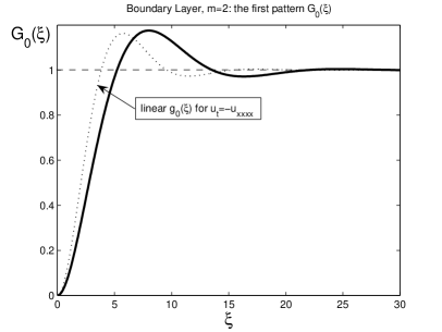
Figure 6. The unique stationary solution $G_{0}(\xi)$ of the problem (8.32).

Inner Region. This is also similar but there is a single nonlinear aspect that we have to address to. Thus, the only principal difference between (8.29) and (4.12) is that ${\bf B}^{*}(v)$ is a nonlinear operator, so we cannot immediately use the eigenfunctions expansion (7.17).

To this end, we recall that the BL-behaviour (8.33) actually implies that, in this critical case, we look for the so-called “mesa-like” asymptotics of solutions, which are supposed to be almost flat and to be independent of $y$ for $\tau\gg 1$ on compact subsets bounded away from the BL at $|y|\sim\varphi(\tau)$ (where (8.33) takes place). Such mesa-like asymptotics correspond to truly critical cases and are well-known in reaction-diffusion theory; see examples in [33, p. 59, 184]. According to this, it is correct to use the following approximation in the nonlinear term in ${\bf B}^{*}(v)$:

(8.34) $$v^{3}=\rho^{2}(\tau)v(1+o(1))\quad\mbox{for}\quad\tau\gg 1$$

on compact subsets bounded away from thin domains, where the “non-flat” BL-expansion (8.33) is in charge. Then

$$-(v^{3})_{yyyy}\mapsto-\rho^{2}(\tau)v_{yyyy}+...\,,$$

so that, to get back to the linear operator ${\bf B}^{*}$ in the equation, one needs to rescale the spatial variable as follows:

(8.35) $$\textstyle{v(y,\tau)=w(\eta,\tau),\quad\mbox{where}\quad\eta=\frac{y}{\sqrt{\rho(\tau)}}<\hat{\varphi}(\tau)=\frac{\varphi(\tau)}{\sqrt{\rho(\tau)}}\to+\infty.}$$

Then $w(\eta,\tau)$ solves the equation that in leading terms coincides with (7.16),

(8.36) $$\textstyle{w_{\tau}={\bf B}^{*}w+\frac{\rho^{\prime}}{\rho}\,\frac{1}{2}\,\eta w_{\eta}+...\,,}$$

where $+...$ denotes higher-order terms due to the sharp approximation (8.34). In comparison with the linear case (7.16), we observe the additional second term of the order $O\big{(}\frac{\rho^{\prime}}{\rho}\big{)}$ for $\tau\gg 1$, which is clearly negligible in view of (4.7)–(4.10). Moreover, $w_{\eta}\equiv 0$ on the subspace spanned by $\psi_{0}^{*}=1$, for which (8.34) and (7.5) hold.

We next introduce $\hat{w}$ according to the cut-off as in (7.14) at $\eta=\hat{\varphi}(\tau)\to+\infty$ given in (8.35). Then performing it first for the quasilinear equation for $w$ and next using the linearization as in (8.36), we arrive at

(8.37) $$\begin{matrix}\hat{w}_{\tau}={\bf B}^{*}\hat{w}+\frac{\rho^{\prime}}{\rho}\,\frac{1}{2}\,\eta\hat{w}_{\eta}\qquad\vskip 3.0pt plus 1.0pt minus 1.0pt\vskip 3.0pt plus 1.0pt minus 1.0pt\vskip 3.0pt plus 1.0pt minus 1.0pt\\ +\frac{1}{\rho^{2}}\big{[}(w^{3})_{\eta\eta\eta}\big{|}_{\eta=\hat{\varphi}}\delta(\eta-\hat{\varphi})+(w^{3})_{\eta\eta}\big{|}_{\eta=\hat{\varphi}}\delta^{\prime}(\eta-\hat{\varphi})\big{]}+...\,.\end{matrix}$$

Using in the last terms the BL estimates following from (8.33) (similar to (7.24)), and, as usual, applying (7.23) for the class of generic solutions, the eigenfunction expansion (7.17) for (8.37) yields the following asymptotic ODE for the first Fourier coefficient ($a_{0}>0$):

(8.38) $$\textstyle{a_{0}^{\prime}(\tau)=\gamma_{2}\sqrt{a_{0}(\tau)}\,\varphi(\tau)\psi_{0}\big{(}\frac{\varphi(\tau)}{\sqrt{a_{0}}}\big{)}+\gamma_{1}a_{0}^{\frac{2}{3}}(\tau)\varphi^{\frac{2}{3}}(\tau)\psi_{0}^{\prime}\big{(}\frac{\varphi(\tau)}{\sqrt{a_{0}}}\big{)}+...\,.}$$

It follow that, unlike a simpler equation (7.25), due to the extra “nonlinear” scaling (8.35), the Fourier coefficient $a_{0}(\tau)$ in (8.38) is now entering the oscillatory rescaled kernel $\psi_{0}$ and its derivative $\psi_{0}^{\prime}$. Since $\varphi(\tau)\to+\infty$ and $a_{0}(\tau)\to 0$ for the regularity (see (7.26)), the first term in (8.38) is leading that yields on substitution the asymptotics (5.12), (5.13):

(8.39) $$\textstyle{a_{0}^{\prime}=\hat{\gamma}\,a_{0}^{\frac{2}{3}}\varphi^{\frac{2}{3}}{\mathrm{e}}^{-d_{0}(\varphi/\sqrt{a_{0}})^{4/3}}C_{3}\cos\big{[}b_{0}\big{(}\frac{\varphi}{\sqrt{a_{0}}}\big{)}^{\frac{4}{3}}+C_{4}\big{]}+...\,.}$$

The asymptotic analysis of this ODE is similar. For instance, the following rate of convergence is obtained for the unperturbed “Gaussian” parabola:

(8.40) $$\textstyle{\varphi(\tau)\equiv 1:\quad a_{0}(\tau)\sim 3^{\frac{3}{2}}\,2^{-\frac{11}{2}}(\ln\tau)^{-\frac{3}{2}}\to 0,}$$

which shows the obvious result that the fundamental kernel parabolic shape for the shrinking point of $Q_{0}$ is regular.

In general, taking into account the main exponential term in (8.39) only, i.e., fixing the simplest approximating model

(8.41) $$\framebox{$a_{0}^{\prime}=-{\mathrm{e}}^{-d_{0}(\varphi/\sqrt{a_{0}})^{4/3}}\quad(a_{0}(\tau)>0),$}$$

we see that the critical $R(t)$ corresponds to

(8.42) $$\textstyle{\tilde{R}_{*}(t)\sim C(-t)^{\frac{1}{4}}\big{[}\ln|\ln(-t)|\,\big{]}^{\frac{3}{4}}\quad\mbox{as}\quad t\to 0^{-},}$$

where $C>0$ is arbitrary. Of course, unlike the linear case in (7.33), the constant $C$ in (8.42) cannot play a role in view of the scaling invariance of the PDE (8.27),

(8.43) $$u=A\hat{u},\quad x=\sqrt{A}\,\hat{x}\quad(A>0),$$

which changes the constant $C$ without changing the regularity of the point. Similar to (3.18)–(3.20), the scaling (8.43) itself implies (8.42) by choosing $A(t)=a_{0}(\tau)$ from (8.40).

It is not difficult to perform a more detailed study of the original ODE (8.39), though a too thorough analysis seems excessive. As usual, for the regularity, an oscillatory cut-off is necessary. Thus, it turns out that for the quasilinear (8.27) and linear (4.1) fourth-order parabolic equations, the regularity conditions (including the concepts and the methods) of boundary regularity analysis can be obtained in similar lines.

An analogous study can be done for the non-divergent thin film equation (TFE–4)

$$u_{t}=-(u^{2}u_{xxx})_{x},$$

though its existence-uniqueness theory is less developed, so the results will be more formal. Of course, the same techniques apply to the TFE–(2,2), with other distributions of the inner and outer derivatives in the differential form

$$u_{t}=-(u^{2}u_{xx})_{xx},$$

and to other PDEs with more general nonlinearities. Extensions to various quasilinear counterparts of the $2m$th-order parabolic equations (1.4) are also possible on the basis of the non self-adjoint spectral theory in [17].

8.4. Fourth-order hyperbolic equation: regularity via Hermitian spectral theory for a pencil

We recall that operator pencil theory fully occurred already in the regularity study for elliptic PDEs [49], and was later developed and extended in many papers; see [50, 71, 52, 53, 27] for references. Boundary regularity for hyperbolic PDEs is definitely less developed; see last pages of Kondrat’ev–Oleinik’s survey [50] of 1983 for some references. Note that, for fixed standard characteristic paraboloids posed for (8.44), the regularity problem falls into the scope of the results of Kondrat’ev’s “parabolic” paper [48]. The case of “expanding paraboloids” as $t\to 0^{-}$, similar to the above cases for the bi-harmonic equations and others, was not treated before by the same reasons (the lack of proper spectral theory and matching via a boundary layer approach, which are very difficult to fully justify).

Here, according to the principle (1.8), we very briefly discuss a new types of operator pencils that is needed to tackle other regularity problems. The simplest such model satisfying (1.8) is the linear fourth-order hyperbolic (wave) equation

(8.44) $$u_{tt}=-u_{xxxx}\quad\mbox{in}\quad Q_{0},$$

also known as the 1D linear beam equation. We consider the same Dirichlet problem as in (4.1) with two bounded initial functions $u(x,-1)=u_{0}(x)$ and $u_{t}(x,-1)=u_{1}(x)$. Concerning the fundamental solution and necessary spectral properties, we follow [29].

Thus, the fundamental solution of (8.44) has the self-similar form

(8.45) $$b_{0}(x,t)=\sqrt{t}\,\,F(y),\quad y=\frac{x}{\sqrt{t}},\quad\mbox{where}\quad b_{0}(x,0)=0,\quad b_{0t}(x,0)=\delta(x)$$

in the sense of bounded measures. The rescaled kernel $F_{0}=F_{0}(|y|)$ is symmetric and solves the ODE

(8.46) $$\textstyle{{\bf B}F\equiv-F^{(4)}-\frac{1}{4}\,F^{\prime\prime}y^{2}-\frac{1}{4}\,F^{\prime}y+\frac{1}{4}\,F=0\quad\mbox{in}\quad\mathbb{R},\quad\int F=1.}$$

Integrating (8.46) once yields

(8.47) $$\textstyle{-F^{\prime\prime\prime}-\frac{1}{4}\,F^{\prime}y^{2}+\frac{1}{4}\,Fy=0\quad\Longrightarrow\quad F(y)=\frac{1}{2\pi}\,\int\limits_{0}^{\infty}\frac{\sin z\cos(\sqrt{z}y)}{z^{3/2}}\,{\mathrm{d}}z.}$$

A WKBJ-type asymptotic analysis of the ODE (8.47) yields the behaviour like (1.8):

(8.48) $$\textstyle{F(y)\sim C_{1}y^{-\frac{11}{13}}\cos\big{(}\frac{y^{2}}{4}+C_{2}\big{)}\quad\mbox{as}\quad y\to+\infty,\quad C_{1}\not=0.}$$

Similar to (4.11), the first scaling is

(8.49) $$\begin{matrix}u(x,t)=v(y,\tau),\quad y=\frac{x}{\sqrt{-t}},\quad\tau=-\ln(-t),\qquad\,\,\,\qquad\vskip 3.0pt plus 1.0pt minus 1.0pt\vskip 3.0pt plus 1.0pt minus 1.0pt\vskip 3.0pt plus 1.0pt minus 1.0pt\\ v_{\tau\tau}+v_{\tau}+v_{\tau y}y={\bf B}^{*}v\equiv-v_{yyyy}-\frac{1}{4}\,y^{2}v_{yy}-\frac{3}{4}\,yv_{y}.\qquad\end{matrix}$$

Not paying enough attention to the functional setting of the operators involved in weighted $L^{2}$-spaces [29], we concentrate on the polynomial eigenfunctions of a quadratic pencil to appear; see Markus [63] for necessary concepts and theory of linear operator pencils. Namely, to find eigenfunctions, we set

(8.50) $$w(y,\tau)={\mathrm{e}}^{\lambda_{k}\tau}\psi_{k}^{*}(y)\quad\Longrightarrow\quad{\bf C}^{*}(\lambda_{k})\psi_{k}^{*}\equiv{\bf B}^{*}\psi_{k}^{*}-(\lambda_{k}^{2}+\lambda_{k})\psi_{k}^{*}-\lambda_{k}(\psi^{*}_{k})^{\prime}\,y=0.$$

Looking for finite polynomial eigenfunctions (recall that one needs two sets of eigenfunctions $\Psi^{*}=\{\psi_{k}^{*}(y),\,\phi_{k}^{*}(y)\}$ as well as the adjoint ones $\Psi=\{\psi_{k}(y),\,\phi_{k}(y)\}$ [29]),

(8.51) $$\textstyle{\psi_{k}^{*}(y),\,\,\,\phi_{k}^{*}(y)=y^{k}+...\quad\mbox{are $k$th-order polynomials,}}$$

substituting into (8.50) and keeping the higher-degree terms $\sim y^{k}$ yields the following quadratic equation for eigenvalues:

(8.52) $$\lambda_{k}^{2}+(k+1)\lambda_{k}+\frac{k(k-1)}{4}+\frac{3k}{4}=0.$$

This gives two, shifted by -1, series of eigenvalues,

(8.53) $$\lambda_{k}^{+}=-\frac{k}{2}\quad\mbox{and}\quad\lambda_{k}^{-}=-\frac{k}{2}-1\quad\mbox{for}\quad k=0,1,2,...\,.$$

Let us specify a half of those generalized Hermite polynomials, which is a complete closed set. There is another one obtained in a similar manner, which is obviously necessary for the second-order in $t$ PDE (8.44).

Proposition 8.1.

The eigenfunctions of the pencil $(\ref{p10})$ with the spectrum $\sigma_{+}=\{\lambda_{k}^{+}\}$ in $(\ref{p11})$ are given by the normalized polynomials

(8.54) $$\psi_{k}^{*}(y)=\frac{1}{\sqrt{k!}}\,\big{[}y^{k}+\sum_{j=1}^{[\frac{k}{4}]}\frac{1}{3^{j}\,j!}\,(y^{k})^{(4j)}\big{]},\quad k=0,1,2,...\,.$$

Assuming as usual that $\varphi(\tau)$ is a slow growing function (so (4.7), (4.8), … hold), we introduce the variable $z$ in (7.1) and the resulting BL-variables as in (7.2), where

(8.55) $$\textstyle{\xi=\varphi^{2}(\tau)(1-z),\quad z=\frac{y}{\varphi(\tau)},\quad D_{y}=-\varphi(\tau)D_{\xi}.}$$

Assuming that the class of generic solutions admitting a BL-representation is under scrutiny and performing the cut-off as in (7.14), where $\hat{v}_{\tau\tau}=v_{\tau\tau}H$, by the expansion (7.20) (we currently take into account the first coefficient only, with $\langle 1,F\rangle=1$ by the orthonormality, over the first half (8.54) of all the polynomials, and this defines the class of solutions involved), so eventually, by the asymptotics (8.48) yields

(8.56) $$\textstyle{a_{0}^{\prime\prime}+a_{0}^{\prime}+...\sim\gamma_{1}C_{3}a_{0}\varphi^{\frac{28}{13}}\,\cos\big{(}\frac{\varphi^{2}}{4}+C_{4}\big{)}+...\quad\big{(}\frac{28}{13}=3-\frac{11}{13}\big{)},}$$

where we omit all smaller terms containing $\varphi^{\prime},\,\varphi^{\prime\prime}$, and others. For slow varying coefficients $a_{0}(\tau)$, the leading term is indeed $a_{0}^{\prime}$, so, in this critical case, the governing ODE is

(8.57) $$\textstyle{\frac{a_{0}^{\prime}}{a_{0}}\sim\hat{\gamma}\,C_{3}\varphi^{\frac{28}{13}}\,\cos\big{(}\frac{\varphi^{2}}{4}+C_{4}\big{)}+...\quad\Longrightarrow\quad\ln|a_{0}(\tau)|\sim\int\limits^{\tau}\varphi^{\frac{28}{13}}\,\cos\big{(}\frac{\varphi^{2}}{4}+C_{4}\big{)}\,{\mathrm{d}}\tau.}$$

Clearly, unlike (8.21), by setting $\varphi^{2}(\tau)=s$, we see from (4.7) that a converging integral for the irregularity is impossible. However, this does not mean a “total” regularity. Actually, this again implies that the regularity issue here is rather subtle and, as usual for oscillatory kernels, can be achieved by a proper oscillatory cut-off of suitable slow growing $\varphi(\tau)$. For general $\varphi(\tau)$, a more delicate analysis of the ODE (8.56) with all the terms included is necessary, which leads to some technical questions. A full justification of the general approach then becomes difficult and even questionable.

Acknowledgement. The author would like to thank M. Kelbert for a fruitful discussion of the regularity-probability PDE issues and interesting historical comments on Khinchin’s results in 1924 and 1936 [45]. The author also thanks V.G. Maz’ya for help concerning general concepts of boundary regularity theory and for pointing out Fe${\rm\check{i}}$gin’s earlier results [25], S.R. Svirshchevskii for getting early and rare V.P. Miha${\rm\check{i}}$lov’s papers (in Russian) in 1961–63, and finally to A. Kyprianou for a short but informative conversation on Petrovskii’s and Khinchin’s contributions to the LIL and other probability issues.

Appendix A. Comment: On using majorizing order-preserving operators

It is clear that the main difficulty in establishing optimal regularity/irregularity criteria for higher-order linear parabolic PDEs such as (4.1), (1.4) (or third-order dispersion ones in (8.5) and (8.25) to be studied later on) is the fact that these flows do not obey the Maximum Principle and do not exhibit order-preserving features. As is well-known, the latter ones have been key for the heat equation (3.1) and other nonlinear second-order diffusion-reaction-absorption-convection-… equations; see references in [1, 2, 36, 76].

Therefore, before going into eigenfunction expansion techniques for solving the regularity problem for (4.1), we cannot avoid a temptation to briefly discussing a rather formal opportunity to deal with the traditional techniques based on the Maximum Principle even for the higher-order parabolic flow. This is about the idea of majorizing order-preserving flows for higher-order parabolic equations [31], which we explain relative to the poly-harmonic flow (1.4). Namely, given the rescaled oscillatory kernel (5.5), we construct the corresponding majorizing kernel $\bar{F}(y)>0$ such that

(A.1) $$\textstyle{|F(y)|\leq D_{m}\bar{F}(y)\quad\mbox{in}\quad\mathbb{R}^{N},\quad\mbox{where}\quad\int\bar{F}=1,}$$

and $D_{m}>1$ is a constant called the order deficiency (or order defect) of this majorizing kernel. It is clear that the optimal order deficiency is ($D_{1}^{*}=1$ since $F>0$)

(A.2) $$\textstyle{D_{m}^{*}=\int|F|>1,\quad\mbox{corresponding to the non-smooth kernel}\quad\bar{F}(y)=\frac{1}{D_{m}^{*}}\,|F(y)|}$$

(sometimes, dealing with not $C^{\infty}$ kernels $\bar{F}(y)$ is not convenient, especially when determining its eigenfunctions by differentiation via (5.16), with $F\mapsto\bar{F}$, etc.).

We then introduce the corresponding majorizing order-preserving integral evolution equation in $\mathbb{R}^{N}\times\mathbb{R}_{+}$ (it does not have a PDE representation in general) defined by the formal convolution

(A.3) $$\textstyle{\bar{u}(t)=\bar{b}(t)*\bar{u}_{0},\,\,\mbox{with}\,\,\bar{u}_{0}(x)\geq 0,\quad\mbox{where}\quad\bar{b}(x,t)=t^{-\frac{1}{2m}}\bar{F}(y),\quad y=\frac{x}{t^{1/2m}}.}$$

The corresponding comparison theorem is as follows [31]:

(A.4) $$\textstyle{|u_{0}(x)|\leq\frac{1}{D_{m}}\,\bar{u}_{0}(x)\quad\mbox{in}\quad\mathbb{R}^{N}\quad\Longrightarrow\quad|u(x,t)|\leq\bar{u}(x,t)\quad\mbox{in}\quad\mathbb{R}^{N}\times\mathbb{R}_{+}.}$$

The proof is straightforward in view of (A.1) via comparison of the solution of (A.3) with the parabolic flow

(A.5) $$\textstyle{u(x,t)=b(x-\cdot,t)*u_{0}(\cdot)\equiv t^{-\frac{1}{2m}}\,\int F\big{(}\frac{x-y}{t^{1/2m}}\big{)}\,u_{0}(y)\,{\mathrm{d}}y\quad\mbox{in}\quad\mathbb{R}^{N}\times\mathbb{R}_{+}.}$$

Indeed, subtracting (A.3) and (A.5) yields for the difference the desired inequality:

(A.6) $$\begin{matrix}w(x,t)=\bar{u}(x,t)-u(x,t)=t^{-\frac{1}{2m}}\int\big{[}\bar{F}(\cdot)\,\bar{u}_{0}-F(\cdot)\,u_{0}\big{]}\vskip 3.0pt plus 1.0pt minus 1.0pt\vskip 3.0pt plus 1.0pt minus 1.0pt\vskip 3.0pt plus 1.0pt minus 1.0pt\\ \geq t^{-\frac{1}{2m}}\int\big{[}\bar{F}(\cdot)\,\bar{u}_{0}-\frac{1}{D_{m}}\,|F(\cdot)|\,\bar{u}_{0}\big{]}=t^{-\frac{1}{2m}}\int\big{[}\frac{D_{m}\bar{F}(\cdot)-|F(\cdot)|}{D_{m}}\,\bar{u}_{0}\big{]}\geq 0,\end{matrix}$$

by the definition of the majorizing kernel (A.1). Since $\bar{F}>0$, i.e., the integral majorizing evolution (A.3) is order-preserving, solutions $\bar{u}(x,t)$ admit constructing super-solutions $\bar{U}(x,t)$ in the standard sense, i.e., the following comparison holds:

(A.7) $$\bar{U}(t)\geq\bar{b}(t)*\bar{u}_{0}\quad\Longrightarrow\quad 0<\bar{u}(x,t)\leq\bar{U}(x,t)\quad\mbox{in}\quad\mathbb{R}^{N}\times\mathbb{R}_{+}.$$

In [31], such comparison ideas resolved some asymptotic problems for semilinear parabolic equations related to Fujita critical exponents and around.

It is clear that to construct a majorizing comparison theory for the IBVPs in domains such as $Q_{0}$, further estimates of “Green’s function” corresponding to the “majorizing non-translational flow” (A.3) in $Q_{0}$ (as usual, such an estimate is expected to be related to (A.1)) are necessary. These are difficult questions, which are not discussed here. We just mention that such a true possibility would allow, in a reasonable simpler (and rigorous!) way, to get a proper upper estimates on solutions in $Q_{0}$ to prove that $u(0,0)=0$, which would guarantee its regularity, by constructing proper super-solutions. As a formal clue, it would be very efficiently and attractively easy to use Petrovskii’s ansatz (3.5),

(A.8) $$\textstyle{\bar{U}(x,t)\sim-\frac{1}{|\ln(-t)|^{1+\varepsilon_{1}}}\,{\mathrm{e}}^{{-d_{0}|x|^{\frac{2m}{2m-1}}}/{(-t)^{\frac{1}{2m-1}}}}+\frac{1}{\ln|\ln(-t)|},}$$

where we have replaced the Gaussian structure in (3.5) by that in the estimate (5.7), which is supposed to be true for the majorizing positive kernel $\bar{F}(y)$. As we will show (cf. (7.33) for $m=2$), the space-time structure (A.8) would give a correct critical behaviour for $R(t)$ as $t\to 0^{-}$, but we do not know if this can be justified in such a comparison way. (an open problem, but an extremely attractive one). We must admit that, besides some other fundamental open questions, in any case, unlike (3.5), using (A.8) for any $m\geq 2$ assumes complicated integral calculus to establish the validity of the integral inequality in (A.7). More importantly, such an integral majorizing approach cannot be used for any lower bound on $u(x,t)$ to get the irregularity counterpart, when $|u(0,0)|>0$. As one can see, corresponding alternative “minorizing” theory in similar lines cannot be constructed in principle. Therefore, we had no intention and in fact necessity to check whether functions such as (A.8) can satisfy (A.7) or similar integral inequalities. However, we state the following principal open problem: Is there any hope to get sharp regularity results by using majorizing-like calculus associated with some integral operator in $Q_{0}$ with a positive kernel?

References

- [1] U.G. Abdulla, Reaction-diffusion in irregular domains, J. Differ. Equat., 164 (2000), 321–354.
- [2] U.G. Abdulla, Multidimensional Kolmogorov-Petrovsky test for the boundary regularity and irregularity of solutions to the heat equation, Bound. Value Probl., 2 (2005), 181–199.
- [3] U.G. Abdulla, Wiener’s criterion at for the heat equation, Adv. Differ. Equat., 13 (2008), 457–488.
- [4] V.N. Aref’ev and L.A. Bagirov, Solutions of the heat equation in domains with singularities, Math. Notes, 64 (1998), 139–153.
- [5] W. Arendt and D. Daners, Varying domains: stability of the Dirichlet and the Poisson problem, Discrete Cont. Dyn. Syst., 21 (1008), 21–39 .
- [6] A.V. Arkhangelskii and V.M. Tikhomirov, Pavel Samuilovich Urysohn (1898–1924), Russian Math. Surveys, 55 (1998), 875–892.
- [7] T.Ya. Azizov and I.S. Iokhvidov, Linear Operators in Spaces with an Indefinite Metric, A Wiley-Intersci. Publ., Chichester/Singapore, 1989.
- [8] G. Barbatis, Explicit estimates on the fundamental solution of higher-order parabolic equations with measurable coefficients, J. Differ. Equat., 174 (2001), 442–463.
- [9] G. Barbatis, Sharp heat-kernel estimates for higher-order operators with singular coefficients, Proc. Edinb. Math. Soc. (2), 47 (2004), 53–67.
- [10] M.-F. Bidaut-Véron, V. Galaktionov, P. Grillot, and L. Véron, Singularities for a 2-dimensional semilinear elliptic equation with a non-Lipschitz nonlinearity, J. Differ. Equat., 154 (1999), 318–338.
- [11] M.S. Birman and M.Z. Solomjak, Spectral Theory of Self-Adjoint Operators in Hilbert Space, D. Reidel, Dordrecht/Tokyo, 1987.
- [12] M. Borsuk, Degenerate Elliptic Boundary-Value Problems of Second Order in Nonsmooth Domains, J. Math. Sci., 146 (2007), 6071–6212.
- [13] T. Carleman, Über das Neumann-Poincaresche Problem für ein Gebiet mit Ecken, Dissertation, Uppsala, 1916.
- [14] W. Chunpeng, W. Lihe, Y. Jingxue, and Z. Shulin, Hölder continuity of weak solutions of a class of linear equations with boundary degeneracy, J. Differ. Equat., 239 (2007), 99–131.
- [15] R. Courant and D. Hilbert, Methods of Mathematical Physics, Vol. II, R. Courant, Partial Differential Equations, Intersci. Publ., J. Wiley & Sons, New York/London, 1962.
- [16] R. Durrett, Probability: Theory and Examples, Wadworth Brooks/Cole Adv. Books Software, Pacific Grove, CA, 1991.
- [17] Yu.V. Egorov, V.A. Galaktionov, V.A. Kondratiev, and S.I. Pohozaev, Global solutions of higher-order semilinear parabolic equations in the supercritical range, Adv. Differ. Equat., 9 (2004), 1009–1038.
- [18] Yu.V. Egorov, V.A. Kondratiev, and B.-W. Schulze, On completeness of root functions of elliptic boundary problems in a domain with conical points on the boundary, Compt. Rendus Acad. Sci. Paris, Ser. I, 334 (2002), 649–654.
- [19] S.D. Eidelman, Parabolic Systems, North-Holland Publ. Comp., Amsterdam/London, 1969.
- [20] S.D. Eidelman, Parabolic equations, In: Modern Problems of Math. Fundam. Achiev., Vol. 63 (Part. Differ. Equat.), VINITI AN SSSR: 1990, Moscow, p. 244. English transl.: J. Soviet Math., 1991.
- [21] S. Eilstein, On weighted fractional integral inequalities, J. Funct. Anal., 185 (2001), 342–366.
- [22] U. Ellias, Eigenvalue problems for the equation , J. Differ. Equat., 29 (1978), 28–57.
- [23] L. Evans and R.F. Gariepy, Wiener’s critterion for the heat equation, Arch. Ration. Mech. Anal., 78 (1982), 293–314.
- [24] A.V. Faminskii, On the mixed problem for quasilinear equations of the third order, J. Math. Sci., 110 (2002), 2476–2507.
- [25] V.I. Fegin, Boundary value problems for quasi-elliptic equations in noncylindrical regions, Soviet Math. Dokl., 12 (1971), 634–638.
- [26] R.S. Fernandes and V.A. Galaktionov, Very singular similarity solutions and Hermitian spectral theory for semilinear odd-order PDEs, submitted.
- [27] J. Frehse and M. Kassmann, Nonlinear partial differential equations of fourth order under mixed boundary conditions, Math. Z., 254 (2006), 33–54.
- [28] V.A. Galaktionov, Sturmian nodal set analysis for higher-order parabolic equations and applications, Adv. Differ. Equat., 12 (2007), 669–720.
- [29] V.A. Galaktionov, Hermitian spectral theory and blow-up patterns for a fourth-order semilinear Boussinesq equation, Stud. Appl. Math., to appear.
- [30] V.A. Galaktionov, Blow-up in higher-order reaction-diffusion and wave equations: how factor occurs, Physica D, submitted.
- [31] V.A. Galaktionov and S.I. Pohozaev, Existence and blow-up for higher-order semilinear parabolic equations: majorizing order-preserving operators, Indiana Univ. Math. J., 51 (2002), 1321–1338.
- [32] V.A. Galaktionov and S.R. Svirshchevskii, Exact Solutions and Invariant Subspaces of Nonlinear Partial Differential Equations in Mechanics and Physics, ChapmanHall/CRC, Boca Raton, Florida, 2007.
- [33] V.A. Galaktionov and J.L. Vazquez, A Stability Technique for Evolution Partial Differential Equations. A Dynamical Systems Approach, Progr. in Nonl. Differ. Equat. and Their Appl., Vol. 56, Birkhäuser, Boston/Berlin, 2004.
- [34] M. Gevrey, Sue les équations aux dérivées partielles due type parabolique, J. math. pure appl. Paris (6), 9 (1913), 305–471; 10 (1914), 105–148.
- [35] A. Grigor’yan and M. Kelbert, On Hardy–Littlewood inequality for Brownian motion on Riemannian manifolds, J. London Math. Soc. (2), 62 (2000), 625–639.
- [36] M.A. Herrero, M. Ughi, and J.J.L. Velázquez, Approaching a vertex in a shrinking domain under a nonlinear flow, NoDEA, 11 (2004), 1–28.
- [37] Y. Ishikawa and M. Nakai, Regular and stable points in Dirichlet problem, Proc. Japan. Acad., Ser.A, 73 (1997), 1–4.
- [38] S.D. Ivasishen, Estimates of the Green function of the homogeneous first boundary value problem for a parabolic equation in a noncylindrical domain, Ukraninskii Mat. Zh., 21 (1969), 15–27.
- [39] T. Kato, Perturbation Theory for Linear Operators, Springer-Verlag, Berlin/New York, 1976.
- [40] M.V. Keldysh, Sur le problème de Dirichlet, Doklady Acad. Nauk SSSR (N.S.), 32 (1941), 308–309.
- [41] M.V. Keldysh, On the solvability and stability of the Dirichlet problem, Uspehi Matem. Nauk, 8 (1941), 171–231 (In Russian; MathRev. Reviever: J.D. Tamarkin); Amer. Math. Soc. Transl. (2), 51 (1966), 1–73.
- [42] M.V. Keldysh, On the characteristic values and characteristic functions of certain classes of non-self-adjoint equations, Doklady Akad. Nauk SSSR (N.S), 77 (1951), 11–14.
- [43] M.V. Keldysh, On certain cases of degeneration of equations of elliptic type on the boundary of a domain, Doklady Akad. Nauk SSSR (N.S), 77 (1951), 181–183.
- [44] O.D. Kellogg, Foundations of Potential Theory, Fred. Ungar Publ. Comp., New York, 1929.
- [45] A.Ya. Khinchin, Asymptotic Laws in Probability Theory, ONTI, Moscow, 1936. In [81, p. 57] and [82, p. 385] the following earlier Khinchin’s work (a book) is mentioned: A. Khintchine, Asymptotische Gesetze der Wahrscheinlichkeitsrechnung, Ergebnisse, 1933, and Petrvskii improved his result on the irregularity for the curve , .
- [46] A.N. Kolmogorov, I.G. Petrovskii, and N.S. Piskunov, Study of the diffusion equation with growth of the quantity of matter and its application to a biological problem, Byull. Moskov. Gos. Univ., Sect. A, 1 (1937), 1–26. English. transl. In: Dynamics of Curved Fronts, P. Pelcé, Ed., Acad. Press, Inc., New York, 1988, pp. 105–130.
- [47] V.A. Kondrat’ev, On the solvability of the first boundary value problem for elliptic equations, Soviet Math. Dokl., 2 (1961), 127–130.
- [48] V.A. Kondrat’ev, Boundary value problems for parabolic equations in closed regions, Trans. Moscow Math. Soc., Vol. 15, Amer. Math. Soc., Providence, RI, 1966, pp. 450–504.
- [49] V.A. Kondrat’ev, Boundary value problems for elliptic equations in domains with conical or angular points, Trans. Moscow Math. Soc., Vol. 16, Amer. Math. Soc., Providence, RI, 1967, pp. 227–313.
- [50] V.A. Kondrat’ev and O.A. Olenik, Boundary-value problems for partial differential equations in nonsmooth domains, Russian Math. Surveys, 38 (1983), 1–86.
- [51] V.A. Kozlov and V.G. Maz’ya, Asymptotic formula for solutions to elliptic equations near the Lipschitz boundary, Annali di Matem., 184 (2005), 185–213.
- [52] V.A. Kozlov, V.G. Maz’ya, and J. Rossmann, Elliptic Boundary Value Problems in Domains with Point Singularities, Math. Surveys Monogr., Vol. 52, Amer. Math. Soc., Providence, RI, 1997.
- [53] V.A. Kozlov, V.G. Maz’ya, and J. Rossmann, Spectral Problems with Corner Singularities of Solutions to Elliptic Equations, Math. Surveys Monogr., Vol. 85, Amer. Math. Soc., Providence, RI, 2001.
- [54] D.A. Labutin, Wiener regularity for large solutions of nonlinear equations, Ark. Mat., 41 (2003), 307–339.
- [55] E.M. Landis, Necessary and sufficient conditions for regularity of a boundary point in the Dirichlet problem for the heat conduction equation, Soviet Math. Dokl., 10 (1969), 380–384.
- [56] H. Lebesgue, Sur le problemè de Dirichlet, Rend. Circolo Mat. di Palermo, 24 (1907), 371–402.
- [57] H. Lebesgue, Sur le problemè de Dirichlet, Compt. Rendus Acad. Sci. Paris, 154 (1912), 335–337.
- [58] H. Lebesgue, Sur de cas d’impossibilité du problemè de Dirichlet, Comp. Rend. Soc. Math. France, 17 (1913), 48–50.
- [59] H. Lebesgue, Conditions de regularité, conditions d’irregularité, conditions d’impossibilité dans le problemè de Dirichlet, Compt. Rendus Acad. Sci. Paris, 178 (1924), 349–354.
- [60] J.L. Lions, Quelques méthodes de résolution des problèmes aux limites non linéaires, Dunod, Gauthier–Villars, Paris, 1969.
- [61] I.T. Mamedov, Boundary properties of solutions to second-order parabolic equations in domains with special symmetry, Math. Notes, 70 (2001), 347–362.
- [62] M. Marcus and L. Véron, Maximal solutions of the equation in arbitrary domains, Compt. Rend. Acad. Sci. Paris, Ser. I, 344 (2007), 299–304.
- [63] A.S. Markus, Introduction to the Spectral Theory of Polynomial Operator Pencils, Transl. Math. Mon., Vol. 71, Amer. Math. Soc., Providence, RI, 1988.
- [64] V.G. Maz’ya, On the continuity at a boundary point of solutions of quasi-linear elliptic equations, Vestnik Leningr. Univ., Math. Mech. Actronom., 25 (1970), 42–55; English transl.: Vestnik Leningr. Univ. Math., 3 (1976), 225–242.
- [65] V. Maz’ya, Behaviour of solutions to the Dirichlet problem for the biharmonic operator at a boundary point, Equadiff IV (Proc. Czechoslovak Conf. Differ. Equat. Appl., Prague, 1977), Lecture Notes Math., Vol. 703, Springer, Berlin, pp. 250–262.
- [66] V. Maz’ya, Unsolved problems connected with the Wiener criterion, The Legacy of Norbert Wiener: A Centennial Symposium (Cambridge, MA, 1994), Proc. Symp. Pure Math., Vol. 60, Amer. Math. Soc., RI, 1997, pp. 199–208.
- [67] V. Maz’ya, On the Wiener type regularity of a boundary point for the plyharmonic operator, Appl. Anal., 71 (1999), 149–165.
- [68] V. Maz’ya, The Wiener test for higher order elliptic equations, Duke Math. J., 115 (2002), 479–512.
- [69] V.G. Maz’ya, Private communication, September 2008.
- [70] V.G. Maz’ya and S.A. Nazarov, The apex of a cone can be irregular in Wiener’s sense for a fourth-order elliptic equation, Math. Notes, 39 (1986), 14–16.
- [71] V.G. Maz’ya and B.A. Plamenevskii, On the maximum principle for the biharmonic equation in a domain with conical points, Izv. Vyssh. Uchebn. Zaved. Mat., No. 2 (1981), 52–59.
- [72] V.P. Mihalov, The Dirichlet problem and the first mixed problem for a parabolic equation, Dokl. Akad. Nauk SSSR, 140 (1961), 303–306.
- [73] V.P. Mihalov, The Dirichlet problem for a parabolic equation. I, Mat. Sb. (N.S.), 61 (103) (1963), 40–64.
- [74] V.P. Mihalov, The Dirichlet problem for a parabolic equation. II, Mat. Sb. (N.S.), 62 (104) (1963), 140–159.
- [75] V.P. Mikhalov, Existence of the boundary value of a polyharmonic functions, Sib. Math. J., 46 (2005), 902–912.
- [76] J. Mossino and M. Ughi, On the regularity at shrinking points for the porous media equation, NoDEA, 7 (2000), 1–21.
- [77] M.A. Naimark, Linear Differential Operators, Part 1, Frederick Ungar Publ. Co., New York, 1967.
- [78] S.M. Nikol’skii, Boundary properties of functions defined on a region with angular points. I, II, III, Mat. Sb. N. S., 40(82) (1956), 303–318; 43(85) (1957), 127–144; 45(87) (1958), 181–194; English Transl.: Amer. Math. Soc. Transl., Series 2, Vol. 83, AMS, Providence, R.I., 1969.
- [79] O.A. Olenik and E.V. Radkevi, Second Order Differential Equations with Nonnegative Characteristic Form, Amer. Math. Soc., RI/Plenum Press, New York, 1973.
- [80] I.G. Petrovsky, Über das Irrfahrtproblem, Math. Ann., 109 (1934), 425–444.
- [81] J. Petrowsky, Über die Lösungen der ersten Randwertaufgabe der Wärmeleitungsgleichung, Uenye Zapiski Moscovsk. Gosud. Univ., No. 2 (1934), 55–59, Moscow, USSR (in German, with Russian summary).
- [82] I.G. Petrovsky, Zur ersten Randwertaufgabe der Wärmeleitungsleichung, Compositio Math., 1 (1935), 383–419.
- [83] I.G. Petrovskii, Lectures on Partial Differential Equations, Third Ed., Gos. Izdat. Fiz.-Mat. Lit., Moscow, 1961.
- [84] H. Poincaré, Sur le problème de la distribution électrique, Compt. Rendus Acad. Sci. Paris, 104 (1887), 44–46.
- [85] V. Rabinovich, B.-W. Schulze, and N. Tarhanov, Boundary value problems in oscillatory cuspidal wedges, Rocky Mount. J. Math., 34 (2004), 1399–1471.
- [86] A.A. Samarskii, V.A. Galaktionov, S.P. Kurdyumov, and A.P. Mikhailov, Blow-up in Quasilinear Parabolic Equations, Walter de Gruyter, Berlin/New York, 1995.
- [87] V.A. Solonnikov, On boundary value problems for linear parabolic systems of differential equations of the general form, Trudy Steklov Math. Inst., Vol. 83, Nauka, Moscow–Leningrad, 1965.
- [88] Ja.D. Tamarkin, Some General Problems of the Theory of Ordinary Differential Equations and Series Expansion of Arbitrary Functions, Tipografia M.P. Frolovoi, Petrograd, 1917 (in Russian).
- [89] P.S. Uryson, Zur ersten Randwertaufgabe der Potentialtheorie, Math. Zeitschrift, 23 (1925), 155–158.
- [90] M.A. Vainberg and V.A. Trenogin, Theory of Branching of Solutions of Non-Linear Equations, Noordhoff Int. Publ., Leiden, 1974.
- [91] L. Véron, Singularities of Solutions of Second Order Quasilinear Equations, Pitman Res. Notes Math. Ser., Vol. 353, Longman, Harlow, 1996.
- [92] L. Véron, Elliptic Equations Involving Measures, Stat. Part. Differ. Equat., Vol. I, pp. 593–712, Handbook Differ. Equat., North-Holland, Amsterdam, 2004.
- [93] N. Wiener, The Dirichlet problem, J. Math. and Phys. Mass. Inst. Tech., 3 (1924), 127–146; reprinted in: N. Wiener, Collected Works with Commentaries, Vol. I, ed. P. Masani, Mathematicians of Our Time 10, MIT Press, Cambridge, Mass., 1976, pp. 394–413.
- [94] I. Wood, Maximal -regularity for the Laplacian on Lipschitz domains, Math. Z., 255 (2007), 855–875.
- [95] S. Zaremba, Sur le principe de Dirichlet, Acta Math., 34 (1911), 293–316.