Graph-based Local Elimination Algorithms in Discrete Optimization

1 Introduction

The use of discrete optimization (DO) models and algorithms makes it possible to solve many practical problems in scheduling theory, network optimization, routing in communication networks, facility location, optimization in enterprise resource planning, and logistics (in particular, in supply chain management Dolg05 ). The field of artificial intelligence includes aspects like theorem proving, SAT in propositional logic (see Cook71 , GPFW97 ), robotics problems, inference calculation in Bayesian networks LaSpi88 , scheduling, and others.

Many real-life DO problems contain a huge number of variables and/or constraints that make the models intractable for currently available DO solvers. $NP$-hardness refers to the worst-case complexity of problems. Recognizing problem instances that are better (and easier for solving) than these ”worst cases” is a rewarding task given that better algorithms can be used for these easy cases.

Complexity theory has proved that universality and effectiveness are contradictory requirements to algorithm complexity. But the complexity of some class of problems decreases if the class may be divided into subsets and the special structure of these subsets can be used in the algorithm design.

To meet the challenge of solving large scale DO problems (DOPs) in reasonable time, there is an urgent need to develop new decomposition approaches BHT85 , RalG05 , Nowak . Large-scale DOPs are characterized not only by huge size but also by special or sparse structure. The block form of many DO problems is usually caused by the weak connectedness of subsystems of real systems. One of the first examples of large sparse linear programming (LP) problems which Dantzig started to study was a class of staircase LP problems for dynamic planning Dantzig49 , Dantzig73 , Dantzig81 . Further examples of staircase linear programs (see Fourer Fourer84 ) for multiperiod planning, scheduling, and assignment, and for multistage structural design, are included in a set of staircase test problems collected by Ho & Loute HoLo81 . Staircase linear programs have also been derived in connection with linearly constrained optimal control and stochastic programming Wets61 . Problems of optimal hotel apartments assignment, linear dynamic programming, labor resources allocation, control on hierarchic structures (usually having tree-like structure), multistage integer stochastic programming, network problems may be considered as examples of DO problems which have staircase structure (see Shch80 , Shch83 ). The well known SAT problem stems from classical investigations by logicians of propositional satisfiability and has over 90 years of history. It is possible to represent a SAT problem as a sparse DO problem Hook . Some applied facility location problems can be formulated as set covering problems, set packing problems, node packing problems Nem88 . Another class of sparse DO problems is a production lot-sizing problem Nem88 . The frequency assignment problem (FAP) Koster99 in mobile telephone systems communication is a hard problem as it is closely related to the graph coloring problem. One of the well known decomposition approaches to solving DOPs is Lagrangean decomposition that consists of isolating sets of constraints to obtain separate and easy to solve DO problems. Lagrangean decomposition removes the complicating constraints from the constraint set and inserts them into the objective function. Most Lagrangean decomposition methods deal with special row structures. Block angular structures with complicating variables and with complicating variables and constraints can be decomposed using Benders decomposition Bend62 and cross decomposition VanRoy . The Dantzig-Wolfe decomposition principle of LP has its equivalent in integer programming VandS00 . This approach uses the reformulation that gives rise to an integer master problem, whose typically large number of variables is dealt with implicitly by using an integer programming column generation procedure, also known as branch-and-price algorithm BJNSV98 that allows solving large-scale DOPs in recent years. Nemhauser (Nem94 , p. 9) mentioned, however, that

… the overall idea of using branch and bound with linear programming relaxation has not changed.

Usually, DOPs from applications have a special structure, and the matrices of constraints for large-scale problems have a lot of zero elements (sparse matrices). Among decomposition approaches appropriate for solving such problems we mention poorly known local decomposition algorithms using the special block matrix structure of constraints and half-forgotten nonserial dynamic programming algorithms (NSDP) (Bertele & Brioschi BerBri69a , BerBri69b , BerBri , Dechter Decht92 , Dechter , Dechter2001 , Dechter03 , Hooker Hook ) which can exploit sparsity in the dependency graph of a DOP and allow to compute a solution in stages such that each of them uses results from previous stages.

Recently, there has been growing interest in graph-based approaches to decomposition Bodl03 ; one of them is tree decomposition (TD). Courcelle Cour90 and Arnborg et al. Arn91 showed that several $NP$-hard problems posed in monadic second-order logic can be solved in polynomial time using dynamic programming techniques on input graphs with bounded treewidth. Thus graph-based decomposition approaches have gained importance. Graph-based structural decomposition techniques, e.g., nonserial dynamic programming (NSDP) (Bertele, Brioschi BerBri , Esogbue & Marks EsogMar74 , Hooker Hook , Martelli & Montanari MartMont72 , Mitten & Nemhauser Mitt63 , Neumaier & Shcherbina Neus , Rosenthal Rosen , Shcherbina Soa07k ), Wilde & Beightler Wilde67 and its modifications (bucket elimination Dechter , Seidel’s invasion method Sei81 ), tree decomposition combined with dynamic programming DechtPea , BodKos07 and its variants PanGo96 , hypertree Gottlob00 and hinge decomposition JGC94 , GJC94 are promising decomposition approaches that allow exploiting the structure of discrete problems in constraint satisfaction (CS) Fr92 and DO.

It is important that aforementioned methods use just the local information (i.e., information about elements of given element’s neighborhood) in a process of solving discrete problems. It is possible to propose a class of local elimination algorithms as a general framework that allows to calculate some global information about a solution of the entire problem using local computations JLO90 , LaSpi88 , SheSha86 . Note that a main feature in aforementioned problems is the locality of information, a definition of elements’ neighborhoods and studying them.

The use of local information (see Zhur98 , ZhurL95 , Fink65 , Soa08 , Urrut2007 ) is very important in studying complex discrete systems and in the development of decomposition methods for solving large sparse discrete problems; these problems simultaneously belong to the fields of discrete optimization Nem88 , Flo95 , PardDu , PardWolk , Serg03 , artificial intelligence Dechter , Gottlob08 , Nea , Pea4 , and databases Beeri83 . In linear algebra, multifrontal techniques for solving sparse systems of linear equations were developed (see Rose72 ); these methods are also of the decomposition nature. In Zhur98 , local algorithms for computing information are introduced. A local algorithm $A$ examines the elements in the order specified by an ordering algorithm $A_{\pi}$, calculates the function $\phi$ whose value at each step determines the form of the information marks, and labels the element using local information about the elements in its neighborhood. The function $\phi$ that induces the algorithm depends on two variables: the first ranges over the set of all elements and the second ranges over the set of neighborhoods. Local decomposition algorithms (see Shch80 , Shch83 ) in DO problems have a specific feature. Namely, rather than calculating predicates, they use Bellman’s optimality principle Bell to find optimal solutions of the subproblems corresponding to blocks of the DO problem. A step of the local algorithm $\mathfrak{A}$ changes the neighborhood and replaces the index $p$ by $p+1$ (however, one can increment the index by an arbitrary number replacing $S_{p}$ by $S_{p+\rho}$; at each step of the algorithm, for every fixed set of variables of the boundary ring, the values of the variables of the corresponding neighborhood are stored, which is an important difference of the local algorithm $\mathfrak{A}$ from $A$: information about variables in the solutions of the subproblems is stored rather than information about the predicates. Zhuravlev proposed to call it indicator information.

Tree and branch decomposition algorithms have been shown to be effective for DO problems like the traveling salesman problem CS03 , frequency assignment Koster99 etc. (see a survey paper Hicks ). A paper Arn85 surveys algorithms that use tree decompositions. Most of works based on tree decomposition approach only present theoretical results Jegou_comp , see the recent surveys Hicks , Soa07t . Thus these methods are not yet recognized tools of operations research practitioners.

Some implementations of NSDP are known BerBri , Fern88 , however, generally, it remains some ”obscure” tool for operations research modellers. Usually, tree decomposition approaches and NSDP are considered in the literature separately, without reference to the close relation between these methods. We try to indicate a close relation between these methods.

A need to solve large-scale discrete problems with special structure using graph-based structural decomposition methods provides the main motivation for this chapter. Here we try to answer a number of questions about tree decomposition and NSDP in solving DO problems. What are they? How and where can they be applied? What consists a connection between different structural decomposition methods, such as tree decomposition and nonserial dynamic programming?

The aim of this paper is to provide a review of structural decomposition methods and to give a unified framework in the form of local elimination algorithms Soa08 . We propose here the general approach which consists of viewing a decomposition of some DO problem as being represented by a DAG whose nodes represent subproblems that only contain local information. The nodes are connected by arcs that represent the dependency of the local information in the subproblems. A subproblem that is higher in the hierarchy may use the information (or knowledge) obtained in the dependent subproblems.

This paper is organized as follows: In section 2 we introduce local elimination algorithms for solving discrete problems. In Section 3 we survey necessary terminology and notions for discrete optimization problems and their graph representations. In Section 4 we consider local variable elimination schemes for solving DO problems with constraints and discuss a classification of dynamic programming (DP) computational procedure. Elimination Game is introduced. Application of the bucket elimination algorithm from CS to solving DO problems is done. Then, in Section 5, we consider a local block elimination scheme and related notions. As a promising abstraction approach of solving DOPs we define clustering that merges several variables into a single meta-variable. This allows us to create a quotient (condensed) graph and apply a local block elimination algorithm. In Section 6 a tree decomposition scheme is introduced. Connection of of the local elimination algorithmic schemes with tree decomposition and a way of transforming the DAG of computational local elimination procedure to tree decomposition are discussed.

2 Local elimination algorithms for solving discrete problems

The structure of discrete optimization problems is determined either by the original elements (e.g., variables) with a system of neighborhoods specified for them and with the order of searching through those elements using a local elimination algorithm or by various derived structures (e.g., block or tree-block structures). Both original and derived structures can be specified by the so called structural graph. The structural graph can be the interaction graph of the original elements (for example, between the variables of the problem) or the quotient george (condensed Harary ) graph. The quotient graph can be obtained by merging a set of original elements (for example, a subgraph) into a condensed element. The original subset (subgraph) that formed the condensed element is called the detailed graph of this element.
A local elimination algorithm (LEA) Soa08 eliminates local elements of the problem’s structure defined by the structural graph by computing and storing local information about these elements in the form of new dependencies added to the problem. Thus, the local elimination procedure consists of two parts:

• The forward part eliminates elements, computes and stores local solutions, and finally computes the value of the objective function;

• The backward part finds the global solution of the whole problem using the tables of local solutions; the global solution gives the optimal value of the objective function found while performing the forward part of the procedure.

The LEA analyzes a neighborhood $Nb(x)$ of the current element $x$ in the structural graph of the problem, applies an elimination operator (which depends on the particular problem) to that element, calculates the function $h(Nb(x))$ that contains local information about $x$, and finds the local solution $x^{*}(Nb(x))$. Next, the element $x$ is eliminated, and a clique is created from the elements of $Nb(x)$. The elimination of elements and the creation of cliques changes the structural graph and the neighborhoods of elements. The backward part of the local elimination algorithm reconstructs the solution of the whole problem based on the local solutions $x^{*}(Nb(x))$.

The algorithmic scheme of the LEA is a DAG in which the vertices correspond to the local subproblems and the edges reflect the informational dependence of the subproblems on each other.

3 Discrete optimization problems and their graph representations

3.1 Notions and definitions

Consider a sparse DOP in the following form

$$F(x_{1},x_{2},\ldots,x_{n})=\sum_{k\in K}f_{k}(X^{k})\rightarrow\max$$ (1)

subject to the constraints

$$g_{i}(X_{S_{i}})~{}R_{i}~{}0,~{}~{}i\in M=\{1,2,\ldots,m\},$$ (2)

$$x_{j}\in D_{j},~{}~{}j\in N=\{1,\ldots,n\},$$ (3)

where
$X=\left\{x_{1},\dots,x_{n}\right\}$ is a set of discrete variables, $X^{k}\subseteq\{x_{1},x_{2},\ldots,x_{n}\},k\in K=\left\{1,2,\ldots,t\right\},$ $t$ – number of components in the objective function, $S_{i}\subseteq\{1,2,\ldots,n\},~{}R_{i}\in\{\leq,=,\geq\},i\in M$; $D_{j}$ is a finite set of admissible values of variable $x_{j},~{}~{}j\in N$. Functions $f_{k}(X^{k}),~{}~{}k\in K$ are called components of the objective function and can be defined in tabular form. We use here the notation: if $S=\{j_{1},\ldots,j_{q}\}$ then $X_{S}=\{x_{j_{1}},\ldots,x_{j_{q}}\}$.
In order to avoid complex notation, without loss of generality, we consider further a DOP with linear constraints and binary variables:

$$\max_{X}f(X)=\max_{X}\sum_{k\in K}f_{k}(X^{k}),$$ (4)

subject to

$$A_{iS_{i}}X_{S_{i}}\leq b_{i},~{}i\in M=\{1,2,\ldots,m\},$$ (5)

$$x_{j}=0,1,~{}j\in N=\{1,\ldots,n\}.$$ (6)

We shall consider further a linear objective function (7):

$$f(x_{1},\ldots,x_{n})=f(X)=C_{N}X_{N}=\sum_{j=1}^{n}c_{j}x_{j}\rightarrow\max$$ (7)

Definition 1

BerBri . Variables $x\in X$ and $y\in X$ interact in DOP with constraints (we denote $x\sim y$) if they both appear either in the same component of the objective function, or in the same constraint (in other words, if variables are both either in a set $X^{k}$, or in a set $X_{S_{i}}$).

Introduce a graph representation of the DOP. Description of the DOP structure may be done with various detailization. The structural graph of the DOP defines which variables are in which constraints. Structure of a DOP can be defined either by interaction graph of initial elements (variables in the DOP) or by various derived structures, e.g., block structures, block-tree structures defined by so called quotient (condensed or compressed Ash95 , AshLiu98 , HendRoth98 ) graph.

Concrete choice of a structural graph of the DOP defines different local elimination schemes: nonserial dynamic programming, block decomposition, tree decomposition etc.

If the DOP is divided into blocks corresponding to subsets of variables (meta-variables) or to subsets of constraints (meta-constraints), then block structure can be described by a structural quotient (condensed) graph, whose meta-nodes correspond to subsets of the variables of blocks and meta-edges correspond to adjacent blocks (see below, in section 5.1).

An interaction graph BerBri (dependency graph by HOOKER Hook ) represents a structure of the DOP in a natural way.

Definition 2

BerBri . Interaction graph of the DOP is an undirected graph $G=(X,E)$, such that

• Vertices $X$ of $G$ correspond to variables of the DOP;

• Two vertices of $G$ are adjacent iff corresponding variables interact.

Further, we shall use the notion of vertices that correspond one-to-one to variables.

Definition 3

Set of variables interacting with a variable $x\in X$ is denoted by $Nb(x)$ and called the neighborhood of the variable $x$. For corresponding vertices a neighborhood of a vertex $x$ is a set of vertices of interaction graph that are linked by edges with $x$. Denote the latter neighborhood as $Nb_{G}(x)$.

Introduce the following notions:

1. Neighborhood of a set $S\subseteq X$, $Nb_{G}(S)=\bigcup_{x\in S}Nb_{G}(x)-S$.

2. Closed neighborhood of a set $S\subseteq X$, $Nb_{G}[S]=Nb_{G}(S)\cup S$.

4 Local variable elimination algorithms in discrete optimization

4.1 Nonserial dynamic programming and
classification of DP formulations

NSDP exploits only local computations to solve global discrete optimization problems and is, therefore, a particular instance of local elimination algorithm. It appeared in 1961 with Aris Aris61 (see BeiJohn65 , BerBri69a , BerBri69b , Mitt63 ) but is poorly known to the optimization community. This approach is used in Artificial Intelligence under the names ”Variable Elimination” or ”Bucket Elimination” Dechter . NSDP being a natural and general decomposition approach to sparse problems solving, considers a set of constraints and an objective function as recursively computable function Hook . This allows to compute a solution in stages such that each of them uses results from previous stages. This requires a reduced effort to find the solution.
Thus, the DP algorithm can be applied to find the optimum of the entire problem by using the connected optimizations of the smaller DO subproblems with the aid of existing optimization solvers.

It is worth noting that NSDP is implicit in Hammer and Rudeanu’s ”basic method” for pseudoboolean optimization HamRud68 . Crama, Hansen, and Jaumard Crama90 discovered that the basic method can exploit the structure of a DOP with the usage of so-called co-occurrence graph (interaction graph). It was found that the complexity of the algorithm depends on induced width of this graph, which is defined for a given ordering of the variables. Consideration of the variables in the right order may result in a smaller induced width and faster solution Hook02 .
In BerBri mostly DO problems without constraints were considered. Here, we consider an application of NSDP variable elimination algorithm to solving DO problems with constraints.

One of the most useful graph-based interpretations is a representation of computational DP procedure as a direct acyclic graph (DAG) soa07din whose vertices are associated with subproblems and whose edges express information interdependence between subproblems.

Every DP algorithm has an underlying DAG structure that usually is implicit das : the dependencies between subproblems in a DP formulation can be represented by a DAG. Each node in the DAG represents a subproblem. A directed edge from node $A$ to node $B$ indicates that the solution to the subproblem represented by node $A$ is used to compute the solution to the subproblem represented by node $B$ (Fig.1). The DAG is explicit only when we have a graph optimization problem (say, a shortest path problem). Having nodes $u_{1},\ldots,u_{k}$ point to $v$ means ”subproblem $v$ can only be solved once the solutions to $u_{1},\ldots,u_{k}$ are known” (Fig. 2).

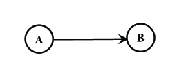
Figure 1: Precedence of subproblems A and B.

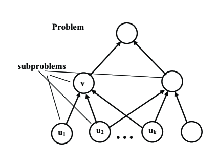
Figure 2: Underlying DAG of subproblems.

Thus, the DP formulation can be described by the DAG of the computational procedure of a DP algorithm (underlying DAG das ). Li & Wah Wah88 proposed to classify various DP computational procedures or DP formulations on the basis of the dependencies between subproblems from the underlying DAG.

The nodes of the DAG can be organized into levels such that subproblems at a particular level depend only on subproblems at previous levels. In this case, the DP procedure (formulation) can be categorized as follows. If subproblems at all levels depend only on the results of subproblems at the immediately preceding levels, the procedure (formulation) is called a serial DP procedure (formulation), otherwise, it is called a nonserial DP procedure (formulation).

Example 1

The simplest optimization problem is the serial unconstrained discrete optimization problem BerBri

$$\max_{X}f(X)=\max_{X}\sum_{i\in K}f_{i}(X^{i}),$$

where $X=\left\{x_{1},\dots,x_{n}\right\}$ is a set of discrete variables.

$$K=\left\{1,2,\ldots,n-1\right\};~{}~{}X^{i}=\left\{x_{i},x_{i+1}\right\}.$$

In fig. 3 it is shown an interaction graph of the serial DO problem.

Figure 3: Interaction graph for the serial formulation of unconstrained DOP.

4.2 Discrete optimization problem with constraints

Consider the DOP (7), (5), (6) and suppose without loss of generality that variables are eliminated in the order $x_{1},\ldots,x_{n}$. Using the local variable elimination scheme eliminate the first variable $x_{1}$. $x_{1}$ is in a set of constraints with the indices in $U_{1}$:

$$U_{1}=\{i\mid x_{1}\in S_{i}\}$$

Together with $x_{1}$, constraints in $U_{1}$ contain variables from $Nb(x_{1})$.

The following subproblem $P_{1}$ corresponds to the variable $x_{1}$ of the DOP:

$$h_{x_{1}}(Nb(x_{1}))=\max_{x_{1}}\{c_{1}x_{1}|A_{iS_{i}}X_{S_{i}}\leq b_{i},~{}i\in U_{1},~{}x_{j}=0,1,~{}x_{j}\in Nb[x_{1}]\}$$

Then the initial DOP can be transformed in the following way:

$$\max_{x_{1},\ldots,x_{n}}\Bigl{\{}\sum C_{N}X_{N}|A_{iS_{i}}X_{S_{i}}\leq b_{i},~{}~{}i\in M,~{}x_{j}=0,1,~{}j\in N\Bigr{\}}=$$

$$\max_{x_{2},\ldots,x_{n}}\{C_{N-\{1\}}X_{N-\{1\}}+h_{x_{1}}(Nb(x_{1})|A_{iS_{i}}X_{S_{i}}\leq b_{i},~{}i\in M-U_{1},~{}x_{j}=0,1,~{}j=2,\ldots,n\}$$

The last problem has $n-1$ variables; from the initial DOP were excluded constraints with the indices in $U_{1}$ and from the objective function the term $c_{1}x_{1}$; there appeared a new objective function term $h_{x_{1}}(Nb(x_{1}))$. Due to this fact the interaction graph associated with the new problem is changed: a vertex $x_{1}$ is eliminated and its neighbors have become connected (due to the appearance a new term $h_{x_{1}}(Nb(x_{1}))$ in the objective). It can be noted that a graph induced by vertices of $Nb(x_{1})$ is complete, i.e. is a clique. Denote the new interaction graph $G^{1}$ and find all neighborhoods of variables in $G^{1}$. NSDP eliminates the remaining variables one by one in an analogous manner. We have to store tables with optimal solutions at each stage of this process.
At the stage $n$ of the described process we eliminate a variable $x_{n}$ and find an optimal value of the objective function. Then a backward step of the local elimination procedure is performed using the tables with solutions.

4.3 Elimination game, combinatorial elimination process, and underlying DAG of the LAE computational procedure

Consider a sparse discrete optimization problem (1) — (3) whose structure is described by an undirected interaction graph $G=(X,E)$. Solve this problem with a local elimination algorithm (LEA). LEA uses an ordering $\alpha$ of $X$ RoTaLu76 : Given a graph $G=(X,E)$ an ordering $\alpha$ of $X$ is a bijection $\alpha:X\leftrightarrow\{1,2,\ldots,n\}$ where $n=|X|$.
$G_{\alpha}$ and $X_{\alpha}$ are correspondingly an ordered graph and an ordered vertex set. Sometimes the ordering will be denoted as $x_{1},\ldots,x_{n}$, i.e. $\alpha(x_{i})=i$ and $i$ will be considered as an index of the vertex $x_{i}$.

In $G_{\alpha}$, a monotone neighborhood $\overline{Nb}^{\alpha}_{G}(x_{i})$ (Blair93 , RoTaLu76 ) of $x_{i}\in X$ is a set of vertices monotonely adjacent to a vertex $x_{i}$, i.e.

$$\overline{Nb}^{\alpha}_{G}(x_{i})=\{x_{j}\in Nb_{G}(x_{i})|j>i\}.$$

The graph $G_{x}$ Rose72 obtained from $G=(X,E)$ by

• adding edges so that all vertices in $Nb_{G}(x)$ are pairwise adjacent, and

• deleting $x$ and its incident edges

is the $x$–elimination graph of $G$. This process is called the elimination of the vertex $x$.

Given an ordering $x_{1},x_{2},\ldots,x_{n}$, the LEA proceeds in the following way: it subsequently eliminates $x_{1},x_{2},\ldots,x_{n}$ in the current graph and computes an associated local information about vertices from $h_{x_{i}}(Nb(x_{i}))$ Soa08 . This can be described by the combinatorial elimination process Rose72 :

$$G_{0}=G,G_{1},\ldots,G_{j-1},G_{j},\ldots,G_{n}$$

where $G_{j}$ is the $x_{j}$–elimination graph of $G_{j-1}$ and $G_{n}=\emptyset$.

The process of interaction graph transformation corresponding to the LEA scheme is known as Elimination Game which was first introduced by Parter Part as a graph analogy of Gaussian elimination. The input of the elimination game is a graph $G$ and an ordering $\alpha$ of $G$ (i.e. $\alpha(x)=i$ if $x$ is $i$-th vertex in the ordering $\alpha$). Elimination Game according to HEKP01 consists in the following. At each step $i$, the neighborhood of vertex $x_{i}$ is turned into a clique, and $x_{i}$ is deleted from the graph. This is referred to as eliminating vertex $x_{i}$. We obtain a graph $G_{x_{i}}^{(i)}$. The filled graph $G^{+}_{\alpha}=(X,~{}E^{+}_{\alpha})$ is obtained by adding to $G$ all the edges added by the algorithm. The resulting filled graph $G_{\alpha}^{+}$ is a triangulation of $G$ (FULKERSON & GROSS FulkGross ), i.e., a chordal graph.

Let us introduce the notion for the elimination tree (etree) Liu90 . Given a graph $G=(X,E)$ and an ordering $\alpha$, the elimination tree is a directed tree $\overrightarrow{T}_{\alpha}$ that has the same vertices $X$ as $G$ and its edges are determined by a parent relation defined as follows: the parent $x$ is the first vertex (according to the ordering $\alpha$) of the monotone neighborhood $\overline{Nb}^{\alpha}_{G^{+}_{\alpha}}(x)$ of $x$ in the filled graph $G^{+}_{\alpha}$.
Using the parent relation introduced above we can define a directed filled graph $\overrightarrow{G}^{+}_{\alpha}$.
The underlying DAG of a local variable elimination scheme can be constructed using Elimination Game. At step $i$, we represent the computation of the function $h_{x_{i}}(Nb_{G_{x_{i-1}}}(x_{i}))$ as a node of the DAG (corresponding to the vertex $x_{i}$). Then, this node containing variables $(x_{i},Nb_{G_{x_{i-1}}}^{(i-1)}(x_{i}))$ is linked with a first $x_{j}$ (accordingly to the ordering $\alpha$) which is in $Nb_{G_{x_{i-1}}^{(i-1)}}(x_{i})$.
It is easy to see that the elimination tree is the DAG of the computational procedure of the LEA.

Example 2

Consider a DOP (P) with binary variables:

$$2x_{1}+3x_{2}+~{}x_{3}+5x_{4}+4x_{5}+6x_{6}+~{}x_{7} \rightarrow\max$$

$$3x_{1}+4x_{2}+~{}x_{3}~{}~{}~{}~{}~{}~{}~{}~{}~{}~{}~{}~{}~{}~{}~{}~{}~{}~{}~{}~{}~{}~{}~{}~{}~{}~{} \leq 6,~{}~{}(C_{1})$$

$$~{}~{}~{}~{}~{}~{}~{}~{}2x_{2}+3x_{3}+3x_{4}~{}~{}~{}~{}~{}~{}~{}~{}~{}~{}~{}~{}~{}~{}~{}~{}~{}~{} \leq 5,~{}~{}(C_{2})$$

$$~{}~{}~{}~{}~{}~{}~{}~{}2x_{2}~{}~{}~{}~{}~{}~{}~{}~{}~{}~{}~{}~{}~{}~{}~{}~{}+3x_{5}~{}~{}~{}~{}~{}~{}~{} \leq 4,~{}~{}(C_{3})$$

$$~{}~{}~{}~{}~{}~{}~{}~{}~{}~{}~{}~{}~{}~{}~{}~{}2x_{3}~{}~{}~{}~{}~{}~{}~{}~{}~{}~{}~{}~{}~{}~{}~{}~{}+3x_{6}+2x_{7}~{} \leq 5,~{}~{}(C_{4})$$

$$~{}x_{j}=0,1,~{}j=1,\ldots,7.~{}~{}~{}~{}~{}~{}~{}~{}~{}~{}~{}~{}~{}~{}~{}~{}~{}~{}~{}~{}~{}~{}~{}~{}~{}~{}~{}~{}~{}~{}~{}~{}~{}$$

The interaction graph is shown in Fig. 4 (a). Elimination Game results and graphs $G_{x_{i}}^{(i)}$ are in Fig. 5. Associated underlying DAG of NSDP procedure for the variable ordering $\{x_{5},x_{2},x_{1},x_{4},x_{3},x_{6},x_{7}\}$ is shown in Fig. 4 (b).

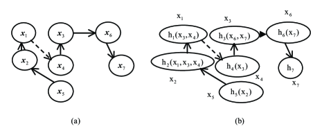
Figure 4: Elimination tree of the DOP (a) Computing the information while eliminating variables in the LEA computational procedure (b) (example 2).

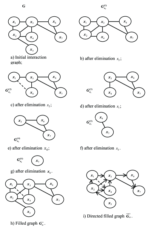
Figure 5: Elimination Game. Fill-in is represented by dashed lines

4.4 Bucket elimination

Bucket elimination (BE) is proposed in Dechter as a version of NSDP for solving CSPs. Now, we consider a modification of the BE algorithm for solving DOPs. The BE algorithm works as follows: Assume we are given an order $x_{1},\ldots,x_{n}$ of the variables of the DOP. BE starts by creating $n$ ”buckets”, one for each variable $x_{j}$. BE algorithm uses as input ordered set of variables and a set of constraints. To each variable $x_{j}$ is corresponded a bucket $\Sigma^{(x_{j})}$, i.e., a set of constraints and components of objective function built as follows: In the bucket $\Sigma^{(x_{j})}$ of variable $x_{j}$ we put all constraints that contain $x_{j}$ but do not contain any variable having a higher index. We now iterate on $j$ from $n$ to 1, eliminating one bucket at a time. Algorithm finds new components of the objective applying so called ”elimination operator” (in our case the latter consists on solving associated DO subproblems) to all constraints and components of the objective function of the bucket under consideration. New components of the objective function reflecting an impact of variable $x_{j}$ on the rest part of the DO problem, are located in corresponding lower buckets.
Consider an application of BE to solving the DOP with constraints from Example 2. We use an elimination ordering $\alpha:~{}\{x_{5},x_{2},(x_{1},x_{4}),x_{3},(x_{6},x_{7})\}$. Variables $(x_{1},x_{4})$ shall be eliminated in block since they are indistinguishable. Build buckets (subsets of constraints) beginning from last (due order $\alpha$) block $(x_{6},x_{7})$. A bucket $\Sigma^{(x_{6},x_{7})}$ includes all constraints of the DOP containing the variables $x_{6},~{}x_{7}$, i.e., the bucket $\Sigma^{(x_{6},x_{7})}$ consists of constraint $C_{4}$: $\Sigma^{(x_{6},x_{7})}=\{C_{4}\}.$ Similarly: $\Sigma^{(x_{3})}=\{C_{1},C_{2}\},~{}~{}\Sigma^{(x_{1},x_{4})}=\emptyset,~{}~{}\Sigma^{(x_{2})}=\{C_{3}\},~{}~{}\Sigma^{(x_{5})}=\emptyset$.
We solve a DO subproblem associated with the bucket $\Sigma^{(x_{6},x_{7})}$:
For each binary assignment $x_{3}$, we compute values $x_{6},x_{7}$ such that

$$h_{x_{6},x_{7}}(x_{3})=\max_{x_{6},x_{7}}\{6x_{6}+x_{7}\mid 2x_{3}+3x_{6}+2x_{7}\leq 5,x_{j}\in\{0,1\}\}.$$

Table 1.

Calculation of $h_{x_{6},x_{7}}(x_{3})$
$x_{3}$ $h_{x_{6},x_{7}}$ $x_{6}^{*}$ $x_{7}^{*}$ 0 7 1 1 1 6 1 0

Table 2.

Calculation of $h_{x_{3}}(x_{1},x_{2},x_{4})$
$x_{1}$ $x_{2}$ $x_{4}$ $h_{x_{3}}$ $x_{3}^{*}$ 0 0 0 7 1 0 0 1 7 0 0 1 0 7 1 0 1 1 7 0 1 0 0 7 1 1 0 1 7 0 1 1 0 - - 1 1 1 - -

The function $h_{x_{6},x_{7}}(x_{3})$ is placed in the bucket $\Sigma^{(x_{3})}$. Consider the DO subproblem associated with this bucket

$$h_{x_{3}}(x_{1},x_{2},x_{4})=\max_{x_{3}}\left[~{}x_{3}+h_{x_{6},x_{7}}(x_{3})\right]$$

$$~{}~{}~{}~{}~{}~{}~{}~{}~{}~{}~{}~{}~{}~{}~{}~{}~{}~{}~{}3x_{1}+4x_{2}+~{}x_{3}~{}~{}~{}~{}~{}~{}~{}~{}~{}~{}\leq 6,$$

$$~{}~{}~{}~{}~{}~{}~{}~{}~{}~{}~{}~{}~{}~{}~{}~{}~{}~{}~{}~{}~{}~{}~{}~{}~{}~{}~{}2x_{2}+3x_{3}+3x_{4}~{}~{}\leq 5,$$

$$~{}~{}~{}~{}~{}~{}~{}~{}~{}~{}~{}~{}~{}~{}~{}~{}~{}~{}~{}x_{j}=0,1,~{}j=1,2,3,4.~{}~{}~{}~{}~{}~{}~{}~{}~{}~{}~{}~{}~{}~{}~{}~{}~{}~{}~{}~{}~{}~{}~{}~{}~{}~{}~{}~{}~{}~{}~{}~{}~{}$$

We place the function $h_{x_{3}}(x_{1},x_{2},x_{4})$ in the bucket $\Sigma^{(x_{1},x_{4})}$ and solve the problem

$$h_{x_{1},x_{4}}(x_{2})=\max_{x_{1},x_{4}}\{2x_{1}+5x_{4}+h_{x_{3}}(x_{1},x_{2},x_{4})\mid x_{j}\in\{0,1\}\}.$$

Build the corresponding table 3.

Function $h_{x_{1},x_{4}}(x_{2})$ is placed in the bucket $\Sigma^{(x_{2})}$. A new DO subproblem left to be solved

$$h_{x_{2}}(x_{5})=\max_{x_{2}}\{3x_{2}+h_{x_{1},x_{4}}(x_{2})\mid 2x_{2}+3x_{5}\leq 4,x_{j}\in\{0,1\}\}$$

Table 3.

Calculation of $h_{x_{1},x_{4}}(x_{2})$
$x_{2}$ $h_{x_{1},x_{4}}$ $x_{1}^{*}$ $x_{4}^{*}$ 0 14 1 1 1 12 0 1

Table 4.

Calculation of $h_{x_{2}}(x_{5})$
$x_{5}$ $h_{x_{2}}$ $x_{2}^{*}$ 0 15 1 1 14 0

Place $h_{x_{2}}(x_{5})$ in the last bucket $\Sigma^{(x_{5})}$. The new subproblem is:

$$h_{x_{5}}=\max_{x_{5}}\{4x_{5}+h_{x_{2}}(x_{5})\mid x_{j}\in\{0,1\}\},$$

its solution is $h_{5}=18,~{}x_{5}^{*}=1$ and the maximal objective value is 18.

To find the optimal values of the variables, it is necessary to do backward step of the BE procedure: from the last table 4 using $x_{5}=1$ we have $x_{2}^{*}=0$. Considering the table 3 we have for $x_{2}=0:x_{1}^{*}=1,~{}x_{4}^{*}=1$. From the table 2: $x_{1}=1,~{}x_{2}=0,~{}x_{4}=1\Rightarrow x_{3}^{*}=0$. Table 1: $x_{3}=0\Rightarrow x_{6}^{*}=1,~{}x_{7}^{*}=1$.
The solution is (1,  0,  0,  1,  1,  1,  1), optimal objective value is 18.

5 Block local elimination scheme

5.1 Partitions, clustering, and quotient graphs

The local elimination procedure can be applied to elimination of not only separate variables but also to sets of variables and can use the so called ”elimination of variables in blocks” (BerBri , Shch83 ), which allows to eliminate several variables in block. Local decomposition algorithm Shch83 actually implements the local block elimination algorithm. If the DOP is divided into blocks corresponding to subsets of variables (meta-variables), then block structure can be described with the aid of a structural condensed graph whose meta-nodes correspond to subsets of the variables or blocks and meta-edges correspond to adjacent blocks.

Applying the method of merging variables into meta-variables allows to obtain condensed or meta-DOPs which have a simpler structure. If the resulting meta-DOP has a nice structure (e.g., a tree structure) then it can be solved efficiently.

The structural graph of the meta-DOP is obtained by collapsing merged nodes into a single meta-node and connecting the meta-node with all nodes that were adjacent with some of the merged nodes. Such a graph usually is called a quotient graph.
An ordered partition of a set $X$ is a decomposition of $X$ into ordered sequence of pairwise disjoint nonempty subsets whose union is all of $X$.
Partitioning is a fundamental operation on graphs. One variant of it is to partition the vertex set $X$ to three sets $X=U\cup S\cup W$, such that $U$ and $W$ are balanced, meaning that neither of them is too small, and $S$ is small. Removing $S$ along with all edges incident on it separates the graph into two connected components. $S$ is called a separator. In general, graph partitioning is $NP$-hard. Since graph partitioning is difficult in general, there is a need for approximation algorithms. A popular algorithm in this respect is MeTiS Metis , which has a good implementation available in the public domain.

Taking advantage of indistinguishable variables (two variables are indis-
tinguishable if they have the same closed neighborhood Amestoy96 , Ash95 , HendRoth98 , AshLiu98 ) it is possible to compute a quotient (condensed) graph which is formed by merging all vertices with the same neighborhoods into a single meta-node. Let $\mathbf{x}$ be a block of a graph $G$ Arn87 , i.e., a maximal set of indistinguishable with $v$ vertices. Clearly, the blocks of $G$ partition $X$ since indistinguishability is an equivalence relation defined on the original vertices.

An equivalence relation on a set induces a partition on it, and also any partition induces an equivalence relation. Given a graph $\Gamma=(X,E)$, let $\mathbf{X}$ be a partition on the vertex set $X$:

$$\mathbf{X}=\{\mathbf{x_{1}},\mathbf{x_{2}},\ldots,\mathbf{x_{m}}\}.$$

That is, $\cup_{i=1}^{m}\mathbf{x_{i}}=X$ and $\mathbf{x_{i}}\cap\mathbf{x_{k}}=\emptyset$ for $i\neq k$. We define the quotient graph of $G$ with respect to the partition $\mathbf{X}$ to be the graph

$$G/\mathbf{X}=(\mathbf{X},\mathcal{E}),$$

where $(\mathbf{x_{i}},~{}\mathbf{x_{k}})\in\mathcal{E}$ if and only if $Nb_{G}(\mathbf{x_{i}})\cap\mathbf{x_{k}}\neq\emptyset$.

The quotient graph $\mathbf{G}(\mathbf{X},\mathcal{E})$ is an equivalent representation of the interaction graph $G(X,E)$, where $\mathbf{X}$ is a set of blocks (or indistinguishable sets of vertices), and $\mathcal{E}\subseteq\mathbf{X}\times\mathbf{X}$ be the edges defined on $\mathbf{X}$. A local block elimination scheme is one in which the vertices of each block are eliminated contiguously Arn87 . As an application of a clustering technique we consider below a block local elimination procedure BerBri where the elimination of the block (i.e., a subset of variables) can be seen as the merging of its variables into a meta-variable.

The merges done define a so called synthesis tree WF99 on the variables.

Definition 4

A synthesis tree of an initial DOP $P$ is a tree whose leaves correspond to the variables of the initial DOP $P$, and where each intermediate node is a meta-variable corresponding to the combination of its children nodes.

Using the synthesis tree it is possible to ”decode” meta-variables and find the solution of the initial DOP.

Consider an ordered partition $\mathbf{X}$ of the set $X$ of the variables into blocks:

$$\mathbf{X}=(\mathbf{x_{1}},\ldots,\mathbf{x_{p}}),~{}~{}p\leq n,$$

where $\mathbf{x_{l}}=X_{K_{l}}$ ($K_{l}$ is a set of indices corresponding to $\mathbf{x_{l}},~{}l=1,\ldots,p$). For this ordered partition $\mathbf{X}$, the DOP P: (7), (5), (6) can be solved by the LEA using quotient interaction graph $\mathbf{G}$.

A. Forward part

Consider first the block $\mathbf{x_{1}}$. Then

$$\max_{X}\{C_{N}X_{N}|A_{iS_{i}}X_{S_{i}}\leq b_{i},~{}i\in M,~{}x_{j}=0,1,~{}j\in N\}=$$

$$\max_{X_{K_{2}},\ldots,X_{K_{p}}}\{C_{N-K_{1}}X_{N-K_{1}}+h_{1}(Nb(X_{K_{1}})|A_{iS_{i}}X_{S_{i}}\leq b_{i},~{}i\in M-U_{1},$$

$$x_{j}=0,1,~{}j\in N-K_{1}\}$$

where $U_{1}=\{i:S_{i}\cap K_{1}\neq\emptyset\}$ and

$$h_{1}(Nb(X_{K_{1}}))=\max_{X_{K_{1}}}\{C_{K_{1}}X_{K_{1}}|A_{iS_{i}}X_{S_{i}}\leq b_{i},~{}i\in U_{1},~{}x_{j}=0,1,~{}x_{j}\in Nb[\mathbf{x_{1}}]\}.$$

The first step of the local block elimination procedure consists of solving, using complete enumeration of $X_{K_{1}}$, the following optimization problem

$$h_{1}(Nb(X_{K_{1}}))=\max_{X_{K_{1}}}\{C_{K_{1}}X_{K_{1}}|A_{iS_{i}}X_{S_{i}}\leq b_{i},~{}i\in U_{1},~{}x_{j}=0,1,~{}x_{j}\in Nb[\mathbf{x_{1}}]\},$$ (8)

and storing the optimal local solutions $X_{K_{1}}$ as a function of the neighborhood $ofX_{K_{1}}$, i.e., $X_{K_{1}}^{*}(Nb(X_{K_{1}}))$.

The maximization of $f(X)$ over all feasible assignments $Nb(X_{K_{1}})$, is called the elimination of the block (or meta-variable) $X_{K_{1}}$. The optimization problem left after the elimination of $X_{K_{1}}$ is:

$$\max_{X-X_{K_{1}}}\{C_{N-K_{1}}X_{N-K_{1}}+h_{1}(Nb(X_{K_{1}}))|A_{iS_{i}}X_{S_{i}}\leq b_{i},~{}i\in M-U_{1},$$

$$x_{j}=0,1,~{}j\in N-K_{1}\}.$$

Note that it has the same form as the original problem, and the tabular function $h_{1}(Nb(X_{K_{1}}))$ may be considered as a new component of the modified objective function. Subsequently, the same procedure may be applied to the elimination of the blocks – meta-variables $\mathbf{x_{2}}=X_{K_{2}},\ldots,\mathbf{x_{p}}=X_{K_{p}}$, in turn. At each step $j$ the new component $h_{\mathbf{x_{j}}}$ and optimal local solutions $X^{*}_{K_{j}}$ are stored as functions of $Nb(X_{K_{j}}\mid X_{K_{1}},\ldots,X_{K_{j-1}})$, i.e., the set of variables interacting with at least one variable of $X_{K_{j}}$ in the current problem, obtained from the original problem by the elimination of $X_{K_{1}},\ldots,X_{K_{j-1}}$. Since the set $Nb(X_{K_{p}}\mid X_{K_{1}},\ldots,X_{K_{p-1}})$ is empty, the elimination of $X_{K_{p}}$ yields the optimal value of objective $f(X)$.

B. Backward part.

This part of the procedure consists of the consecutive choice of $X^{*}_{K_{p}}$, $X^{*}_{K_{p-1}},\ldots,X^{*}_{K_{1}}$, i.e., the optimal local solutions from the stored tables $X^{*}_{K_{1}}(Nb(X_{K_{1}})),X^{*}_{K_{2}}(Nb(X_{K_{2}}\mid X_{K_{1}})),\ldots,X^{*}_{K_{p}}\mid X_{K_{p-1}},\ldots,X_{K_{1}}$.

Block elimination game and underlying DAG

It is possible to extend EG to the case of the block elimination. The input of extended EG is an initial interaction graph $G$ and a partition $\mathbf{X}=\{\mathbf{x_{1}},\ldots,\mathbf{x_{p}}\}$ of vertices of $G$. At each step $\nu$ ($1\leq\nu\leq p$) of EG, the neighborhood $Nb(\mathbf{x_{\nu}})$ of $\mathbf{x_{\nu}}$ is turned into a clique, and $\mathbf{x_{\nu}}$ is deleted from the graph $G$. The filled graph $G_{\mathbf{X}}^{+}=(X,E^{+})$ is obtained by adding to $G$ all the edges added by the algorithm. The resulting filled graph $G_{\mathbf{X}}^{+}$ is a triangulation of $G$, i.e., a chordal graph Arn91 .

Underlying DAG of the local block elimination procedure contains nodes corresponding to computing of functions $h_{\mathbf{x_{i}}}(Nb_{G_{\mathbf{X}}^{(i-1)}}(\mathbf{x_{i}}))$ and is a generalized elimination tree.

Example 3

Local block elimination for unconstrained DOP.

Consider an unconstrained DOP

$$\max_{X}[f_{1}(x_{1},x_{2},x_{3})+f_{2}(x_{2},x_{3},x_{4})+f_{3}(x_{2},x_{5})+f_{4}(x_{3},x_{6},x_{7})],$$

where

$$X=(x_{1},x_{2},x_{3},x_{4},x_{5},x_{6},x_{7})$$

and functions $f_{1},~{}f_{2},~{}f_{3},~{}f_{4}$ are given in the following tables.

Table 5. $f_{1}$

$x_{1}$	$x_{2}$	$x_{3}$	$f_{1}$
0	0	0	2
0	0	1	3
0	1	0	4
0	1	1	0
1	0	0	5
1	0	1	2
1	1	0	4
1	1	1	1

Table 6. $f_{2}$

$x_{1}$	$x_{2}$	$x_{3}$	$f_{2}$
0	0	0	3
0	0	1	1
0	1	0	5
0	1	1	2
1	0	0	4
1	0	1	1
1	1	0	3
1	1	1	0

Table 7. $f_{3}$

$x_{2}$	$x_{5}$	$f_{3}$
0	0	6
0	1	2
1	0	4
1	1	5

Table 8. $f_{4}$

$x_{3}$	$x_{6}$	$x_{7}$	$f_{4}$
0	0	0	5
0	0	1	2
0	1	0	3
0	1	1	4
1	0	0	2
1	0	1	1
1	1	0	3
1	1	1	6

Consider an ordered partition of the variables of the set into blocks:

$$\mathbf{x_{1}}=\{x_{5}\},~{}\mathbf{x_{2}}=\{x_{1},x_{2},x_{4}\},~{}\mathbf{x_{3}}=\{x_{6},x_{7}\},~{}\mathbf{x_{4}}=\{x_{3}\}.$$

Interaction graph for this problem is the same as in Fig. 4 (a).

For the ordered partition $\mathbf{X}=\{\mathbf{x_{1}},~{}\mathbf{x_{2}},~{}\mathbf{x_{3}},~{}\mathbf{x_{4}}\}$, this unconstrained DO problem may be solved by the LEA. Initial interaction graph with partition presented by dashed lines is shown in Fig. 6 (a), quotient interaction graph is in Fig. 6 (b), and the DAG of the block local elimination computational procedure is shown in Fig. 7.

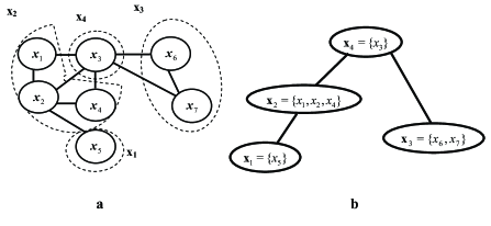
Figure 6: Interaction graph of the DOP with partition (dashed) (a) and quotient interaction graph (b) (example 3).

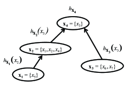
Figure 7: The DAG (generalized elimination tree) of the local block elimination computational procedure for the DO problem (example 3).

A. Forward part

Consider first the block $\mathbf{x_{1}}=\{x_{5}\}$. Then $Nb(\mathbf{x_{1}})=\{x_{2}\}$. Solve using complete enumeration the following optimization problem

$$h_{\mathbf{x_{1}}}(Nb(\mathbf{x_{1}}))=\max_{x_{5}}f_{3}(x_{2},x_{5}),$$

and store the optimal local solutions $\mathbf{x_{1}}$ as a function of a neighborhood, i.e., $\mathbf{x_{1}}^{*}(Nb(\mathbf{x_{1}}))$.

Eliminate the block $\mathbf{x_{1}}$ and consider the block $\mathbf{x_{2}}=\{x_{1},x_{2},x_{4}\}$. $Nb(\mathbf{x_{2}})=\{x_{3}\}$. Now the problem to be solved is

$$h_{\mathbf{x_{2}}}(x_{3})=\max_{x_{1},x_{2},x_{4}}\{h_{\mathbf{x_{1}}}(x_{2})+f_{1}(x_{1},x_{2},x_{3})+f_{2}(x_{2},x_{3},x_{4})\}.$$

Build the corresponding table 10.

Table 9.

Calculation of $h_{\mathbf{x_{1}}}(x_{2})$
$x_{2}$ $h_{\mathbf{x_{1}}}(x_{2})$ $x_{5}^{*}$ 0 6 0 1 5 1

Table 10.

Calculation of $h_{\mathbf{x_{2}}}(x_{3})$
$x_{3}$ $h_{\mathbf{x_{2}}}(x_{3})$ $x_{1}^{*}$ $x_{2}^{*}$ $x_{4}^{*}$ 0 14 1 0 0 1 14 0 0 0

Eliminate the block $\mathbf{x_{2}}$ and consider the block $\mathbf{x_{3}}=\{x_{6},x_{7}\}$. The neighbor of $\mathbf{x_{3}}$ is $x_{3}$: $Nb(\mathbf{x_{3}})=\{x_{3}\}$. Solve the DOP containing $x_{3}$:

$$h_{\mathbf{x_{3}}}(x_{3})=\max_{x_{6},x_{7}}\{f_{4}(x_{3},x_{6},x_{7}),x_{j}\in\{0,1\}\}$$

and build the table 11.

Table 11.

Calculation of $h_{\mathbf{x_{3}}}(x_{3})$
$x_{3}$ $h_{\mathbf{x_{3}}}(x_{3})$ $x_{6}^{*}$ $x_{7}^{*}$ 0 5 0 0 1 6 0 1

Eliminate the block $\mathbf{x_{3}}$ and consider the block $\mathbf{x_{4}}=\{x_{3}\}$. $Nb(\mathbf{x_{4}})=\emptyset$. Solve the DOP:

$$h_{\mathbf{x_{4}}}=\max_{x_{3}}\{h_{\mathbf{x_{2}}}(x_{3})+h_{\mathbf{x_{3}}}(x_{3}),x_{j}\in\{0,1\}\}=20,$$

where $x_{3}^{*}=1$.

B. Backward part.

Consecutively find $\mathbf{x_{3}}^{*},\mathbf{x_{2}}^{*},\mathbf{x_{1}}^{*}$, i.e., the optimal local solutions from the stored tables 11, 10, 9:
$x_{3}^{*}=1\Rightarrow x_{6}^{*}=1,~{}x_{7}^{*}=1$ (table 11);
$x_{3}^{*}=1\Rightarrow x_{1}^{*}=0,~{}x_{2}^{*}=0,~{}x_{4}^{*}=0$ (table 10); $x_{2}^{*}=0\Rightarrow x_{5}^{*}=0$ (table 9).
We found the optimal solution to be $(0,~{}0,~{}1,~{}0,~{}0,~{}1,~{}1)$, the maximum objective value is 20.

Example 4

Local block elimination for constrained DOP

Consider the DOP from example 2 and an ordered partition of the variables of the set into blocks:

$$\mathbf{x_{1}}=\{x_{5}\},~{}\mathbf{x_{2}}=\{x_{1},x_{2},x_{4}\},~{}\mathbf{x_{3}}=\{x_{6},x_{7}\},~{}\mathbf{x_{4}}=\{x_{3}\}.$$

For the ordered partition $\{\mathbf{x_{1}},~{}\mathbf{x_{2}},~{}\mathbf{x_{3}},~{}\mathbf{x_{4}}\}$, this constrained optimization problem may be solved by the LEA.

A. Forward part

Consider first the block $\mathbf{x_{1}}=\{x_{5}\}$. Then $Nb(\mathbf{x_{1}})=\{x_{2}\}$. Solve the following problem containing $x_{5}$ in the objective and the constraints:

$$h_{\mathbf{x_{1}}}(Nb(\mathbf{x_{1}}))=\max_{x_{5}}\{4x_{5}\mid 2x_{2}+3x_{5}\leq 4,x_{j}\in\{0,1\}\}$$

and store the optimal local solutions $\mathbf{x_{1}}$ as a function of a neighborhood, i.e., $\mathbf{x_{1}}^{*}(Nb(\mathbf{x_{1}}))$. Eliminate the block $\mathbf{x_{1}}$. and consider the block $\mathbf{x_{2}}=\{x_{1},x_{2},x_{4}\}$. $Nb(\mathbf{x_{2}})=\{x_{3}\}$. Now the problem to be solved is

$$h_{\mathbf{x_{2}}}(x_{3})=\max_{x_{1},x_{2},x_{4}}\{h_{\mathbf{x_{1}}}(x_{2})+2x_{1}+3x_{2}+5x_{4}\}$$

subject to

$$~{}~{}~{}3x_{1}+4x_{2}+~{}x_{3}~{}~{}~{}~{}~{}~{}~{}~{}~{}~{}\leq 6,$$

$$~{}~{}~{}~{}~{}~{}~{}~{}~{}~{}~{}~{}2x_{2}+3x_{3}+3x_{4}~{}\leq 5,$$

$$~{}~{}~{}~{}~{}~{}~{}~{}~{}~{}~{}~{}~{}~{}~{}~{}~{}~{}~{}~{}~{}~{}~{}x_{j}=0,1,~{}j=1,2,3,4.~{}~{}~{}~{}~{}~{}~{}~{}~{}~{}~{}~{}~{}~{}~{}~{}~{}~{}~{}~{}~{}~{}~{}~{}~{}~{}~{}~{}~{}~{}~{}~{}$$

Build the corresponding table 13.

Table 12.

Calculation of $h_{\mathbf{x_{1}}}(x_{2})$
$x_{2}$ $h_{\mathbf{x_{1}}}(x_{2})$ $x_{5}^{*}$ 0 4 1 1 0 0

Table 13.

Calculation of $h_{\mathbf{x_{2}}}(x_{3})$
$x_{3}$ $h_{\mathbf{x_{2}}}(x_{3})$ $x_{1}^{*}$ $x_{2}^{*}$ $x_{4}^{*}$ 0 11 1 0 1 1 6 1 0 0

Eliminate the block $\mathbf{x_{2}}$ and consider the block $\mathbf{x_{3}}=\{x_{6},x_{7}\}$. The neighbor of $\mathbf{x_{3}}$ is $x_{3}$: $Nb(\mathbf{x_{3}})=\{x_{3}\}$. Solve the DOP containing $x_{3}$:
$h_{\mathbf{x_{3}}}(x_{3})=\max_{x_{6},x_{7}}\{h_{\mathbf{x_{2}}}+x_{3}+6x_{6}+x_{7}~{}|~{}2x_{3}+3x_{6}+2x_{7}\leq 5,x_{j}\in\{0,1\}\}$
and build the table 14.

Table 14.

Calculation of $h_{\mathbf{x_{3}}}(x_{3})$
$x_{3}$ $h_{\mathbf{x_{3}}}(x_{3})$ $x_{6}^{*}$ $x_{7}^{*}$ 0 18 1 1 1 12 1 0

Eliminate the block $\mathbf{x_{3}}$ and consider the block $\mathbf{x_{4}}=\{x_{3}\}$. $Nb(\mathbf{x_{4}})=\emptyset$. Solve the DOP:

$$h_{\mathbf{x_{4}}}=\max_{x_{3}}\{h_{\mathbf{x_{3}}}(x_{3}),x_{j}\in\{0,1\}\}=18,$$

where $x_{3}^{*}=0$.

B. Backward part.

Consecutively find $\mathbf{x_{3}}^{*},\mathbf{x_{2}}^{*},\mathbf{x_{1}}^{*}$, i.e., the optimal local solutions from the stored tables 14, 13, 12. $x_{3}^{*}=0\Rightarrow x_{6}^{*}=1,~{}x_{7}^{*}=1$ (table 14); $x_{3}^{*}=0\Rightarrow x_{1}^{*}=1,~{}x_{2}^{*}=0,~{}x_{4}^{*}=1$ (table 13); $x_{2}^{*}=0\Rightarrow x_{5}^{*}=1$ (table 12). We found the optimal global solution to be $(1,~{}0,~{}0,~{}1,~{}1,~{}1,~{}1)$, the maximum objective value is 18.

6 Tree structural decompositions in discrete optimization

Tree structural decomposition methods use partitioning of constraints and use as a meta-tree a structural graph . Dynamic programming algorithm starts at the leaves of the meta-tree and proceeds from the smaller to the larger subproblems (corresponding to the subtrees) that is to say, bottom-up in the rooted tree.

6.1 Tree decomposition and methods of its computing

Aforementioned facts and an observation that many optimization problems which are hard to solve on general graphs are easy on trees make detection of tree structures in a graph a very promising solution. It can be done with such powerful tool of the algorithmic graph theory as a tree decomposition and the treewidth as a measure for the ”tree-likeness” of the graph RobSey . It is worth noting that in Hlin08 is discussed a number of other useful parameters like branch-width, rank-width (clique-width) or hypertree-width.

Definition 5

Let $G=(X,E)$ be a graph. A tree decomposition of $G$ is a pair $(T;\mathbf{Y})$ with $T=(I;F)$ a tree and $\mathbf{Y}=\{\mathbf{y_{i}}\mid I\in I\}$ a family of subsets of $X$, one for each node of $T$, such that

• (i) $\bigcup_{i\in I}\mathbf{y_{i}}=X,$

• (ii) for every edge $(x,y)\in X$ there is an $i\in I$ with $x\in\mathbf{y_{i}},~{}y\in\mathbf{y_{i}}$,

• (iii) (intersection property) for all $i,j,l\in I$, if $i<j<l$, then $\mathbf{y_{i}}\cap\mathbf{y_{l}}\subseteq\mathbf{y_{j}}$.

Note that tree decomposition uses partition of constraints, i.e., it can be considered as a dual structural decomposition method. The best known complexity bounds are given by the ”treewidth” $tw$ (Robertson, Seymour RobSey ) of an interaction graph associated with a DOP. This parameter is related to some topological properties of the interaction graph. Tree decomposition and the treewidth (Robertson, Seymour RobSey ) play a very important role in algorithms, for many $NP$-complete problems on graphs that are otherwise intractable become polynomial time solvable when these graphs have a tree decomposition with restricted maximal size of cliques (or have a bounded treewidth Arn91 , Bodl97 , BodKos07 ). It leads to a time complexity in $O(n\cdot 2^{tw+1})$. Tree decomposition methods aim to merge variables such that the meta-graph is a tree of meta-vertices.

The procedure to solve a DO problem with bounded treewidth involves two steps: (1) computation of a good tree decomposition, and (2) application of a dynamic programming algorithm that solves instances of bounded treewidth in polynomial time.

Thus, a tree decomposition algorithm can be applied to solving DOPs using the following steps:

1. generate the interaction graph for a DOP (P);

2. using an ordering for Elimination Game add edges in the interaction graph to produce a (chordal) filled graph;

3. build the elimination tree and information flows (see Fig 4(b));

4. identify the maximum cliques, apply an absorption and build subproblems;

5. produce a tree decomposition;

6. solve the DO subproblems for each meta-node and combine the results using LEA.

As finding an optimal tree decomposition is $NP$-hard, approximate optimal tree decompositions using triangulation of a given graph are often exploited. Let us list existing methods of computing tree decomposition using a survey of them in Jegou_comp . Optimal triangulations algorithms have an exponential time complexity. Unfortunately, their implementations do not have much interest from a practical viewpoint. For example, the algorithm described in FomKT04 has time complexity $O(n^{4}\cdot(1.9601^{n}))$ Jegou_comp . A paper GoDech04 has shown that the algorithm proposed in ShoiGei97 cannot solve small graphs (50 vertices and 100 edges). The approach of GoDech04 using a branch and bound algorithm, seems promising for computing optimal triangulations. Approximation algorithms approximate the optimum by a constant factor. Although their complexity is often polynomial in the treewidth Amir , this approach seems unusable due to a big hidden constant. Minimal triangulation computes a set $C^{{}^{\prime}}$ such that, for every subset $C^{{}^{\prime\prime}}\subset C^{{}^{\prime}}$, the graph $G^{{}^{\prime}}=(X,C\cup C^{{}^{\prime\prime}})$ is not triangulated. The algorithms LEX-M RoTaLu76 and LB Berry99 have a polynomial time complexity of $O(ne^{{}^{\prime}})$ with $e^{{}^{\prime}}$ the number of edges in the triangulated graph. Heuristic triangulation methods build a perfect elimination order by adding some edges to the initial graph. They can be easily implemented and often do this work in polynomial time without providing any minimality warranty. In practice, these heuristics compute triangulations reasonably close to the optimum Kjaerulff90 .
Experimental comparative study of four triangulation algorithms, LEX-M, LB, min-fill and MCS was done in Jegou_comp . Min-fill orders the vertices from $1$ to $n$ by choosing the vertex which leads to add a minimum number of edges when completing the subgraph induced by its unnumbered neighbors. Paper Jegou_comp claims that LB and min-fill obtain the best results.

6.2 Computing tree decompositions for NSDP schemes

Given a triangulated (or chordal) graph, the set of its maximal cliques corresponds to the family of subsets associated with a tree decomposition (so called clique tree Blair93 ). When we exploit tree decomposition, we only consider approximations of optimal triangulations by clique trees. Hence, the time complexity is then $O(n\cdot 2^{w^{+}+1})$ ($w+1\leq w^{+}+1\leq n$). The space complexity is $O(n\cdot s\cdot 2^{s})$ with $s$ the size of the largest minimal separator Jegou_comp .
Usually, tree decomposition is considered in the literature separately from NSDP issues. But there is a close connection between these two structural decomposition approaches. Moreover, it is easy to see that a tree decomposition can be obtained from the DAG of the computational NSDP procedure (this fact was noted in KaDeLaDe05 ).

Consider example 2 and build a tree decomposition associated with the corresponding NSDP procedure. Associated underlying DAG of NSDP procedure for the variable ordering $\{x_{5},x_{2},x_{1},x_{4},x_{3},x_{6},x_{7}\}$ is shown in Fig. 4 (b). As was mentioned above, this underlying DAG of local variable elimination (the elimination tree) is constructed using Elimination Game. A node $i$ of the DAG is containing variables $(\alpha_{i},Nb_{G_{x_{i-1}}}^{(i-1)}(x_{i}))$ is linked with the first $x_{j}$ (accordingly to the ordering $\alpha$) which is in $Nb_{G_{x_{i-1}}^{(i-1)}}(x_{i})$. Nodes and edges of desired tree decomposition correspond one-by-one to nodes and edges of the underlying DAG. Each node of the tree decomposition is indeed a meta-node containing a subset of vertices of the interaction graph $G$. This subset induces a subgraph in $G$ that was condensed to generate the meta-node. Restore these subgraphs for each meta-node of the tree decomposition.

Proposition 1

Graph structure obtained by this construction from the underlying DAG of the NSDP procedure is a tree decomposition.

Proof is in KaDeLaDe05 .
In our example 2, we observe that the first (accordingly to ordering $\alpha$) meta-node corresponds to the variable $x_{5}$ and contains variables (vertices) $x_{2},x_{5}$ (i.e., $x_{5}\cup Nb(x_{5})$). Subgraph induced by these vertices can be constructed using the interaction graph $G$ (Fig. 4 a). This subgraph is shown in Fig. 8 (a) — the meta-node $\mathbf{y_{1}}$. Next meta-node $\mathbf{y_{2}}$ of the tree decomposition corresponds to the variable $x_{2}$ and contains variables $x_{1},~{}x_{2},~{}x_{3},~{}x_{4}$. The corresponding induced subgraph (clique) is shown inside the meta-node $\mathbf{y_{2}}$ in Fig. 9 (a). Continuing in analogous way we obtain the tree decomposition as shown in Fig. 8 (a).
It is easy to see that some cliques in this tree decomposition are not maximal and can be absorbed by other cliques. In the case, when one clique contains another clique, the second clique can be absorbed into the first one. Thus, the clique corresponding to the meta-node $\mathbf{y_{2}}$ is absorbed by clique $\mathbf{y_{3}}$ (we denote a result of absorption as a clique $\mathbf{y_{2,3}}$. The clique $\mathbf{y_{5}}$ is absorbed by clique $\mathbf{y_{4}}$ forming a clique $\mathbf{y_{4,5}}$. After absorptions done we obtain a clique tree (Fig. 8 (b)) containing only maximal cliques. These maximal cliques correspond to constraints of the DOP. In Fig. 8 (b) maximal cliques and links between them are shown. Local decomposition algorithm Shch83 that uses a dynamic programming paradigm can be applied to this clique tree. Other possible way of finding the clique tree is using maximal spanning tree in the dual graph.

6.3 Applying the local decomposition algorithm to solving DO problem

To describe how tree decompositions are used to solve problems with the local decomposition algorithm, let us assume we find a tree decomposition of a graph $G$. Since this tree decomposition is represented as a rooted tree $T$, the ancestor/descendant relation is well-defined. We can associate to each meta-node $\mathbf{y}$ the subgraph of $G$ made up by the vertices in $\mathbf{y}$ and all its descendants, and all the edges between those vertices. Starting at the leaves of the tree $T$, one computes information typically stored in a table, in a bottom-up manner for each bag until we reach the root. This information is sufficient to solve the subproblem for the corresponding subgraph. To compute the table for a node of the tree decomposition, we only need the information stored in the tables of the children (i.e. direct descendants) of this node. The DO problem for the entire graph can then be solved with the information stored in the table of the root of $T$. Consider example 2 and exploit the tree decomposition (clique tree) shown in Fig. 8 (b). Let us solve the subproblem corresponding to the block $\mathbf{y_{1}}$. Since this block is adjacent to the block $\mathbf{y_{2,3}}$, we have to solve a DOP with variables $\mathbf{y_{1}}-\mathbf{y_{2,3}}$ for all possible assignments $\mathbf{y_{1}}\bigcap\mathbf{y_{2,3}}$. Thus, since $\mathbf{y_{1}}-\mathbf{y_{2,3}}=\left\{x_{5}\right\}$ and $\mathbf{y_{1}}\bigcap\mathbf{y_{2,3}}=\left\{x_{2}\right\}$, then induced subproblem has the form:

$$h_{\mathbf{y_{1}}}(x_{2})=\max_{x_{5}}\left\{4x_{5}\right\}$$

subject to

$$2x_{2}+3x_{5}\leq 4,~{}~{}x_{j}=0,1,~{}j\in\left\{2,5\right\}$$

Solution of the problem can be written in a tabular form (see table 15).

Table 15.

Calculation of $h_{\mathbf{y_{1}}}(x_{2})$

$x_{2}$	$h_{\mathbf{y_{1}}}$	$x_{5}^{*}(x_{2})$
0	4	1
1	0	0

Table 16.

Calculation of $h_{\mathbf{y_{2,3}}}(x_{3})$

$x_{3}$	$h_{\mathbf{y_{2,3}}}$	$x_{1}^{*}(x_{3})$	$x_{2}^{*}(x_{3})$	$x_{4}^{*}(x_{3})$
0	11	1	0	1
1	6	1	0	0

Since $\mathbf{y_{2,3}}-\mathbf{y_{4}}=\left\{x_{1},x_{2},x_{3},x_{4}\right\}-\left\{x_{3},x_{6},x_{7}\right\}=\left\{x_{1},x_{2},x_{4}\right\}$ and $\mathbf{y_{2,3}}\bigcap\mathbf{y_{4}}=\left\{x_{3}\right\}$, next subproblem corresponding to the leaf (or meta-node) $\mathbf{y_{2,3}}$ of the clique tree is

(a)

(b)

Fig. 8. Tree decomposition for the NSDP procedure (example 2) before (a) and after absorption (b).

$$h_{\mathbf{y_{2,3}}}(x_{3})=\max_{x_{1},x_{2},x_{4}}\left\{h_{\mathbf{y_{1}}}+2x_{1}+3x_{2}+5x_{4}\right\}$$

subject to

$$3x_{1}+4x_{2}+x_{3}\leq 6,~{}~{}2x_{2}+3x_{3}+3x_{4}\leq 5,~{}~{}x_{j}=0,1,~{}j\in\left\{1,2,3,4\right\}$$

Solution of this subproblem is in table 16. The last problem corresponding to the block $\mathbf{y_{4,5}}$ left to be solved is:

$$h_{\mathbf{y_{4,5}}}=\max_{x_{3},x_{6},x_{7}}\left\{h_{\mathbf{y_{2,3}}}(x_{3})+x_{3}+6x_{6}+x_{7}\right\}$$

s.t.

$$2x_{3}+3x_{6}+2x_{7}\leq 5,~{}~{}x_{j}=0,1,~{}j\in\left\{3,6,7\right\}$$

Table 17. Calculation of $h_{\mathbf{y_{4,5}}}$

$h_{\mathbf{y_{4,5}}}$	$x_{3}^{*}$	$x_{6}^{*}$	$x_{7}^{*}$
18	0	1	1

The maximal objective value is 18. To find the optimal values of the variables, it is necessary to do a backward step of the dynamic programming procedure: from table 17 we have $x_{3}^{*}=0,~{}x_{6}^{*}=1,~{}x_{7}^{*}=1$. From the table 16 using the information $x_{3}^{*}=0$ we find $x_{1}^{*}=1,~{}x_{2}^{*}=0,~{}x_{4}^{*}=1$. Considering table 15 we have for $x_{2}^{*}$=0: $x_{5}^{*}=1$. The solution is (1, 0, 0, 1, 1, 1, 1); the maximal objective value is 18.

7 Conclusion

This paper reviews the main graph-based local elimination algorithms for solving DO problems. The main aim of this paper is to unify and clarify the notation and algorithms of various structural DO decomposition approaches. We hope that this will allow us to apply the aforementioned decomposition techniques to develop competitive algorithms which will be able to solve practical real-life discrete optimization problems.

References

- (1) Amestoy PR, Davis TA, Duff IS (1996) An approximate minimum degree ordering algorithm. SIAM J on Matrix Analysis and Applications 17:886–905
- (2) Amir E (2001) Efficient approximation for triangulation of minimum treewidth. In: Proceedings of UAI
- (3) Aris R (1961) The optimal design of chemical reactors. Academic Press, New York
- (4) Arnborg S (1985) Efficient algorithms for combinatorial problems on graphs with bounded decomposability — A survey. BIT 25:2 -23
- (5) Arnborg S, Corneil DG, Proskurowski A (1987) Complexity of finding embeddings in a -tree. SIAM J Alg Disc Meth 8(2):277–284
- (6) Arnborg S, Lagergren J, Seese D (1991) Easy problems for tree-decomposable graphs. J of Algorithms 12:308–340
- (7) Ashcraft C (1995) Compressed graphs and the minimum degree algorithm. SIAM J Sci Comput 16(6):1404–1411
- (8) Ashcraft C, Liu JWH (1995) Robust ordering of sparse matrices using multisection. SIAM J Matrix Anal Appl 19(3):816–832
- (9) Barnhart C, Johnson EL, Nemhauser GL, Savelsbergh MWP, Vance PH (1998) Branch and price: Column generation for solving huge integer programs. Operations Research 46:316–329
- (10) Beeri C, Fagin R, Maier D, Yannakakis M (1983) On the desirability of acyclic database schemes. Journal ACM 30:479 -513
- (11) Beightler CS, Johnson DB (1965) Superposition in branching allocation problems. Journal of Mathematical Analysis and Applications 12:65–70
- (12) Bellman R, Dreyfus S (1962) Applied Dynamic Programming. Princeton University Press, Princeton
- (13) Benders JF (1962) Partitioning procedures for solving mixed-variables programming problems. Numerische Mathematik 4:238–252
- (14) Bertele U, Brioschi F (1969) A new algorithm for the solution of the secondary optimization problem in nonserial dynamic programming. Journal of Mathematical Analysis and Applications 27:565–574
- (15) Bertele U, Brioschi F (1969) Contribution to nonserial dynamic programming. Journal of Mathematical Analysis and Applications 28:313–325
- (16) Bertele U, Brioschi F (1972) Nonserial Dynamic Programming. Academic Press, New York
- (17) Berry A (1999) A wide-range efficient algorithm for minimal triangulation. In: Proceedings of SODA.
- (18) Blair JRS, Peyton B (1993) An introduction to chordal graphs and clique trees. In: Graph theory and sparse matrix computation. Springer, New York
- (19) Bodlaender HL(ed)(2003) Graph-theoretic concepts in computer science. 29th international workshop, WG 2003, Elspeet, The Netherlands, June 19–21, 2003. Lecture Notes in Computer Science 2880. Springer, Berlin
- (20) Bodlaender HL (1997) Treewidth: Algorithmic techniques and results. In: Privara L et al.(eds) Mathematical foundations of computer science. 22nd international symposium, MFCS ’97, Bratislava, Slovakia, August 25-29, 1997. Proceedings. Lect. Notes Comput Sci 1295. Springer, Berlin
- (21) Bodlaender H, Koster AMCA (2008) Combinatorial optimization on graphs of bounded treewidth, Computer Journal 51:255–269
- (22) Burkard RE, Hamacher HW, Tind J (1985) On General Decomposition Schemes in Mathematical Programming. Mathematical Programming Studies 24: ”Festschrift on the occasion of the 70 th birthday of George B. Dantzig”, 238–252
- (23) Cook SA (1971) The complexity of theorem-proving procedures. In: Proc 3rd Ann ACM Symp on Theory of Computing Machinery. New York.
- (24) Cook W, Seymour PD (2003) Tour merging via branch-decomposition. INFORMS Journal on Computing 15:233–248
- (25) Courcelle B (1990) The monadic second-order logic of graphs I: Recognizable sets of finite graphs. Information and Computation 85:12–75
- (26) Crama Y, Hansen P, Jaumard B (1990) The basic algorithm for pseudo-boolean programming revisited, Discrete Applied Mathematics 29:171–185
- (27) Dantzig GB (1949) Programming of interdependent activities II: Mathematical model. Econometrica 17:200–211
- (28) Dantzig GB (1981) Time-staged methods in linear programming. Comments and early history. In: Dantzig GB et al. (eds), Large-Scale Linear Programming, IIASA, Laxenburg, Austria, 3–16
- (29) Dantzig GB (1973) Solving staircase linear programs by a nested block-angular method. Technical Report 73-1. Stanford Univ., Dept. of Operations Research, Stanford
- (30) Dasgupta S, Papadimitriou CH, Vazirani UV (2006) Algorithms. McGraw Hill
- (31) Dechter R (1992) Constraint networks. In: Encyclopedia of Artificial Intelligence, 2nd edn. Wiley, New York
- (32) Dechter R (1999) Bucket elimination: A unifying framework for reasoning. Artificial Intelligence 113:41–85
- (33) Dechter R, El Fattah Y (2001) Topological parameters for time-space tradeoff. Artificial Intelligence 125:93–118
- (34) Dechter R (2003) Constraint processing. Morgan Kaufmann, 2003
- (35) Dechter R, Pearl J (1989) Tree clustering for constraint networks. Artificial Intelligence 38:353–366
- (36) Dolgui A, Soldek J, Zaikin O (eds) (2005) Supply chain optimisation: product/process design, facilities location and flow control. Series: Applied Optimization, XVI. Springer, V. 94
- (37) Esogbue AO, Marks B (l974) Non-serial dynamic programming – A survey. Operational Research Quarterly 25:253–265
- (38) Fernandez-Baca D (1988) Nonserial dynamic programming formulations of satisfiability. Information Processing Letters 27:323–326
- (39) Finkel’shtein YuYu (1965) On solving discrete programming problems of special form (Russian). Economics and Mathematical Methods 1:262–270
- (40) Floudas CA (1995) Nonlinear and mixed-integer optimization: fundamentals and applications. Oxford University Press, Oxford
- (41) Fomin F, Kratsch D, Todinca I (2004) Exact (exponential) algorithms for treewidth and minimum fill-in. In: Proceedings of ICALP
- (42) Fourer R (1984). Staircase matrices and systems. SIAM Review 26(1):1–70
- (43) Freuder E (1992) Constraint solving techniques. In: Tyngu E, Mayoh B, Penjaen J (eds) Constraint Programming of series F: Computer and System Sciences, 51–74. NATO ASI Series
- (44) Fulkerson DR, Gross OA (1965) Incidence matrices and interval graphs. Pacific J of Mathematics 15:835–855
- (45) George JA, Liu JWH (1981) Computer Solution of Large Sparse Positive Definite Systems. Prentice-Hall Inc., Englewood Cliffs
- (46) Gogate V, Dechter R (2004) A complete anytime algorithm for treewidth. In: Proceedings of UAI
- (47) Gottlob G, Leone N, Scarcello F (2000) A comparison of structural CSP decomposition methods. Artificial Intelligence 124:243–282
- (48) Gottlob G, Szeider S (2008) Fixed-parameter algorithms for artificial intelligence, constraint satisfaction and database problems. The Computer Journal 51:303–325
- (49) Gyssens M, Jeavons PG, Cohen DA (1994) Decomposing constraint satisfaction problems using database techniques. Artificial Intelligence 66:57–89
- (50) Gu J, Purdom PW, Franco J, Wah BW (1997) Algorithms for the satisfiability (SAT) problem: A survey. In: Satisfiability Problem Theory and Applications
- (51) Harary F, Norman RZ, Cartwright D (1965) Structural Models: An Introduction to the Theory of Directed Graphs. John Wiley & Sons.
- (52) Hammer PL, Rudeanu S (1968) Boolean Methods in Operations Research and Related Areas, Springer, Berlin Heidelberg New York
- (53) Heggernes P, Eisenstat SC, Kumfert G, Pothen A (2001) The Computational Complexity of the Minimum Degree Algorithm. Techn. report UCRL-ID-148375. Lawrence Livermore National Laboratory. URL: http://www.llnl.gov/tid/lof/documents/pdf/241278.pdf
- (54) Hendrickson B, Rothberg E (1998) Improving the run time and quality of nested dissection ordering. SIAM J. Sci. Comput. 20(2):468–489
- (55) Hicks IV, Koster AMCA, Kolotoglu E (2005). Branch and tree decomposition techniques for discrete optimization. In: Tutorials in Operations Research. INFORMS, New Orleans URL: http://ie.tamu.edu/People/faculty/Hicks/bwtw.pdf.
- (56) Hliněný P, Oum S, Seese D, and Gottlob G (2008) Width parameters beyond tree-width and their applications. The Computer Journal 51:326–362
- (57) Ho JK, Loute E (1981) A set of staircase linear programming test problems. Mathematical Programming 20:245–250
- (58) Hooker JN (2000) Logic-based Methods for Optimization: Combining Optimization and Constraint Satisfaction. John Wiley & Sons, Chichester
- (59) Hooker JN (2002) Logic, optimization and constraint programming. INFORMS Journal on Computing 14:295–321
- (60) Jeavons PG, Gyssens M, Cohen DA (1994) Decomposing constraint satisfaction problems using database techniques. Artificial Intelligence 66:57–89
- (61) Jégou P, Ndiaye SN, Terrioux C (2005) Computing and exploiting tree-decompositions for (Max-)CSP. In: Proceedings of the 11th International Conference on Principles and Practice of Constraint Programming (CP-2005)
- (62) Jensen FV, Lauritzen SL, Olesen KG (1990) Bayesian updating in causal probabilistic networks by local computations. Computat. Statist. Quart. 4:269–282
- (63) Kask K, Dechter R, Larrosa J, Dechter A (2005). Unifying cluster-tree decompositions for reasoning in graphical models. Artificial Intelligence 160:165–193
- (64) Kjaerulff U (1990) Triangulation of graphs – algorithms giving small total state space. Techn.report. Aalborg, Denmark
- (65) Koster AMCA, van Hoesel CPM, Kolen AWJ (1999) Solving frequency assignment problems via tree-decomposition. In: Broersma HJ et al.(Eds). 6th Twente workshop on graphs and combinatorial optimization. Univ. of Twente, Enschede, Netherlands
- (66) Lauritzen SL, Spiegelhalter DJ (1988) Local computation with probabilities on graphical structures and their application to expert systems. J Roy Statist Soc Ser B 50:157–224
- (67) Liu JWH (1990) The role of elimination trees in sparse factorization. SIAM Journal on Matrix Analysis and Applications 11:134–172
- (68) Martelli A, Montanari U (1972) Nonserial Dynamic Programming: On the Optimal Strategy of Variable Elimination for the Rectangular Lattice. Journal of Mathematical Analysis and Applications 4O:226–242
- (69) Mitten LG, Nemhauser GL (1963) Multistage optimization. Chemical Engineering Progress 54:52–60
- (70) Karypis G, Kumar V (1998) MeTiS - a software package for partitioning unstructured graphs, partitioning meshes, and computing fill-reducing orderings of sparse matrices. Version 4, University of Minnesota. URL: http://www-users.cs.umn.edu/ karypis/metis.
- (71) Mitten LG, Nemhauser GL (1963) Multistage optimization. Chemical Engineering Progress 54:52–60
- (72) Neapolitan RE (1990) Probabilistic Reasoning in Expert Systems. Wiley, New York
- (73) Nemhauser GL, Wolsey LA (1988) Integer and Combinatorial Optimization. John Wiley & Sons, Chichester
- (74) Nemhauser GL (1994) The age of optimization: solving large-scale real-world problems. Operations Research 42:5–13
- (75) Nowak I (2005) Lagrangian decomposition of block-separable mixed-integer all-quadratic programs. Mathematical Programming 102:295–312
- (76) Neumaier A, Shcherbina O (2008) Nonserial dynamic programming and local decomposition algorithms in discrete programming (submitted). URL: http://www.optimization-online.org/DB_HTML/2006/03/1351.html
- (77) Pang W, Goodwin SD (1996) A new synthesis algorithm for solving CSPs. In: Proc of the 2nd Int Workshop on Constraint-Based Reasoning. Key West
- (78) Pardalos PM, Du DZ (eds) (1998) Handbook of combinatorial optimization. Volumes 1, 2, and 3. Kluwer Academic Publishers
- (79) Pardalos PM, Wolkowicz H (eds) (2003) Novel approaches to hard discrete optimization. Fields Institute, American Mathematical Society
- (80) Parter S (1961) The use of linear graphs in Gauss elimination, SIAM Review 3:119–130
- (81) Pearl J (1988) Probabilistic reasoning in intelligent systems. Morgan Kaufmann, San Mateo, CA
- (82) Ralphs TK, Galati MV (2005) Decomposition in integer linear programming. In: Karlof J (Ed) Integer Programming: Theory and Practice
- (83) Robertson N, Seymour PD (1986) Graph minors. II. Algorithmic aspects of tree width. J of Algorithms 7:309–322
- (84) Rose D, Tarjan R, Lueker G (1976) Algorithmic aspects of vertex elimination on graphs. SIAM J on Computing 5:266–283
- (85) Rose DJ (1972) A graph-theoretic study of the numerical solution of sparse positive definite systems of linear equations. In: Read RC (ed) Graph Theory and Computing, 183–217. Academic Press, New York
- (86) Rosenthal A (1982) Dynamic programming is optimal for nonserial optimization problems. SIAM J Comput 11:47–59
- (87) Seidel P (1981) A new method for solving constraint satisfaction problems. In: Proc. of the 7th IJCAI, 338–342. Vancouver, Canada
- (88) Sergienko IV, Shylo VP (2003) Discrete Optimization: Problems, Methods, Studies. Naukova Dumka, Kiev
- (89) Shcherbina O (1980) A local algorithm for integer optimization problems. USSR Comput Math Math Phys 20:276–279
- (90) Shcherbina OA (1983) On local algorithms of solving discrete optimization problems. Problems of Cybernetics (Moscow) 40:171–200
- (91) Shcherbina O (2007) Nonserial dynamic programming and tree decomposition in discrete optimization. In: Proc. of Int. Conference on Operations Research ”Operations Research 2006”. Karlsruhe, 6-8 September, 2006, 155–160. Springer Verlag, Berlin
- (92) Shcherbina OA (2007) Tree decomposition and discrete optimization problems: A survey. Cybernetics and Systems Analysis 43:549–562
- (93) Shcherbina OA (2007) Methodological issues of dynamic programming. Dynamich Sistemy 22:21–36 (in Russian)
- (94) Shcherbina OA (2008) Local elimination algorithms for solving sparse discrete problems. Comput Math and Math Phys 48:152–167
- (95) Shenoy PP, Shafer G (1986) Propagating belief functions using local computations. IEEE Expert 1:43–52
- (96) Shoikhet K, Geiger D (1997) A practical algorithm for finding optimal triangulation. In: Proceedings of AAAI
- (97) Urrutia J (2007) Local solutions for global problems in wireless networks. J of Discrete Algorithms 5:395–407
- (98) Vanderbeck F, Savelsbergh M (2006) A generic view at the Dantzig-Wolfe decomposition approach in mixed integer programming. Operations Research Letters 34:296–306
- (99) Van Roy TJ (1983) Cross decomposition for mixed integer programming. Mathematical Programming 25:46–63
- (100) Wah BW, Li G-J (1988) Systolic processing for dynamic programming problems. Circuits Systems Signal Process 7:119–149
- (101) Wilde D, Beightler C (1967) Foundations of Optimization. Prentice-Hall, Englewood Cliffs
- (102) Weigel R, Faltings B (1999) Compiling constraint satisfaction problems. Artificial Intelligence 115:257–287
- (103) Wets RJB (1966) Programming under uncertainty: The equivalent convex program. SIAM J Appl Math 14:89–105
- (104) Zhuravlev YuI (1998) Selected Works. Magistr, Moscow (in Russian)
- (105) Zhuravlev YuI, Losev GF (1995) Neighborhoods in problems of discrete mathematics. Cybern Syst Anal 31:183–189