A Unified Approach to High-Gain Adaptive Controllers

Abstract

It has been known for some time that proportional output feedback will stabilize MIMO, minimum-phase, linear time-invariant systems if the feedback gain is sufficiently large. High-gain adaptive controllers achieve stability by automatically driving up the feedback gain monotonically. More recently, it was demonstrated that sample-and-hold implementations of the high-gain adaptive controller also require adaptation of the sampling rate. In this paper, we use recent advances in the mathematical field of dynamic equations on time scales to unify and generalize the discrete and continuous versions of the high-gain adaptive controller. We prove the stability of high-gain adaptive controllers on a wide class of time scales.

Keywords: time scales, hybrid system, adaptive control

1 Introduction

The concept of high-gain adaptive feedback arose from a desire to stabilize certain classes of linear continuous systems without the need to explicitly identify the unknown system parameters. This type of adaptive controller does not identify system parameters at all, but rather adapts the feedback gain itself in order to regulate the system. A number of papers examine the details of various kinds of high-gain adaptive controllers [11, 15, 18, 23], among others. More recently, several papers have discussed one particularly practical angle on the high-gain adaptive controller, namely how to cope with input/output sampling. In particular, Owens [17] showed that it is not generally possible to stabilize a linear system with adaptive high-gain feedback under uniform sampling. Thus, Owens, et. al., develop a mechanism to adapt the sampling rate as well as the gain, a notion subsequently improved upon by Ilchmann and Townley [12, 13, 14], and Logemann [16].

In this paper, we employ results from the burgeoning new field of mathematics called dynamic equations on time scales to accomplish three principal objectives. First, we use time scales to unify the continuous and discrete versions of the high-gain controller, which have previously been treated separately. Next we give an upper bound on the system graininess to guarantee stabilizability for a much wider class of time scales than previously known, including mixed continuous/discrete time scales. Third, the paper represents the first application of several very recent advances in stability theory and Lyapunov theory for systems on time scales, and two new lemmas are presented in that vein. We also give a simulation of a high-gain controller on a mixed time scale.

2 Background

We first state two assumptions that are required in the subsequent text.

(A1)

The system model and feedback law are given by the linear, time-invariant, minimum phase system

$$\dot{x}(t) =Ax(t)+Bu(t),\qquad y(t)=Cx(t),\qquad x(0)=x_{0},$$ (1)

$$u(t) =-k(t)y(t),$$ (2)

for $t\geq 0$. System parameters $A\in\mathbb{R}^{n\times n}$, $B,C^{T}\in\mathbb{R}^{n\times m}$, $x_{0}\in\mathbb{R}^{n}$ and $n$ are unknown. The feedback gain $k:\mathbb{R}\rightarrow\mathbb{R}^{+}$ is piecewise continuous, and nondecreasing as $t\rightarrow\infty$. By minimum phase, we mean that the polynomial

$$\det\begin{bmatrix}A-\lambda I&B\\ C&0\end{bmatrix}$$

with $\lambda\in\mathbb{C}$ is Hurwitz (zeros in open left hand plane).

(A2)

Furthermore,

$$(CB)^{T}+(CB)>0,$$ (3)

i.e. $(CB)^{T}+(CB)$ is positive definite. (In [18] it is pointed out that a nonsingular input/output transformation  $T$ always exists such that $\tilde{B}=BT^{-1}$ and $\tilde{C}=TC$ give $(\tilde{C}\tilde{B})^{T}+(\tilde{C}\tilde{B})>0$.)

Under these conditions it has been known for some time (e.g. [11]) that there are a wide class of gain adaptation laws $k(t)=f(y(t))$, $f:\mathbb{R}^{m}\rightarrow\mathbb{R}$, that can asymptotically stabilize system (1) in the sense that

$$y\in L^{2}[t_{0},\infty),\qquad\lim_{t\rightarrow\infty}k(t)<\infty.$$

Subsequently, various authors [11, 12, 17, 19] assumed that the output is obtained via sample-and-hold, i.e. $y_{i}:=y(t_{i})$ with $k_{i}:=k(t_{i})$ and $i\in\mathbb{N}_{0}$. Thus it becomes necessary also to adapt the sample period $h_{i}:=t_{i+1}-t_{i}$ so the closed-loop control objectives are

$$y_{i}\in\ell^{2}[i_{0},\infty),\qquad\lim_{i\rightarrow\infty}k_{i}<\infty,\qquad\lim_{i\rightarrow\infty}h_{i}>0.$$

Though several variations on these results exist, these remain the basic control results for continuous and discrete high-gain adaptive controllers. The continuous and discrete cases have previously been treated quite differently, but we now construct a common framework for both using time scale theory.

3 A Time Scale Model

The system of (A1) can be replaced by

$$x^{\Delta}(t) =\hat{A}(t)x(t)+\hat{B}(t)u(t),\qquad y(t)=Cx(t),\qquad x(0)=x_{0},$$ (4)

$$u(t) =k(t)y(t),\qquad t\in\mathbb{T},$$ (5)

where $\mathbb{T}$ is any time scale unbounded above with $0\in\mathbb{T}$. With a series expansion similar to [11], we see that

$$\hat{A}(t):=\operatorname{expc}(\mu(t)A)A,\qquad\hat{B}(t)=\operatorname{expc}(\mu(t)A)B,$$ (6)

where expc is the matrix power series function

$$\operatorname{expc}(X):=I+\frac{1}{2}X+\frac{1}{6}X^{2}+\cdots+\frac{1}{n!}X^{n-1}+\cdots$$ (7)

and $\mu$ is the time scale graininess. Implementing control law (2) then gives

$$x^{\Delta}(t)=\mathcal{A}(t)x(t),\qquad\mathcal{A}(t):=\operatorname{expc}(\mu(t)A)(A-k(t)BC).$$ (8)

Note that $\hat{A},\hat{B}$ and $\mathcal{A}$ may all be time-varying, but we will henceforth drop the explicit reference to $t$ for these variables. For future reference, we also note that if $\sup_{t\in\mathbb{T}}\mu(t)<\infty$, then $||\hat{A}||$ and $||\hat{B}||$ are also bounded (c.f. Appendix, Lemma 7.4).

The design objectives are to find graininess $\mu$ and feedback gain $k$ as functions of the output $y$,

$$\mu(t) =g(y(t)),\qquad g:\mathbb{R}^{m}\rightarrow[0,\infty),$$ (9)

$$k(t) =f(y(t)),\qquad f:\mathbb{R}^{m}\rightarrow\mathbb{R}^{+},$$ (10)

with $t\in$ $\mathbb{T}$ and $k\in C_{rd}(\mathbb{T})$ nondecreasing, such that

$$y\in L^{2}[t_{0},\infty)_{\mathbb{T}}:=\left\{w:\int_{t_{0}}^{\infty}|w(t)|^{2}\Delta t<\infty\right\},\qquad\lim_{t\rightarrow\infty}k(t)<\infty.$$

It is important to keep in mind the generality of the expressions above. A great deal of mathematical machinery supports the existence of delta derivatives on arbitrary times scales, as well as the existence and characteristics of solutions to (8). See, for example, e.g. [2, 3].

4 Stability Preliminaries

We begin this section with a definition and theorem from the work of Pötzsche, Siegmund, and Wirth [20]:

Definition 4.1.

The set of exponential stability for the time-varying scalar equation $z^{\Delta}(t)=\lambda(t)z(t)$, $z_{0}:=z(t_{0})\in\mathbb{C}$ with $\lambda:\mathbb{T}\rightarrow\mathbb{C}$ and $z,\lambda\in C_{rd}(\mathbb{T)}$, is given by

$$\mathcal{S}(\mathbb{T}):=\mathcal{S}_{\mathbb{C}}(\mathbb{T})\cup\mathcal{S}_{\mathbb{R}}(\mathbb{T})$$

where

$$\mathcal{S}_{\mathbb{C}}(\mathbb{T}) :=\left\{\eta(t)\in\mathbb{C}:\alpha=-\limsup_{t\rightarrow\infty}\frac{1}{t-t_{0}}\int_{t_{0}}^{t}\frac{\log||1+\mu(t)\eta(t)||}{\mu(t)}\Delta t>0\right\},$$ (11)

$$\mathcal{S}_{\mathbb{R}}(\mathbb{T}) :=\left\{\eta(t)\in\mathbb{R}:\forall t\in\mathbb{T},\exists\tau>t\text{ with }\tau\in\mathbb{T}\text{ such that }1+\mu(t)\eta(t)=0\right\},$$

with $\eta\in C_{rd}(\mathbb{T)}$ and arbitrary $t_{0}\in\mathbb{T}$.

Theorem 4.2.

[20] Solutions of the scalar equation $z^{\Delta}(t)=\lambda(t)z(t)$ are exponentially stable on an arbitrary $\mathbb{T}$ if and only if $\lambda(t)\in\mathcal{S}(\mathbb{T})$.

We note here that Pötzche, Siegmund, and Wirth did not explicitly consider scenarios where $\eta$ is time-varying, but their stability analysis remains unchanged for $\eta(t)$.

The set $\mathcal{S}_{\mathbb{R}}(\mathbb{T})$ contains nonregressive eigenvalues $\lambda(t)$, and a loose interpretation of $\mathcal{S}_{\mathbb{C}}(\mathbb{T})$ suggests that it is necessary for a regressive eigenvalue to reside in the area of the complex plane where $||1+\mu(t)\lambda(t)||<1$ “most” of the time. The contour $||1+\mu(t)\lambda(t)||=1$ is termed the Hilger Circle. Since the solution of $z^{\Delta}(t)=\lambda(t)z(t)$ is $x(t)=z_{0}e_{\lambda}(t,t_{0})$, Theorem 4.2 states that, if $\lambda(t)\in\mathcal{S}(\mathbb{T})$ then some $K(t_{0})>1$ exists such that

$$||z(t)||=||z_{0}||||e_{\lambda}(t,t_{0})||\leq||z_{0}||Ke^{-\alpha(t-t_{0})},$$ (12)

where $e_{\lambda}$ is a generalized time scale exponential. The Hilger Circle will be important in the upcoming Lyapunov analysis, as will the following lemmas.

Lemma 4.3.

Let $z\in C_{rd}(\mathbb{T)}$ be a function which is known to satisfy the inequality $z^{\Delta}(t)\leq\lambda(t)z(t)$, $z(0)=z_{0}\in\mathbb{R}$ with $\lambda:\mathbb{T}\rightarrow\mathbb{R}$ and $\lambda\in C_{rd}(\mathbb{T)}$. If $z(t)>0$ for all $t\geq t_{0}\in\mathbb{T}$, then $\lambda(t)\in\mathcal{R}^{+}$.

Proof.

Defining $v(t)=z^{\Delta}(t)-\lambda(t)z(t)$ gives rise to the initial value problem

$$z^{\Delta}(t)-\lambda(t)z(t)=v(t),\quad z(0)=z_{0},\quad t\in\mathbb{T},$$ (13)

where $v(t)\leq 0$.

First, suppose $\lambda(t)$ is negatively regressive for $t\geq t_{0}$, i.e. $\lambda(t)<-1/\mu(t)$ with $\mu(t)>0$. Then (13) yields $z^{\sigma}=\mu\lambda z+z+\mu v=z(1+\mu\lambda)+\mu v<0$.

On the other hand, suppose $\lambda(T)$ is nonregressive for some $T>t_{0},$ $T\in\mathbb{T}$. If $\lambda(t)<-1/\mu(t)$ over $T>t\geq t_{0}$, then invoke the preceding argument. If $\lambda(t)>-1/\mu(t)$ over $T>t\geq t_{0}$, then solve (13)  to get

$$z(t)=e_{\lambda}(t,t_{0})z_{0}+\int_{t_{0}}^{t}e_{\lambda}(t,\sigma(\tau))v(\tau)\Delta\tau,\qquad T>t\geq t_{0}.$$ (14)

Since $e_{\lambda}(t,t_{0})>0$ for $t<T$, we see that $\int_{t_{0}}^{t}e_{\lambda}(t,\sigma(\tau))v(\tau)\Delta\tau<0$. However, for $t\geq T$, (14) becomes

$$z(t)=0+\int_{t_{0}}^{\rho(T)}e_{\lambda}(t,\sigma(\tau))v(\tau)\Delta\tau,\qquad t\geq T$$ (15)

Thus, $z(t)<0$ for all $t\geq t_{0}$ for both negatively regressive and nonregressive $\lambda(t)$, a contradiction of the Lemma’s presupposition. This leaves only $\lambda(t)\in\mathcal{R}^{+}$. ∎

At this point we pause briefly to discuss Lyapunov theory on time scales. DaCunha produced two pivotal works [5, 6] on solutions $P$ of the generalized time scale Lyapunov equation,

$$A(t)^{T}P(t)+P(t)A(t)+\mu(t)A^{T}(t)P(t)A(t)=-Q(t),\text{ \ \ \ }t\in\mathbb{T},$$ (16)

where $A(t),P(t),Q(t)\in\mathbb{R}^{n\times n}$, $\ A$ and $Q$ are known and $Q(t)>0$. Though it will not be necessary to solve (16) in this work, we will see that the form of (16) leads to an upper bound on the graininess that is generally applicable to MIMO systems, an advancement beyond previous works which gave an explicit bound only for SISO systems.

Before the next lemma, we define

$$\mathcal{K}:=\{k:\mathbb{T\rightarrow\mathbb{R}}^{+},\ k\in C_{rd}(\mathbb{T}),\ k^{\Delta}(t)\geq 0\ \forall t\in\mathbb{T},\ \lim_{t\rightarrow\infty}k(t)=\infty\}.$$

The next lemma follows directly.

Lemma 4.4.

Given assumptions (A1) and (A2) and $k\in\mathcal{K}$, there exists a nonzero graininess $\bar{\mu}(t)$ and a time $t^{\ast}$ such that, for all $\mu(t)\leq\bar{\mu}(t)$ and $t>t^{\ast}$, the matrix $-kC\hat{B}$ satisfies a time scale Lyapunov equation with $P=I$, $Q(t)\geq\varepsilon_{2}$ for small $\varepsilon_{2}>0$, and $\hat{B}$ from (6).

Proof.

We construct $\bar{\mu}(t)$ as

$$\bar{\mu}(t):=\frac{1}{k(t)}\left(\frac{\lambda_{\min}\{CB+(CB)^{T}\}}{\lambda_{\max}\{(CB)^{T}CB\}}-\varepsilon_{1}\right),\qquad t\in\mathbb{T},$$ (17)

with $\varepsilon_{1}>0$ sufficiently small so that $\bar{\mu}(t)>0$ on $\mathbb{T}$. This holds if

$$(CB)^{T}+CB-\bar{\mu}(t)k(t)(CB)^{T}CB=\varepsilon_{1}I.$$ (18)

Multiplying (18) by $-k(t)$ gives

$$(-k(t)CB)^{T}+(-k(t)CB)+\bar{\mu}(t)(-k(t)CB)^{T}(-k(t)CB)=-k(t)\varepsilon_{1}I.$$

(We now drop the explicit time-dependence for readability.) Set

$$\Sigma(\bar{\mu}):=\operatorname{expc}(\bar{\mu}A)-I,$$

so that $\hat{B}(\bar{\mu})=[I+\Sigma(\bar{\mu})]B$, yielding

$$(-kC\hat{B})^{T}+(-kC\hat{B})+\bar{\mu}(-kC\hat{B})^{T}(-kC\hat{B})=-k(\varepsilon_{1}I-Z),$$

where each term of $Z$ is a product of contants times $\Sigma(\bar{\mu})$. Since $||\Sigma(\bar{\mu})||$ $\rightarrow 0$ as $\bar{\mu}\rightarrow 0$ (c.f. Appendix, Lemma 7.4), there exists a time $t^{\ast}\in\mathbb{T}$ when $||Z||<\varepsilon_{1}$. Because the preceding arguments admit any graininess $\mu(t)\leq\bar{\mu}(t)$, it follows that

$$(-kC\hat{B})^{T}+(-kC\hat{B})+\mu(-kC\hat{B})^{T}(-kC\hat{B})=-kQ,\qquad t>t^{\ast},\ \mu(t)\leq\bar{\mu}(t),$$ (19)

where $Q(t)\geq\varepsilon_{2}$ and $\varepsilon_{2}:=\varepsilon_{1}-||Z||>0$. ∎

We comment briefly on the intuitive implication of Lemma 4.4. Equation (19) shows that there exist positive definite $Q(t)$ and $P=I$ to satisfy an equation of the form (16). According to DaCunha, this implies that the eigenvalues of $-kC\hat{B}$ lie strictly within the Hilger circle for $t>t^{\ast}$.

5 System Stability

We now come to the three central theorems of the paper. If $BC$ is not known to be full rank, or cannot be full rank because of the input/output dimensions, then it must be assumed (or determined a priori) that the eigenvalues of $A-k(t)BC$ attain negative real parts at some point in time. This phenomenon is investigated in-depth by other authors [11, 23]. We then make use of the observation by Owens, et. al. [18], that there must exist some $k^{\ast}>0$ such that if $k(t)\equiv k^{\ast}$ the system of (A1) has a positive-real realization. This, together with the Kalman-Yakubovich Lemma [21], implies existence of $P,Q>0$ so that

$$(A-k^{\ast}BC)^{T}P+P(A-k^{\ast}BC)=-Q\quad\text{ and }\quad PB=C^{T}CB.$$ (20)

Theorem 5.1 (Exponential Stability).

In addition to (A1) and (A2), suppose

1. $t\in\mathbb{T}$ where ${\mathbb{T}}$ is a time scale which is unbounded above but with $\mu(t)\leq\bar{\mu}(t)$,

2. $k\in\mathcal{K}$ (implying from (17) that $\mu(t)\rightarrow 0$, but not necessarily monotonically),

3. $BC$ is not necessarily full rank, but there exists a time $t^{\ast}\in\mathbb{T}$ such that the eigenvalues of $(A-k(t)BC)$ are strictly in the left-hand complex plane for $t\geq t^{\ast}$.

Then the system (4), (5) is exponentially stable in the sense that there exists time $t_{0}\in\mathbb{T}$ and constants $K(t_{0})\geq 1$, $\alpha\geq 0$, such that

$$||x(t)||\leq||x(t_{0})||Ke^{-\frac{1}{2}\alpha(t-t_{0})},\qquad t\geq t_{0}.$$

Proof.

Set $k^{\ast}:=k(t^{\ast})$. Then assumption (iii) is the prerequisite for equation (20). Again, we suppress the time-dependence of $x$, $k$, $\mu$, $\hat{A}$ and $\hat{B}$. Similarly to Lemma 4.4, terms containing $\Sigma(\mu)$ may be added to the first equality in (20) to obtain

$$(\hat{A}-k^{\ast}\hat{B}C)^{T}P+P(\hat{A}-k^{\ast}\hat{B}C)\leq-\varepsilon_{3}\qquad t\geq t^{\ast\ast},$$ (21)

for some small $\varepsilon_{3}>0$. Note $t=t^{\ast\ast}$ is the point at which terms involving $\Sigma(\mu)$ become small enough for (21) to hold. Defining $Z_{1}:=C^{T}C\Sigma B-P\Sigma B$, the second equality in (20) gives

$$P\hat{B}=C^{T}C\hat{B}+Z_{1}.$$

Consider the Lyapunov function $V=x(t)^{T}Px(t)$ with $P$ from (20). Then, using (20), (21) and Lemma 4.4,

$$V^{\Delta} =x^{T\Delta}Px+x^{\sigma T}Px^{\Delta}$$

$$=x^{T}[\mathcal{A}^{T}P+P\mathcal{A}+\mu\mathcal{A}^{T}P\mathcal{A}]x$$

$$=x^{T}\left[(\hat{A}-k^{\ast}\hat{B}C)^{T}P+P(\hat{A}-k^{\ast}\hat{B}C)-(k-k^{\ast})(C^{T}\hat{B}^{T}P+P\hat{B}C)\right.$$

$$\qquad\left.+\mu(\hat{A}-k\hat{B}C)^{T}P(\hat{A}-k\hat{B}C)\right]x$$

$$\leq x^{T}[-\varepsilon_{3}-(k-k^{\ast})(C^{T}\hat{B}^{T}C^{T}C+C^{T}C\hat{B}C+2Z_{1}C)$$

$$\qquad+\mu\hat{A}^{T}P\hat{A}-2\mu k\hat{A}^{T}P\hat{B}C+\mu k^{2}C^{T}\hat{B}^{T}C^{T}C\hat{B}C+\mu k^{2}C^{T}\hat{B}^{T}Z_{1}C]x$$

$$=x^{T}[-\varepsilon_{3}+\mu\hat{A}^{T}P\hat{A}]x$$

$$\qquad+y^{T}[-k(C\hat{B})^{T}-kC\hat{B}+\mu k^{2}(C\hat{B})^{T}C\hat{B}+\mu k^{2}\hat{B}^{T}Z_{1}+k^{\ast}((C\hat{B})^{T}+C\hat{B})]y$$

$$\qquad+x^{T}[-(k-k^{\ast})2Z_{1}-2\mu k\hat{A}^{T}P\hat{B}]y$$

$$\leq-(\varepsilon_{3}-\mu||\hat{A}^{T}P\hat{A}||)x^{T}x$$

$$\qquad-(k\varepsilon_{2}-\mu k||\hat{B}||kZ_{1}||-2k^{\ast}||C\hat{B}||)y^{T}y$$

$$\qquad+(2||kZ_{1}||+2\mu k||\hat{A}^{T}P\hat{B}||)x^{T}y.$$

At this point we observe the following:

• $||\hat{A}^{T}P\hat{A}||$ is bounded because $\hat{A}$ is bounded. Set $\gamma_{1}:=\sup_{t\in\mathbb{T}}||\hat{A}^{T}P\hat{A}||.$

• $\mu k$ is bounded by assumption (i) and (17).

• $||kZ_{1}||$ is bounded because $k$ is proportional to $\frac{1}{\mu}$ and $\frac{1}{\mu}||\Sigma(\mu)||\rightarrow const$ as $\mu\rightarrow 0$. Set $\gamma_{2}:=\sup_{t\in\mathbb{T}}2||kZ_{1}||.$

• Set $\gamma_{3}:=\sup_{t\in\mathbb{T}}\mu k||\hat{B}||\gamma_{2}$.

• Set $\gamma_{4}:=\sup_{t\in\mathbb{T}}2k^{\ast}||C\hat{B}||.$

• Set $\gamma_{5}:=\sup_{t\in\mathbb{T}}2\mu k||\hat{A}^{T}P\hat{B}||.$

Recalling the standard inequality $x^{T}y\leq\beta x^{T}x+\frac{1}{\beta}y^{T}y$ for any $\beta>0$, we then have

$$V^{\Delta}\leq-(\varepsilon_{3}-\mu\gamma_{1}-\beta\gamma_{2}-\beta\gamma_{5})x^{T}x-(k\varepsilon_{2}-\gamma_{3}-\gamma_{4}-\frac{1}{\beta}\gamma_{2}-\frac{1}{\beta}\gamma_{5})y^{T}y.$$

By assumption (ii), there exists a time $t_{0}\geq\max\{t^{\ast},t^{\ast\ast}\}$ such that, for sufficiently small $\beta$,

$$V^{\Delta}\leq\frac{-(\varepsilon_{3}-\mu\gamma_{1}-\beta\gamma_{2}-\beta\gamma_{5})}{\gamma_{\min}(P)}V:=\eta(t)V,\qquad t\geq t_{0},$$

with $\eta(t)<0$. Then, by [2, Theorem 6.1], Theorem 4.2, and Lemma 4.3 it follows that there exists $K(t_{0})\geq 1$ so that

$$||x(t)||\leq K||x(t_{0})||e^{-\frac{1}{2}\alpha(t-t_{0})},\qquad t\geq t_{0},$$

where $\alpha$ is defined in (11). ∎

We point out that, when $BC$ is full rank, assumption (iii) above is no longer necessary as there always exists a $k^{\ast}$ such that the eigenvalues of $(A-k(t)BC)$ are strictly real-negative for $k(t)\geq k^{\ast}$. One more lemma is required before the next theorem.

Lemma 5.2.

If $\mathbb{T}$ is a time scale with bounded graininess (i.e. $\mu_{\infty}:=\sup_{t\in\mathbb{T}}\mu(t)<\infty$), then

$$c_{1}\int_{t_{0}}^{\infty}e^{\alpha t}\,dt\leq\int_{t_{0}}^{\infty}e^{\alpha t}\,\Delta t\leq c_{2}\int_{t_{0}}^{\infty}e^{\alpha t}\,dt,$$

where $c_{1}$, $c_{2}$, $\alpha\in\mathbb{R}$ and $c_{1}$, $c_{2}>0$.

Proof.

Consider the case when $\alpha>0$. The process of time scale integration is akin to the approximation of a continuous integral via a left-endpoint sum of (variable width) rectangles. If the function to be summed is increasing (as in this case), the sum of rectangular areas will be less than the continuous integral, meaning $c_{2}=1$, $c_{1}<1$. One estimate of the lower bound, then, follows by simply increasing $c_{1}$ until $c_{1}e^{\alpha t}$ meets one of the rectangle right endpoints which are given by $e^{\alpha\rho(t)}$. Thus $c_{1}e^{\alpha t}\leq e^{\alpha\rho(t)}$, or equivalently, $c_{1}e^{\alpha\sigma(t)}\leq e^{\alpha t}$. This in turn yields $c_{1}\leq e^{-\alpha\mu(t)}$. Therefore, the most conservative bound is given by $c_{1}\leq e^{-\alpha\mu_{\infty}}$. The case for $\alpha<0$ can be argued similarly, leading to the lemma’s conclusion:

$$c_{1}=\begin{cases}e^{-\alpha\mu_{\infty}},&\alpha>0,\\ 1,&\alpha\leq 0,\end{cases}\qquad c_{2}=\begin{cases}1,&\alpha\geq 0,\\ e^{-\alpha\mu_{\infty}},&\alpha<0.\end{cases}$$

∎

We are now in a position to state the main theorem of the paper.

Theorem 5.3.

In addition to (A1) and (A2), assume the prototypical update law, $k^{\Delta}(t)=||y(t)||^{2}$ with $k_{0}:=k(0)>0$. Then $\lim_{t\rightarrow\infty}k(t)<\infty$ and $y\in L_{2}[t_{0},\infty)_{\mathbb{T}}$.

Proof.

For the sake of contradiction, assume $k(t)\rightarrow\infty$ as $t\rightarrow\infty$. Then $k\in\mathcal{K}$. Theorem 5.1 yields $x\in L_{\infty}[t_{0},\infty)_{\mathbb{T}}$ and therefore $y\in L_{\infty}[t_{0},\infty)_{\mathbb{T}}$. The solution for $k(t)$ is (by [2, Theorem 2.77]),

$$k(t)=k(t_{0})+\int_{t_{0}}^{t}||y(\tau)||^{2}\Delta\tau\leq k(t_{0})+||C||^{2}\int_{t_{0}}^{t}||x(\tau)||^{2}\Delta\tau,\qquad t\geq t_{0.}$$

In conjunction with Lemma 5.2, this allows

$$\lim_{t\rightarrow\infty}k(t) \leq k(t_{0})+||C||^{2}\int_{t_{0}}^{\infty}||x(t)||^{2}\,\Delta t$$

$$\leq k(t_{0})+||C||^{2}||x(t_{0})||^{2}K^{2}\int_{t_{0}}^{\infty}e^{-\alpha(t-t_{0})}\,\Delta t$$

$$=k_{0}+||C||^{2}||x(t_{0})||^{2}K^{2}\int_{0}^{\infty}e^{-\alpha t}\,\Delta t$$

$$<\infty.$$

This contradicts the assumption, so it must be that $k(t)<\infty$ for $t\in\mathbb{T}$. It also immediately follows that $\int_{t_{0}}^{\infty}||y||^{2}\Delta t<\infty$. ∎

It seems possible that Theorem 5.3 may be improved to show that the output is convergent, i.e. $y(t)\rightarrow 0$ as $t\rightarrow\infty$. This is left as an open problem.

6 Discussion

We remark here that there is a great amount of freedom in the choice of the update law for $k(t)$ (c.f. [17]). We use the simplest choice for convenience (as do most authors); the essential arguments remain unchanged for other choices. There is also freedom in the choice of update for $\mu(t)$. The expression (18), can be simplified to

$$(CB)^{T}+CB-\mu(t)k(t)(CB)^{T}CB>0,\qquad t\in\mathbb{T},$$

for any $\mu(t)\leq\bar{\mu}(t)$. In the SISO case, this further reduces to the expression derived by Owens [17], that $\mu kCB<2$. It requires the graininess (which may interpreted as the system sampling step size for sample-and-hold systems) to share at least an inverse relationship with the gain, but is otherwise quite unrestrictive. Ilchmann and Townley [13] note that $\mu(t)=\frac{1}{k(t)\log k(t)}$ meets $\mu kCB<2$ after sufficient time without knowledge of $CB$. While previous works have always constructed a monotonically decreasing step size, the time scale-based arguments in this paper reveal even greater freedom: $\mu(t)$ may actually increase, jump between continuous and discrete intervals, or even exhibit bounded randomness. Two examples of the usefulness of this freedom come next.

For the first example, we point out that the notation in the previous sections somewhat belies the fact that the system’s time domain (its time scale) may be fully or partially discrete, and thus there is no guarantee in Theorem 5.3 that the output has stabilized between samples. As pointed out in [13] and elsewhere, a sampled system with period $\mu$ is detectable if and only if

$$\frac{\lambda_{k}-\lambda_{l}}{2\pi j}\mu\notin\mathbb{Z}\text{ for any }\lambda_{k}\neq\lambda_{l}\text{; \ }j=\sqrt{-1},$$ (22)

where $\lambda_{k},\lambda_{l}$ $\in\{0,spec(A)\}$. We next comment on how to circumvent the intrasample stabilization problem. Both of the following methods essentially permit the graininess $\mu$ to “wiggle” a bit so that an output sample must eventually occur away from a zero-crossing. Recalling that $\mu(t)\leq\bar{\mu}(t)$ from Theorem 5.1(i), let $\mu(t)=\bar{\mu}(t)v(t)$, where $0<v\leq 1\$is one of the sequences below:

1.) Let $v$ be consist of an infinitely repeated subsequence with $n!+1$ elements that are random numbers between $0$ and $1$. Let these elements, labeled $v_{1},v_{2},...,$ be irrational multiples of each other. Assume $\mu(t)$ converges to $\bar{\mu}v_{1}>0$ such that $y(t)=0$ but the true continuous output is nonzero. This implies that there exist integers $k,l$ such that $\frac{(\lambda_{k}-\lambda_{l})\bar{\mu}v_{1}}{2\pi j}\in\mathbb{Z}$. As sequence $v$ advances, there may be at worst $n!$ combinations of $j,k$ such that $\frac{(\lambda_{j}-\lambda_{k})\bar{\mu}v_{r}}{2\pi j}\in\mathbb{Z}$ for $r=1...n!$. However, at the next instant in time, $\frac{(\lambda_{k}-\lambda_{l})\bar{\mu}v_{n!+1}}{2\pi j}$ must be irrational and therefore not in $\mathbb{Z}$. The controller will detect a nonzero output and continue to adapt $k(t)$ and $\mu(t)$. In practice, of course, it is not possible to obtain a sequence of truly irrational numbers, but most modern computer controllers have enough accuracy to represent the ratio of two very large integers, so that this technique would only fail for impractically high magnitudes of $||\lambda_{k}-\lambda_{l}||$.

2.) Let $v$ be a sequence of random numbers in the specified range. Even in a computer with only 8-bit resolution for $v$, the probability of $\frac{(\lambda_{1}-\lambda_{2})\bar{\mu}v}{2\pi i}\in\mathbb{Z}$ drops drastically after a few sample periods.

We remark here that, if (22) holds then $(\mathcal{A},C)$ is detectable because $(A,C)$ is detectable. Thus, the stability of $y$ implies the stability of $x$. We do not dwell on this here, but see e.g. [13] for a similar argument.

For the second example, we consider a problem posed by distributed control networks (c.f. [4, 8]). Here, one communication network supports many control loops as well as a certain volume of unrelated high-priority traffic. The (unpredictable) high-priority traffic may block the control traffic at times, forcing longer-than-anticipated sample periods. In normal operation, the controller may sample fast enough to behave, for all practical purposes, like a continuous control with $\mu(t)=0$. At the blocking instant $t_{b}$, $\mu(t_{b})$ rises to some unpredictable level. The scheduling question is, when should the blocked controller emit a communications packet of high enough priority to override the block? One answer is straightforward: just before $\mu(t_{b})$ exceeds $\bar{\mu}(t_{b})$, the known maximum sample period that will guarantee plant stability. (In [8] we suggest that even longer delays are possible under certain conditions.) Intuitively, lower gains permit longer blocking delays.

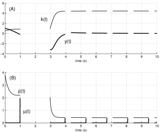
Figure 1: In graph (A), output $y(t)$ (thick line) and gain $k(t)$ are plotted. In graph (B), $\mu(t)$ (thick line) is kept at 90% of $\bar{\mu}(t)$ during blocking. A block occurs after every 1 second of continuous control.

The example of the previous paragraph is closely modeled using the variable $\mathbb{P}[a,b]$ time scale, which is continuous for an interval $a$, then has a gap for an interval $b$, then repeats. Figure 1 shows the regulation of a system implementing an adaptive gain controller in a blocking situation:

$$A=\begin{bmatrix}0&1\\ -1&1\end{bmatrix},\qquad B=\begin{bmatrix}1\\ 1\end{bmatrix},\qquad C=[1,0].$$ (23)

The gain begins at $k_{0}=\frac{1}{2}$ and the sampling period at $\mu(0)=0$. The bounding function for the graininess is $\bar{\mu}(t)=\frac{1.9}{k(t)}$ (so that $\bar{\mu}kCB<2$).

7 Conclusions

In summary, the paper illustrates a new unified continuous/discrete approach to the high-gain adaptive controller. Using recent developments in the new field of time scale theory, the unified results reveal that this type of feedback control works well on a much wider variety of time scales than explored in previous literature, including those that switch between continuous (or nearly continuous) and discrete domains or those without monotonically decreasing graininess. Furthermore, several results relating to Lyapunov analysis on time scales appear here for the first time, including Lemma 4.3 (and its use in the proof of Theorem 5.1) and 5.2. A simulation of an adaptive controller on a mixed continuous/discrete time scale is also given. It is our hope that time scale theory may find wider application in the broad fields of signals and systems as it seems that many of the tools needed in those fields are beginning to appear in their generalized forms.

We thank our colleague, Robert J. Marks II, for his very helpful suggestions throughout this project.

8 Appendix

We comment on the properties of the “expc” function referenced in the main body of the paper.

Lemma 8.1.

The power series (7) has the following properties:

1. $\operatorname{expc}(X)X=X\operatorname{expc}(X).$

2. $\operatorname{expc}(X)=(e^{X}-I)X^{-1}$ when $X^{-1}$ exists.

3. For real, scalar arguments $x$, $\operatorname{expc}(x)=e^{i\frac{x}{2}}\operatorname{sinc}(\frac{x}{2})$, where sinc denotes the sine cardinal function. (This is the motivation for the expc notation.)

4. $||\operatorname{expc}(X)||\leq\exp(||X||)$.

5. $||\operatorname{expc}(X)-I||\leq\exp(||X||)-1$.

Proof.

Parts 1-3 follow immediately from the definition. To verify 4, note

$$\left\|\sum_{n=1}^{\infty}\frac{X^{n-1}}{n!}\right\|\leq\sum_{n=1}^{\infty}\frac{||X||^{n-1}}{n!}\leq\sum_{n=1}^{\infty}\frac{||X||^{n-1}}{(n-1)!}=\exp(||X||).$$

Part 5 follows from a similar argument. Note that, by property 5, the decomposition $\operatorname{expc}(\mu X)=I+\Sigma(\mu)$ gives $||\Sigma(\mu)||\rightarrow 0$ as $\mu\rightarrow 0$, with uniform convergence. ∎

References

• [1] R. Agarwal, M. Bohner, D. O’Regan, A. Peterson, Dynamic equations on time scales: a survey, J. Computational and Applied Mathematics 141, 2002, pp 1-26
• [2] M. Bohner, A. Peterson, Advances in Dynamic Equations on Time Scales, Birkhäuser, Boston, 2003
• [3] M. Bohner, A. Peterson, Dynamic Equations on Time Scales, Birkhäuser, Boston, 2001
• [4] A. Cervin, D. Henriksson, et. al., How does control timing affect performance? Analysis and simulation of timing using Jitterbug and TrueTime, IEEE Control Systems Mag., June 2003, pp 16-30
• [5] J.J. DaCunha, Stability for time varying linear dynamic systems on time scales, J. Computational and Applied Mathematics 176 (2), 2005, pp. 381-410
• [6] J.J. DaCunha, Lyapunov Stability and Floquet Theory for Nonautonomous Linear Dynamic Systems on Time Scales, Ph.D. dissertation, Baylor University, 2004
• [7] T. Gard, J. Hoffacker, Asymptotic behavior of natural growth on time scales, Dynamic Systems and Applications 12, 2002, pp 131-147
• [8] I.A. Gravagne, J.M. Davis, J.J. Dacunha, R.J. Marks II, Bandwidth reduction for controller area networks using adaptive sampling, Proc. IEEE Int. Conf. Robotics and Automation, New Orleans, LA, April 2004, pp 5250-5255
• [9] S. Hilger, Analysis on measure chains – a unified approach to continuous and discrete calculus, Results in Mathematics 18, 1990, pp 18-56
• [10] S. Hilger, Ein Masskettenkalkul mit Anwendung auf Zentrumsmannigfaltigkeiten, Ph.D. dissertation, Universitat Wurzburg, 1988
• [11] A. Ilchmann, D.H. Owens, D. Pratzel-Wolters, High-gain robust adaptive controllers for multivariable systems, Systems & Control Letters 8, 1987, pp 397-404
• [12] A. Ilchmann, S. Townley, Adaptive high-gain $\lambda$-tracking with variable sample rate, Systems and Control Letters 36, 1999, pp 285-293
• [13] A. Ilchmann, S. Townley, Adaptive sampling control of high-gain stabilizable systems, IEEE Trans. Automatic Control 44, 1999, pp 1961-1966
• [14] A. Ilchmann, E.P. Ryan, On gain adaptation in adaptive control, IEEE Trans. Automatic Control 48, 2003, pp 895-899
• [15] H.K. Khalil, A. Saberi, Adaptive stabilization of a class of nonlinear systems using high-gain feedback, IEEE Trans. Automatic Control 43, 1987, pp 1031-1035
• [16] H. Logemann, B. Martensson, Adaptive stabilization of infinite-dimensional systems, IEEE Trans. Automatic Control 37, 1992, pp 1869-1833
• [17] D.H. Owens, Adaptive stabilization using a variable sampling rate, Int. J. Control 63, 1996, pp 107-119
• [18] D.H. Owens, D. Pratzel-Wolters, A. Ilchmann, Positive-real structure and high-gain adaptive stabilization, IMA J. Mathematical Control and Information 4, 1987, pp 167-181
• [19] N. Ozdemir, S. Townley, Integral control by variable sampling based on steady-state data, Automatica 39, 2003, pp 135-140
• [20] C. Pötzsche, S. Siegmund, F. Wirth, A spectral characterization of exponential stability for linear time-invariant systems on time scales, Discrete and Continuous Dynamical Systems 9, 2003, pp 1223-1241
• [21] J.E. Slotine, W. Li, Applied Nonlinear Control, Prentice Hall, Upper Saddle River, 1991
• [22] V. Spedding, Taming nature’s numbers, New Scientist, July 2003, pp 28-31
• [23] J.C. Willems, C.I. Byrnes, Global adaptive stabilization in the absence of information on the sign of the high frequency gain, Lecture Notes in Control and Information Sciences 62, 1984, Springer, Berlin, pp 49-57