The Building the Bridge Survey for $z=3$ Ly$\alpha$ emitting galaxies. II. Completion of the survey

Abstract

Context. We have substantial information about kinematics and abundances of galaxies at $z\approx 3$ studied in absorption against the light of background QSOs. At the same time we have studied 1000s of galaxies detected in emission mainly through the Lyman-break selection technique. However, we know very little about how to make the connection between the two data sets.

Aims. We aim at bridging the gap between absorption selected and emission selected galaxies at $z\approx 3$ by probing the faint end of the luminosity function of star-forming galaxies at $z\approx 3$.

Methods. Narrow-band surveys for Lyman-$\alpha$ (Ly$\alpha$) emitters have proven to be an efficient probe of faint, star-forming galaxies in the high redshift universe. We have performed narrow-band imaging in three fields with intervening QSO absorbers (a damped Ly$\alpha$ absorber and two Lyman-limit systems) using the VLT. We target Ly$\alpha$ at redshifts 2.85, 3.15 and 3.20.

Results. We find a consistent surface density of about 10 Ly$\alpha$-emitters per square arcmin per unit redshift in all three fields down to our detection limit of about $3\times 10^{41}\rm{ergs\;s^{-1}}$. The luminosity function is consistent with what has been found by other surveys at similar redshifts. About 85% of the sources are fainter than the canonical limit of $R=25.5$ for most Lyman-break galaxy surveys. In none of the three fields do we detect the emission counterparts of the QSO absorbers. In particular we do not detect the counterpart of the $z=2.85$ damped Ly$\alpha$ absorber towards Q2138$-$4427. This implies that the DLA galaxy is either not a Ly$\alpha$ emitter or fainter than our flux limit.

Conclusions. Narrow-band surveys for Ly$\alpha$ emitters are excellent to probe the faint end of the luminosity function at $z\approx 3$. There is a very high surface density of this class of objects. Yet, we only detect galaxies with Ly$\alpha$ in emission and hence the density of galaxies with similar broad band magnitudes will be substantially higher. This is consistent with a very steep slope of the faint end of the luminosity function as has been inferred by other studies. This faint population of galaxies is playing a central role in the early Universe. There is evidence that this population is dominating the intergrated star-formation activity, responsible for the bulk of the ionizing photons at $z\gtrsim 3$ and likely also responsible for the bulk of the enrichment of the intergalactic medium.

1 Introduction

Strong arguments (Fynbo et al., 1999; Haehnelt et al., 2000; Schaye, 2001; Rauch et al., 2008; Barnes & Haehnelt, 2008) indicate that there is very little overlap between emission selected galaxies (primarily Lyman-Break Galaxies, LBGs, Steidel et al., 2003) and absorption selected galaxies (primarily the Damped Lyman-$\alpha$ Absorbers, DLAs Wolfe et al., 2005). The simple reason for this is that LBG samples are continuum flux limited and that the current flux limit of R$\approx$25.5 is not deep enough to reach the level of typical absorption selected galaxies. This is unfortunate as we then know little about how to combine the detailed information on abundances and kinematics inferred from observations of DLAs with the information about colours and luminosities of high-$z$ galaxies detected in emission.

In 2000 we started a survey aiming at bridging the gap between emission and absorption selected galaxies. The goal of the survey was to detect faint $z\approx 3$ galaxies using narrow-band imaging selection of Lyman-$\alpha$ (Ly$\alpha$) emitters (LAEs) and in this way bridge the gap between the DLAs and the LBGs. During the 1990ies and early 2000s it was established that LAEs can be used to select high-z galaxies (e.g. Møller & Warren, 1993) and that this method easily traces significantly deeper into the luminosity function than what is possible with spectroscopic samples of LBGs (e.g. Cowie & Hu, 1998; Fynbo et al., 2001). In our survey we targeted the fields of QSOs with intervening DLAs primarily to be able also to search for the galaxy counterparts of the DLAs, but also to anchor the fields to known structures at the targeted redshifts. The first paper of the survey was published by Fynbo et al. (2003) (hereafter Paper I), where we presented the results from two of the three targeted fields. Since then the study of LAEs has progressed substantially, mainly on two fronts. First, large samples covering a range of redshifts have been collected using wide-field imagers both on 4m and 8m class telescopes (e.g. Gronwall et al., 2007; Ouchi et al., 2008; Nilsson et al., 2008). Second, more detailed studies of the properties have been carried through, most notably based on LAEs in the GOODS fields (e.g. Nilsson et al., 2007; Gronwall et al., 2007; Pentericci et al., 2008).

In this final paper from our ”Building the bridge” survey we first present the results from the third field, namely the sample of LAEs identified in the field of the quasar BRI 1202$-$0725. Second, we combine the results of the entire survey covering three fields to derive the luminosity function of the LAEs at $z\sim 3$. We then discuss our results in the light of the substantial progress that has been made by a number of groups over the last few years on the study of LAEs at $z\gtrsim 2$.

Throughout this paper, we assume a cosmology with $H_{0}=70$ km s^-1 Mpc^-1, $\Omega_{\rm m}=0.3$ and $\Omega_{\Lambda}=0.7$. We also throughout use magnitudes on the AB system (Oke, 1974).

2 The field of BRI 1202$-$0725

2.1 Imaging

The field of BRI 1202$-$0725 ($z_{\rm qso}=4.70$) was included in this survey due to the presence of a Lyman-limit system along the line-of-sight towards the quasar at a redshift of $z=3.2$ (Storrie-Lombardi et al., 1996). This field was observed in service mode at the VLT 8.2 m telescope, unit Yepun, during the nights January 30 through February 6 2003 using the FORS2 instrument. The wavelength of the Ly$\alpha$ transition at the redshift of $z=3.20$ is $\lambda=5105{\AA}$, which corresponds to the central wavelength of the 61Å wide [OIII] VLT filter. The field was observed in this narrow-band filter (NB) and in the Bessel $V$ and Special $R$ filters. The transmission curves of the three filters are shown in Fig. 1. The integration times in the $V$ and $R$ filters were set by the criterion that the broad on-band $V$ imaging should reach about half a magnitude deeper than the narrow-band imaging so as to get a reliable selection of objects with excess emission in the narrow-band filter. For the broad off-band $R$ imaging, we aimed at reaching the $5\sigma$ significance level at one magnitude deeper than the spectroscopic limit of $R$(AB)=25.5 for LBGs (i.e. aiming at $R$(AB)=26.5 at the $5\sigma$ significance level). The total integration times, the seeing (FWHM) of the combined images and the 5$\sigma$ detection limits for a 3″diameter aperture are given for each filter in Table 1. For comparison with previous work we also list the corresponding numbers for the fields of BRI 1346$-$0322 and Q 2138$-$4427 presented in Paper I.

Figure 1: Transmission curves of the narrow- and broad-band filters used for the observations of BRI 1202$-$0725.

Table 1: Log of imaging observations with FORS1 and 2 of the three surveyed fields. The $5\sigma$ detection limits are computed for a 3″diameter aperture. The data for BRI 1346$-$0322 and Q 2138$-$4427 are reproduced from Paper I.

filter	$z_{\rm qso}$, $z_{\rm abs}$	total exp.	PSF fwhm	5$\sigma$
		time (hr)	($\arcsec$)	limit
BRI 1202$-$0725	4.70, 3.20
$N$		8.3	1.02	25.6
$V$		2.9	0.96	26.6
$R$		1.6	0.95	26.1
BRI 1346$-$0322	3.99, 3.15
$N$		8.9	0.93	25.6
$B$		2.5	1.02	26.6
$R$		1.7	0.94	26.0
Q 2138$-$4427	3.17, 2.85
$N$		10.0	0.96	26.5
$B$		2.5	1.04	26.9
$R$		1.7	0.93	26.3

The images were reduced (de-biased and corrected for CCD pixel-to-pixel variations) using the FORS pipeline (Grosbøl et al., 1999). The individual reduced images in each filter were combined using a code that optimizes the Signal-to-Noise (S/N) ratio for faint, sky-dominated sources (see Møller & Warren 1993 for details on this code).

The broad-band images were calibrated as part of the FORS calibration plan via observations of Landolt standard stars (Landolt 1992). We transformed the zero-points to the AB system using the relations given by Fukugita et al. (1995): $V$(AB)=$V$$-0.02$ and $R$(AB)=$R$$+0.17$. For the calibration of the narrow-band images, we used observations of the spectrophotometric standard stars EG274 and GD71.

2.2 LAE candidate selection

The selection of LAE candidates is based on the “narrow minus on-band broad” versus “narrow minus off-band broad” colour/colour plot technique (Møller & Warren, 1993; Fynbo et al., 1999, 2000, 2002, 2003). The object identification and photometry was carried out in SExtractor (Bertin & Arnouts, 1996) using the dual-image mode having a detection image and measuring the photometric properties on the individual images. For the detection we used a weighted sum of the $V$-band (20%) and narrow-band (80%) images to secure an optimal detection of objects with excess in the narrow filter. Before object detection we convolved the detection image with a Gaussian filter function having a FWHM equal to that of point sources. We used a detection threshold of 1.1 times the background sky-noise and a minimum area of 5 connected pixels in the filtered image. For total magnitudes we use the SExtractor MAG_AUTO and to compute colours we use the isophotal magnitudes (MAG_ISO). In our final catalogue, we include only objects with total S/N$>$5 in the isophotal aperture in either the narrow- or the $V$-band images. In total, we detect 3202 such objects within the 400$\times$400 arcsec² field around BRI 1202$-$0725. The error bars on the colour indices are derived using the maximum likelihood method of Fynbo et al. (2002). For the selection of LAE candidates we restricted the sample to S/N$>$5 in the narrow-band filter as described below.

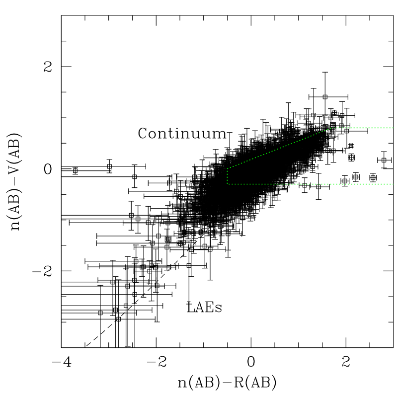
Figure 2: Left panel: Colour-colour diagram for simulated galaxies based on Bruzual & Charlot 1995 galaxy SEDs (Bruzual & Charlot, 2003). The open squares are 0$<$z$<$1.5 galaxies with ages ranging from a few to 15 Gyr and the open triangles are 1.5$<$z$<$3.0 galaxies with ages ranging from a few Myr to 1Gyr. The dotted box encloses the simulated galaxy colours. The dashed line indicates colours of objects with a particular broad-band colour and with an SED in the narrow-band filter ranging from an absorption line in the upper right part to a strong emission line in the lower left part of the diagram. Middle panel: Colour-colour diagrams for all objects detected at S/N$>$5 in either the narrow band or the $V$ band in the BRI 1202$-$0725. In the lower left part of the diagram there is a large number of objects with excess emission in the narrow filter. Candidate LAEs are those objects with a 1$\sigma$ upper limit on $N$(AB)$-V$(AB) below the 98% percentile. Right panel: The colours of the QSOs and of the LAE candidates are indicated. Candidates confirmed to be emission line objects based on our spectroscopic observations described in Sect. 2.3 are shown by filled symbols. Candidates that cannot be confirmed by the present spectroscopy are indicated by open symbols. The solid line indicates the median $N(\rm{AB})-V(\rm{AB})$ colour for all detected objects as a function of $N(\rm{AB})-R(\rm{AB})$ and the dotted lines indicate the 2% and 98% percentiles in the $N(\rm{AB})-V(\rm{AB})$ colour. The horisontal dotted line denote our selection of $N(\rm{AB})-V(\rm{AB})<-1$.

In Fig. 2 we show the colour-colour diagram used for the final selection of LAE candidates. In order to constrain where objects with no special spectral features in the narrow filter are in the diagram, we calculated colours based on synthetic galaxy SEDs taken from the Bruzual & Charlot 1995 models (Bruzual & Charlot, 2003). We have used simple single-burst models with ages ranging from a few Myr to 15 Gyr and with redshifts from 0 to 1.5 (open squares in Fig. 2) and models with ages ranging from a few Myr to 1 Gyr with redshifts from 1.5 to 3.0 (open triangles). For the colours of high-redshift galaxies, we included the effect of Ly$\alpha$ blanketing (Møller & Jakobsen, 1990; Madau, 1995), but for none of the models the effects of dust are included. Fig. 2 shows the N(AB)$-V$(AB) versus N(AB)$-$$R$(AB) colour diagram for the simulated galaxy colours (left panel) and for the observed sources in the target field (middle and right panels). The dashed line indicates where objects with a particular broad-band colour (corresponding to a 100 Myr old galaxy at $z=3.20$ and either absorption (upper right) or emission (lower left) in the narrow filter will fall.

In the middle panel, we show the colour-colour diagram for all of the objects detected in the field. The large, dense group of points correspond to the normal field galaxy population without special properties in the narrow-band filter, in the following refered to as continuum objects. Unfortunately, the observed distribution of the continuum objects is oriented along the same direction as that expected for emission line objects (indicated with the dashed line). This is due to the fact that the central wavelength of the narrow-band filter is bluewards of the central wavelength of the on-band broad filter ($V$). For this reason we for this field choose a rather conservative criterion for selection of candidates, namely $N(\rm{AB})-V(\rm{AB})<-1$. After weeding out a few spurious sources (related to bright stars) we detect 25 such objects in the BRI 1202$-$0725 field which we consider as LAE candidates in the following. The colours of the candidates are shown in the right panel of the figure.

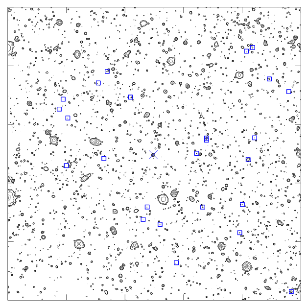
Figure 3: The 400$\times$400 arcsec² field surrounding the QSO BRI 1202$-$0725 as observed in the narrow-band filter. North is up and East is to the left. The QSO is identified by a “$\times$” at the field centre and the positions of candidate LAEs are shown with boxes.

A contour image of the combined narrow-band image of the 400$\times$400 arcsec² field surrounding the QSO BRI 1202$-$0725 is shown in Fig. 3. The QSO is identified by a “$\times$” at the field centre and the positions of selected LAE candidates are shown with boxes.

Figure 4: Our equivalent width selection criterion is illustrated by plotting the line equivalent width against the Ly$\alpha$ flux in the isophotal aperture for the LAE candidates. The continuous line shows our N(AB)$-$$V$(AB) colour selection criterion converted into equivalent width. Filled symbols indicate objects subsequently confirmed by spectroscopy to be emission-line sources. Open circles indicate objects that were observed, but not confirmed. The error bars on EWs are derived as described in Fynbo et al. (2002).

In the selection of LAE candidates we apply a colour selection which translates into the equivalent width (EW) selection criterion illustrated in Fig. 4 given in observed quantities. The selection criterion translates into candidates having observed EW$\gtrsim 100$Å (or rest frame EW$\gtrsim 25$Å).

2.3 Multi-object spectroscopy

The above selection of LAE candidates only selects for excess emission in the narrow-band filter. This is likely to originate from the Ly$\alpha$ at $z\sim 3.2$ (Fynbo et al., 2003), however, interlopers caused by other emission lines in galaxies at lower redshifts is also possible. Therefore, follow-up spectroscopy is necessary for confirming the Ly$\alpha$ origin of the excess emission.

Follow-up multi-object spectroscopy (MOS) was carried out in visitor mode on March 21–23, 2004, with FORS2 installed at the VLT telescope, unit Yepun. The mask preparation was done using the FORS Instrumental Mask Simulator. The field of BRI 1202$-$0725 was covered by 3 masks. It was possible to fit all candidates into the slits. The spectra were obtained with the G600B grism covering the wavelength range from 3600Å to 6000Å at a resolving power of 900. For possible identification of other emission lines at the same redshift we also obtained spectra with the G600R grism covering the wavelength range from 5000Å to 7500Å. The detector pixels were binned 2$\times$2 for all observations through the masks. In Table LABEL:tab:spec-journal we give the main characteristics of the spectroscopic observations.

Table 2: Log of spectroscopic observations with FORS2.

mask	Exp.time	Date	Effective seeing
	(hr)	(2004)	($\arcsec$)
mask1202A	6.3	March 21-23	0.94
mask1202B	6.0	March 21-23	0.76
mask1202C	5.0	March 21-23	0.96

The MOS data were reduced and combined as described in Fynbo et al. (2001). The accuracy in the wavelength calibration is about $\pm$0.1 pixel for a spectral resolution of $R=900$, which translates to $\Delta z=0.0002$. Average object extraction was performed within a variable window size matching the spatial extension of the emission line. Therefore, the flux should be conserved.

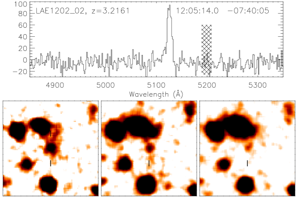
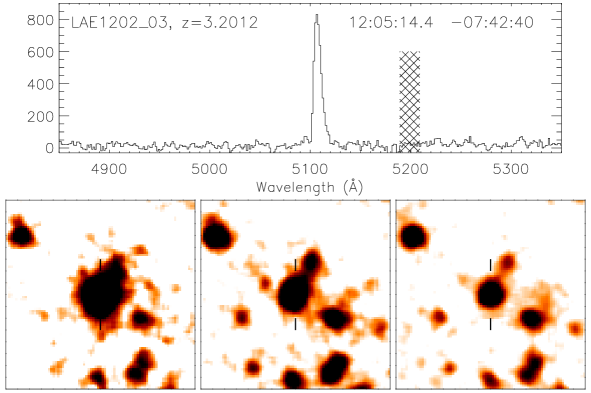
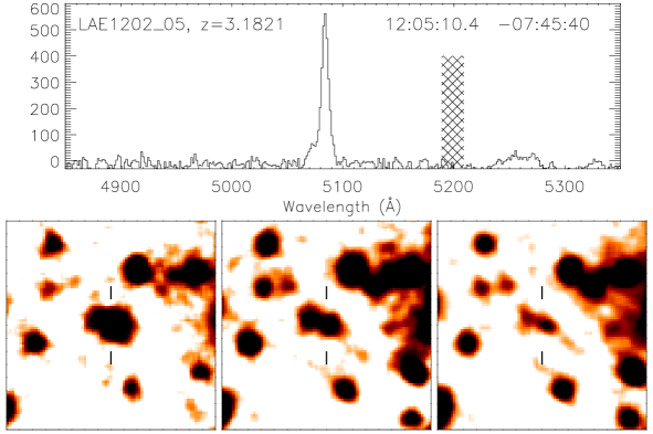
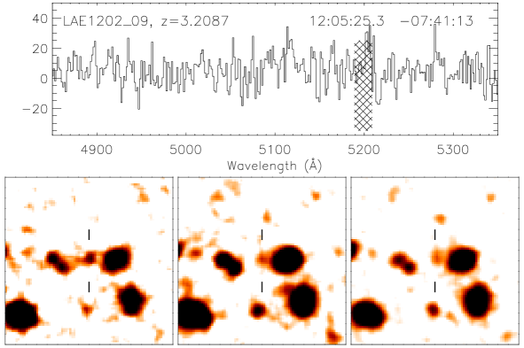
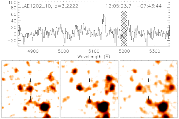
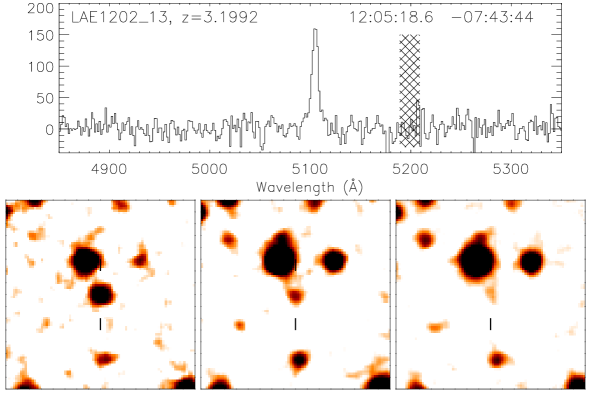
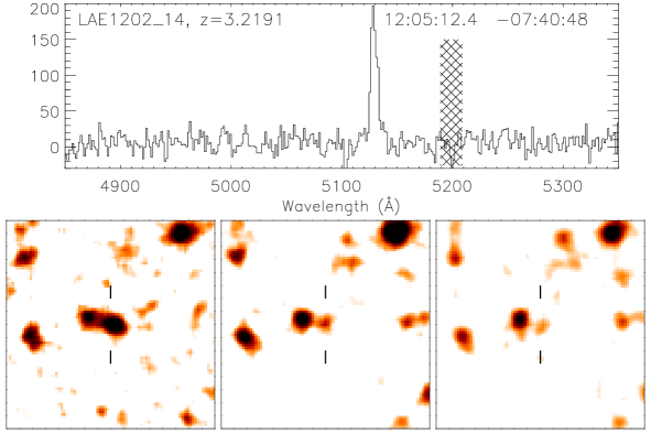
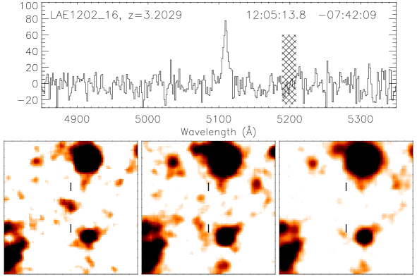
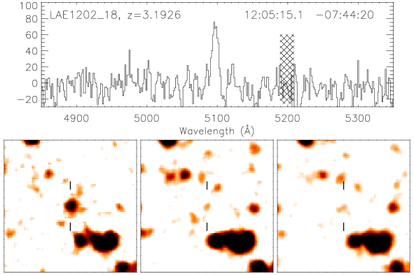
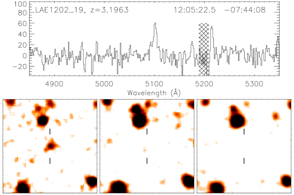
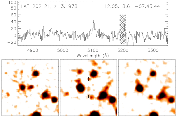
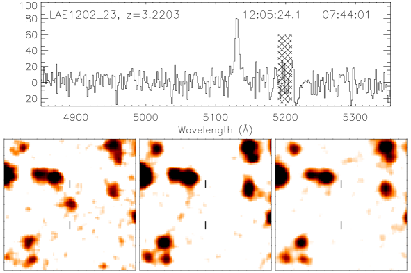
Figure 5: 16$\times$16 arcsec² images and 1-D spectra of 18 (note that candidates # 8 and 11 are covered by the same spectrum) confirmed LAEs in the field of BRI 1202$-$0725. The hatched areas have been excluded from the analysis due to the overlap with night-sky lines. The units on the ordinate of the spectra are counts in 1800 sec. The name, redshift and coordinates (Epoch 2000) are provided for each object. For each candidate, we show images from the $N$-, $V$- and $R$-band filters (from left to right) with North up and East to the left.

Of the 25 targeted LAE candidates, 18 are confirmed emission line objects. For the seven remaning candidates no emission line was identified in the spectrum. The spectra for the 18 confirmed candidates are shown in Fig. 5. We consider a candidate confirmed if there is an emission line detected with at least $3\sigma$ significance at the correct position in the slitlet within the wavelength range corresponding to the filter transmission. All of the confirmed emission line candidates are most likely to be Ly$\alpha$ based on the absence of other emission lines at longer wavelengths (mainly NeIII , H$\beta$ and O[III] , the positions of which are all covered by our spectroscopy). The limits on the flux ratios we infer are similar to those derived in Fynbo et al. (2001) and based on their analysis contamination from OII emitters is very unlikely. The overall efficiency for detection and confirmation of LAEs is therefore #(confirmed LAEs)/#(observed LAEs)=18/25=72%. This is the same as found for Q 2138$-$4427 and somewhat less than the results of BRI 1346$-$0322 (Paper I).

The redshift distribution for the LAE sample in the field of BRI 1202$-$0725 is shown in Fig. 6 and compared with the filtercurve. It can be seen that the targets fill out the volume probed by the filter. The mean redshift of the LAEs is 3.203 with a standard deviation of 0.013.

Figure 6: Redshift distribution of LAEs in the field of BRI 1202$-$0725 relative to the filter transmission curve. The redshifts of LAEs fill out the volume probed by the filter.

We have investigated the properties of the non-confirmed candidates and find that they are in the red end of the broad-band colours of the candidate sample and unresolved. However, their low line fluxes prevent them from being confirmed by the present spectroscopic observations. This analysis was carried out for all three fields and we found similar properties in all cases.

3 The LAE population

In the following we combine the results of the entire Building the Bridge Survey to characterise the population of LAEs. The survey constitutes observations of three fields centered on the quasars BRI 1202–0725, BRI 1346–0322 and Q 2138–4427 searching for Ly$\alpha$ emitters at redshifts $z=3.20,3.15$ and 2.85, respectively. These redshifts are targeted due the presence of high column density absorption systems along the line of sight towards the quasars. In the fields 25, 26 and 36 emission line objects were identified through the narrow-band technique. In each of the fields of BRI 1346–0322 and Q 2138–4427 the emission from two emitters were identified with other emission lines than Ly$\alpha$ (in three cases corresponding to [OII]  and the fourth case CIV , Fynbo et al., 2003). Therefore, these four objects have been excluded from the current analysis. In the following analysis we consider 18, 18 and 23 spectroscopically confirmed LAEs as the confirmed sample. The entire photometric sample includes 7, 6 and 11 additional objects. These have not been confirmed spectroscopically. For the fields of BRI 1202–0725 and Q 2138–4427 all candidates were observed, so the non-confirmed systems were lacking an emission line at our sensitivity. For the field BRI 1346–0322 three candidates were not observed leaving three as spectroscopically not confirmed candidates.

Table 3: Overview of LAE samples from the three fields included in the present survey.

Field	z	$N_{tot}$	$N_{conf}$	$N_{non}$	Dens.(conf)	EW0,conf	EW0,non	$L_{conf}$(Ly$\alpha$)	$L_{non}$(Ly$\alpha$)d	SFRconf	SFRnon
					$arcmin^{-2}\Delta z^{-1}$	Å	Å	1041 erg s-1	1041 erg s-1	M⊙yr-1	M⊙ yr-1
BRI 1202–0275	3.20	25	18	7	8	$\geq 27$	$\geq 21$	$\geq 6.06$	$\geq 4.07$	$\geq 0.62$	$\geq 0.42$
BRI 1346–0322	3.15	24	18	6	8	$\geq 22$	$\geq 26$	$\geq 12.21$	$\geq 9.92$	$\geq 1.25$	$\geq 1.02$
Q 2138–4427	2.85	34	23	11	10	$\geq 20$	$\geq 18$	$\geq 3.66$	$\geq 4.58$	$\geq 0.38$	$\geq 0.47$

The LAE population is characterised in terms of magnitudes, colours and derived entities like Ly$\alpha$ flux, luminosity, EWs and star formation rates (SFRs). For total magnitudes we use the SExtractor MAG_AUTO which are used to compute the Ly$\alpha$ flux, luminosity and SFR. The colour indices are computed based on isophotal magnitudes (MAG_ISO) and are used to estimate the EW. For all magnitudes the same detection area is used in all bands. Details of the computation of the derived properties can be found in Fynbo et al. (2002). Finally, in the next section we derive the luminosity function of LAEs at $z\sim 3$ and compare this with the recent measurements by Gronwall et al. (2007); Ouchi et al. (2008) and Rauch et al. (2008). Table 3 gives an overview of the LAE samples of the three fields. From the table it can be seen that the survey covers LAEs with luminosities in Ly$\alpha$ down to a few times $10^{41}$ ergs  s^-1, making it one of the deepest surveys of Ly$\alpha$ emitters at z$\approx 3$. Table 4 summarises the main characteristics of our sample and the three used for comparison.

Table 4: Summary of the main properties of our and the comparison samples.

Ref.	Type	z	N	Area	Ly$\alpha$ luminosity
				sq.arcmin	ergs  s-1
This sample	Spectroscopic/photometric	$\sim$3.0	59/83	133	$\gtrsim$0.3$\cdot$1042
	Around absorption systems
Serendipitous	Spectroscopic	$2.30\leq z\leq 3.61$	6	$-$	$-$
	Field
Gronwall et al. (2007)	Photometric only	$\sim$3.1	162	1008	$\gtrsim 1.3\cdot$1042
	Field
Ouchi et al. (2008)	Photometric only	$\sim 3.1$	356	3538	$\gtrsim 10^{42}$
	Field
Rauch et al. (2008)	Long-slit spectroscopy	$2.67\leq z\leq 3.75$	27	$-$	$(0.015-1.73)\cdot 10^{42}$
	Field

3.1 Characteristics of spectroscopically confirmed LAEs

Figure 7: Total magnitude (MAG_AUTO) distribution of the LAEs in Narrow- (top) and $R$-band (bottom). The curves are averages between fields and error bars are the corresponding standard deviations. Open circles and dotted lines mark the distribution for all photometrically selected candidates, while filled symbols and solid lines mark the confirmed Ly$\alpha$ emitters. The triangles indicate $1\sigma$ upper limits for galaxies detected at lower levels. The arrow in the lower plot marks the $R=25.5$ limit for spectroscopic surveys of absorption line systems. It should be noted that for the candidate selection the isophotal magnitudes were used and here we use total magnitudes. All magnitudes have been rescaled to $z=3$, though neglecting the small differences in k-correction for the $R$-band.

In Tables 7–9 we give the measured and derived properties for the confirmed LAEs. The magnitudes in these tables are total magnitudes, and the lower limits correspond to $1\sigma$ significance levels for the SExtractor MAG_AUTO apertures. These translate into the limits given for the fluxes and luminosities. The EWs are derived from the colour indices based on the isophotal magnitudes. In this case the limits are caused by a less significant detection in the on-band broad ($B$ or $V$) and the values correspond to using the $1\sigma$ levels for these bands.

From Table 3 it can immediately be seen that the total number of objects is comparable among the three fields. The detected number of LAEs translates into surface densities of 8, 8 and 10 per square arcmin per unit redshift, respectively for the fields of BRI 1202–0275, BRI 1346–0322 and Q 2138–4427, consistent with the almost similar flux limits in the three fields. From the table it can also be seen that the other properties are similar between the fields and between the confirmed LAEs and non-confirmed candidates.

In Fig. 7 we show the magnitude distribution for the LAEs. The lines correspond to candidates with measured magnitudes while the triangles indicate systems with $1\sigma$ upper limits. The observed magnitudes are translated to correspond to a redshift $z=3$ by correcting by the difference in the distance modulus between the observed redshift and $z=3$. For the $R$-band we do not apply any K-correction since it is a negligible effect over such small redshift changes. The errorbars are standard deviations among the fields and indicate that even though the results in the three fields are consistent, small numbers and cosmic variance leads to significant differences between the fields. For the narrow-band it is clear that all the bright objects have been confirmed to correspond to Ly$\alpha$ emitters while the non-confirmed cases are in general found in the faint end of the distribution.

From the magnitude distribution of the $R$-band it can be seen that all the LAE candidates have very faint magnitudes. For absorption line systems the magnitude limit of achieving a redshift is $R$$\sim$25.5 indicated by the arrow in the figure. Therefore, we note that of the confirmed emitters only 6 out of 59 or $\lesssim$10% are brighter than this limit. The fraction is similar for the complete candidate sample. This is consistent with the non-confirmed candidates being spread over all $R$-band magnitudes. The faint $R$-band magnitudes of the galaxies emphasises their importance for tracing the faint end of the luminosity function, possibly contributing a significant fraction of the total star formation (see also Reddy & Steidel, 2008).

Figure 8: Rest frame equivalent width distribution for the confirmed (solid symbols and line) and entire (open symbols and dashed line) samples (upper panel). In the lower panel the distribution for the confirmed sample is compared with that of (Gronwall et al., 2007, dot-dashed line) and (Ouchi et al., 2008, dashed line). The triangles indicate cases for which only lower limits (at the $1\sigma$ level) could be determined.

Fig. 8 shows the distribution of rest frame equivalent widths derived from the colour index “narrow band minus on-band broad” isophotal magnitudes. We have not corrected the broad-band magnitudes for the narrow-band contribution. Our measurements are compared with those of Gronwall et al. (2007) and Ouchi et al. (2008). It can be seen that the sample of confirmed LAEs for which we could measure the EW reliably is consistent with our survey being deeper than the comparison samples. It can also be seen that the Ouchi et al. sample has a higher fraction of emitters with high EW than the Gronwall et al sample. Our sample it is more consistent with the Ouchi et al. than with the Gronwall et al. sample.

Table 3 also lists the range of SFR derived from the Ly$\alpha$ luminosities (following Fynbo et al. 2002). The SFRs are found to be in the range $0.38M_{\odot}$yr^-1 to $31M_{\odot}$yr^-1 assuming negligible extinction.

4 Luminosity function of LAEs at $z\sim 3$

A widely used diagnostic for describing galaxy samples is their luminosity function (LF). Here, we derive the LF of LAEs at $z=3.0$ combining the data from the present work and from Paper I. The complete survey encompasses three fields with a total of 59 spectroscopically confirmed LAEs. For each field we derive the LF independently to take into account the different narrow-band filters and incompleteness functions. Finally, the individual results are combined to provide the LF at $z=3.0$.

4.1 Estimating the incompleteness correction

Figure 9: Completeness levels as function of Ly$\alpha$ luminosity. The dotted line corresponds to the field of BRI 1202–0725; dashed line to BRI 1346–0322 and triple dot-dashed line to Q 2138–4427.

When constructing the sample of LAEs the main source of incompleteness comes from the photometric selection of candidates. The following process is carried out separately for each field to take into account the specific properties of the different data sets. To estimate the detection completeness of the photometric samples we distribute 100 artificial objects in the images and assign broad- and narrow-band magnitudes in a range covering the observed values as well as an additional margin. The magnitudes were assigned based on the off-broad band. In this band magnitudes are distributed uniformly in the interval 5 to 35. For the narrow- and on-broad bands magnitudes were assigned based on a uniform colour index (“narrow $-$ off-broad” and “on-broad $-$ off-broad”) distribution in the interval minus five to five. This results in uniform magnitude distributions in the narrow- and on-broad bands in the magnitude interval 10 to 30 dropping off and vanishing at magnitudes of zero and 40. The objects are modeled with a two-dimensional gaussian shape with the size corresponding to the seeing measured in the individual images. Each artificial object is added to each image scaling the gaussian to the appropriate luminosity depending on the magnitudes computed individually for each band. This process ensures good coverage for both magnitudes and colour indices. The procedure is repeated 1000 times for each field, thus a total of 10⁵ artificial objects are used in the estimate. The images with artificial objects are now treated exactly as the original images and the recovery rate yields the detection completeness. The completeness functions estimated for the three fields in the narrow-band filters are shown in Fig. 9. From that figure it can be seen that the data of the field of BRI 1346–0322 are slightly shallower than the other two fields, which are very similar. These completeness functions are used to correct the measured luminosity functions below. Note that we have not corrected our data for the effects of a non-square band-pass or the photometric error function (see Gronwall et al., 2007).

A possible concern is whether the extension of the Ly$\alpha$ emitters have a significant effect on the estimated completeness functions. To test this we have carried out a complementing test where the original background subtracted images were first dimmed. Then we corrected the background noise to the original level and tried to recover the already detected candidate emitters. We dimmed the images by 0.25, 0.5 and 0.75 magnitudes. The completeness functions estimated in this way were similar to the ones described above, but suffer from poor statistics (only 80 sources in total were found in the original images) and only tracing the magnitudes and colour indices of the detected sources. This makes the previously described functions more reliable for correction purposes and are the ones used in the following.

4.2 Ly$\alpha$ luminosity function

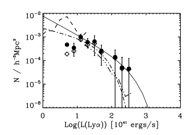
Figure 10: The derived differential Ly$\alpha$ luminosity function for the sample of confirmed (upper) and all (lower) LAEs. The points with open symbols are not corrected for incompleteness, while those with solid symbols are. The thin solid line indicate our fit to the confirmed candidates. The thick solid and dotted lines in the lower panel mark the fits to the deep and brighter sample of all cadidates, respectively. The error bars are obtained from the $1\sigma$-error bars of the individual fields by standard error propagation.

The fits are described in detail in the text. Our result is compared with the luminosity function for emitters at $z=3.1$ by Ouchi et al. (2008) in triple-dot dashed line, Gronwall et al. (2007) in dot-dashed line and Rauch et al. (2008) in dashed line.

We derive the differential luminosity function for the confirmed LAEs with a simple classical approach that has been used in many previous works (e.g. Ouchi et al., 2003; Ajiki et al., 2003; Hu et al., 2004; Malhotra & Rhoads, 2004; Ouchi et al., 2008). The volume used to convert the observed number of systems to volume densities is computed based on the field size and having a depth corresponding to the FWHM of the narrow-band filter. Furthermore, we correct the observed luminosity function by the completeness function estimated in the previous section to account for the incompleteness of the sample due to our target selection. The obtained luminosity function is shown in Fig. 10. The error-bars are derived from the errors in the individual fields by standard error propagation.

We fit our derived LF with the Schechter function (Schechter, 1976) using a $\chi^{2}$-minimisation. We carry out three fits in total. First, we fit the sample of confirmed candidates with $L^{*}>=10^{42}\mathrm{ergs\;s^{-1}}$. Second, we fit the entire photometric sample in two luminosity intervals: $L^{*}>=10^{42}\mathrm{ergs\;s^{-1}}$ and $L^{*}>=10^{41.6}\mathrm{ergs\;s^{-1}}$. The brighter limit corresponds to the region where all fields are estimated to be close to complete, while the second limit is where the shallowest field is essentially not contributing anything (see Fig. 9). The results of the fits are summarised in Table 5. In Fig. 10 we include the fit to the confirmed candidates as the thin solid line in both panels and the fit to the deep sample of all candidates is included in the lower panel as the thick solid line. The fit to all candidates with the brighter luminosity limit is included as the dotted line. It can be seen that despite the small differences in the best fit parameter values the functions are consistent.

Table 5: Results of fitting a Schechter function to the LF.

Type	$\log(L^{*})$	$\alpha$	$\phi$	$\chi^{2}$
	(ergs  s-1)		$h^{-3}Mpc^{3}$
Confirmed, $\log(L^{*})>=42$	$43.55_{-0.10}^{+0.05}$	$-1.80_{-0.06}^{+0.08}$	$1.5_{-0.3}^{+0.3}\cdot 10^{-4}$	0.32
All, $\log(L^{*})>=42$	$43.30_{-0.05}^{+0.05}$	$-1.74_{-0.04}^{+0.06}$	$3.2_{-0.5}^{+0.5}\cdot 10^{-4}$	0.28
All, $\log(L^{*})>=41.6$	$43.15_{-0.05}^{+0.05}$	$-1.58_{-0.04}^{+0.06}$	$5.8_{-0.8}^{+0.8}\cdot 10^{-4}$	2.06

We compare our result with those of Gronwall et al. (2007); Ouchi et al. (2008) and Rauch et al. (2008). At the faint end we find a good agreement, in particular if all the non-confirmed candidates are LAEs. At the bright end we find a marginal excess of objects compared to the other surveys, even though the numbers are consistent within the error bars. The (marginal) excess of bright objects may be caused by enhanced clustering of bright LBGs around QSO absorber fields (Bouché & Lowenthal, 2004; Bouché et al., 2005). Comparing the density of galaxies brighter than the limit of Gronwall et al. (2007) of $13\cdot 10^{41}\rm{ergs\;s^{-1}}$ we find only a marginal excess of a factor of $\sim 1.25$. It is also interesting to compare these environments with the results of Venemans et al. (2007) studying radio galaxies. The radio galaxies traces the largest overdensities, likely representing proto-clusters. The overdensity of LAEs around radio galaxies are found to be of the order 2-5. Thus the overdensities found in our fields are, as expected, smaller. In the field of Q 2138–4427 the redshifts are concentrated relative to the width of the filter function (Paper I, see also Monaco et al. (2005)). In this field the overdensity is only a factor of 1.1 with respect to the results of Gronwall et al. (2007), thus we do not consider this good evidence for a proto-cluster.

5 Galaxy counterparts of the QSO absorbers

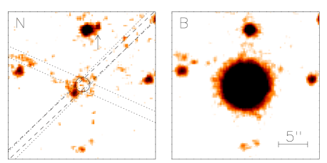
Figure 11: FORS 1 narrow-band image centered on Q 2138$-$4427 (left panel). North is up and East is to the left. The wavelength at peak transmission of the (Heii) narrow-band filter used corresponds to Ly$\alpha$ emission at $z=2.85$. The PSF of the QSO was carefully subtracted which reveals a source only $1\aas@@fstack{\prime\prime}4$ away from the QSO line-of-sight. The different orientations of the slits during the MOS observations (Paper I) and the complementary deep long-slit spectroscopic follow-up are shown by, respectively, dotted and dashed lines. The arrow in the upper part of the image marks the location of the closest LAE (LEGO2138_36) that was selected by comparing the narrow-band image with the FORS 1 $B$ and $R$ broad-band images. In the right panel, the $B-$band image is shown with the same scale and orientation as the narrow-band image.

One of the goals of our survey was to bridge the gap between emission and absorption selected objects. The three studied fields are centered on QSOs with high column density absorption systems at the redshift for which Ly$\alpha$ falls in the narrow-band filters. In the fields of BRI 1346$-$0322 and BRI 1202$-$0725 the absorbers are Lyman-limit systems and in the field of Q 2138$-$4427 it is a DLA. The observed flux of Q 2138$-$4427 is reduced by approximately 1.5 magnitude in the narrow-band image as shown in Fig. 3 of Paper I. This is due to the strong DLA line that absorbs the QSO light making it much easier to search for any faint emission close to the QSO in the narrow band than in the broad-band images. Moreover, if the galaxy counterpart of the $z_{\rm abs}=2.852$ DLA system has Ly$\alpha$ emission, it would be relatively brighter in the narrow-band than in the broad-band images. To subtract the image of the QSO in the narrow-band image, we used PSF-subtraction. We modelled the PSF of the QSO from ten bright, yet unsaturated, stars present in the field. The extension ALLSTAR of the DAOPHOT-II software (Stetson, 1987, 1994) was used to perform the final PSF model fitting and subtraction. After careful PSF subtraction, we detected an extended source at an impact parameter of $1\aas@@fstack{\prime\prime}4$ (corresponding to 12 kpc at $z=2.85$) from the QSO line-of-sight at a position angle of $136.5^{o}$ (see Fig. 11). The proximity of this source to the QSO line-of-sight makes it a good candidate for the DLA galaxy counterpart.

Figure 12: (a) portion of the 2-D long-slit spectrum of Q 2138$-$4427 centered on the Ly$\alpha$ trough of the DLA system at $z_{\rm abs}=2.852$ (first top panel). In the second top panel, the PSF of the QSO has been subtracted using the Spectral PSF II optimal extraction algorithm (Møller et al., 2000). (b) same as above for the DLA system at $z_{\rm abs}=2.383$ toward Q 2138$-$4427 (bottom two panels). The host galaxies of the DLA systems are detected in neither case. The object seen in the narrow-band image shown in Fig. 11 must be a continuum source.

To establish whether the source seen in Fig. 11 is the galaxy counterpart of the $z_{\rm abs}=2.852$ DLA system, we gathered spectra of Q 2138$-$4427 using both FORS 1 Multi-Object Spectroscopy (MOS) and long-slit spectroscopy. The details of the MOS observations were given in Paper I. The positions of the two MOS slitlets that covered the QSO are marked with dotted lines in the left panel of Fig. 11. One of the $1\aas@@fstack{\prime\prime}4$-wide MOS slitlets covered both the QSO and the candidate DLA galaxy counterpart while the second MOS slitlet was oriented at a position angle about $70\degr$ smaller. None of these spectra showed Ly$\alpha$ emission from the DLA absorber. However, the atmospheric conditions during the MOS observations were quite poor (see Paper I) and we consequently obtained a deeper ($\sim 5$ hr total integration time) FORS 1 long-slit spectrum with a $1\aas@@fstack{\prime\prime}0$-wide slit and the G600 B grism covering the candidate under very good seeing conditions (${\rm FWHM}=0\aas@@fstack{\prime\prime}71$ in the combined spectrum). The position of the long slit is shown with dashed lines in Fig. 11. The 2-D long-slit spectrum is displayed in the upper two panels of Fig. 12. We used the spectral PSF II optimal extraction algorithm (Møller et al., 2000) to subtract the emission from the QSO in the wings of the DLA trough. No Ly$\alpha$ emission from the candidate DLA galaxy counterpart is detected.

We conclude that the source seen in Fig. 11 is not an LAE at $z=2.85$. Possible Ly$\alpha$ emission from this source should be fainter than the $3\sigma$ very low detection limit of $\sim 4\times 10^{-18}$ erg s^-1 cm^-2. Within $1\arcsec$ from the QSO line-of-sight, our detection limit for Ly$\alpha$ emission is even lower (by less than a factor of two though) due to the combined limits from both the MOS and long-slit spectra. The nearest confirmed LAE is LEGO2138_36 (Paper I) and it is situated at a distance of $8\arcsec$ from the QSO line-of-sight. This means that if the $z_{\rm abs}=2.852$ DLA galaxy counterpart is an LAE it should actually be fainter than all of the LAEs detected in our survey.

What could be the origin of the source seen in Fig. 11? One possibility is that this source is associated to the galaxy counterpart of the lower redshift, $z_{\rm abs}=2.383$ DLA system toward Q 2138$-$4427. In this case the emission detected in the narrow-band image would be continuum emission. Making this assumption, we estimate a broad-band magnitude of $B$(AB)$\approx N$(AB$)=25.7$ for this object. In the lower two panels of Fig. 12, we show the 2-D spectrum of the QSO around the corresponding DLA trough. No Ly$\alpha$ emission is detected at more than the $5\sigma$ confidence level. There are two $3\sigma$ peaks in the spectrum however but we consider these too uncertain to allow further discussion. Another interesting possibility is that the source is part of the host galaxy of Q 2138$-$4427.

In none of the other two fields do we see any evidence for a narrow band source close to the QSO position after PSF subtraction. Note, however, that for these sight lines the intervening absorbers are only Lyman-limit systems so the fluxes from the QSOs are much less reduced by the absorption systems than for Q 2138$-$4427.

5.1 Serendipitously detected LAEs

The combined FORS 1 2-D long-slit spectrum covers a solid angle of $370\times 1$ arcsec² and the wavelength range from 3600 Å to 6000 Å. This spectrum is therefore sensitive to LAEs with redshifts in the range $2.0<z<3.9$. Assuming a constant source density of approximately ten LAEs per arcmin² per unit redshift, as is found in our survey for $z\sim 3$ LAEs down to a flux detection limit of $N({\rm AB})=26$ (corresponding to a Ly$\alpha$ flux of about $7\times 10^{-18}$ erg s^-1 cm^-2), we expect to serendipitously observe about six LAEs in the long slit. This number is of course only a rough estimate as the sensitivity of the spectrum is a function of wavelength and the volume density of LAEs down to the given flux detection limit is likely to be a strong function of redshift. In the 2-D spectrum, we actually detect six emission-line objects with no or very faint continua. These are likely to be LAEs at redshifts 2.30, 2.45, 2.69, 2.86 (one of which is LEGO2138_12, Paper I), 3.03 and 3.61 (see Fig. 13). In Table 6 we give the redshift and broad-band magnitudes of the serendipitously detected LAEs. Two of the systems were not detected in our broad-band imaging. For the others, it can be seen that their broad-band magnitudes match the typical magnitudes of the photometrically selected LAEs from our survey. With respect to the colour indices we find values around zero which is towards the blue end of the typical candidates.

Table 6: Properties of the serendipitously detected LAEs.

Id	$z$	$B$	$R$
1	2.30	26.7	26.5
2	2.45	26.2	26.1
3	2.69	27.0	27.1
4	2.86	26.8	27.0
5	3.03
6b	3.61

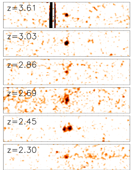
Figure 13: 2-D spectra of probable LAEs serendipitously observed in the FORS 1 long slit spectrum. The redshifts range from $z=2.30$ to 3.61. The $z=2.86$ object is LAE2138_12 previously observed also in one of the MOS slitlets (see paper I).

6 Discussion and Conclusions

The aim of our survey was to try to bridge the gap between emission selected and absorption selected galaxies at $z\approx 3$. To reach this goal we have performed the currently deepest narrow-band survey for Ly$\alpha$ emitting galaxies at $z\approx 3$ using narrow-band imaging at the VLT. Our survey was succesful in establishing the existence of a large number of galaxies below the flux limit of the Lyman-break surveys ($R=25.5$). We reach a surface density of LAEs of the order of 10 per arcmin^-2 per unit redshift. This is about an order of magnitude larger than for $R<25.5$ LBGs. It is also about a factor of two higher than that found by other deep surveys for LAEs at $z\approx 3$ (e.g. Gronwall et al., 2007). This difference mainly reflects the varitation in depth between the surveys, since if we impose a luminosity limit consistent with that of Gronwall et al. (2007) then we include only 42 of our 83 LAEs consistent which results in only about 20% more galaxies in our sample with respect to the Gronwall et al. (2007) results. This marginal overdensity we attribute to our survey targeting the environments of DLAs and Lyman-limit systems and not a blank field.

Our survey targeted three fields in which we photometrically selected 89 emission line candidates. Of these, 63 were confirmed to be emission line galaxies, however, four of the emission galaxies were foreground systems. In total we thus identified and spectroscopically confirmed 59 LAEs in the three fields. Three candidates were not observed as we could not fit them into the available masks. This corresponds to a spectroscopic confirmation rate of about 73% or 69% excluding the interlopers. Comparison of the properties of the spectroscopically confirmed and not confirmed candidates showed that the non-confirmed cases were mostly in the faint end of the narrow band magnitude range and any other related quantity (EW, Ly$\alpha$ flux and luminosity) while the broad band properties were similar for the two groups. Some of the confirmed candidates are only detected at low signal-to-noise in the spectroscopy, most noteably LAE1202_09. This LAE seems to be extended both spatially and in velocity causing the signal-to-noise in the spectroscopy to be smaller than for more compact candidates with only marginally resolved lines. Hence, some of the unconfirmed candidates maybe more broadlined systems. We conclude that the non-confirmed systems must be a mix of spurious candidates and objects with too faint emission lines to be detected by our spectroscopic follow-up. The properties of the confirmed sample of LAEs are comparable to that found by other authors as shown in Figs. 8 and 10, except being deeper. The depth of the $R$-band data does not allow for a detailed discussion, but about 90% of the selected emission line galaxies are fainter than the $R=25.5$ limit for Lyman-break surveys.

Since our survey was started in 2000 we have learned a lot more about the faint end of the luminosity function at $z\approx 3$. The study of LAEs has progressed substantially both in sample sizes and in the range of redshifts that have been probed from $z=2$ (Fynbo et al., 2002; Nilsson et al., 2008) to $z\approx 7$ (Iye et al., 2006; Ota et al., 2008). Also, using Gamma-Ray Bursts (GRBs) it has been found that a significant fraction of massive stars at these redshifts die in extremely faint galaxies, e.g. $R\approx$28 for the host galaxy of GRB030323 at $z=3.37$ (Vreeswijk et al., 2004) and $R>29.5$ for the host galaxy of GRB020124 at $z=3.20$ (Berger et al., 2002; Hjorth et al., 2003). A statistical analysis of the luminosities of GRB host galaxies again points to a large fraction of the star formation being located at the faint end of the luminosity function (Jakobsson et al., 2005; Fynbo et al., 2008). Also for continuum selected galaxies there has been significant progress. Sawicki & Thompson (2006) and Reddy & Steidel (2008) used the Lyman-break technique to push to significantly fainter limits confirming an extremely steep faint end slope.

As for the other (faint) end of the bridge, the study of the galaxy counterparts of DLAs, there has been disappointingly little progress. We still only have a few spectroscopically confirmed counterparts of high-$z$ DLAs (Møller et al., 2002, 2004; Christensen et al., 2007). An interesting development on that issue is the tentative evidence for a luminosity-metallicity relation at place at $z\approx 3$ (Møller et al., 2004; Ledoux et al., 2006) (see also Fynbo et al., 2008; Pontzen et al., 2008). This implies that targeted searches for the galaxy counterparts of metal rich DLAs could have substantially higher success rates than for randomly selected DLAs, but this remains to be confirmed. It is also consistent with the nondetection of the galaxy counterpart of the DLA towards Q2138-4427 as this DLA has a relatively low metallicity of about [Zn/H]$=-1.74$ (Ledoux et al., 2006). Another very interesting recent discovery is that of extemely faint, extended LAEs detected spectroscopically by Rauch et al. (2008) and argued by the same authors to be a population of galaxies responsible for the bulk of the DLAs (see also Barnes & Haehnelt, 2008). The argument appears very convincing, and if confirmed by more actual detections of DLA galaxy counterparts this means that we now have bridged the gap between absorption and emission selected galaxies at $z\approx$3.

Indepedent of the issue of bridging the gap between absorption and emission selected galaxies it is clear that there is a very numerous population of high-$z$ galaxies occupying the faint end of the luminosity function. There is growing evidence that this population of faint galaxies plays an important role for many important processes in the early Universe. These galaxies by far dominate the emission of ultraviolet light (e.g., Jakobsson et al., 2005; Fynbo et al., 2008) and most likely also the emission of ionizing radiation (Bianchi et al., 2001; Faucher-Giguère et al., 2008; Loeb, 2008). They also most likely contain a large fraction of the total metal budget in galaxies and are responsible for a large fraction of the enrichment of the intergalactic medium at $z\approx 3$ (e.g., Sommer-Larsen & Fynbo, 2008). Currently it is extremely difficult to infer more detailed astrophysical properties (e.g., metallicities, dust content, stellar populations, masses, etc.) for this class of objects. In a few cases like DLAs and GRB host galaxies we can infer several of these properties, but in general we cannot. With the advent of 30m class telescopes the future looks more promising.

Appendix A Data for individual LAE candidates

A.1 Spectroscopically confirmed candidates

This section gives the individual properties for the spectroscopically confirmed candidates in each of the three survey fields. The magnitudes in the tables are total magnitudes taken to be the SExtractor MAG_AUTO (Bertin & Arnouts 1996). From the total narrow-band magnitude we compute Ly$\alpha$ flux, luminosity and star formation rates. The EWs are computed based on colour indices computed from the isophotal magnitudes. The properties are derived as described in detail in Fynbo et al. (2002). For objects where the measured flux was below the $1\sigma$ level are indicated as lower/upper limits.

Table 7: Properties of the 18 confirmed LAEs in the field of BRI 1202–0725.

id	$\alpha$ (J2000)	$\delta$ (J2000)	z	N	$V$	$R$	EW0	f(Ly$\alpha$)	$L$(Ly$\alpha$)	SFR
							Å	$10^{-18}$ ergs s-1 cm-2	$10^{41}$ ergs s-1	M⊙yr-1
2	12:05:14.0	-07:40:05	3.2161	$24.31^{+0.10}_{-0.09}$	$25.05^{+0.10}_{-0.09}$	$24.98^{+0.11}_{-0.10}$	$28^{+6}_{-5}$	$48.22^{+3.96}_{-4.73}$	$43.58^{+3.58}_{-4.28}$	4.47
3	12:05:14.4	-07:42:40	3.2012	$22.19^{+0.01}_{-0.01}$	$23.43^{+0.02}_{-0.02}$	$23.63^{+0.03}_{-0.03}$	$28^{+1}_{-1}$	$340.15^{+4.56}_{-4.68}$	$307.46^{+4.12}_{-4.23}$	31.55
4	12:05:14.5	-07:40:10	3.1804	$26.45^{+0.34}_{-0.26}$	$27.36^{+0.42}_{-0.30}$	$27.81^{+0.88}_{-0.48}$	$44^{+37}_{-19}$	$6.71^{+1.41}_{-2.45}$	$6.06^{+1.28}_{-2.21}$	0.62
5	12:05:10.4	-07:45.40	3.1821	$23.25^{+0.03}_{-0.03}$	$24.62^{+0.05}_{-0.05}$	$25.07^{+0.09}_{-0.08}$	$34^{+2}_{-2}$	$127.53^{+3.12}_{-3.28}$	$115.27^{+2.82}_{-2.96}$	11.83
7	12:05:27.4	-07:40:38	3.2070	$25.25^{+0.19}_{-0.16}$	$25.92^{+0.18}_{-0.15}$	$26.21^{+0.28}_{-0.22}$	$27^{+9}_{-7}$	$20.32^{+2.76}_{-3.80}$	$18.37^{+2.50}_{-3.43}$	1.89
8	12:05:18.2	-07:42:12	3.2106	$25.67^{+0.23}_{-0.19}$	$26.93^{+0.41}_{-0.30}$	$\geq 28.05$	$64^{+44}_{-23}$	$13.73^{+2.18}_{-3.20}$	$12.41^{+1.97}_{-2.90}$	1.27
9	12:05:25.3	-07:41:13	3.2087	$25.84^{+0.24}_{-0.19}$	$26.45^{+0.21}_{-0.18}$	$26.39^{+0.23}_{-0.19}$	$28^{+16}_{-11}$	$11.76^{+1.93}_{-2.88}$	$10.63^{+1.75}_{-2.60}$	1.09
10	12:05:23.7	-07:43:44	3.2222	$25.32^{+0.18}_{-0.16}$	$26.61^{+0.26}_{-0.20}$	$26.28^{+0.28}_{-0.22}$	$38^{+18}_{-12}$	$18.94^{+2.60}_{-3.59}$	$17.12^{+2.35}_{-3.24}$	1.76
11a	12:05:18.2	-07:42:09	3.2106	$23.25^{+0.05}_{-0.05}$	$24.37^{+0.07}_{-0.07}$	$24.66^{+0.11}_{-0.10}$	$51^{+4}_{-4}$	$128.06^{+5.57}_{-6.10}$	$115.75^{+5.03}_{-5.51}$	11.88
13	12:05:18.6	-07:43:44	3.1992	$24.81^{+0.07}_{-0.07}$	$26.77^{+0.25}_{-0.20}$	$27.57^{+0.74}_{-0.44}$	$74^{+19}_{-14}$	$30.44^{+1.87}_{-2.14}$	$27.51^{+1.69}_{-1.93}$	2.82
14	12:05:12.4	-07:40:48	3.2191	$24.91^{+0.12}_{-0.11}$	$\geq 28.08$	$\geq 27.93$	$82^{+29}_{-19}$	$27.82^{+2.61}_{-3.21}$	$25.15^{+2.36}_{-2.91}$	2.58
15	12:05:31.3	-07:41:42	3.1862	$25.84^{+0.19}_{-0.16}$	$27.68^{+0.65}_{-0.41}$	$28.12^{+1.63}_{-0.62}$	$75^{+62}_{-29}$	$11.72^{+1.63}_{-2.25}$	$10.59^{+1.47}_{-2.03}$	1.09
16	12:05:13.8	-07:42:09	3.2029	$25.80^{+0.22}_{-0.19}$	$\geq 28.34$	$\geq 28.19$	$106^{+107}_{-44}$	$12.22^{+1.92}_{-2.79}$	$11.05^{+1.73}_{-2.52}$	1.13
18	12:05:15.1	-07:44:20	3.1926	$25.24^{+0.17}_{-0.15}$	$\geq 28.03$	$\geq 27.88$	$103^{+75}_{-35}$	$20.51^{+2.63}_{-3.54}$	$18.54^{+2.38}_{-3.20}$	1.90
19	12:05:22.5	-07:44:08	3.1963	$25.56^{+0.16}_{-0.14}$	$\geq 28.44$	$\geq 28.29$	$\geq 253$	$15.22^{+1.83}_{-2.41}$	$13.76^{+1.65}_{-2.17}$	1.41
21	12:05:18.6	-07:43:44	3.1978	$25.70^{+0.21}_{-0.17}$	$27.56^{+0.74}_{-0.44}$	$26.25^{+0.20}_{-0.17}$	$117^{+154}_{-50}$	$13.38^{+1.97}_{-2.79}$	$12.09^{+1.78}_{-2.52}$	1.24
22	12:05:19.1	-07:42:31	3.2057	$25.65^{+0.15}_{-0.13}$	$27.86^{+0.76}_{-0.44}$	$28.17^{+1.59}_{-0.62}$	$219^{+662}_{-104}$	$14.03^{+1.58}_{-2.05}$	$12.68^{+1.43}_{-1.85}$	1.30
23	12:05:24.1	-07:44:01	3.2203	$25.91^{+0.29}_{-0.23}$	$\geq 28.22$	$\geq 28.07$	$204^{+2165}_{-111}$	$10.98^{+2.07}_{-3.32}$	$9.93^{+1.87}_{-3.00}$	1.02

Table 8: Properties of the 18 confirmed LAEs in the field of BRI 1346–0322.

id	$\alpha$ (J2000)	$\delta$ (J2000)	z	N	$B$	$R$	EW0	f(Ly$\alpha$)	$L$(Ly$\alpha$)	SFR
							Å	$10^{-18}$ ergs s-1 cm-2	$10^{41}$ ergs s-1	M⊙yr-1
1	13:49:19.4	-03:40:30	3.1592	$24.28^{+0.12}_{-0.11}$	$26.60^{+0.46}_{-0.32}$	$\geq 27.14$	$462^{+1942}_{-240}$	$49.09^{+4.73}_{-5.86}$	$42.63^{+4.11}_{-5.09}$	4.37
2	13:49:13.7	-03:40:06	3.1307	$24.52^{+0.13}_{-0.11}$	$\geq 28.01$	$26.97^{+1.27}_{-0.57}$	$327^{+2463}_{-164}$	$39.19^{+3.85}_{-4.80}$	$34.03^{+3.35}_{-4.17}$	3.49
3	13:49:26.0	-03:39:41	3.1602	$25.62^{+0.23}_{-0.19}$	$\geq 28.49$	$\geq 27.85$	$95^{+173}_{-46}$	$14.28^{+2.29}_{-3.37}$	$12.40^{+1.99}_{-2.92}$	1.27
4	13:49:27.7	-03:39:40	3.1692	$25.36^{+0.16}_{-0.14}$	$\geq 28.60$	$\geq 27.96$	$\geq 290$	$18.14^{+2.24}_{-2.97}$	$15.75^{+1.94}_{-2.58}$	1.62
5	13:49.15.7	-03:39:37	3.1250	$24.84^{+0.16}_{-0.14}$	$27.39^{+0.85}_{-0.47}$	$\geq 27.44$	$107^{+101}_{-40}$	$29.39^{+3.49}_{-4.58}$	$25.52^{+3.03}_{-3.98}$	2.62
6	13:49:20.4	-03:39:01	3.1345	$24.82^{+0.14}_{-0.13}$	$\geq 28.17$	$25.55^{+0.20}_{-0.17}$	$\geq 496$	$29.88^{+3.29}_{-4.23}$	$25.95^{+2.86}_{-3.67}$	2.66
7	13:49:12.2	-03:38:51	3.1804	$24.16^{+0.10}_{-0.09}$	$25.40^{+0.13}_{-0.12}$	$24.69^{+0.11}_{-0.10}$	$22^{+5}_{-5}$	$54.64^{+4.52}_{-5.42}$	$47.45^{+3.93}_{-4.70}$	4.87
8	13:49:16.4	-03:38:32	3.1703	$24.36^{+0.11}_{-0.10}$	$\geq 27.96$	$\geq 27.32$	$\geq 585$	$45.68^{+4.10}_{-4.99}$	$39.66^{+3.56}_{-4.33}$	4.07
10	13:49:09.5	-03:37:23	3.1559	$24.97^{+0.17}_{-0.15}$	$26.97^{+0.49}_{-0.34}$	$26.91^{+0.99}_{-0.51}$	$64^{+55}_{-26}$	$26.08^{+3.34}_{-4.50}$	$22.65^{+2.90}_{-3.91}$	2.32
12	13:49:04.6	-03:36:35	3.1843	$25.28^{+0.15}_{-0.13}$	$26.53^{+0.19}_{-0.16}$	$25.70^{+0.14}_{-0.13}$	$35^{+10}_{-8}$	$19.48^{+2.18}_{-2.80}$	$16.92^{+1.89}_{-2.43}$	1.74
14	13:49:05.7	-03:35:03	3.1327	$24.36^{+0.14}_{-0.13}$	$25.29^{+0.14}_{-0.12}$	$24.83^{+0.15}_{-0.13}$	$24^{+7}_{-6}$	$45.54^{+4.98}_{-6.37}$	$39.55^{+4.32}_{-5.53}$	4.06
17	13:49:14.5	-03:35:26	3.1646	$22.76^{+0.05}_{-0.05}$	$24.22^{+0.07}_{-0.07}$	$23.31^{+0.05}_{-0.05}$	$29^{+3}_{-3}$	$199.39^{+8.31}_{-9.07}$	$173.14^{+7.22}_{-7.87}$	17.77
20	13:49:20.0	-03:35:52	3.1568	$25.50^{+0.24}_{-0.19}$	$\geq 28.33$	$\geq 27.70$	$\geq 264$	$16.00^{+2.61}_{-3.87}$	$13.90^{+2.27}_{-3.36}$	1.43
21	13:49:14.3	-03:36:08	3.1729	$24.29^{+0.13}_{-0.11}$	$\geq 27.75$	$25.47^{+0.27}_{-0.22}$	$168^{+434}_{-79}$	$48.57^{+4.82}_{-6.01}$	$42.18^{+4.18}_{-5.22}$	4.33
22	13:49:21.5	-03:36:09	3.1371	$25.64^{+0.20}_{-0.17}$	$27.09^{+0.31}_{-0.24}$	$24.61^{+0.05}_{-0.05}$	$43^{+15}_{-63}$	$14.06^{+1.99}_{-2.77}$	$12.21^{+1.73}_{-2.41}$	1.25
23	13:49:17.7	-03:36:33	3.1468	$24.63^{+0.13}_{-0.12}$	$\geq 28.09$	$26.48^{+0.58}_{-0.37}$	$67^{+30}_{-19}$	$35.60^{+3.58}_{-4.48}$	$30.91^{+3.11}_{-3.89}$	3.17
24	13:49:06.7	-03:36:32	3.1665	$24.85^{+0.16}_{-0.14}$	$26.55^{+0.32}_{-0.25}$	$26.05^{+0.35}_{-0.27}$	$63^{+36}_{-20}$	$29.17^{+3.46}_{-4.54}$	$25.33^{+3.00}_{-3.94}$	2.60
25	13:49:16.9	-03:36:36	3.1717	$25.54^{+0.20}_{-0.17}$	$\geq 28.56$	$\geq 27.92$	$129^{+478}_{-67}$	$15.41^{+2.21}_{-3.10}$	$13.38^{+1.92}_{-2.69}$	1.37

Table 9: Properties of the 23 confirmed LAEs in the field of Q 2138–4427.

id	$\alpha$ (J2000)	$\delta$ (J2000)	z	N	$B$	$R$	EW0	f(Ly$\alpha$)	$L$(Ly$\alpha$)	SFR
							Å	$10^{-18}$ ergs s-1 cm-2	$10^{41}$ ergs s-1	M⊙yr-1
4	21:42:12.6	-44:15:34	2.8525	$25.15^{+0.11}_{-0.10}$	$27.21^{+0.51}_{-0.34}$	$25.53^{+0.17}_{-0.15}$	$75^{+44}_{-24}$	$28.55^{+2.49}_{-3.01}$	$19.47^{+1.69}_{-2.05}$	2.00
8	21:41:56.2	-44:15:10	2.8528	$26.97^{+0.29}_{-0.23}$	$28.04^{+0.55}_{-0.36}$	$26.30^{+0.17}_{-0.15}$	$33^{+46}_{-18}$	$5.37^{+1.01}_{-1.63}$	$3.66^{+0.69}_{-1.11}$	0.38
10	21:41:54.4	-44:14:22	2.8487	$25.68^{+0.18}_{-0.15}$	$\geq 28.30$	$\geq 27.63$	$\geq 440$	$17.66^{+2.34}_{-3.18}$	$12.04^{+1.59}_{-2.17}$	1.24
11	21:42:03.7	-44:14:16	2.8563	$25.11^{+0.13}_{-0.11}$	$25.80^{+0.16}_{-0.14}$	$24.06^{+0.06}_{-0.05}$	$38^{+21}_{-13}$	$29.77^{+2.96}_{-3.70}$	$20.30^{+2.02}_{-2.52}$	2.08
12	21:42:01.9	-44:13:52	2.8576	$25.17^{+0.14}_{-0.12}$	$26.76^{+0.40}_{-0.29}$	$27.02^{+1.28}_{-0.57}$	$32^{+18}_{-11}$	$28.00^{+2.94}_{-3.73}$	$19.09^{+2.01}_{-2.54}$	1.96
14	21.41:49.0	-44:13:46	2.8463	$24.23^{+0.07}_{-0.06}$	$25.33^{+0.12}_{-0.11}$	$25.99^{+0.42}_{-0.30}$	$49^{+12}_{-9}$	$66.75^{+3.84}_{-4.34}$	$45.52^{+2.62}_{-2.96}$	4.67
16	21:41:58.9	-44:10:10	2.8561	$25.64^{+0.15}_{-0.13}$	$26.57^{+0.24}_{-0.20}$	$26.43^{+0.38}_{-0.28}$	$25^{+13}_{-9}$	$18.32^{+2.12}_{-2.75}$	$12.49^{+1.44}_{-1.88}$	1.28
17	21:42:15.5	-44:11:40	2.8532	$24.73^{+0.07}_{-0.07}$	$27.17^{+0.46}_{-0.32}$	$25.56^{+0.17}_{-0.14}$	$218^{+197}_{-74}$	$42.13^{+2.58}_{-2.95}$	$28.73^{+1.76}_{-2.01}$	2.95
18	21:41:44.7	-44:11:23	2.8627	$24.56^{+0.07}_{-0.07}$	$27.88^{+1.68}_{-0.63}$	$25.24^{+0.15}_{-0.13}$	$253^{+266}_{-90}$	$49.28^{+3.07}_{-3.51}$	$33.60^{+2.09}_{-2.39}$	3.45
19	21:42:14.9	-44:10:45	2.8542	$25.84^{+0.17}_{-0.15}$	$27.44^{+0.55}_{-0.36}$	$\geq 27.84$	$30^{+20}_{-12}$	$15.19^{+1.96}_{-2.64}$	$10.36^{+1.33}_{-1.80}$	1.06
20	21:41:58.0	-44:10:41	2.8564	$26.34^{+0.21}_{-0.18}$	$\geq 28.82$	$\geq 27.84$	$\geq 243$	$9.58^{+1.45}_{-2.07}$	$6.53^{+0.99}_{-1.41}$	0.67
21	21:41:44.0	-44:10:59	2.8525	$26.54^{+0.20}_{-0.17}$	$\geq 29.06$	$\geq 28.42$	$\geq 437$	$7.99^{+1.17}_{-1.66}$	$5.45^{+0.80}_{-1.13}$	0.56
22	21:42:11.1	-44:11:05	2.8537	$26.02^{+0.17}_{-0.15}$	$\geq 28.72$	$\geq 28.06$	$264^{+2331}_{-167}$	$12.80^{+1.65}_{-2.22}$	$8.73^{+1.12}_{-1.51}$	0.90
23	21:41:51.4	-44:11:03	2.8593	$25.77^{+0.16}_{-0.14}$	$27.67^{+0.72}_{-0.43}$	$27.43^{+1.25}_{-0.57}$	$92^{+140}_{-41}$	$16.18^{+1.98}_{-2.62}$	$11.03^{+1.35}_{-1.79}$	1.13
25	21:41:49.1	-44:11:13	2.8608	$24.94^{+0.11}_{-0.10}$	$27.02^{+0.53}_{-0.36}$	$\geq 27.43$	$40^{+18}_{-12}$	$34.87^{+3.03}_{-3.67}$	$23.78^{+2.07}_{-2.50}$	2.44
26	21:41:43.3	-44:11:25	2.8617	$24.61^{+0.08}_{-0.08}$	$27.93^{+2.33}_{-0.69}$	$25.98^{+0.34}_{-0.26}$	$86^{+37}_{-22}$	$46.95^{+3.20}_{-3.71}$	$32.01^{+2.18}_{-2.53}$	3.29
27	21:41:48.1	-44:11:19	2.8594	$25.68^{+0.16}_{-0.14}$	$\geq 28.43$	$\geq 27.77$	$167^{+1164}_{-88}$	$17.59^{+2.12}_{-2.79}$	$11.99^{+1.44}_{-1.90}$	1.23
29	21:41:49.2	-44:11:48	2.8607	$23.19^{+0.03}_{-0.03}$	$24.48^{+0.06}_{-0.06}$	$24.04^{+0.06}_{-0.06}$	$31^{+3}_{-3}$	$174.44^{+4.63}_{-4.88}$	$118.96^{+3.15}_{-3.33}$	12.21
30	21:41:59.2	-44:11:53	2.8547	$26.02^{+0.18}_{-0.15}$	$\geq 28.68$	$\geq 28.04$	$234^{+2360}_{-145}$	$12.84^{+1.67}_{-2.26}$	$8.76^{+1.14}_{-1.54}$	0.90
31	21:42:08.1	-44:12:01	2.8652	$26.56^{+0.26}_{-0.21}$	$27.27^{+0.33}_{-0.25}$	$26.64^{+0.31}_{-0.24}$	$22^{+21}_{-12}$	$7.79^{+1.35}_{-2.08}$	$5.31^{+0.92}_{-1.42}$	0.54
32	21:41:49.1	-44:13:05	2.8779	$24.91^{+0.09}_{-0.08}$	$25.93^{+0.15}_{-0.13}$	$26.04^{+0.29}_{-0.23}$	$20^{+6}_{-5}$	$35.80^{+2.64}_{-3.10}$	$24.41^{+1.80}_{-2.11}$	2.51
33	21:41:47.5	-44:13:14	2.8591	$25.01^{+0.12}_{-0.11}$	$27.25^{+0.74}_{-0.44}$	$25.92^{+0.33}_{-0.25}$	$22^{+9}_{-6}$	$32.71^{+3.09}_{-3.81}$	$22.30^{+2.11}_{-2.60}$	2.29
36	21:41:59.3	-44:13:18	2.8586

A.2 Candidates not confirmed by the available spectroscopy

This section gives the properties of the emission line candidates for which the nature could not be assessed through the available spectroscopic data. The properties are measured as detailed in the previous section. The restframe EWs are given assuming the redshift corresponding to the central wavelength of the filter.

Table 10: Properties of the non-confirmed LAE candidates.

id	$\alpha$ (J2000)	$\delta$ (J2000)	N	$V$/$B$	$R$	EW0	f(Ly$\alpha$)	$L$(Ly$\alpha$)	SFR
						Å	$10^{-18}$ ergs  s-1 cm-2	$10^{41}$ ergs  s-1
BRI 1202–0725
1	12:05:31.5	-07:41:16	$26.05^{+0.29}_{-0.23}$	$26.53^{+0.23}_{-0.19}$	$26.26^{+0.20}_{-0.17}$	$21^{+13}_{-9}$	$9.73^{+1.84}_{-2.96}$	$8.79^{+1.66}_{-2.67}$	0.90
6	12:05:31.2	-07:42:48	$26.42^{+0.36}_{-0.27}$	$26.99^{+0.30}_{-0.24}$	$27.30^{+0.51}_{-0.34}$	$27^{+19}_{-12}$	$6.87^{+1.50}_{-2.68}$	$6.21^{+1.36}_{-2.42}$	0.64
12	12:05:27.7	-07:42:38	$26.55^{+0.37}_{-0.28}$	$26.86^{+0.24}_{-0.20}$	$26.47^{+0.19}_{-0.16}$	$42^{+34}_{-18}$	$6.14^{+1.38}_{-2.50}$	$5.55^{+1.25}_{-2.26}$	0.57
17	12:05:10.6	-07:41:06	$26.56^{+0.22}_{-0.18}$	$27.89^{+0.42}_{-0.30}$	$\geq 28.98$	$71^{+107}_{-35}$	$6.04^{+0.93}_{-1.34}$	$5.46^{+0.84}_{-1.21}$	0.56
20	12:05:31.9	-07:41:30	$26.85^{+0.22}_{-0.18}$	$\geq 29.42$	$28.63^{+0.87}_{-0.48}$	$186^{+2195}_{-109}$	$4.62^{+0.71}_{-1.02}$	$4.17^{+0.64}_{-0.93}$	0.43
24	12:05:21.0	-07:45:01	$26.97^{+0.50}_{-0.34}$	$27.06^{+0.25}_{-0.21}$	$26.76^{+0.22}_{-0.18}$	$74^{+70}_{-32}$	$4.17^{+1.13}_{-2.45}$	$3.76^{+1.02}_{-2.22}$	$0.39$
25	12:05:28.3	-07:40:54	$26.88^{+0.36}_{-0.27}$	$28.29^{+0.81}_{-0.46}$	$27.46^{+0.36}_{-0.27}$	$118^{+370}_{-61}$	$4.51^{+0.98}_{-1.74}$	$4.07^{+0.89}_{-1.58}$	0.42
BRI 1346–0322
9	13:49:10.5	-03:38:21	$25.02^{+0.17}_{-0.15}$	$26.42^{+0.26}_{-0.21}$	$24.39^{+0.07}_{-0.06}$	$28^{+11}_{-8}$	$24.86^{+3.16}_{-4.24}$	$21.59^{+2.75}_{-3.68}$	2.22
11	13:49:27.3	-03:33:58	$25.76^{+0.24}_{-0.20}$	$27.43^{+0.50}_{-0.34}$	$\geq 27.94$	$62^{+62}_{-27}$	$12.57^{+2.10}_{-3.16}$	$10.92^{+1.83}_{-2.74}$	1.12
13	13:49:26.4	-03:34:02	$25.86^{+0.28}_{-0.22}$	$26.90^{+0.30}_{-0.24}$	$25.98^{+0.21}_{-0.18}$	$93^{+130}_{-41}$	$11.42^{+2.12}_{-3.36}$	$9.92^{+1.84}_{-2.92}$	1.02
15a	13:49:29.4	-03:35:08	$25.36^{+0.23}_{-0.19}$	$26.29^{+0.22}_{-0.18}$	$24.60^{+0.08}_{-0.07}$	$32^{+18}_{-12}$	$18.08^{+2.89}_{-4.24}$	$15.70^{+2.51}_{-3.68}$	1.61
18a	13:49:29.2	-03:35:31.2	$25.23^{+0.20}_{-0.17}$	$26.53^{+0.28}_{-0.22}$	$24.57^{+0.07}_{-0.07}$	$34^{+22}_{-13}$	$20.51^{+2.98}_{-4.19}$	$17.81^{+2.58}_{-3.64}$	1.83
26	13:49:19.4	-03:37:01	$25.60^{+0.17}_{-0.14}$	$27.14^{+0.29}_{-0.23}$	$25.20^{+0.08}_{-0.07}$	$26^{+13}_{-9}$	$14.61^{+1.81}_{-2.41}$	$12.68^{+1.57}_{-2.09}$	1.30
Q 2138–4427
1	21:41:44.6	-44:16:07	$26.61^{+0.23}_{-0.19}$	$28.34^{+0.91}_{-0.49}$	$25.44^{+0.09}_{-0.08}$	$31^{+31}_{-15}$	$7.45^{+1.20}_{-1.77}$	$5.08^{+0.82}_{-1.21}$	0.52
2	21:41:53.0	-44:15:42	$25.31^{+0.10}_{-0.09}$	$26.15^{+0.14}_{-0.12}$	$24.71^{+0.06}_{-0.06}$	$18^{+6}_{-5}$	$24.73^{+1.93}_{-2.29}$	$16.86^{+1.32}_{-1.56}$	1.73
3	21:41:46.2	-44:15:38	$25.55^{+0.16}_{-0.14}$	$27.06^{+0.44}_{-0.31}$	$25.32^{+0.14}_{-0.12}$	$35^{+19}_{-12}$	$19.75^{+2.35}_{-3.09}$	$13.47^{+1.60}_{-2.11}$	1.38
5	21:42:12.1	-44:15:32	$26.71^{+0.21}_{-0.17}$	$27.59^{+0.32}_{-0.25}$	$26.41^{+0.17}_{-0.15}$	$23^{+19}_{-11}$	$6.79^{+1.01}_{-1.43}$	$4.63^{+0.69}_{-0.98}$	0.48
6	21:42:14.8	-44:15:15	$26.72^{+0.26}_{-0.21}$	$27.49^{+0.35}_{-0.27}$	$26.08^{+0.15}_{-0.14}$	$29^{+38}_{-17}$	$6.72^{+1.17}_{-1.80}$	$4.58^{+0.80}_{-1.23}$	0.47
7	21:42:12.6	-44:15:11	$26.31^{+0.22}_{-0.18}$	$27.50^{+0.45}_{-0.32}$	$25.57^{+0.12}_{-0.11}$	$29^{+27}_{-14}$	$9.82^{+1.51}_{-2.19}$	$6.69^{+1.03}_{-1.49}$	0.69
9	21:42:10.5	-44:14:38	$26.33^{+0.17}_{-0.15}$	$27.66^{+0.40}_{-0.29}$	$25.72^{+0.11}_{-0.10}$	$50^{+59}_{-23}$	$9.62^{+1.24}_{-1.67}$	$6.56^{+0.85}_{-1.14}$	0.67
13	21:42:15.5	-44:13:51	$26.41^{+0.17}_{-0.15}$	$27.21^{+0.24}_{-0.20}$	$26.16^{+0.15}_{-0.13}$	$20^{+13}_{-9}$	$9.00^{+1.15}_{-1.54}$	$6.14^{+0.78}_{-1.05}$	0.63
15	21:42:12.9	-44:13:35	$25.97^{+0.18}_{-0.16}$	$27.43^{+0.50}_{-0.34}$	$26.03^{+0.22}_{-0.18}$	$35^{+48}_{-19}$	$13.41^{+1.81}_{-2.49}$	$9.15^{+1.24}_{-1.69}$	0.94
34	21:42:12.6	-44:11:36	$26.01^{+0.22}_{-0.18}$	$27.08^{+0.41}_{-0.30}$	$25.71^{+0.19}_{-0.16}$	$24^{+30}_{-14}$	$13.02^{+2.04}_{-2.97}$	$8.88^{+1.39}_{-2.02}$	0.91
35	21:42:12.6	-44:10:10	$26.52^{+0.23}_{-0.19}$	$28.09^{+0.75}_{-0.44}$	$26.26^{+0.20}_{-0.17}$	$41^{+50}_{-20}$	$8.08^{+1.31}_{-1.94}$	$5.51^{+0.89}_{-1.32}$	0.57