,
Enhancing the capabilities of LIGO time-frequency plane searches through clustering
Abstract
One class of gravitational wave signals LIGO is searching for consists of short duration bursts of unknown waveforms. Potential sources include core collapse supernovae, gamma ray burst progenitors, and mergers of binary black holes or neutron stars. We present a density-based clustering algorithm to improve the performance of time-frequency searches for such gravitational-wave bursts when they are extended in time and/or frequency, and not sufficiently well known to permit matched filtering. We have implemented this algorithm as an extension to the QPipeline, a gravitational-wave data analysis pipeline for the detection of bursts, which currently determines the statistical significance of events based solely on the peak significance observed in minimum uncertainty regions of the time-frequency plane. Density based clustering improves the performance of such a search by considering the aggregate significance of arbitrarily shaped regions in the time-frequency plane and rejecting the isolated minimum uncertainty features expected from the background detector noise. In this paper, we present test results for simulated signals and demonstrate that density based clustering improves the performance of the QPipeline for signals extended in time and/or frequency.
pacs:
04.80.Nn, 07.05.Kf, 95.55.Ym, 95.75.Pq1 Introduction
The first generation of interferometric gravitational wave detectors have now collected data at their design strain sensitivities [1, 2, 3, 4, 5, 6], and an improved generation of detectors [7, 8] is already under development. Even at this unprecedented level of sensitivity, potentially detectable signals from astrophysical sources are expected to be at or near the limits of detectability, requiring carefully designed search algorithms in order to identify and distinguish them from the background detector noise. In this study, we focus on the problem of detecting the specific class of gravitational wave signals known as gravitational-wave bursts (GWBs). These are signals lasting from a few milliseconds to a few seconds, for which we do not have sufficient theoretical understanding or reliable models to predict a waveform. This includes signals from the merger of binary compact objects, asymmetric core collapse supernovae, the progenitors of gamma ray bursts, and possibly unexpected sources.
Since accurate waveform predictions do not exist for GWBs, the typical method to identify them is to project the data under test onto a convenient basis of abstract waveforms that are chosen to cover a targeted region of the time-frequency plane, and then identify regions of this search space with statistically significant excess signal energy [9]. In this study, we focus on one such burst search algorithm, the QPipeline [10], which first projects the data under test onto an overlapping basis of Gaussian enveloped sinusoids characterized by their center time, center frequency, and quality factor. A trigger is recorded whenever this projection exceeds a threshold value, with the magnitude of the projection indicating the significance of the trigger. Since the triggers are considered separately, the existing algorithm currently under-reports the total energy and true significance of those signals that are extended in time and/or frequency, since they have a significant projection onto multiple independent basis functions. Since GWB signals with such extended features are commonly observed in simulations of core collapse supernovae, the mergers of binary compact objects, and instabilities of spinning neutron stars, there are good reasons to try to improve the sensitivity of the search algorithm to such sources.
To improve the sensitivity of the QPipeline to signals that are extended in time and/or frequency, we have investigated extensions to the QPipeline that also consider the combined statistical significance of arbitrarily shaped clusters of projections in the time-frequency plane. Although a number of clustering algorithms are commonly available [11], this work focuses on a density based clustering algorithm due to its ability to also decrease the false detection probability of GWB searches by rejecting isolated single projection events associated with noise fluctuations. In this paper we present the details of a density based clustering algorithm implementation as an extension to the QPipeline, and demonstrate the resulting improved performance of the QPipeline for signals that are extended in time and/or frequency.
The paper is structured as follows. Section 2 briefly describes the QPipeline burst search algorithm. Section 3 considers the motivations for clustering and surveys some of the available approaches. Section 4 presents the details of the proposed density based clustering algorithm. Section 5 demonstrates the benefit of the proposed approach for detecting simulated gravitational wave bursts of various waveforms. Finally, in section 6, we present our conclusions and discuss possible future investigations.
2 The QPipeline burst search algorithm
The QPipeline is an analysis pipeline for the detection of GWBs in data from interferometric gravitational wave detectors [10]. It is based on the Q-transform [12], a multi-resolution time-frequency transform that projects the data under test onto the space of Gaussian windowed complex exponentials characterized by a center time , center frequency , and quality factor .
| (1) |
The space of Gaussian enveloped complex exponentials is an overlapping basis of waveforms, whose duration and bandwidth , defined as the standard deviation of the squared Gaussian envelope in time and frequency, have the minimum possible time-frequency uncertainty, , where .
There is good reason to select an overlapping basis of multi-resolution minimum-uncertainty functions. Absent detailed knowledge of the gravitational waveform, such a basis provides the tightest possible constraints on the time-frequency area of unmodeled signals, permitting the time-frequency distribution of signal energy to be non-coherently reconstructed while incorporating as little noise energy as possible. A choice of basis that does not have minimum time-frequency uncertainty would typically include more noise than necessary, decreasing signal to noise ratio. The exception would be a restricted search for a known set of waveforms, in which a matched filter search, where the template matches the target signal, would be optimal. This type of restricted search is not the focus of this paper. Another benefit of the tighter time-frequency constraints afforded by a multi-resolution sine-Gaussian template bank is the decreased likelihood for false coincidences, when testing for coincidence between multiple detectors.
In practice, the Q transform is evaluated only for a finite number of basis functions, also referred to here as templates or tiles. These templates are selected to cover a targeted region of signal space, and are spaced such that the fractional signal energy loss due to the mismatch , , and between an arbitrary basis function and the nearest measurement template,
| (2) |
is no larger than . This naturally leads to a tiling of the signal space that is logarithmic in Q, logarithmic in frequency, and linear in time.
The statistical significance of Q transform projections are given by their normalized energy , defined as the ratio of squared projection magnitude to the mean squared projection magnitude of other templates with the same central frequency and . For the case of ideal white noise, is exponentially distributed, and related to the matched filter SNR [13] by the relation
| (3) |
The QPipeline consists of the following steps. The data is first whitened by zero-phase linear predictive filtering [14, 10]. Next, the Q-transform is applied to the whitened data, and normalized energies are computed for each measurement template. Templates with statistically significant signal content are then identified by applying a threshold on the normalized energy. Finally, since a single event may potentially produce multiple overlapping triggers due to the overlap between measurement templates, only the most significant of overlapping templates are reported as triggers. As a result, the QPipeline is effectively a templated matched filter search [13] for signals that are Gaussian enveloped sinusoids in the whitened signal space.
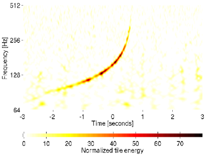
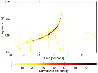
Figure 1 shows an example of the QPipeline applied to the inspiral phase of a simulated binary neutron star coalescence signal injected into typical single detector LIGO data with an SNR of 48.2.
3 Motivations and options for clustering
Currently, the QPipeline considers the significance of triggers independently. The detectability of a particular GWB signal therefore depends upon its maximum single projection onto the space of Gaussian enveloped sinusoids. As a result, the QPipeline is most sensitive to signals with near minimum time-frequency uncertainty, and less sensitive to signals that are extended in time and/or frequency such that their energy is spread across multiple non-overlapping basis functions. For example, the detectability of the simulated inspiral signal shown in Figure 1 is currently determined by the single most significant tile near the center of the signal, which has a single tile SNR of 12.7. This is significantly less than the SNR of 48.2 that is recovered by a matched filter search tuned for this waveform.
Although the above example focuses on binary neutron star inspiral waveforms, matched filter search methods are more appropriate to search for such signals, since there waveform is well understood [15, 16, 17, 18]. We focus on them here only because they represent an astrophysically interesting example case of a signal which is extended in time and frequency. The QPipeline is not intended to search for inspiral signals, but instead focuses on the search for other transient sources such as the less well understood merger phase of coalescing binary compact objects, core collapse supernovae, and instabilities in spinning neutron stars, many of which are also expected to produce waveforms that are extended in time and/or frequency [19, 20, 21, 22]. As a result, we seek a method to improve the sensitivity of the QPipeline to signals that are extended in time and/or frequency that is applicable to the general case of astrophysically unmodeled bursts, and is not specific to any one particular waveform.
An obvious solution is to simultaneously consider the aggregate significance of all tiles that comprise the signal. This requires an approach that identifies clusters of related tiles in the time-frequency plane. In this context, we define clustering as the grouping of the set of all significant QPipeline tiles into subsets, such that all tiles within a subset are closely related by their relative distance in the time-frequency plane.
There are many different clustering methods available; however, they all tend to fall into three categories [11].
Partitioning methods The classical example of a partitioning method is the K-means algorithm [24]. In K-means clustering, a fixed number of clusters presupposed, and an initial guess to partition objects into these clusters is made. A centroid is computed for each cluster, and the total sum distance of all objects from their cluster centroid is computed as a figure of merit. K-means iteratively reassigns objects to different clusters until this figure of merit is minimized.
There are a number of drawbacks to the K-means approach, as described in [24, 11]. The first is that it presupposes a fixed number of clusters, though there are variations that allow the number of clusters to change [25]. The other difficulty with the K-means approach is the tendency to produce spherical or ellipsoidal clusters rather than more complicated arbitrary shapes. This is acceptable for some signal morphologies but not so in general. For example, the signal expected from inspiralling binary compact objects, which is long and extended in time and frequency, would not be easily identified by K-means clustering [25]. A third difficulty with the K-means approach is the sensitivity to the initial guess, and the possibility of the algorithm to identify a local rather than global minimum [11].
Hierarchical methods This type of clustering algorithm first evaluates the pairwise difference between all objects, then arranges them into a tree structure, where each object to be clustered is a leaf [26]. In the agglomerative hierarchical approach, the tree is constructed in levels. At each level, the closest pair of leaves and/or branches is merged, with the th level representing a cluster of all objects. A cluster is formed by cutting this tree based on some criteria such as a maximum distance or the inconsistency between the distance between cluster leaves or branches and the distance to the next closest leaf or branch.
Hierarchical clustering has the flexibility of producing arbitrary numbers of clusters with arbitrary shape, and is therefore more applicable to the problem of clustering in time, frequency, and Q for gravitational-wave burst detection.
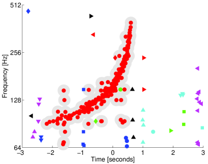
The left panel from Figure 2 shows an example of hierarchical clustering, implemented using the functions “linkage” and “cluster” from MATLAB Statistics Toolbox 111Statistics Toolbox Software Version ; applied to the detection of a simulated binary neutron star inspiral signal. The draw back to this approach is that it presupposes that every data point must be included in one cluster or another, even if a cluster is to be constituted of only one data point. As a result, it produces a large number of insignificant clusters and tends to build clusters of unrelated data points.
Density based methods Density based clustering [23] is a variation on the hierarchical clustering approach. Instead of constructing a tree structure, density based clustering starts with single object and iteratively adds objects to that cluster using a predefined set of criteria based on the density of objects within a given neighborhood radius, until the criteria is no longer met and all objects have been tested.
Like other hierarchical methods, density based methods also allow an arbitrary number of clusters as well as arbitrary cluster shape. They also have the advantage of rejecting single isolated data points that are not potentially related with a large number of points. Thus this method only produces clusters with multiple data points and can successfully exclude unrelated points from a cluster. For this reason, we have focused on density based methods in this work.
4 Density based clustering algorithm
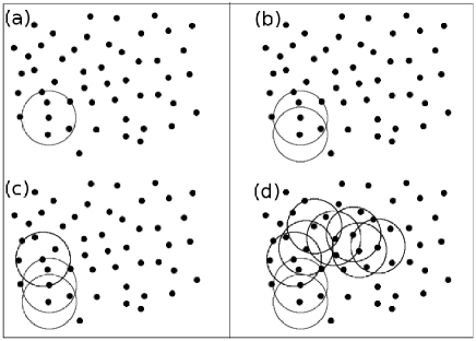
Density based clustering [23] facilitates searches for signals of unknown shape. It does not clutter the output with a list of numerous noise related clusters that contain just a few significant data-points. The algorithm looks for neighbors of those points that have at least a given number of neighboring points within a given distance on the time-frequency plane, and forms clusters of data-points that can be related through their common neighbors. Our implementation of density based clustering algorithm takes two parameters: minimum neighbor number and neighborhood radius, and it considers each tile produced by QPipeline as a data-point.
Density based clustering first finds a tile’s nearest neighbors, then that neighbors’ neighbors, and so on. In the left panel of Fig. 3, (a) shows data points before clustering. If the density of data points within a given distance around a point is above a given threshold to form a cluster, that point becomes a cluster seed (b). Neighboring data points having a sufficient number of neighbors are then included in the cluster (c). This process repeats as long as data points with sufficient number of neighbors are found (d).
Any clustering algorithm requires measurement of the pairwise distances between all data points; in our case, the pairwise distance between all tiles produced by QPipeline. Unfortunately, the tiles have varied shapes, which makes measurement of distance between any pair of tiles somewhat difficult. We have implemented a simple distance metric that addresses the issue of varied tile shapes. For a pair of tiles with center times and , center frequencies and , Q of and , and normalized energy of and , the distance on the time-frequency plane D is measured from the following relations:
| (4) |
| (5) |
| (6) |
where is the distance along the time scale, is the distance along the frequency scale, is the scale factor on the time scale, is the scale factor on the frequency scale, and are durations, and and are bandwidths.
The parameter is a tuning parameter that determines the relative importance of distance in frequency versus distance in time. It was determined empirically that when , the best results were achieved for the extended signals considered in Section 5 as measured by the receiver operating characteristic (ROC) curves presented there.
The mismatch metric in Equation 2 can also be used [10] for this purpose. However, in this initial study we have chosen to use the simpler approach of Equations 4, 5, and 6, and leave the possibility of using Equation 2 for future study.
The minimum neighbor number determines which tiles are to be considered as potential cluster seeds, and which ones are to be excluded from the clustering process entirely because they do not have a sufficient number of neighboring tiles. A minimum neighbor number that is too low may result in too many clustering seeds, potentially producing a large number of clusters, whereas a minimum neighbor number that is too high may result in the exclusion of too many tiles.
The neighborhood radius indicates the distance the algorithm searches from a tile in order to find neighboring tiles, and therefore determines the maximum gap over which the algorithm can cluster. A neighborhood radius that is too low may result in a large number of small clusters, whereas a neighborhood radius that is too high may result in the creation of one large cluster consisting of all significant tiles.
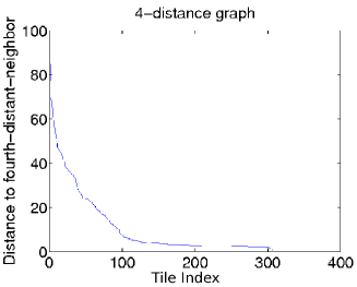
The exact numerical value of the neighborhood radius depends on the minimum neighbor number and the distance metric used. We have experimented by varying the minimum neighbor number from 1 to 8, and found that the best results were achieved with a minimum neighbor number of 4, as measured by the ROC curves in Section 5. The value of the neighborhood radius was then determined using the 4-distance graph in right panel of Figure 3. The 4-distance graph shows the number of tiles on the x-axis whose fourth closest neighbor is less than the distance shown on the y-axis. Motivated by the 4-distance plot, we experimented by varying the neighborhood radius between 3 and 12, and found that a value of 8 produced the best results based on the ROC curves in Section 5.
A flowchart of the density based clustering algorithm is shown in Figure 4. The main clustering function first uses the distance function to measure pairwise distance between all tiles, and then calls the expandCluster function, which recursively calls itself, to incorporate more tiles into the each cluster. The algorithm as presented here was implemented in MATLAB 222MATLAB Version ; .
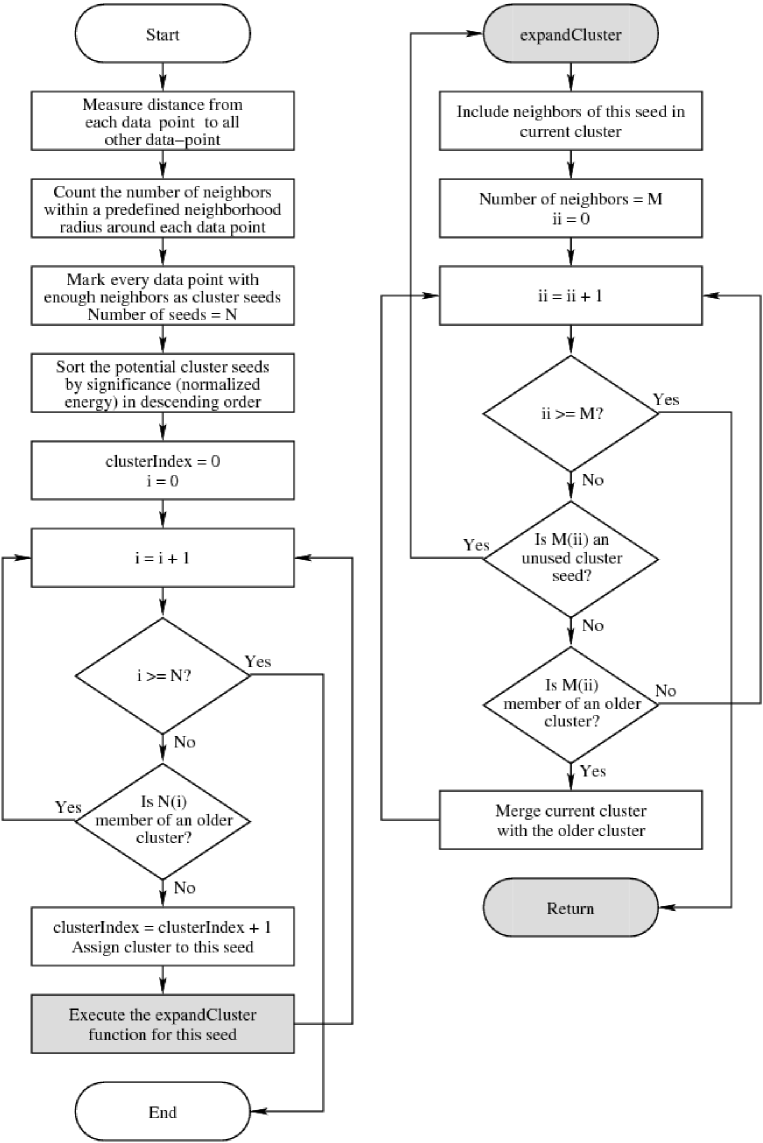
Clustering starts with the highest energy tile that has a sufficient number of neighbors, and then proceeds to the next significant tile that also has a sufficient number of neighboers, and is not already assigned to a cluster. If any qualifying member of the current cluster is found to be already belong to another cluster, the two clusters are merged. Thus, regardless of which tile the algorithm starts clustering from, it will always find the same clusters for a given set of tiles. For speed optimization, though, our density based clustering function starts with the more significant tiles first.
The computational cost of the resulting algorithm is dominated by the cost of computing the distance between all pairs of tiles, where is the number of tiles. In practice, clustering is applied separately to the 1 minute data blocks used by the QPipeline analysis. This is more than sufficient to detect clusters up to a few seconds in duration, the typical limit of gravitational wave burst searches. At the typical 1 Hz single detector false rate, the resulting computational cost due to clustering is small compared to that of the rest of the search.
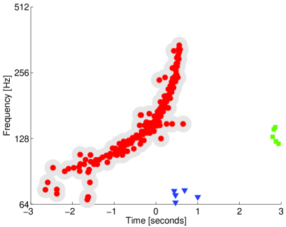
The right panel of Fig. 2 shows an example cluster constructed using the proposed density based clustering algorithm. It can be seen that the algorithm has clustered together the most significant part of the previously discussed injection successfully. In addition, almost all of the spurious noise tiles have also been removed. While the high-frequency end of the signal has been lost, that part contains very little energy, and does not significantly contribute to the significance of the detected trigger.
5 Evaluating performance improvements
We have evaluated our implementation of density based clustering by measuring its effect on the detection of simulated signals injected into typical single detector LIGO data, and its effect on the rate of false detections.
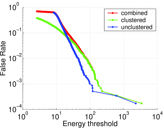
In order to evaluate the false detection rate, the QPipeline was first applied to single detector data without injected signals. This was performed both with and without clustering. Since detectable GWB events are expected to be extremely rare in the few hours of data considered here, and since we have set our thresholds to yield event rates up to 1 Hz and not demanded coincidence between multiple detectors to reject false events, we can safely identify false events as those events in a given data stretch whose total normalized energy exceeded a specified detection threshold. Three sets of false events were identified: unclustered events, clustered events, and combined events formed by the union of unclustered and clustered events. The resulting false event rates as a function of detection threshold are shown in Figure 5.
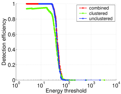
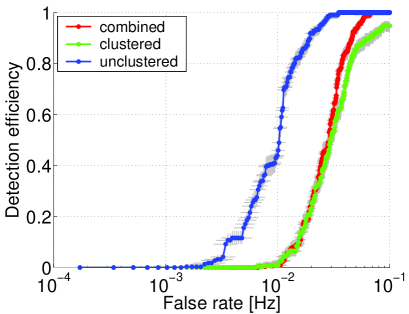
An adverse effect of using density based clustering is the occasional rejection of highly localized signals, regardless of the detection threshold. This is due to the tendency of density based clustering to exclude isolated triggers. This is also evident in Figure 6, where detection efficiency of sinusoidal Gaussians does not converge to 100 percent for the case of clustered triggers. To overcome this, we have also considered the performance of a search consisting of the union of both clustered and unclustered triggers, and compared it with that for clustered triggers and unclustered triggers only. The resulting sinusoidal Gaussian combined detection efficiency for a given energy-threshold is then comparable to that of the unclustered case, as shown in Figure 6.
Another possible solution to this problem is to reduce the required number of tiles within the neighborhood radius to zero, permitting single tile clusters. Classical hierarchical clustering also provides an alternative to density based clustering that permits single tile clusters. Since the focus of this paper is on improved performance for signals that are extended in time and/or frequency, we have not considered either of these alternative choices here.
The lower false event rate observed in Figure 5 for clustered triggers at low detection thresholds is associated with the rejection of isolated noise events as described in Section 4. At high detection thresholds, the opposite is true. The presence of transient non-stationary “glitches” in the data that are extended in time and/or frequency cause the false event rate of clustered triggers to exceed that of unclustered triggers.
| Inspiral signals, SNR 25 | |
 |
 |
| White noise burst signals, SNR 25 | |
 |
 |
| Sinusoidal Gaussian signals, SNR 10 | |
 |
 |
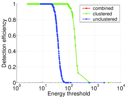
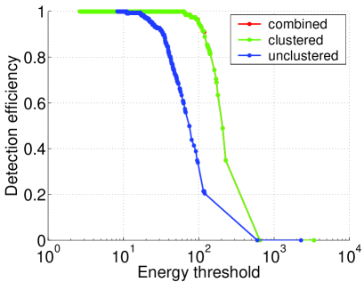
To evaluate the effect of clustering on the detection of signals, we next applied the QPipeline to the recovery of simulated signals injected into the same single detector data. Again, this was performed both with and without clustering. Injections were identified as detected if a event was observed above the detection threshold within 1 second of the time of the injected signal. We define the detection efficiency as the fraction of injection signals that were correctly detected, and evaluate this efficiency as a function of detection threshold for signals injected at a constant signal to noise ratio.
In order to characterize the performance of density based clustering for a variety of signal morphologies, we have repeated this analysis for five different waveform families. They include simple Gaussian pulses, sinusoidal Gaussian pulses, and the fundamental ring down mode of perturbed black holes, which represent signals that are highly localized in the time-frequency plane; and the inspiral phase of coalescing binary compact objects and band-limited time-windowed white noise bursts, which are both extended in the time-frequency plane. Within each waveform family, signals were injected with random parameters such as time, frequency, duration, bandwidth, mass, etc.
Among non-localized signals, inspirals and white noise bursts represent two extremes: white noise bursts fill a large time-frequency region, whereas inspirals, while extended in time and frequency, still only occupy a small portion of a time-frequency region. Three of the waveform families are ad-hoc: simple Gaussian pulses, sinusoidal Gaussian pulses, and white noise bursts. Two of the waveform families were astrophysical: inspirals and ringdowns. While we are not designing a search to only target known waveforms such as ringdowns and inspirals, they are nonetheless also a useful test case because they are astrophysically motivated and because they can form a basis for comparison with other existing searches, including matched filter searches.
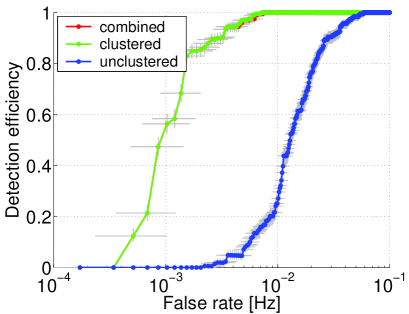
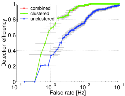
On the left side panels of Figure 6, we present the resulting detection efficiency as a function of detection threshold for three of the waveform families that we have considered, representing both ad-hoc and astrophysical, as well as localized and extended. On the right side panels of Figure 6, we report the receiver operator characteristic (ROC) for each waveform, which combines the measured false rate from Figure 5 with the detection efficiencies from the left side panels.
The results indicate that for the extended waveforms, such as the inspiral and noise burst waveforms, clustering increases search efficiency and significantly improves the resulting ROC by approximately an order of magnitude in false rate. The primary reason for this improved performance is the increase in measured signal energy due to clustering, which is evident as increased detection efficiency in the left hand side of Figure 6.
Although clustering provides a marked improvement for the detection of signals that are extended in time and frequency, Figure 6 indicates that clustering also adversely impacts the performance of the search for localized waveforms. In particular, the ROC for sinusoidal Gaussians is worse by roughly a factor of 3 in false rate due to the addition of clustering. The primary cause of this decreased performance is the higher false event rate, which is due to the increased significance of detector glitches after clustering, and is evident in Figure 5. For signals that are extended in time and/or frequency this higher false event rate is more than compensated by the significant improvement in detection efficiency, but for more localized signals there is no improvement in detection efficiency to compensate for the increased false rate. In practice, we expect the presence of such detector glitches to be largely mitigated by the requirement of a coincident and consistent observation of a gravitational wave in multiple detectors, as well as the absence of a signal in environmental monitors. As a result, the decreased performance for localized signals may also be somewhat mitigated.
6 Conclusions
A density based method for clustering the measurements from neighboring or overlapping basis functions has been employed to more efficiently detect GWB signals that are extended in time and/or frequency, and not well represented by QPipeline’s particular choice of basis. The method is capable of identifying an arbitrary number of clusters of arbitrary shape and size, while also rejecting spurious noise triggers, and does not significantly increase the computational cost of the overall QPipeline search.
The proposed clustering algorithm itself is not specific to the QPipeline. Similar improvements are expected when applied to other time-frequency searches for gravitational wave bursts. In particular, the algorithm described here has already been applied to the search for bursts from the soft gamma repeaters using the flare pipeline [27, 28, 29]. For estimating upper limits, the flare pipeline initially performed a simple sum over all frequency bins to measure the total signal energy of a trigger. The use of density based clustering instead improved the flare pipeline’s upper limit estimate for 100 ms long white noise bursts in the frequency band from 64 to 1024 Hz by 42%. No improvement was observed for 22 ms long white noise bursts in the band from 100 to 200 Hz, but such signals are fairly localized in the time-frequency plane. These results are consistent with our conclusion that density based clustering is only beneficial when searching for extended signals.
Our implementation of density based clustering is already implemented as part of the QPipeline, which has now been incorporated into the -Pipeline [30] for use in future GWB searches.
A number of issues remain open for future investigation. This paper has focused only on single detector data. We have left a study of the effect of density based clustering on multi-detector GWB searches as a subject for future investigation. In Equation 4, we have proposed one possible distance metric. A study of other distance metrics, in particular ones based on the mismatch metric of Equation 2 is also possible. A more in depth study of hierarchical clustering methods, and comparison with the proposed density based method, as well as previously proposed methods [31, 32, 33] is also recommended. Finally, the application of clustering to astrophysical parameter estimation in the event of a detection also warrants further investigation.
References
References
- [1] D. Sigg and the LIGO Scientific Collaboration. Status of the LIGO detectors. Classical and Quantum Gravity, 25(11):114041–+, June 2008.
-
[2]
LIGO Scientific Collaboration.
LIGO detector noise curves during the S5 run.
http://www.ligo.caltech.edu/docs/G/G060009-03/, 2007. - [3] Acernese, F. et al. Classical and Quantum Gravity, 23:S63, 2006.
- [4] Lück, H. et al. Classical and Quantum Gravity, 23:S71, 2006.
- [5] F. Beauville et al. Benefits of joint LIGO - Virgo coincidence searches for burst and inspiral signals. Journal of Physics Conference Series, 32:212–222, March 2006.
- [6] Abbott B. et al. Detector description and performance for the first coincidence observations between LIGO and GEO. Nuclear Instruments and Methods in Physics Research A, 517:154–179, January 2004.
- [7] S. Waldman R. Adhikari, P. Fritschel. Enhanced LIGO. 2006. LIGO technical document T060156.
- [8] http://www.astro.cf.ac.uk/geo/advligo/.
- [9] Warren G. Anderson, Patrick R. Brady, Jolien D. E. Creighton, and Eanna E. Flanagan. An excess power statistic for detection of burst sources of gravitational radiation. Phys. Rev., D63:042003, 2001.
- [10] S. K. Chatterji. The search for gravitational wave bursts in data from the second LIGO science run. PhD thesis, Massachusetts Institute of Technology, 2005.
- [11] A. K. Jain, M. N. Murty, and P. J. Flynn. Data clustering: a review. ACM Comput. Surv., 31(3):264–323, 1999.
- [12] Shourov Chatterji, Lindy Blackburn, Gregory Martin, and Erik Katsavounidis. Multiresolution techniques for the detection of gravitational-wave bursts. Class. Quantum Grav., 21:S1809–S1818, 2004.
- [13] D. Dewey. Analysis of gravity wave antenna signals with matched filter techniques. Molecular Genetics and Metabolism, pages 581–590, 1986.
- [14] J. Makhoul. Linear prediction: A tutorial review. Proc. IEEE, 63, 1975.
- [15] M. V. van der Sluys, C. Röver, A. Stroeer, V. Raymond, I. Mandel, N. Christensen, V. Kalogera, R. Meyer, and A. Vecchio. Gravitational-Wave Astronomy with Inspiral Signals of Spinning Compact-Object Binaries. Astrophysics Letters, 688:L61–L64, December 2008.
- [16] M. van der Sluys, V. Raymond, I. Mandel, C. Röver, N. Christensen, V. Kalogera, R. Meyer, and A. Vecchio. Parameter estimation of spinning binary inspirals using Markov chain Monte Carlo. Classical and Quantum Gravity, 25(18):184011–+, September 2008.
- [17] R. Gouaty and for the LIGO Scientific Collaboration. Detection confidence tests for burst and inspiral candidate events. Classical and Quantum Gravity, 25(18):184006–+, September 2008.
- [18] B. Abbott et al. Search of S3 LIGO data for gravitational wave signals from spinning black hole and neutron star binary inspirals. Phys. Rev. D, 78(4):042002–+, August 2008.
- [19] T. Baumgarte et al. Learning about compact binary merger: the interplay between numerical relativity and gravitational-wave astronomy. ArXiv General Relativity and Quantum Cosmology e-prints, December 2006.
- [20] T. Z. Summerscales et al. Maximum Entropy for Gravitational Wave Data Analysis: Inferring the Physical Parameters of Core-Collapse Supernovae. ArXiv e-prints, 704, April 2007.
- [21] C. D. Ott. The Gravitational Wave Signature of Core-Collapse Supernovae. ArXiv e-prints, September 2008.
- [22] H. Dimmelmeier, C. D. Ott, A. Marek, and H.-T. Janka. Gravitational wave burst signal from core collapse of rotating stars. Phys. Rev. D, 78(6):064056–+, September 2008.
- [23] Martin Ester et al. A density-based algorithm for discovering clusters in large spatial databases with noise. In KDD-96 Proceedings, pages 226–231, 1996.
- [24] Tapas Kanungo et al. An efficient k-means clustering algorithm: Analysis and implementation. IEEE Trans. Pattern Anal. Mach. Intell., 24(7):881–892, 2002.
-
[25]
H. Lei et al.
Cluster Analysis of Simulated Gravitational Wave Triggers Using
S-means and Constrained Validation Clustering.
http://www.ligo.caltech.edu/docs/P/P080035-00/, March 2008. LIGO P document. Not yet uploaded. Authors include Soumya Mohanty and Soma Mukherjee. - [26] S. Krishnamachari and M. Abdel-Mottaleb. Hierarchical clustering algorithm for fast image retrieval. In M. M. Yeung, B.-L. Yeo, and C. A. Bouman, editors, Proc. SPIE Vol. 3656, p. 427-435, Storage and Retrieval for Image and Video Databases VII, Minerva M. Yeung; Boon-Lock Yeo; Charles A. Bouman; Eds., pages 427–435, December 1998.
- [27] P. Kalmus et al. Search method for unmodeled transient gravitational waves associated with SGR flares. Class. Quant. Grav., 24:S659–S669, 2007.
- [28] B. Abbott et al. Search for Gravitational-Wave Bursts from Soft Gamma Repeaters. Phys. Rev. L, 101(21):211102–+, November 2008.
- [29] B Abbott et al. Stacked Search for Gravitational Waves from the 2006 SGR 1900+14 Storm. LIGO Document Control Center, P090024, 2009.
- [30] B Abbott et al. Search for gravitational-wave bursts in the first year of the fifth LIGO science run. LIGO Document Control Center, P080056, 2009.
- [31] J. Sylvestre. Time-frequency detection algorithm for gravitational wave bursts. Phys. Rev. D, 66(10):102004–+, November 2002.
- [32] R. Honda et al. Astrophysically motivated time frequency clustering for burst gravitational wave search: application to TAMA300 data. Classical and Quantum Gravity, 25(18):184035–+, September 2008.
- [33] S. Klimenko, I. Yakushin, M. Rakhmanov, and G. Mitselmakher. Performance of the WaveBurst algorithm on LIGO data. Classical and Quantum Gravity, 21:1685–+, October 2004.