Sorting improves word-aligned bitmap indexes

Abstract

Bitmap indexes must be compressed to reduce input/output costs and minimize CPU usage. To accelerate logical operations (AND, OR, XOR) over bitmaps, we use techniques based on run-length encoding (RLE), such as Word-Aligned Hybrid (WAH) compression. These techniques are sensitive to the order of the rows: a simple lexicographical sort can divide the index size by 9 and make indexes several times faster. We investigate row-reordering heuristics. Simply permuting the columns of the table can increase the sorting efficiency by 40%. Secondary contributions include efficient algorithms to construct and aggregate bitmaps. The effect of word length is also reviewed by constructing 16-bit, 32-bit and 64-bit indexes. Using 64-bit CPUs, we find that 64-bit indexes are slightly faster than 32-bit indexes despite being nearly twice as large.

1 Introduction

Bitmap indexes are among the most commonly used indexes in data warehouses [1, 2]. Without compression, bitmap indexes can be impractically large and slow. Word-Aligned Hybrid (WAH) [3] is a competitive compression technique: compared to LZ77 [4] and Byte-Aligned Bitmap Compression (BBC) [5], WAH indexes can be ten times faster [6].

Run-length encoding (RLE) and similar encoding schemes (BBC and WAH) make it possible to compute logical operations between bitmaps in time proportional to the compressed size of the bitmaps. However, their efficiency depends on the order of the rows. While we show that computing the best order is NP-hard, simple heuristics such as lexicographical sort are effective.

Table 1: Comparison between the current paper and related work

reference	largest index	reordering heuristics	metrics
	(uncompressed)
Sharma & Goyal [7]	$6\times 10^{7}$ bits	Gray-code	index size
Apaydin et al. [8]	— na —	Lexicographical, Gray-code	runs
Pinar et al. [9], Canahuate et al[10]	$2\times 10^{9}$ bits	Gray-code, naïve 2-switch, bitmaps sorted by set bits or compressibility	index size, query speed
current paper	$5\times 10^{13}$ bits	Lexicographical, Gray-code, Gray-Frequency, Frequent-Component, partial (block-wise) sort, column and bitmap reorderings	index size, construction time, query speed

Table 1 compares the current paper to related work. Pinar et al. [9], Sharma and Goyal [7], and Canahuate et al. [10] used row sorting to improve RLE and WAH compression. However, their largest bitmap index could fit uncompressed in RAM on a PC. Our data sets are 1 million times larger.

Our main contribution is an evaluation of heuristics for the row ordering problem over large data sets. Except for the naïve 2-switch heuristic, we review all previously known heuristics, and we consider several novel heuristics including lexicographical ordering, Gray-Frequency, partial sorting, and column reorderings. Because we consider large data sets, we can meaningfully address the index construction time. Secondary contributions include

• guidelines about when “unary” bitmap encoding is preferred (§ 8);

• an improvement over the naïve bitmap construction algorithm—it is now practical to construct bitmap indexes over tables with hundreds of millions of rows and millions of attribute values (see Algorithm 1);

• an algorithm to compute important Boolean operations over many bitmaps in time $O((\sum_{i=1}^{L}|B_{i}|)\log L)$ where $\sum_{i=1}^{L}|B_{i}|$ is the total size of the bitmaps (see Algorithm 3);

• the observation that 64-bit indexes can be slightly faster than 32-bit indexes on a 64-bit CPU, despite file sizes nearly twice as large (see § 7.12).

The last two contributions are extensions of the conference version of this paper [11].

The remainder of this paper is organized as follows. We define bitmap indexes in § 2, where we also explain how to map attribute values to bitmaps using encodings such as $k$-of-$N$. We present compression techniques in § 3. In § 4, we consider the complexity of the row-reordering problem. Its NP-hardness motivates use of fast heuristics, and in § 5, we review sorting-based heuristics. In § 6, we analyze $k$-of-$N$ encodings further to determine the best possible encoding. Finally, § 7 reports on several experiments.

2 Bitmap indexes

We find bitmap indexes in several database systems, apparently beginning with the MODEL 204 engine, commercialized for the IBM 370 in 1972 [12]. Whereas it is commonly reported [13] that bitmap indexes are suited to small dimensions such as gender or marital status, they also work over large dimensions [14, 3]. And as the number of dimensions increases, bitmap indexes become competitive against specialized multidimensional index structures such as R-trees [15].

The simplest and most common method of bitmap indexing associates a bitmap with every attribute value $v$ of every attribute $a$; the bitmap represents the predicate $a=v$. Hence, the list cat,dog,cat,cat,bird,bird becomes the three bitmaps 1,0,1,1,0,0, 0,1,0,0,0,0, and 0,0,0,0,1,1. For a table with $n$ rows (facts) and $c$ columns (attributes/dimensions), each bitmap has length $n$; initially, all bitmap values are set to 0. Then, for row $j$, we set the $j^{\mathrm{th}}$ component of $c$ bitmaps to 1. If the $i^{\mathrm{th}}$ attribute has $n_{i}$ possible values, we have $L=\sum_{i=1}^{c}n_{i}$ bitmaps.

We expect the number of bitmaps in an index to be smaller than the number of rows. They are equal if we index a row identifier using a unary bitmap index. However, we typically find frequent attribute values [16]. For instance, in a Zipfian collection of $n$ items with $N$ distinct values, the item of rank $k\in\{1,\ldots,N\}$ occurs with frequency $\frac{n/k^{s}}{\sum_{j=1}^{N}1/j^{s}}$. The least frequent item has frequency $\frac{n/N^{s}}{\sum_{j=1}^{N}1/j^{s}}$ and we have that $\sum_{j=1}^{N}1/j^{s}\geq 1$. Setting $\frac{n/N^{s}}{\sum_{j=1}^{N}1/j^{s}}\geq 1$ and assuming $N$ large, we have $N^{s}\leq n$, so that $N\leq\sqrt[s]{n}$. Hence, for highly skewed distributions ($s\geq 2$), the number of distinct attribute values $N$ is much smaller than the number of rows $n$.

Bitmap indexes are fast, because we find rows having a given value $v$ for attribute $a$ by reading only the bitmap corresponding to value $v$ (omitting the other bitmaps for attribute $a$), and there is only one bit (or less, with compression) to process for each row. More complex queries are achieved with logical operations (AND, OR, XOR, NOT) over bitmaps and current microprocessors can do 32 or 64 bitwise operations in a single machine instruction.

Bitmap indexes can be highly compressible: for row $j$, exactly one bitmap per column will have its $j^{\mathrm{th}}$ entry set to 1. Although the entire index has $nL$ bits, there are only $nc$ 1’s; for many tables, $L\gg c$ and thus the average table is very sparse. Long (hence compressible) runs of 0’s are expected.

Another approach to achieving small indexes is to reduce the number of bitmaps for large dimensions. Given $L$ bitmaps, there are $L(L-1)/2$ pairs of bitmaps. So, instead of mapping an attribute value to a single bitmap, we map them to pairs of bitmaps (see Table 2). We refer to this technique as 2-of-$N$ encoding [17]; with it, we can use far fewer bitmaps for large dimensions. For instance, with only 2 000 bitmaps, we can represent an attribute with 2 million distinct values. Yet the average bitmap density is much higher with 2-of-$N$ encoding, and thus compression may be less effective. More generally, $k$-of-$N$ encoding allows $L$ bitmaps to represent $L\choose k$ distinct values; conversely, using $L=\lceil kn_{i}^{1/k}\rceil$ bitmaps is sufficient to represent $n_{i}$ distinct values. However, searching for a specified value $v$ no longer involves scanning a single bitmap. Instead, the corresponding $k$ bitmaps must be combined with a bitwise AND. There is a tradeoff between index size and the index speed.

For small dimensions, using $k$-of-$N$ encoding may fail to reduce the number of bitmaps, but still reduce the performance. For example, we have that $N>{N\choose 2}>{N\choose 3}>{N\choose 4}$ for $N\leq 4$, so that 1-of-$N$ is preferable when $N\leq 4$. We choose to limit 3-of-$N$ encoding for when $N\geq 6$ and 4-of-$N$ for when $N\geq 8$. Hence, we apply the following heuristic. Any column with less than 5 distinct values is limited to 1-of-$N$ encoding (simple or unary bitmap). Any column with less than 21 distinct values, is limited to $k\in\{1,2\}$, and any column with less than 85 distinct values is limited to $k\in\{1,2,3\}$.

Table 2: Example of 1-of-N and 2-of-N encoding

Montreal	100000000000000	110000
Paris	010000000000000	101000
Toronto	001000000000000	100100
New York	000100000000000	100010
Berlin	000010000000000	100001

Multi-component encoding [4] works similarly to $k$-of-$N$ encoding in reducing the number of bitmaps: we factor the number of attribute values $n$—or a number slightly exceeding it— as $n=n_{1}n_{2}\ldots n_{\kappa}$, with $n_{i}>1$ for all $i$. Any number $i\in\{0,1,\ldots,n-1\}$ can be written uniquely in a mixed-radix form as $i=r_{1}+q_{1}r_{2}+q_{1}q_{2}r_{3}+\cdots+r_{k}q_{1}q_{2}\ldots q_{\kappa-1}$ where $r_{i}\in\{0,1,\ldots,q_{i}-1\}$. We use a particular encoding scheme (typically 1-of-$N$) for each of the $\kappa$ values $r_{1},r_{2},\ldots,r_{\kappa}$ representing the $i^{\mathrm{th}}$ value. Hence, using $\sum_{i=1}^{\kappa}q_{i}$ bitmaps we can code $n$ different values. Compared to $k$-of-$N$ encoding, multi-component encoding may generate more bitmaps.

Lemma 1

Given the same number of attribute values $n$, $k$-of-$N$ encoding never uses more bitmaps than multi-component indexing.

Proof 1

Consider a $q_{1},q_{2},\ldots,q_{\kappa}$-component index. It supports up to $n=\prod_{i=1}^{\kappa}q_{i}$ distinct attribute values using $\sum_{i=1}^{\kappa}q_{i}$ bitmaps. For $n=\prod_{i=1}^{\kappa}q_{i}$ fixed, we have that $\sum_{i=1}^{\kappa}q_{i}$ is minimized when $q_{i}=\sqrt[\kappa]{n}$ for all $i$, hence $\sum_{i=1}^{\kappa}q_{i}\geq\lceil\kappa\sqrt[\kappa]{n}\rceil$. Meanwhile, ${N\choose\kappa}\geq(N/\kappa)^{\kappa}$; hence, by picking $N=\lceil\kappa\sqrt[\kappa]{n}\rceil$, we have ${N\choose\kappa}\geq n$. Thus, with at most $\sum_{i=1}^{\kappa}q_{i}$ bitmaps we can represent at least $n$ distinct values using $k$-of-$N$ encoding ($k=\kappa$, $N=\lceil\kappa\sqrt[\kappa]{n}\rceil$), which shows the result.

To further reduce the size of bitmap indexes, we can bin the attribute values [18, 19, 20, 21]. For range queries, Sinha and Winslett use hierarchical binning [22].

3 Compression

RLE compresses long runs of identical values: it replaces any repetition by the number of repetitions followed by the value being repeated. For example, the sequence 11110000 becomes 4140. The counter values (e.g., 4) can be stored using variable-length counters such as gamma [23] or delta codes. With these codes, any number $x$ can be written using $O(\log x)$ bits. Alternatively, we can used fixed-length counters such as 32-bit integers. It is common to omit the counter for single values, and repeat the value twice whenever a counter is upcoming: e.g., 1011110000 becomes 10114004.

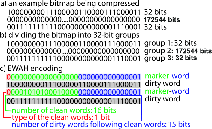
Current microprocessors perform operations over words of 32 or 64 bits and not individual bits. Hence, the CPU cost of RLE might be large [24]. By trading some compression for more speed, Antoshenkov [5] defined a RLE variant working over bytes instead of bits (BBC). Trading even more compression for even more speed, Wu et al. [3] proposed WAH. Their scheme is made of two different types of words. The first bit of every word is true (1) for a running sequence of 31-bit clean words (0x00 or 1x11), and false (0) for a verbatim (or dirty) 31-bit word. Running sequences are stored using 1 bit to distinguish between the type of word (0 for 0x00 and 1 for 1x11) and 30 bits to represent the number of consecutive clean words. Hence, a bitmap of length 62 containing a single 1-bit at position $32$ would be coded as the words 100x01 and 010x00. Because dirty words are stored in units of 31 bits using 32 bits, WAH compression can expand the data by 3%. We studied a WAH variant that we called Enhanced Word-Aligned Hybrid (EWAH): in a technical report, Wu et al. [25] called the same scheme Word-Aligned Bitmap Code (WBC). Contrary to WAH compression, EWAH may never (within 0.1%) generate a compressed bitmap larger than the uncompressed bitmap. It also uses only two types of words (see Fig. 1), where the first type is a 32-bit verbatim word. The second type of word is a marker word: the first bit indicates which clean word will follow, half the bits (16 bits) are used to store the number of clean words, and the rest of the bits (15 bits) are used to store the number of dirty words following the clean words. EWAH bitmaps begin with a marker word.

3.1 Comparing WAH and EWAH

Because EWAH uses only 16 bits to store the number of clean words, it may be less efficient than WAH when there are many consecutive sequences of $2^{16}$ identical clean words. The seriousness of this problem is limited because tables are indexed in blocks of rows which fit in RAM: the length of runs does not grow without bounds even if the table does. In § 7.3, we show that this overhead on compressing clean words is at most 14% on our sorted data sets—and this percentage is much lower (3%) when considering only unsorted tables. Furthermore, about half of the compressed bitmaps are made of dirty words, on which EWAH is 3% more efficient than WAH.

We can alleviate this compression overhead over clean words in several ways. On the one hand, we can allocate more than half of the bits to encode the runs of clean words [25]. On the other hand, when a marker word indicates a run of $2^{16}$ clean words, we could use the convention that the next word indicates the number of remaining clean words. Finally, this compression penalty is less relevant when using 64-bit words instead of 32-bit words.

When there are long runs of dirty words in some of the bitmaps, EWAH might be preferable—it will access each dirty word at most once, whereas a WAH decoder checks the first bit of each dirty word to ascertain it is a dirty word. An EWAH decoder can skip a sequence of dirty words whereas a WAH decoder must access them all. For example, if we compute a logical AND between a bitmap containing only dirty words, and another containing very few non-zero words, the running time of the operation with EWAH compression will only depend on the small compressed size of the second bitmap.

Figure 1: Enhanced Word-Aligned Hybrid (EWAH)

3.2 Constructing a bitmap index

Given $L$ bitmaps and a table having $n$ rows and $c$ columns, we can naïvely construct a bitmap index in time $O(nL)$ by appending a word to each compressed bitmap every 32 or 64 rows. We found this approach impractically slow when $L$ was large—typically, with $k=1$. Instead, we construct bitmap indexes in time proportional to the size of the index (see Algorithm 1): within each block of $w$ rows (e.g., $w=32$), we store the values of the bitmaps in a set—omitting any unsolicited bitmap, whose values are all false (0x00). We use the fact we can add several clean words of the same type to a compressed bitmap in constant time.

Our implementation is able to generate the index efficiently on disk, even with extremely large tables and millions of (possibly small) compressed bitmaps, using horizontal partitioning: we divide the table’s rows into large blocks, such that each block’s compressed index fits in a fixed memory budget (256 MiB). Each block of bitmaps is written sequentially [26] and preceded by an array of 4-byte integers containing the location of each bitmap within the block.

  Construct: $B_{1},\ldots,B_{L}$, $L$ compressed bitmaps

  $\mathrm{length}(B_{i})$ is current (uncompressed) length (in bits) of bitmap $B_{i}$

  $w$ is word length in bits, a power of 2 (e.g., $w=32$)

  $\omega_{i}\leftarrow 0$ for $1\leq i\leq L$.

  $c\leftarrow 1$ {row counter}

  $\mathcal{N}\leftarrow\emptyset$ {$\mathcal{N}$ records the dirtied bitmaps}

  for each table row do

     for each attribute in the row do

        for each bitmap $i$ corresponding to the attribute value do

           set to true the $(c\bmod w)^{\mathrm{th}}$ bit of word $\omega_{i}$

           $\mathcal{N}\leftarrow\mathcal{N}\cup\{i\}$

     if $c$ is a multiple of $w$ then

        for $i$ in $\mathcal{N}$ do

           add $c/w-\mathrm{length}(B_{i})-1$ clean words (0x00) to $B_{i}$

           add the word $\omega_{i}$ to bitmap $B_{i}$

           $\omega_{i}\leftarrow 0$

        $\mathcal{N}\leftarrow\emptyset$

     $c\leftarrow c+1$

  for $i$ in {1,2,…,L} do

     add $c/w-|B_{i}|-1$ clean words (0x00) to $B_{i}$

Algorithm 1 Constructing bitmaps. For simplicity, we assume the number of rows is a multiple of the word size.

3.3 Faster operations over compressed bitmaps

Beside compression, there is another reason to use RLE: it makes operations faster [3]. Given (potentially many) compressed bitmaps $B_{1},\ldots,B_{L}$ of sizes $|B_{i}|$, Algorithm 2 computes $\land_{i=1}^{L}B_{i}$ and $\lor_{i=1}^{L}B_{i}$ in time $O(L\sum_{i}|B_{i}|)$. For BBC, WAH, EWAH and all similar RLE variants, similar algorithms exists: we only present the results for traditional RLE to simplify the exposition.

Indeed, within a given pass through the main loop of Algorithm 2, we need to compute the minimum and the maximum between $L$ $w$-bit counter values which requires $O(L)$ time. Hence, the running time is determined by the number of iterations, which is bounded by the sum of the compressed sizes of the bitmaps ($\sum_{i}|B_{i}|$).

For RLE with variable-length counters, the runs are encoded using $\log n$ bits and so each pass through the main loop of Algorithm 2 will be in $O(L\log n)$, and a weaker result is true: the computation is in time $O(L\sum_{i}|B_{i}|\log n)$. We should avoid concluding that the complexity is worse due to the $\log n$ factor: variable-length RLE can generate smaller bitmaps than fixed-length RLE.

  INPUT: $L$ bitmaps $B_{1},\ldots B_{L}$

  $I_{i}\leftarrow$ iterator over the runs of identical bits of $B_{i}$

  $\Gamma\leftarrow$ representing the aggregate of $B_{1},\ldots B_{L}$ (initially empty)

  while some iterator has not reached the end do

     let $a^{\prime}$ be the maximum of all starting values for the runs of $I_{1},\ldots,I_{L}$

     let $a$ be the minimum of all ending values for the runs of $I_{1},\ldots,I_{L}$

     append run $[a^{\prime},a]$ to $\Gamma$ with value determined by $\gamma(I_{1},\ldots,I_{L})$

     increment all iterators whose current run ends at $a$.

Algorithm 2 Generic $O(L\sum_{i}|B_{i}|)$ algorithm to compute any bitwise operations between $L$ bitmaps. We assume the $L$-ary bitwise operation, $\gamma$, itself is in $O(L)$.

A stronger result is possible if the bitwise operation is updatable in $O(\log L)$ time. That is, given the result of an updatable $L$-ary operation $\gamma(b_{1},b_{2},\ldots,b_{L})$, we can compute the updated value when a single bit is modified ($b^{\prime}_{i}$),

$$\gamma(b_{1},b_{2},\ldots,b_{i-1},b^{\prime}_{i},b_{i+1},\ldots,b_{L}),$$

in $O(\log L)$ time. All symmetric Boolean functions are so updatable: we merely maintain a count of the number of ones, which (for a symmetric function) determines its value. Symmetric functions include AND, OR, NAND, NOR, XOR and so forth. For example, given the number of 1-bits in a set of $L$ bits, we can update their logical AND or logical OR aggregation ( $\land_{i=1}^{L}b_{i}$, $\lor_{i=1}^{L}b_{i}$) in constant time given that one of the bits changes its value. Fast updates also exist for functions that are symmetric except that specified inputs are inverted (e.g., Horn clauses).

From Algorithm 3, we have the following lemma. (The result is presented for fixed-length counters; when using variable-length counters, multiply the complexity by $\log n$.)

Lemma 2

Given $L$ RLE-compressed bitmaps of sizes $|B_{1}|,|B_{2}|,\ldots,|B_{L}|$ and any bitwise logical operation computable in $O(L)$ time, the aggregation of the bitmaps is in time $O(\sum_{i=1}^{L}|B_{i}|L)$. If the bitwise operation is updatable in $O(\log L)$ time, the aggregation is in time $O(\sum_{i=1}^{L}|B_{i}|\log L)$.

  INPUT: $L$ bitmaps $B_{1},\ldots B_{L}$

  $I_{i}\leftarrow$ iterator over the runs of identical bits of $B_{i}$

  $\Gamma\leftarrow$ representing the aggregate of $B_{1},\ldots B_{L}$ (initially empty)

  $\gamma$ be the bit value determined by $\gamma(I_{i},\ldots,I_{L})$

  $H^{\prime}$ is an $L$-element max-heap storing starting values of the runs (one per bitmap)

  $H$ is an $L$-element min-heap storing ending values of the runs and an indicator of which bitmap

  a table $T$ mapping each bitmap to its entry in $H^{\prime}$

  while some iterator has not reached the end do

     let $a^{\prime}$ be the maximum of all starting values for the runs of $I_{1},\ldots,I_{L}$, determined from $H^{\prime}$

     let $a$ be the minimum of all ending values for the runs of $I_{1},\ldots,I_{L}$, determined from $H$

     append run $[a^{\prime},a]$ to $\Gamma$ with value $\gamma$

     for iterator $I_{i}$ with a run ending at $a$ (selected from $H$) do

        increment $I_{i}$ while updating $\gamma$ in $O(\log L)$ time

        pop $a$ value from $H$, insert new ending run value to $H$

        from hash table, find old starting value in $H^{\prime}$, and increase it to the new starting value

Algorithm 3 Generic $O(\sum_{i}|B_{i}|\log L)$ algorithm to compute any bitwise operations between $L$ bitmaps updatable in $O(\log L)$ time.

Corollary 1

This result is also true for word-aligned (BBC, WAH or EWAH) compression.

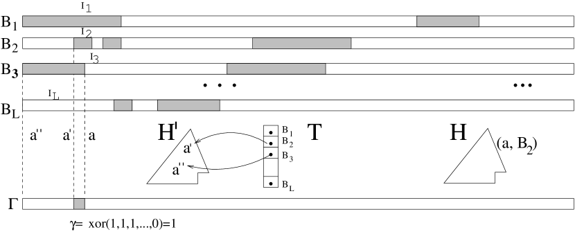
See Fig. 2, where we show the XOR of $L$ bitmaps. This situation depicted has just had $I_{2}$ incremented, and $\gamma$ is about to be updated to reflect the change of $B_{2}$ from ones to zeros. The value of $a$ will then be popped from $H$, whose minimum value will then be the end of the $I_{1}$ run. Table $T$ will then allow us to find and increase the key of $B_{2}$’s entry in $H^{\prime}$, where it will become $a+1$ and likely be promoted toward the top of $H^{\prime}$.

Figure 2: Algorithm 3 in action.

In the rest of this section, we assume an RLE encoding such that the merger of two running lengths reduces the total size (0 repeated $x$ times and 0 repeated $y$ times, becomes 0 repeated $x+y$ times). These encodings include BBC, WAH and EWAH. We also consider only fixed-length counters; for variable-length counters, the running time complexity should have the bitmap index size multiplied by $\log n$.

From Algorithm 3, we have that $|\land_{i\in S}B_{i}|\leq|\sum_{i\in S}B_{i}|$, $|\lor_{i\in S}B_{i}|\leq|\sum_{i\in S}B_{i}|$, and so on for other binary bitwise operation such as $\oplus$. This bound is practically optimal: e.g., the logical AND of the bitmaps 10…10 ($n$ runs) and 11…11 (1 run) is 10…10 ($n$ runs).

Hence, for example, when computing $B_{1}\land B_{2}\land B_{3}\land+\cdots\land B_{L}$ we may start with the computation of $B_{1}\land B_{2}=B_{1,2}$ in $O(|B1|+|B2|)$ time. The bitmap $B_{1,2}$ is of size at most $|B_{1}|+|B_{2}|$, hence $B_{1,2}\land B_{3}$ can be done in time $O(|B_{1}|+|B_{2}|+|B_{3}|)$. Hence, the total running time is in $O(\sum_{i=1}^{L}(L-i+1)|B_{i}|)$.

Hence, there are at least three different generic algorithms to aggregate a set of $L$ bitmaps for these most common bitwise operations:

• We use Algorithm 3, which runs in time $O((\sum_{i=1}^{L}|B_{i}|)\log L)$. It generates a single output bitmap, but it uses two L-element heaps. It works for a wide range of queries, not only simple queries such as $\lor_{i=1}^{L}B_{i}$.

• We aggregate two bitmaps at a time starting with $B_{1}$ and $B_{2}$, then aggregating the result with $B_{3}$, and so on. This requires time $O(\sum_{i=1}^{L}(L-i+1)|B_{i}|)$. While only a single temporary compressed bitmap is held in memory, $L-1$ temporary bitmaps are created. To minimize processing time, the input bitmaps can be sorted in increasing size.

• We can store the bitmaps in a priority queue [27]. We repeatedly pop the two smallest bitmaps, and insert the aggregate of the two bitmaps. This approach runs in time $O((\sum_{i=1}^{L}|B_{i}|)\log L)$, and it generates $L-1$ intermediate bitmaps.

• Another approach is to use in-place computation [27]: (1) an uncompressed bitmap is created in time $O(n)$ (2) we aggregate the uncompressed bitmap with the each one of the compressed bitmaps (3) the row IDs are extracted from the uncompressed bitmap in time $O(n)$. For logical OR (resp. AND) aggregates, the uncompressed bitmap is initialized with zeroes (resp. ones). The total cost is in $O(Ln)$: $L$ passes over the uncompressed bitmap will be required. However, when processing each compressed bitmap, we can skip over portions of the uncompressed bitmaps e.g., when we compute a logical OR, we can omit runs of zeroes. If the table has been horizontally partitioned, it will be possible to place the uncompressed bitmap in main memory.

We can minimize the complexity by choosing the algorithm after loading the bitmaps. For example, to compute logical OR over many bitmaps with long runs of zeroes—or logical AND over many bitmaps with long runs of ones—an in-place computation might be preferable. When there are few bitmaps, computing the operation two bitmaps at a time is probably efficient. Otherwise, using Algorithm 3 or a priority queue [27] might be advantageous. Unlike the alternatives, Algorithm 3 is not limited to simple queries such as $\lor_{i=1}^{L}B_{i}$.

4 Finding the best reordering is NP-Hard

Let $d(r,s)$ be the number of bits differing between rows $r$ and $s$. Our problem is to find the best ordering of the rows $r_{i}$ so as to minimize $\sum_{i}d(r_{i},r_{i+1})$. Pinar et al. have reduced the row-reordering problem to the Traveling Salesman Problem (TSP) [9, Theorem 1] using $d$ as the distance measure. Because $d$ satisfies the triangle inequality, the row-reordering problem can be approximated with 1.5-optimal cubic-time algorithms [28]. Pinar and Heath [29] proved that the row-reordering problem is NP-Hard by reduction from the Hamiltonian path problem.

However, the hardness of the problem depends on $L$ being variable. If the number $L$ of bitmaps were a constant, the next lemma shows that the problem would not be NP-hard: an (impractical) linear-time solution is possible.

Lemma 3

For any constant number of bitmaps $L$, the row-reordering problem requires only $O(n)$ time.

Proof 2

Suppose that an optimal row ordering is such that identical rows do not appear consecutively. Pick any row value—any sequence of $L$ bits appearing in the bitmap index—and call it $a$. Consider two occurrences of $a$, where one occurrence of the row value $a$ appears between the row values $b$ and $c$: we may have $b=a$ and/or $c=a$. Because the Hamming distance satisfies the triangle inequality, we have $d(b,c)\geq d(b,a)+d(a,c)$. Hence, we can move the occurrence of $a$ from between $b$ and $c$, placing it instead with any other occurrence of $a$—without increasing total cost, $\sum_{i}d(r_{i},r_{i+1})$. Therefore, there is an optimal solution with all identical rows clustered.

In a bitmap index with $L$ bitmaps, there are only $2^{L}$ different possible distinct rows, irrespective of the total number of rows $n$. Hence, there are at most $(2^{L})!$ solutions to enumerate where all identical rows are clustered, which concludes the proof.

If we generalize the row-reordering problem to the word-aligned case, the problem is still NP-hard. We can formalize the problem as such: order the rows in a bitmap index such that the storage cost of any sequence of identical clean words (0x00 or 1x11) costs $w$ bits whereas the cost of any other word is $w$ bits.

Theorem 1

The word-aligned row-reordering problem is NP-hard if the number of bits per word ($w$) is a constant.

Proof 3

Consider the case where each row of the bitmap is repeated $w$ times. It is possible to reorder these identical rows so that they form only clean words (1x11 and 0x00). There exists an optimal solution to the word-aligned row-reordering problem obtained by reordering these blocks of $w$ identical rows. The problem of reordering these clean words is equivalent to the row-ordering problem, which is known to be NP-hard.

5 Sorting to improve compression

Sorting can benefit bitmap indexes at several levels. We can sort the rows of the table. The sorting order depends itself on the order of the table columns. And finally, we can allocate the bitmaps to the attribute values in sorted order.

5.1 Sorting rows

Reordering the rows of a compressed bitmap index can improve compression. Whether using RLE, BBC, WAH or EWAH, the problem is NP-hard (see § 4). A simple heuristic begins with an uncompressed index. Rows (binary vectors) are then rearranged to promote runs. In the process, we may also reorder the bitmaps. This is the approach of Pinar et al. [9], Sharma and Goyal [7], Canahuate et al. [10], and Apaydin et al. [8], but it uses $\Omega(nL)$ time. For the large dimensions and number of rows we have considered, it is infeasible. A more practical approach is to reorder the table, then construct the compressed index directly (see § 5.2.2); we can also reorder the table columns prior to sorting (see § 5.3).

Sorting lexicographically large files in external memory is not excessively expensive [30, 31]. With a memory buffer of $M$ elements, we can sort almost $M^{2}$ elements in two passes.

Several types of ordering can be used for ordering rows.

• In lexicographic order, a sequence $a_{1},a_{2},\ldots$ is smaller than another sequence $b_{1},b_{2},\ldots$ if and only if there is a $j$ such that $a_{j}<b_{j}$ and $a_{i}=b_{i}$ for $i<j$. The Unix sort command provides an efficient means of sorting flat files into lexicographic order; in under 10 s our test computer (see § 7) sorted a 5-million-line, 120 MB file. SQL supports lexicographic sort via ORDER BY.

• We may cluster runs of identical rows. This problem can be solved with hashing algorithms, by multiset discrimination algorithms [32], or by a lexicographic sort. While sorting requires $\Omega(n\log n)$ time, clustering identical facts requires only linear time ($O(n)$). However, the relative efficiency of clustering decreases drastically with the number of dimensions. The reason is best illustrated with an example. Consider lexicographically-sorted tuples $(a,a)$, $(a,b)$, $(b,c)$, $(b,d)$. Even though all these tuples are distinct, the lexicographical order is beneficial to the first dimension. Random multidimensional row clustering fails to cluster the values within columns.

• Instead of fully ordering all of the rows, we may reorder rows only within disjoint blocks (see § 7.4). Block-wise sorting is not competitive.

• Gray-code (GC) sorting, examined next.

GC sorting is defined over bit vectors [9]. The list of 2-of-4 codes in increasing order is 0011, 0110, 0101, 1100, 1010, 1001. Intuitively, the further right the first bit is, the smaller the code is, just as in the lexicographic order. However, contrary to the lexicographic order, the further left the second bit is, the smaller the code is. Similarly, for a smaller code, the third bit should be further right, the fourth bit should be further left and so on. Formally, we define the Gray-code order as follows.

Definition 1

The sequence $a_{1},a_{2},\ldots$ is smaller than $b_{1},b_{2},\ldots$ if and only if there exists $j$ such that $a_{j}=a_{1}\oplus a_{2}\oplus\ldots\oplus a_{j-1}$, $b_{j}\not=a_{j}$, and $a_{i}=b_{i}$ for $i<j$.

We denote this ordering by $<_{\mathrm{gc}}$, as opposed to the normal lexicographic ordering, $<_{\mathrm{lex}}$. The reflexive versions of these are $\leq_{\mathrm{gc}}$ and $\leq_{\mathrm{lex}}$, respectively.

Algorithm 4, an adaptation of Ernvall’s procedure [33, 34] to sparse data, shows how to compare sparse GC bit vectors $v_{1}$ and $v_{2}$ in time $O(\min(|v_{1}|,|v_{2}|)$ where $|v_{i}|$ is the number of true value in bit vector $v_{i}$. Sorting the rows of a bitmap index without materializing the uncompressed bitmap index is possible: we implemented an $O(nck\log n)$-time solution for $k$-of-$N$ indexes using an external-memory B-tree [35] ($c$ is the number of columns). As values, we used the rows of the table, and as keys, we used the position of the ones in the bitmap row as 32-bit integers—some of our indexes have half a million bitmaps. Hence, we used $4ck$ bytes per row for storing the keys alone. Both keys and values were compressed using LZ77 to minimize I/O costs—compression improved performance noticeably in our informal tests. We expected that this implementation would be significantly slower than lexicographic sorting, but the degree of difference surprised us: our implementation proved to be two orders of magnitude slower than lexicographic sort using the Unix sort command.

For some of our tests (see § 7.9), we wish to rearrange the order of the bitmaps prior to GC sorting. We get this result by applying the appropriate permutation to the positions that form the B-tree keys, during the B-tree’s construction.

  INPUT: arrays $a$ and $b$ representing the position of the ones in two bit vectors, $a^{\prime}$ and $b^{\prime}$

  OUTPUT: whether $a^{\prime}<_{\mathrm{gc}}b^{\prime}$

  $f\leftarrow\texttt{true}$

  $m\leftarrow\min(\textrm{length}(a),\textrm{length}(b))$

  for $p$ in $1,2,\ldots,m$ do

     return $f$ if $a_{p}>b_{p}$ and $\lnot f$ if $a_{p}<b_{p}$

     $f\leftarrow\lnot f$

  return $\lnot f$ if $\textrm{length}(a)>\textrm{length}(b)$, $f$ if $\textrm{length}(b)>\textrm{length}(a)$, and false otherwise

Algorithm 4 Gray-code less comparator between sparse bit vectors

For RLE, the best ordering of the rows of a bitmap index minimizes the sum of the Hamming distances: $\sum_{i}h(r_{i},r_{i+1})$ where $r_{i}$ is the $i^{\mathrm{th}}$ row, for $h(x,y)=\left|\rule{0.0pt}{9.49997pt}\{i|x_{i}\not=y_{i}\}\right|$. If all $2^{L}$ different rows are present, the GC sort would be an optimal solution to this problem [9]. The following proposition shows that GC sort is also optimal if all ${N\choose k}$ $k$-of-$N$ codes are present. The same is false of lexicographic order when $k>1$: 0110 immediately follows 1001 among 2-of-4 codes, but their Hamming distance is 4.

Proposition 1

We can enumerate, in GC order, all $k$-of-$N$ codes in time $O(k{N\choose k})$ (optimal complexity). Moreover, the Hamming distance between successive codes is minimal (=2).

Proof 4

Let $a$ be an array of size $k$ indicating the positions of the ones in $k$-of-$N$ codes. As the external loop, vary the value $a_{1}$ from 1 to $N-k+1$. Within this loop, vary the value $a_{2}$ from $N-k+2$ down to $a_{1}+1$. Inside this second loop, vary the value of $a_{3}$ from $a_{2}+1$ up to $N-k+3$, and so on. By inspection, we see that all possible codes are generated in decreasing GC order. To see that the Hamming distance between successive codes is 2, consider what happens when $a_{i}$ completes a loop. Suppose that $i$ is odd and greater than 1, then $a_{i}$ had value $N-k+i$ and it will take value $a_{i-1}+1$. Meanwhile, by construction, $a_{i+1}$ (if it exists) remains at value $N-k+i+1$ whereas $a_{i+2}$ remains at value $N-k+i+2$ and so on. The argument is similar if $i$ is even.

For encodings like BBC, WAH or EWAH, GC sorting is suboptimal, even when all $k$-of-$N$ codes are present. For example consider the sequence of rows 1001, 1010, 1100, 0101, 0101, 0110, 0110, 0011. Using 4-bit words, we see that a single bitmap contains a clean word (0000) whereas by exchanging the fifth and second row, we get two clean words (0000 and 1111).

5.2 Sorting bitmap codes

For a simple index, the map from attribute values to bitmaps is inconsequential; for $k$-of-$N$ encodings, some bitmap allocations are more compressible: consider an attribute with two overwhelmingly frequent values and many other values that occur once each. If the table rows are given in random order, the two frequent values should have codes that differ in Hamming distance as little as possible to maximize compression (see Fig. 3 for an example). However, it is also important to allocate bitmaps well when the table is sorted, rather than randomly ordered.

1	0	0	1
0	1	1	0
1	0	0	1
0	1	1	0
0	1	1	0
1	0	0	1

1	0	0	1
1	1	0	0
1	0	0	1
1	1	0	0
1	1	0	0
1	0	0	1

Figure 3: Two bitmaps representing the sequence of values a,b,a,b,b,a using different codes. If codes have a Hamming distance of two (right), the result is more compressible than if the Hamming distance is four (left).

There are several ways to allocate the bitmaps. Firstly, the attribute values can be visited in alphabetical or numerical order, or—for histogram-aware schemes—in order of frequency. Secondly, the bitmap codes can be used in different orders. We consider lexicographical ordering (1100, 1010, 1001, 0110, …) and GC order (1001, 1010, 1100, 0101, …) ordering (see proof of Proposition 1).

Binary-Lex denotes sorting the table lexicographically and allocating bitmap codes so that the $i^{\mathrm{th}}$ attribute gets the $i^{\mathrm{th}}$ numerically smallest bitmap code, when codes are viewed as binary numbers. Gray-Lex is similar, except that the $i^{\mathrm{th}}$ attribute gets the rank-$i$ bitmap code in GC order. (Binary-Lex and Gray-Lex coincide when $k=1$.) These two approaches are histogram oblivious—they ignore the frequencies of attribute values.

Knowing the frequency of each attribute value can improve code assignment when $k>1$. Within a column, Binary-Lex and Gray-Lex order runs of identical values irrespective of the frequency: the sequence afcccadeaceabe may become aaaabccccdeeef. For better compression, we should order the attribute values—within a column—by their frequency (e.g., aaaacccceeebdf). Allocating the bitmap codes in GC order to the frequency-sorted attribute values, our Gray-Frequency sorts the table rows as follows. Let $f(a_{i})$ be the frequency of attribute $a_{i}$. Instead of sorting the table rows $a_{1},a_{2},\ldots,a_{d}$, we lexicographically sort the extended rows $f(a_{1}),a_{1},f(a_{2}),a_{2},\ldots,f(a_{d}),a_{d}$ (comparing the frequencies numerically.) The frequencies $f(a_{i})$ are discarded prior to indexing.

5.2.1 No optimal ordering when $k>1$

No allocation scheme is optimal for all tables, even if we consider only lexicographically sorted tables.

Proposition 2

For any allocation $\mathcal{C}$ of attribute values to $k$-of-$N$ codes, there is a table where $\mathcal{C}$ leads to a suboptimal index.

Proof 5

Consider a lexicographically sorted table, where we encode the second column with $\mathcal{C}$. We construct a table where $\mathcal{C}$ is worse than some other ordering $\mathcal{C}^{\prime}$. The first column of the table is for attribute $A_{1}$, which is the primary sort key, and the second column is for attribute $A_{2}$. Choose any two attribute values $v_{1}$ and $v_{2}$ from $A_{2}$, where $\mathcal{C}$ assigns codes of maximum Hamming distance (say $d$) from one another. If $A_{2}$ is large enough, $d>2$. Our bad input table has unique ascending values in the first column, and the second column alternates between $v_{1}$ and $v_{2}$. Let this continue for $w$ rows. On this input, there will be $d$ bitmaps that are entirely dirty for the second column. Other bitmaps in the second column are made entirely of identical clean words.

Now consider $\mathcal{C}^{\prime}$, some allocation that assigns $v_{1}$ and $v_{2}$ codewords at Hamming distance 2. On this input, $\mathcal{C^{\prime}}$ produces only 2 dirty words in the bitmaps for $A_{2}$. This is fewer dirty words than $\mathcal{C}$ produced.

Because bitmaps containing only identical clean words use less storage than bitmaps made entirely of dirty words, we have that allocation $\mathcal{C}^{\prime}$ will compress the second column better. This concludes the proof.

5.2.2 Gray-Lex allocation and GC-ordered indexes

Despite the pessimistic result of Proposition 2, we can focus in choosing good allocations for special cases, such as dense indexes (including those where most of the possible rows appear), or for typical sets of data.

For dense indexes, GC sorting is better [9] at minimizing the number of runs, a helpful effect even with word-aligned schemes. However, as we already pointed out, the approach used by Pinar et al. [9] requires $\Omega(nL)$ time. For technical reasons, even our more economical B-tree approach is much slower than lexicographic sorting. As an alternative, we propose a low-cost way to GC sort $k$-of-$N$ indexes, using only lexicographic sorting and Gray-Lex allocation.

We now examine Gray-Lex allocation more carefully, to prove that its results are equivalent to building the uncompressed index, GC sorting, and then compressing the index.

Let $\gamma_{i}$ be the invertible mapping from attribute $i$ to the $k_{i}$-of-$N_{i}$ code—written as an $N_{i}$-bit vector. Gray-Lex implies a form of monotonicity: for $a$ and $a^{\prime}$ belonging to the $i^{\mathrm{th}}$ attribute, $A_{i}$, $a\leq a^{\prime}\Rightarrow\gamma_{i}(a)\leq_{\mathrm{gc}}\gamma_{i}(a^{\prime})$. The overall encoding of a table row $r=(a_{1},a_{2},\ldots,a_{c})$ is obtained by applying each $\gamma_{i}$ to $a_{i}$, and concatenating the $c$ results. I.e., $r$ is encoded into

$$\Gamma(r)=(\overbrace{\alpha_{1},\alpha_{2},\ldots\alpha_{N_{1}}}^{\gamma_{1}(a_{1})},\overbrace{\alpha_{N_{1}+1},\ldots\alpha_{N_{1}+N_{2}}}^{\gamma_{2}(a_{2})},\ldots\overbrace{\alpha_{L-N_{c}+1},\ldots\alpha_{L}}^{\gamma_{c}(a_{c})})$$

where $\alpha_{i}\in\{0,1\}$ for all $i$.

First, let us assume that we use only $k$-of-$N$ codes, for $k$ even. Then, the following proposition holds.

Proposition 3

Given two table rows $r$ and $r^{\prime}$, using Gray-Lex $k$-of-$N$ codes for $k$ even, we have $r\leq_{\mathrm{lex}}r^{\prime}\iff\Gamma(r)\leq_{\mathrm{gc}}\Gamma(r^{\prime})$. The values of $k$ and $N$ can vary from column to column.

Proof 6

We write $r=(a_{1},\ldots,a_{c})$ and $r^{\prime}=(a^{\prime}_{1},\ldots,a^{\prime}_{c})$. We note $(\alpha_{1},\ldots,\alpha_{L})=\Gamma(r)$ and $(\alpha^{\prime}_{1},\ldots,\alpha^{\prime}_{L})=\Gamma(r^{\prime})$. Without loss of generality, we assume $\Gamma(r)\leq_{\mathrm{gc}}\Gamma(r^{\prime})$. First, if $\Gamma(r)=\Gamma(r^{\prime})$, then $r=r^{\prime}$ since each $\gamma_{i}$ is invertible.

We now proceed to the case where $\Gamma(r)<_{\mathrm{gc}}\Gamma(r^{\prime})$. Since they are not equal, Definition 1 implies there is a bit position $t$ where they first differ; at position $t$, we have that $\alpha_{t}=\alpha_{1}\oplus\alpha_{2}\oplus\cdots\oplus\alpha_{t-1}$. Let $\hat{t}$ denote the index of the attribute associated with bitmap $t$. In other words, $N_{1}+N_{2}+\cdots+N_{\hat{t}-1}<t\leq N_{1}+N_{2}+\cdots+N_{\hat{t}}$. Let $t^{\prime}$ be the first bitmap of the block for attribute $\hat{t}$; i.e., $t^{\prime}=N_{1}+N_{2}+\cdots+N_{\hat{t}-1}+1$.

$$\begin{array}[]{rll}\Gamma(r)<_{\mathrm{gc}}&\Gamma(r^{\prime})&\\ \iff&\alpha_{t}=\bigoplus_{i=1}^{t-1}\alpha_{i}\ \wedge\ \alpha_{t}\not=\alpha^{\prime}_{t}\ \wedge\ \bigwedge_{i=1}^{t-1}(\alpha_{i}=\alpha^{\prime}_{i})&\mbox{Def.~{}\ref{GCordering}}\\ \iff&\alpha_{t}=\bigoplus_{i=1}^{t^{\prime}-1}\alpha_{i}\oplus\bigoplus_{i=t^{\prime}}^{t-1}\alpha_{i}\ \wedge\ \alpha_{t}\not=\alpha^{\prime}_{t}&\\ &\wedge\ \bigwedge_{i=1}^{t^{\prime}-1}(\alpha_{i}=\alpha^{\prime}_{i})\ \wedge\ \bigwedge_{i=t^{\prime}}^{t-1}(\alpha_{i}=\alpha^{\prime}_{i})&\mbox{associativity}\\ \iff&\alpha_{t}=0\oplus\bigoplus_{i=t^{\prime}}^{t-1}\alpha_{i}\ \wedge\ \alpha_{t}\not=\alpha^{\prime}_{t}&\mbox{all codes are $k$-of-$N$}\\ &\wedge\ \bigwedge_{i=1}^{t^{\prime}-1}(\alpha_{i}=\alpha^{\prime}_{i})\ \wedge\ \bigwedge_{i=t^{\prime}}^{t-1}(\alpha_{i}=\alpha^{\prime}_{i})&\mbox{and $k$ is even}\\ \iff&\alpha_{t}=\bigoplus_{i=t^{\prime}}^{t-1}\alpha_{i}\ \wedge\ \alpha_{t}\not=\alpha^{\prime}_{t}&\\ &\wedge\ \bigwedge_{i=1}^{\hat{t}-1}(a_{i}=a^{\prime}_{i})\ \wedge\ \bigwedge_{i=t^{\prime}}^{t-1}(\alpha_{i}=\alpha^{\prime}_{i})&\mbox{$\gamma_{i}$ is invertible}\\ \iff&\gamma_{\hat{t}}(a_{\hat{t}})<_{\mathrm{gc}}\gamma_{\hat{t}}(a^{\prime}_{\hat{t}})\ \wedge\ \bigwedge_{i=1}^{\hat{t}-1}(a_{i}=a^{\prime}_{i})&\mbox{Def.~{}\ref{GCordering}}\\ \iff&a_{\hat{t}}<_{\mathrm{lex}}a^{\prime}_{\hat{t}}\ \wedge\ \bigwedge_{i=1}^{\hat{t}-1}(a_{i}=a^{\prime}_{i})&\mbox{$\gamma$s are monotone}\\ \iff&r<_{\mathrm{lex}}r^{\prime}&\mbox{Def.\ of lex.\ order}\\ \end{array}$$

$\Box$

If some columns have $k_{i}$-of-$N_{i}$ codes with $k_{i}$ odd, then we have to reverse the order of the Gray-Lex allocation for some columns. Define the alternating Gray-Lex allocation to be such that it has the Gray-Lex monotonicity ($a\leq a^{\prime}\Rightarrow\gamma_{i}(a)\leq_{\mathrm{gc}}\gamma_{i}(a^{\prime})$) when $\sum_{j=1}^{i-1}k_{j}$ is even, and is reversed ($a\leq a^{\prime}\Rightarrow\gamma_{i}(a)\geq_{\mathrm{gc}}\gamma_{i}(a^{\prime})$) otherwise. Then we have the following lemma.

Lemma 4

Given a table to be indexed with alternating Gray-Lex $k$-of-$N$ encoding, the following algorithms have the same output:

• Construct the bitmap index and sort bit vector rows using GC order.

• Sort the table lexicographically and then construct the index.

The values of $k$ and $N$ can vary from column to column.

This result applies to any encoding where there is a fixed number of 1-bits per column. Indeed, in these cases, we are merely using a subset of the $k$-of-$N$ codes. For example, it also works with multi-component encoding where each component is indexed using a unary encoding.

5.2.3 Other Gray codes

In addition to the usual Gray code, many other binary codes have the property that any codeword is at Hamming distance 1 from its successor. Thus, they can be considered “Gray codes” as well, although we shall qualify them to avoid confusion from our standard (“reflected”) Gray code.

Trivially, we could permute columns in the Gray code table, or invert the bit values in particular columns (see Fig. 4). However, there are other codes that cannot be trivially derived from the standard Gray code. Knuth [36, § 7.2.1.1] presents many results for such codes.

0	0	0
0	0	1
0	1	1
0	1	0
1	1	0
1	1	1
1	0	1
1	0	0

(a) 3-bit reflected GC

0	0	0
1	0	0
1	1	0
0	1	0
0	1	1
1	1	1
1	0	1
0	0	1

(b) swap columns 1&3

0	0	1
1	0	1
1	1	1
0	1	1
0	1	0
1	1	0
1	0	0
0	0	0

(c) then invert column 3

Figure 4: The 3-bit reflected GC and two other Gray codes obtained from it, first by exchanging the outermost columns, then by inverting the bits in the third column.

For us, three properties are important:

1. Whether successive $k$-of-$N$ codewords have a Hamming distance of 2.

2. Whether the final codeword is at Hamming distance 1 from the initial codeword. Similarly, whether the initial and final $k$-of-$N$ codewords are at Hamming distance 2.

3. Whether a collection of more than 2 successive codes (or more than 2 successive $k$-of-$N$ codes) has a small expected “collective Hamming distance”. (Count 1 for every bit position where at least two codes disagree. )

The first property is important if we are assigning $k$-of-$N$ codes to attribute values.

The second property distinguishes, in Knuth’s terminology, “Gray paths” from “Gray cycles.” It is important unless an attribute is the primary sort key. E.g., the second column of a sorted table will have its values cycle from the smallest to the largest, again and again.

The third property is related to the “long runs” property [36, 37] of some Gray codes. Ideally, we would want to have long runs of identical values when enumerating all codes. However, for any $L$-bit Gray cycle, every code word terminates precisely one run, hence the number of runs is always $2^{L}$. Therefore, the average run length is always $L$. The distribution of run lengths varies by code, however. When $L$ is large, Goddyn and Grozdjak show there are codes where no run is shorter than $L-3\log_{2}L$; in particular, for $L=1024$, there is a code with no run shorter than 1000 [36, 37]. In our context, this property may be unhelpful: with $k$-of-$N$ encodings, we are interested in only those codewords of Hamming weight $k$. Also, rather than have all runs of approximately length $L$, we might prefer a few very long runs (at the cost of many short ones).

One notable Gray code is constructed by Savage and Winkler [38], henceforth Savage-Winkler (see also Knuth[36, p. 89]). It has all $k$-of-$N$ codes appearing nearly together—interleaved with codes of Hamming weight $k-1$ or $k+1$. Consequently, successive $k$-of-$N$ codes have Hamming distance 2—just like the common/reflected Gray codes.

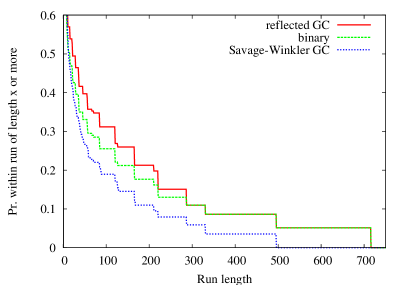
The run-length distributions of the various codes are heavily affected when we limit ourselves to $k$-of-$N$ codes. This is illustrated by Fig. 5, where we examine the run lengths of the 2-of-8 codewords, as ordered by various Gray codes. The code noted as Goddyn-Grozdjak was obtained by inspecting a figure of Knuth [36, Fig. 14d]; some discussion in the exercises may indicate the code is due to Goddyn and Grozdjak [37].

(a) Run-length histogram

(b) Probability within a long run, 2-of-8

(c) Probability within a long run, 3-of-20

(d) Probability within a long run, 4-of-14

Figure 5: Effect of various orderings of the $k$-of-$N$ codes. Top left: Number of runs of length $x$, 2-of-8 codes. For legibility, we omit counts above 30. Goddyn-Grozdjak GC had 42 runs of length 1, binary had 32, and random had 56. Binary, reflected GC and Savage-Winkler had a run of length 15, and reflected GC and binary had a run of length 22. Remainder: Probability that a randomly-chosen bit from an uncompressed index falls in a run of length $x$ or more. Goddyn-Grozdjak and the random ordering were significantly worse and omitted for legibility. In 5(c), when the techniques differed, reflected GC was best, then binary, then Savage-Winkler GC.

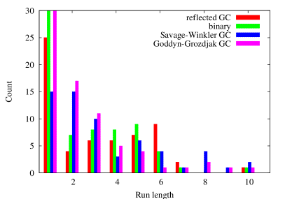
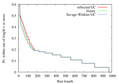
From Fig. 5(a), we see that run-length distributions vary considerably between codes. (These numbers are for lists of $k$-of-$N$ codes without repetition; in an actual table, attribute values are repeated and long runs are more frequent.) Both Goddyn-Grozdjak GC and the random listing stand out as having many short runs. However, the important issue is whether the codes support many sufficiently long runs to get compression benefits.

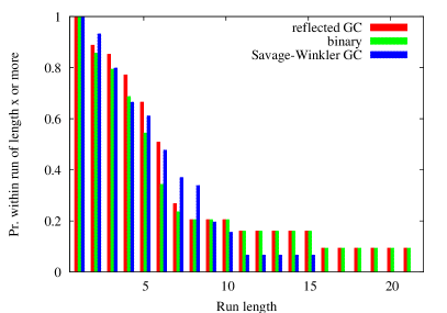
Suppose we list all $k$-of-$N$ codes. Then, we randomly select a single bit position (in one of the $N$ bitmaps). Is there a good chance that this bit position lies within a long run of identical bits? For 2-of-8, 3-of-20 and 4-of-14, we computed these probabilities (see Fig. 5(b), 5(c) and 5(d)). Random ordering and the Goddyn-Grozdjak GC ordering were significantly worse and they have been omitted. From these figure, we see that standard reflected Gray-code ordering is usually best, but ordinary lexicographic ordering is often able to provide long runs. Thus, we might expect that binary allocation will lead to few dirty words when we index a table.

(a) 1000 3-of-20 codes

(b) 1000 4-of-14 codes

Figure 6: Probabilities that a bitmap will contain a dirty word, when several consecutive (how many: $x$-axis) of 1000 possible distinct $k$-of-$N$ codes are found in a 32-row chunk. Effects are shown for values with $k$-of-$N$ codes that are adjacent in reflected GC, Savage-Winkler GC, binary or random order.

Minimizing the number of dirty words

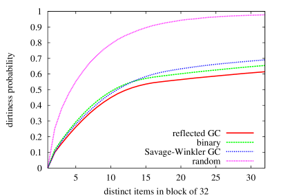
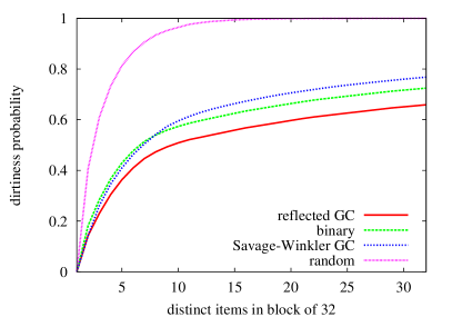
For a given column, suppose that in a block of 32 rows, we have $j$ distinct attribute values. We computed the average number of bitmaps whose word would be dirty (see Fig. 6, where we divide by the number of bitmaps). Comparing $k$-of-$N$ codes that were adjacent in GC ordering against $k$-of-$N$ codes that were lexicographically adjacent, the difference was insignificant for $k=2$. However, GC ordering is substantially better for $k>2$, where bitmaps are denser. The difference between codes becomes more apparent when many attribute values share the same word. Savage-Winkler does poorly, eventually being outperformed even by lexicographic ordering. Selecting the codes randomly is disastrous. Hence, sorting part of a column—even one without long runs of identical values—improves compression for $k>1$.

5.3 Choosing the column order

Lexicographic table sorting uses the $i^{\mathrm{th}}$ column as the $i^{\mathrm{th}}$ sort key: it uses the first column as the main key, the second column to break ties when two rows have the same first component, and so on. Some column orderings may lead to smaller indexes than others.

We model the storage cost of a bitmap index as the sum of the number of dirty words and the number of sequences of identical clean words (1x11 or 0x00). If a set of $L$ bitmaps has $x$ dirty words, then there are at most $L+x$ sequences of clean words; the storage cost is at most $2x+L$. This bound is tighter for sparser bitmaps. Because the simple index of a column has at most $n$ 1-bits, it has at most $n$ dirty words, and thus, the storage cost is at most $3n$. The next proposition shows that the storage cost of a sorted column is bounded by $5n_{i}$.

Proposition 4

Using GC-sorted consecutive $k$-of-$L$ codes, a sorted column with $n_{i}$ distinct values has no more than $2n_{i}$ dirty words, and the storage cost is no more than $4n_{i}+\lceil kn_{i}^{1/k}\rceil$.

Proof 7

Using $\lceil kn_{i}^{1/k}\rceil$ bitmaps is sufficient to represent $n_{i}$ values. Because the column is sorted, we know that the Hamming distance of the bitmap rows corresponding to two successive and different attribute values is 2. Thus every transition creates at most two dirty words. There are $n_{i}$ transitions, and thus at most $2n_{i}$ dirty words. This proves the result.

For $k=1$, Proposition 4 is true irrespective of the order of the values, as long as identical values appear sequentially. Another extreme is to assume that all 1-bits are randomly distributed. Then sparse bitmap indexes have $\approx\delta(r,L,n)=(1-(1-\frac{r}{Ln})^{w})\frac{Ln}{w}$ dirty words where $r$ is the number of 1-bits, $L$ is the number of bitmaps and $w$ is the word length ($w=32$). Hence, we have an approximate storage cost of $2\delta(r,L,n)+\lceil kn_{i}^{1/k}\rceil$. The gain of column $\mathcal{C}$ is the difference between the expected storage cost of a randomly row-shuffled $\mathcal{C}$, minus the storage cost of a sorted $\mathcal{C}$. We estimate the gain by $2\delta(kn,\lceil kn_{i}^{1/k}\rceil,n)-4n_{i}$ (see Fig. 7) for columns with uniform histograms. The gain is modal: it increases until a maximum is reached and then it decreases. The maximum gain is reached at $\approx\left(n(w-1)/2\right)^{k/(k+1)}$: for $n=100,000$ and $w=32$, the maximum is reached at $\approx 1\,200$ for $k=1$ and at $\approx 13\,400$ for $k=2$. Skewed histograms have a lesser gain for a fixed cardinality $n_{i}$.

Figure 7: Storage gain in words for sorting a given column with $100,000$ rows and various number of attribute values ($2\delta(kn,\lceil kn_{i}^{1/k}\rceil,n)-4n_{i}$ ).

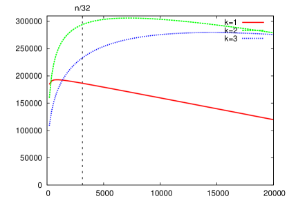
Lexicographic sort divides the $i^{\mathrm{th}}$ column into at most $n_{1}n_{2}\cdots n_{i-1}$ sorted blocks. Hence, it has at most $2n_{1}\cdots n_{i}$ dirty words. When the distributions are skewed, the $i^{\mathrm{th}}$ column will have blocks of different lengths and their ordering depends on how the columns are ordered. For example, if the first dimension is skewed and the second uniform, the short blocks will be clustered, whereas the reverse is true if columns are exchanged. Clustering the short blocks, and thus the dirty words, increases compressibility. Thus, it may be preferable to put skewed columns in the first positions even though they have lesser sorting gain. To assess these effects, we generated data with 4 independent columns: using uniformly distributed dimensions of different sizes (see Fig. 8(a)) and using same-size dimensions of different skew (see Fig. 8(b)). We then determined the Gray-Lex index size—as measured by the sum of bitmap sizes—for each of the 4! different dimension orderings. Based on these results, for sparse indexes ($k=1$), dimensions should be ordered from least to most skewed, and from smallest to largest; whereas the opposite is true for $k>1$.

(a) Uniform histograms with cardinalities 200, 400, 600, 800

(b) Zipfian data with skew parameters 1.6, 1.2, 0.8 and 0.4

Figure 8: Sum of EWAH bitmap sizes in words for various dimension orders on synthetic data ($100,000$ rows). Zipfian columns have 100 distinct values. Ordering “1234” indicates ordering by descending skew (Zipfian) or ascending cardinality (uniform).

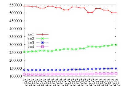
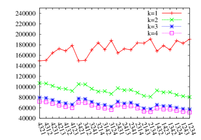
A sensible heuristic might be to sort columns by increasing density ($\approx n_{i}^{-1/k}$). However, a very sparse column ($n_{i}^{1/k}\gg w$) will not benefit from sorting (see Fig. 7) and should be put last. Hence, we use the following heuristic: columns are sorted in decreasing order with respect to $\min(n_{i}^{-1/k},(1-n_{i}^{-1/k})/(4w-1))$: this function is maximum at density $n_{i}^{-1/k}=1/(4w)$ and it goes down to zero as the density goes to 1. In Fig. 8(a), this heuristic makes the best choice for all values of $k$. We consider this heuristic further in § 7.7.

5.4 Avoiding column order

Canahuate et al. [10] propose to permute bitmaps individually prior to sorting, instead of permuting table columns. We compare these two strategies experimentally in § 7.9.

As a practical alternative to lexicographic sort and column (or bitmap) reordering, we introduce Frequent-Component (FC) sorting, which uses histograms to help sort without bias from a fixed dimension ordering. In sorting, we compare the frequency of the $i^{\mathrm{th}}$ most frequent attribute values in each of two rows without regard (except for possible tie-breaking) to which columns they come from. For example, consider the following table:

cat	blue
cat	red
dog	green
cat	green

We have the following (frequency, value) pairs: (1,blue), (1,red), (1,dog), (2,green), and (3,cat). For two rows $r_{1}$ and $r_{2}$, $<_{\mathrm{FC}}$ first compares $(f(a_{1}),a_{1})$ with $(f(a_{2}),a_{2})$, where $a_{1}$ is the least frequent component in $r_{1}$ and $a_{2}$ is the least frequent component in $r_{2}$—$f(a_{i})$ is the frequency of the component $a_{i}$. Values $a_{1}$ and $a_{2}$ can be from different columns. Ties are broken by the second-least-frequent components in $r_{1}$ and $r_{2}$, and so forth. Hence, the sorted table in our example is

dog	green
cat	blue
cat	red
cat	green.

With appropriate pre- and post-processing, it is possible to implement FC using a standard sorting utility such as Unix sort. First, we sort the components of each row of the table into ascending frequency. In this process, each component is replaced by three consecutive components, $f(a)$, $a$, and $\textrm{pos}(a)$. The third component records the column where $a$ was originally found. In our example, the table becomes

(1,dog,1)	(2,green,2)
(1,blue,2)	(3,cat,1)
(1,red,2)	(3,cat,1)
(2,green,2)	(3,cat,1).

Lexicographic sorting (via sort or a similar utility) of rows follows, after which each row is put back to its original value (by removing $f(a)$ and storing $a$ as component $\textrm{pos}(a)$).

6 Picking the right $k$-of-$N$

Choosing $k$ and $N$ are important decisions. We choose a single $k$ value for all dimensions, leaving the possibility of varying $k$ by dimension as future work. Larger values of $k$ typically lead to a smaller index and a faster construction time—although we have observed cases where $k=2$ makes a larger index. However, query times increase with $k$: there is a construction time/speed tradeoff.

6.1 Larger $k$ makes queries slower

We can bound the additional cost of queries. Write ${L_{i}\choose k}=n_{i}$. A given $k$-of-$L_{i}$ bitmap is the result of an OR operation over at most $kn_{i}/L_{i}$ unary bitmaps by the following proposition.

Proposition 5

In $k$-of-$N$ encoding, each attribute value is linked to $k$ bitmaps, and each bitmap is linked to at most $\frac{k}{N}{N\choose k}$ attribute values.

Proof 8

There are ${N\choose k}$ attribute values. Each attribute value is included in $k$ bitmaps. The bipartite graph from attribute values to bitmaps has $k{N\choose k}$ edges. There are $N$ bitmaps, hence $\frac{k}{N}{N\choose k}$ edges per bitmap. This concludes the proof.

Moreover, $n_{i}={L_{i}\choose k}\leq(e\cdot L_{i}/k)^{k}$ by a standard inequality, so that $L_{i}/k\geq n_{i}^{1/k}/e$ or $k/L_{i}\leq e\cdot n_{i}^{-1/k}<3n_{i}^{-1/k}$. Hence, $kn_{i}/L_{i}< 3n_{i}^{(k-1)/k}$.

Because $|\bigvee_{i}B_{i}|\leq\sum_{i}|B_{i}|$, the expected size of such a $k$-of-$L_{i}$ bitmap is no larger than $3n_{i}^{(k-1)/k}$ times the expected size of a unary bitmap. A query looking for one attribute value will have to AND together $k$ of these denser bitmaps. The entire ANDing operation can be done (see the end of § 3) by $k-1$ pairwise ANDs that produce intermediate results whose EWAH sizes are increasingly small: $2k-1$ bitmaps are thus processed. Hence, the expected time complexity of an equality query on a dimension of size $n_{i}$ is no more than $3(2k-1)n_{i}^{\frac{k-1}{k}}$ times higher than the expected cost of the same query on a $k=1$ index. (For $k$ large, we may use see Algorithm 3 to substitute $\log k$ for the $2k-1$ factor.)

For a less pessimistic estimate of this dependence, observe that indexes seldom increase in size when $k$ grows. We may conservatively assume that index size is unchanged when $k$ changes. Therefore, the expected size of one bitmap grows as the reciprocal of the number of bitmaps ($\approx n_{i}^{-1/k}/k$), leading to queries whose cost is proportional to $\approx(2k-1)n_{i}^{-1/k}/k=(2-1/k)n_{i}^{-1/k}$. Relative to the cost for $k=1$, which is proportional to $1/n_{i}$, we can say that increasing $k$ leads to queries that are $(2-1/k)n_{i}^{(k-1)/k}$ times more expensive than on a simple bitmap index.

For example, suppose $n_{i}=100$. Then going from $k=1$ to $k=2$ should increase query cost about 15 fold but no more than 90 fold. In summary, the move from $k=1$ to anything larger can have a dramatic negative effect on query speeds. Once we are at $k=2$, the incremental cost of going to $k=3$ or $k=4$ is low: whereas the ratio $k=2:k=1$ goes as $\sqrt{n_{i}}$, the ratio $k=3:k=2$ goes as $n_{i}^{1/6}$. We investigate this issue experimentally in § 7.10.

6.2 When does a larger $k$ make the index smaller?

Consider the effect of a length 100 run of values $v_{1}$, followed by 100 repetitions of $v_{2}$, then 100 of $v_{3}$, etc. Regardless of $k$, whenever we switch from $v_{1}$ to $v_{i+1}$ at least two bitmaps will have to make transitions between 0 and 1. Thus, unless the transition appears at a word boundary, we create at least 2 dirty words whenever an attribute changes from row to row. The best case, where only 2 dirty words are created, is achieved when $k=1$ for any assignment of bitmap codes to attribute values. For $k>1$ and $N$ as small as possible, it may be impossible to achieve so few dirty words, or it may require a particular assignment of bitmap codes to values.

Encodings with $k>1$ find their use when many (e.g. 15) attribute values fall within a word-length boundary. In that case, a $k=1$ index will have at least 15 bitmaps with transitions (and we can anticipate 15 dirty words). However, if there were only 45 possible values in the dimension, 10 bitmaps would suffice with $k=2$. Hence, there would be at most 10 dirty words and maybe less if we have sorted the data (see Fig. 6).

6.3 Choosing $N$

It seems intuitive, having chosen $k$, to choose $N$ to be as small as possible. Yet, we have observed cases where the resulting 2-of-$N$ indexes are much bigger than 1-of-$N$ indexes. Theoretically, this could be avoided if we allowed larger $N$, because one could aways append an additional 1 to every attribute’s 1-of-$N$ code. Since this would create one more (clean) bitmap than the 1-of-$N$ index has, this 2-of-$N$ index would never be much larger than the 1-of-$N$ index. So, if $N$ is unconstrained, we can see that there is never a significant space advantage to choosing $k$ small.

Nevertheless, the main advantage of $k>1$ is fewer bitmaps. We choose $N$ as small as possible.

7 Experimental results

We present experiments to assess the effects of various factors (choices of $k$, sorting approaches, dimension orderings) in terms of EWAH index sizes. These factors also affect index creation and query times. We report real wall-clock times.

7.1 Platform

Our test programs were written in C++ and compiled by GNU GCC 4.0.2 on an Apple Mac Pro with two double-core Intel Xeon processors (2.66 GHz) and 2 GiB of RAM. Experiments used a 500 GB SATA Hitachi disk (model HDP725050GLA360 [39, 40]), with average seek time (to read) of 14 ms , average rotational latency of 4.2 ms, and capability for sustained transfers at 300 MB/s. This disk also has an on-board cache size of 16 MB, and is formatted for the Mac OS Extended filesystem (journaled). Unless otherwise stated, we use 32-bit binaries. Lexicographic sorts of flat files were done using GNU coreutils sort version 6.9. For constructing all indexes, we used Algorithm 1 because without it, the index creation times were 20–100 times larger, depending on the data set.

7.2 Data sets used

We primarily used four data sets, whose details are summarized in Table 3: Census-Income [41], DBGEN [42], KJV-4grams, and Netflix [43]. DBGEN is a synthetic data set, whereas KJV-4grams is a large list (including duplicates) of 4-tuples of words obtained from the verses in the King James Bible [44], after stemming with the Porter algorithm [45] and removal of stemmed words with three or fewer letters. Occurrence of row $w_{1},w_{2},w_{3},w_{4}$ indicates that the first paragraph of a verse contains words $w_{1}$ through $w_{4}$, in this order. KJV-4grams is motivated by research on Data Warehousing applied to text analysis [46]. Each of column of KJV-4grams contains roughly 8 thousand distinct stemmed words. The Netflix table has 4 dimensions: UserID, MovieID, Date and Rating, having cardinalities 480 189, 17 770, 2 182, and 5. Since the data was originally supplied in 17 700 small files (one file per film), we concatenated them into a flat file with an additional column for the film and randomized the order of its rows using Unix commands such as cat -n file.csv | sort --random-sort | cut -f 2-. All files were initially randomly shuffled.

Table 3: Characteristics of data sets used.

	rows	cols	$\sum_{i}n_{i}$	size
Census-Income	199 523	42	103 419	99.1 MB
4-d projection	199 523	4	102 609	2.96 MB
DBGEN	13 977 980	16	4 411 936	1.5 GB
4-d projection	13 977 980	4	402 544	297 MB
Netflix	100 480 507	4	500 146	2.61 GB
KJV-4grams	877 020 839	4	33 553	21.6 GB

For some of our tests, we chose four dimensions with a wide range of sizes. For Census-Income, we chose age ($d_{1}$), wage per hour ($d_{2}$), dividends from stocks ($d_{3}$) and a numerical value found in the $25^{\mathrm{th}}$ position ($d_{4}$). Their respective cardinalities were 91, 1 240, 1 478 and 99 800. For DBGEN, we selected dimensions of cardinality 7, 11, 2 526 and 400 000. Dimensions are numbered by increasing size: column 1 has fewest distinct values.

7.3 Overview of experiments

Using our test environment, our experiments assessed

• whether a partial (block-wise) sort could save enough time to justify lower quality indexes (§ 7.4);

• the effect that sorting has on index construction time (§ 7.5)

• the merits of various code assignments (§ 7.6);

• whether column ordering (as discussed in § 5.3) has a significant effect on index size (§ 7.7);

• whether the index size grows linearly as the data set grows (§ 7.8);

• whether bitmap reordering is preferable to our column reordering (§ 7.9);

• whether larger $k$ actually gives a dramatic slowdown in query speeds, which § 6.1 predicted was possible (§ 7.10);

• whether word length has a significant effect on the performance of EWAH (§ 7.11);

• whether 64-bit indexes are faster than 32-bit index when aggregating many bitmaps (§ 7.12).

In all of our experiment involving 32-bit words (our usual case), we choose to implement EWAH with 16-bit counters to compress clean words. When there are runs with many more than $2^{16}$ clean words, 32-bit EWAH might be inefficient. However, on our data sets, no more than 14% of all counters had the maximal value on sorted indexes, and no more than 3% on unsorted indexes(see Table 4). Hence, EWAH is less efficient than WAH by a factor of no more than 14% at storing the clean words. However, EWAH is more efficient than WAH by a constant factor of 3% at storing the dirty words. The last column in Table 4 shows runs of clean words make up only about half the storage; the rest is made of dirty words. For 64-bit indexes, we have not seen any overrun.

Table 4: Percentage of overruns in clean word compression using 32-bit EWAH with unary bitmaps and lexicographically sorted tables

	overruns	$\frac{\mathrm{clean\ runs}}{\mathrm{total\ size}}$
Census-Income (4-d)	0%	60%
DBGEN (4-d)	13%	44%
Netflix	14%	49%
KJV-4grams	4.3%	43%

(a) lexicographically sorted

	overruns	$\frac{\mathrm{clean\ runs}}{\mathrm{total\ size}}$
Census-Income (4-d)	0%	52%
DBGEN (4-d)	0.2%	45%
Netflix	2.4%	49%
KJV-4grams	0.1%	47%

(b) unsorted

7.4 Sorting disjoint blocks

Instead of sorting the entire table, we may partition the table horizontally into disjoint blocks. Each block can then be sorted lexicographically and the table reconstructed. Given $B$ blocks, the sorting complexity goes from $O(n\log n)$ to $O(n\log n/B)$. Furthermore, if blocks are small enough, we can sort in main memory. Unfortunately, the indexing time and bitmap sizes both substantially increase, even with only 5 blocks. (See Table 5.) Altogether, sorting by blocks does not seem useful.

Hence, competitive row-reordering alternatives should be scalable to a large number of rows. For example, any heuristic in $\Omega(n^{2})$ is probably irrelevant.

Table 5: Time required to sort and index, and sum of the compressed sizes of the bitmaps, for $k=1$ (time in seconds and size in MB). Only three columns of each data sets are used with cardinalities of 7, 11, 400 000 for DBGEN and of 5, 2 182 and 17 770 for Netflix.

	DBGEN (3d)
# of blocks	sort	fusion	indexing	total	size
1 (complete sort)	31	-	65	96	39
5	28	2	68	98	51
10	24	3	70	99	58
500	17	3	87	107	116
no sorting	-	-	100	100	119
	Netflix (3d)
1 (complete sort)	487	-	558	1 045	129
5	360	85	572	1 017	264
10	326	87	575	986	318
500	230	86	601	917	806
no sorting	-	-	689	689	1 552

7.5 Index construction time

Table 5 shows that sorting may increase the overall index-construction time (by 35% for Netflix). While Netflix and DBGEN nearly fit in the machine’s main memory (2 GiB), KJV-4grams is much larger (21.6 GB). Constructing a simple bitmap index (using Gray-Lex) over KJV-4grams took approximately 14 000 s or less than four hours. Nearly half (6 000 s) of the time was due to the sort utility, since the data set exceeds the machine’s main memory (21.6 GB vs. 2 GiB). Constructing an unsorted index is faster (approximately 10 000 s or 30% less), but the index is about 9 times larger (see Table 6).

For DBGEN, Netflix and KJV-4grams, the construction of the bitmap index itself over the sorted table is faster by at least 20%. This effect is so significant over DBGEN that it is faster to first sort prior to indexing.

7.6 Sorting

On some synthetic Zipfian data sets, we found a small improvement (less than 4% for 2 dimensions) by using Gray-Lex in preference to Binary-Lex.

(a) Binary-lex versus shuffle

(b) Gray-lex versus binary-lex

Figure 9: Relative performance, as a function of the number of dimensions, on a Zipfian data set.

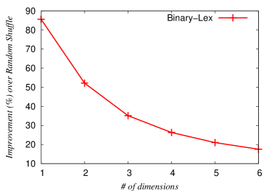
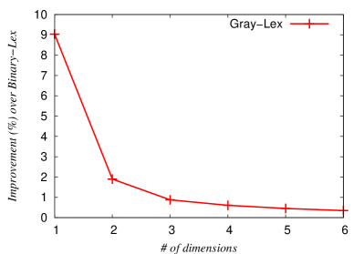
Our data sets have 100 attribute values per dimension, and the frequency of the attribute values is Zipfian (proportional to $1/r$, where $r$ is the rank of an item). Dimensions were independent of one another. See Fig. 9, where we compare Binary-Lex to an unsorted table, and then Gray-Lex to Binary-Lex. For the latter, the advantage drops quickly with the number of dimensions. For one dimension, the performance improvement is 9% for $k=2$, but for more than 2 dimensions, it is less than 2%. On other data sets, Gray-Lex either had no effect or a small positive effect.

Table 6: Total sizes (words) of 32-bit EWAH bitmaps for various sorting methods.

	k	Unsorted	Rand-Lex	Binary-Lex	Gray-Lex	Gray-Freq.
Census-	1	$8.49\times 10^{5}$	$4.87\times 10^{5}$	$4.87\times 10^{5}$	$4.87\times 10^{5}$	$4.87\times 10^{5}$
Income	2	$9.12\times 10^{5}$	$6.53\times 10^{5}$	$4.53\times 10^{5}$	$4.52\times 10^{5}$	$4.36\times 10^{5}$
(4d)	3	$6.90\times 10^{5}$	$4.85\times 10^{5}$	$3.77\times 10^{5}$	$3.73\times 10^{5}$	$3.28\times 10^{5}$
	4	$4.58\times 10^{5}$	$2.74\times 10^{5}$	$2.23\times 10^{5}$	$2.17\times 10^{5}$	$1.98\times 10^{5}$
DBGEN	1	$5.48\times 10^{7}$	$3.38\times 10^{7}$	$3.38\times 10^{7}$	$3.38\times 10^{7}$	$3.38\times 10^{7}$
(4d)	2	$7.13\times 10^{7}$	$2.90\times 10^{7}$	$2.76\times 10^{7}$	$2.76\times 10^{7}$	$2.74\times 10^{7}$
	3	$5.25\times 10^{7}$	$1.73\times 10^{7}$	$1.51\times 10^{7}$	$1.50\times 10^{7}$	$1.50\times 10^{7}$
	4	$3.24\times 10^{7}$	$1.52\times 10^{7}$	$1.21\times 10^{7}$	$1.21\times 10^{7}$	$1.19\times 10^{7}$
Netflix	1	$6.20\times 10^{8}$	$3.22\times 10^{8}$	$3.22\times 10^{8}$	$3.22\times 10^{8}$	$3.19\times 10^{8}$
	2	$8.27\times 10^{8}$	$4.18\times 10^{8}$	$3.17\times 10^{8}$	$3.17\times 10^{8}$	$2.43\times 10^{8}$
	3	$5.73\times 10^{8}$	$2.40\times 10^{8}$	$1.98\times 10^{8}$	$1.97\times 10^{8}$	$1.49\times 10^{8}$
	4	$3.42\times 10^{8}$	$1.60\times 10^{8}$	$1.39\times 10^{8}$	$1.37\times 10^{8}$	$1.14\times 10^{8}$
KJV-	1	$6.08\times 10^{9}$	$6.68\times 10^{8}$	$6.68\times 10^{8}$	$6.68\times 10^{8}$	$6.68\times 10^{8}$
4grams	2	$8.02\times 10^{9}$	$1.09\times 10^{9}$	$1.01\times 10^{9}$	$9.93\times 10^{8}$	$7.29\times 10^{8}$
	3	$4.13\times 10^{9}$	$9.20\times 10^{8}$	$8.34\times 10^{8}$	$8.31\times 10^{8}$	$5.77\times 10^{8}$
	4	$2.52\times 10^{9}$	$7.23\times 10^{8}$	$6.49\times 10^{8}$	$6.39\times 10^{8}$	$5.01\times 10^{8}$

Table 6 shows the sum of bitmap sizes using Gray-Lex orderings and Gray-Frequency. For comparison, we also used an unsorted table (the code allocation should not matter; we used the same code allocation as Binary-Lex), and we used a random code assignment with a lexicographically sorted table (Rand-Lex). Dimensions were ordered from the largest to the smallest (“4321”) except for Census-Income where we used the ordering “3214”.

KJV-4grams had a larger index for $k=2$ than $k=1$. This data set has many very long runs of identical attribute values in the first two dimensions, and the number of attribute values is modest, compared with the number of rows. This is ideal for 1-of-$N$.

For $k=1$, as expected, encoding is irrelevant: Rand-Lex, Binary-Lex, Gray-Lex, and Gray-Freq have identical results. However, sorting the table lexicographically is important: the reduction in size of the bitmaps is about 40% for 3 data sets (Census-Income, DBGEN, Netflix), and goes up to 90% for KJV-4grams.

For $k>1$, Gray-Frequency yields the smallest indexes in Table 6. The difference with the second-best, Gray-Lex, can be substantial (25%) but is typically small. However, Gray-Frequency is histogram-aware and thus, more complex to implement. The difference between Gray-Lex and Binary-Lex is small even though Gray-Lex is sometimes slightly better ($\approx$2%) especially for denser indexes ($k=4$). However, Rand-Lex is noticeably worse (up to $\approx$25%) than both of them: this means that encoding is a significant issue. All three schemes (Binary-Lex, Gray-Lex, Rand-Lex) have about the same complexity—all three are histogram-oblivious—and therefore Gray-Lex is recommended.

We omit Frequent-Component from the table. On Netflix, for $k=1$, it outperformed the other approaches by 1%, and for DBGEN it was only slightly worse than the others. But in all other case on DBGEN, Census-Income and Netflix, it lead to indexes 5–50% larger. (For instance, on Netflix ($k=4$) the index size was $1.52\times 10^{8}$ words, barely better than Rand-Lex and substantially worse than Gray-Frequency.) Because it interleaves attribute values and it is histogram-aware, it may be the most difficult scheme to implement efficiently among our candidates. Hence, we recommend against Frequent-Component.

7.7 Column effects

We experimentally evaluated how lexicographic sorting affects the EWAH compression of individual columns. Whereas sorting tends to create runs of identical values in the first columns, the benefits of sorting are far less apparent in later columns, except those strongly correlated with the first few columns. For Table 7, we have sorted projections of Census-Income and DBGEN onto 10 dimensions $d_{1}\ldots{}d_{10}$ with $n_{1}<\ldots<n_{10}$. (The dimensions $d_{1}\ldots d_{4}$ in this group are different from the dimensions $d_{1}\ldots d_{4}$ discussed earlier.) We see that if we sort from the largest column ($d_{10}\ldots{}d_{1}$), at most 3 columns benefit from the sort, whereas 5 or more columns benefit when sorting from the smallest column ($d_{1}\ldots{}d_{10}$).

Table 7: Number of 32-bit words used for different unary indexes when the table was sorted lexicographically (dimensions ordered by descending cardinality, $d_{10}\ldots d_{1}$, or by ascending cardinality, $d_{1}\ldots d_{10}$).

	cardinality	unsorted	$d_{1}\ldots d_{10}$	$d_{10}\ldots d_{1}$
$d_{1}$	7	42 427	32	42 309
$d_{2}$	8	36 980	200	36 521
$d_{3}$	10	34 257	1 215	28 975
$d_{4}$	47	0.13$\times 10^{6}$	12 118	0.13$\times 10^{6}$
$d_{5}$	51	35 203	17 789	28 803
$d_{6}$	91	0.27$\times 10^{6}$	75 065	0.25$\times 10^{6}$
$d_{7}$	113	12 199	9 217	12 178
$d_{8}$	132	20 028	14 062	19 917
$d_{9}$	1 240	29 223	24 313	28 673
$d_{10}$	99 800	0.50$\times 10^{6}$	0.48$\times 10^{6}$	0.30$\times 10^{6}$
total	-	1.11$\times 10^{6}$	0.64$\times 10^{6}$	0.87$\times 10^{6}$

(a) Census-Income

	cardinality	unsorted	$d_{1}\ldots d_{10}$	$d_{10}\ldots d_{1}$
$d_{1}$	2	0.75$\times 10^{6}$	24	0.75$\times 10^{6}$
$d_{2}$	3	1.11$\times 10^{6}$	38	1.11$\times 10^{6}$
$d_{3}$	7	2.58$\times 10^{6}$	150	2.78$\times 10^{6}$
$d_{4}$	9	0.37$\times 10^{6}$	1 006	3.37$\times 10^{6}$
$d_{5}$	11	4.11$\times 10^{6}$	10 824	4.11$\times 10^{6}$
$d_{6}$	50	13.60$\times 10^{6}$	0.44$\times 10^{6}$	1.42$\times 10^{6}$
$d_{7}$	2 526	23.69$\times 10^{6}$	22.41$\times 10^{6}$	23.69$\times 10^{6}$
$d_{8}$	200́00	24.00$\times 10^{6}$	24.00$\times 10^{6}$	22.12$\times 10^{6}$
$d_{9}$	400 000	24.84$\times 10^{6}$	24.84$\times 10^{6}$	19.14$\times 10^{6}$
$d_{10}$	984 297	27.36$\times 10^{6}$	27.31$\times 10^{6}$	0.88$\times 10^{6}$
total	-	0.122$\times 10^{9}$	0.099$\times 10^{9}$	$0.079\times 10^{9}$

(b) DBGEN

We also assessed how the total size of the index was affected by various column orderings; we show the Gray-Lex index sizes for each column ordering in Fig. 10. The dimensions of KJV-4grams are too similar for ordering to be interesting, and we have omitted them. For small dimensions, the value of $k$ was lowered using the heuristic presented in § 2. Our results suggest that table-column reordering has a significant effect (40%).

The value of $k$ affects which ordering leads to the smallest index: good orderings for $k=1$ are frequently bad orderings for $k>1$, and vice versa. This is consistent with our earlier analysis (see Figs. 7 and 8). For Netflix and DBGEN, we have omitted $k=2$ for legibility.

(a) Census-Income

(b) DBGEN

(c) Netflix

Figure 10: Sum of EWAH bitmap sizes (words, $y$ axis) on 4-d data sets for all dimension orderings ($x$ axis).

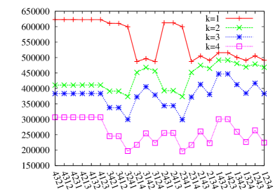
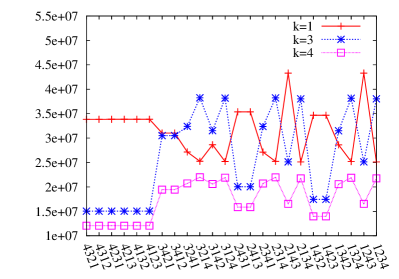
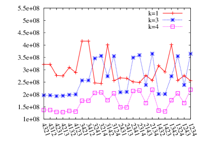
Census-Income’s largest dimension is very large ($n_{4}\approx n/2$); DBGEN also has a large dimension ($n_{4}\approx n/35$). Sorting columns in decreasing order with respect to $\min(n_{i}^{-1/k},(1-n_{i}^{-1/k})/(4w-1))$ for $k=1$, we have that only for DBGEN the ordering “2134” is suggested, otherwise, “1234” (from smallest to largest) is recommended. Thus the heuristic provides nearly optimal recommendations. For $k=3$ and $k=4$, the ordering “1234” is recommended for all data sets: for $k=4$ and Census-Income, this recommendation is wrong. For $k=2$ and Census-Income, the ordering “3214” is recommended, another wrong recommendation for this data set. Hence, a better column reordering heuristic is needed for $k>1$. Our greedy approach may be too simple, and it may be necessary to know the histogram skews.

7.8 Index size growth

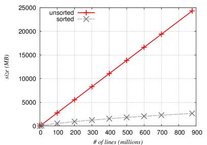
To study scaling, we built indexes from prefixes of the full KJV-4grams data set. We found that the sum of the EWAH bitmap sizes (see Fig. 11) increased linearly. Yet with sorting, the bitmap sizes increased sublinearly. As new data arrives, it is increasingly likely to fit into existing runs, once sorted. Hence—everything else being equal—sorting becomes more beneficial as the data sets grow.

Figure 11: Sum of the EWAH bitmap sizes for various prefixes of the KJV-4grams table ($k=1$)

7.9 Bitmap reordering

Sharma and Goyal [7] consider encoding a table into a bitmap index using a multi-component code (similar to $k$-of-$N$), then GC sorting the rows of the index, and finally applying WAH compression. Canahuate et al. [10] propose a similar approach, with the additional step of permuting the columns—meaning the individual bitmaps—in the index prior to GC sorting. For example, whereas the list of 2-of-4 codes in increasing GC order is 0011, 0110, 0101, 1100, 1010, 1001, by permuting the first and the last bit, we obtain the following (non-standard) Gray code: 1010, 0110, 1100, 0101, 0011, 1001. In effect, reordering bitmaps is equivalent to sorting the (unpermuted) index rows according to a non-standard Gray code. They chose to use bitmap density to determine which index columns should come first, but reported that the different orders had little effect on the final index sizes.

In contrast, our approach has been to permute the columns of the table—not the individual bitmaps, then sort the table lexicographically, and finally generate the compressed index. Permuting the attributes corresponds to permuting blocks of bitmaps: our bitmap permutations are a special case of Canahaute’s. We do not know a sufficiently efficient method to sort our largest data sets with arbitrary bitmap reordering. We cannot construct the uncompressed index: for KJV-4grams, we would require at least 3.7 TB. Instead, we used the compressed B-tree approach mentioned in § 5.1 and applied the bitmap permutation to its keys. This was about 100 times slower than our normal Gray-Lex method, and implementation restrictions prevented our processing the full Netflix or KJV-4grams data sets. Hence, we took the first 20 million records from each of these two data sets, forming Netflix20M and KJV20M.

Our experiments showed that little compression was lost by restricting ourselves to the special case of permuting table columns, rather than individual bitmaps. While we indexed all the $4!=24$ tables generated by all column permutations in our 4-column data sets, it is infeasible to consider all bitmap permutations. Even if there were only 100 bitmaps, the number of permutations would be prohibitively large ($100!\approx 10^{158}$). We considered three heuristics based on bitmap density $\cal D$—the number of 1-bits over the total number of bits ($n$) :

1. “Incompressible first” (IF), which orders bitmaps by increasing $|\,{\cal D}-0.5\,|$. In other words, bitmaps with density near 0.5 are first [10].

2. “Moderately sparse first” (MSF), ordering by the value $\min({\cal D},\frac{1-{\cal D}}{4\times 32-1})$ as discussed at the end of § 5.3. This is a per-bitmap variant of the column-reordering heuristic we evaluate experimentally in § 7.7.

3. “Sparse first” (SF): order by increasing ${\cal D}$.

Results are shown in Table 8. In only one case (KJV20M, $k=1$), was a per-bitmap result significantly better (by 5%) than our default method of rearranging table columns instead of individual bitmaps. In most other cases, all per-bitmap reorderings were worse, sometimes by large factors (30%).

IF ordering performs poorly when there are some dense bitmaps (i.e., when $k>1$.) Likewise, SF performs poorly for sparse bitmaps ($k=1$). We do not confirm prior reports [10] that index column order has relatively little effect on the index size: on our data, it makes a substantial difference. Perhaps the characteristics of their scientific data sets account for this difference.

Table 8: Sum of the EWAH bitmap sizes (in words), GC sorting and various bitmap orders

		Best column	Per-bitmap reordering
		order	IF	MSF	SF
Census-Income	$k=1$	$4.87\times 10^{5}$	$4.91\times 10^{5}$	$4.91\times 10^{5}$	$6.18\times 10^{5}$
(4d)	2	$3.74\times 10^{5}$	$4.69\times 10^{5}$	$4.10\times 10^{5}$	$3.97\times 10^{5}$
	3	$2.99\times 10^{5}$	$3.83\times 10^{5}$	$3.00\times 10^{5}$	$3.77\times 10^{5}$
	4	$1.96\times 10^{5}$	$3.02\times 10^{5}$	$\mathbf{1.91\times 10^{5}}$	$\mathbf{1.91\times 10^{5}}$
DBGEN	1	$2.51\times 10^{7}$	$2.51\times 10^{7}$	$2.51\times 10^{7}$	$3.39\times 10^{7}$
(4d)	2	$2.76\times 10^{7}$	$4.50\times 10^{7}$	$4.35\times 10^{7}$	$2.76\times 10^{7}$
	3	$1.50\times 10^{7}$	$3.80\times 10^{7}$	$1.50\times 10^{7}$	$1.50\times 10^{7}$
	4	$1.21\times 10^{7}$	$2.18\times 10^{7}$	$1.21\times 10^{7}$	$1.21\times 10^{7}$
Netflix20M	1	$5.48\times 10^{7}$	$5.87\times 10^{7}$	$5.87\times 10^{7}$	$6.63\times 10^{7}$
	2	$7.62\times 10^{7}$	$9.05\times 10^{7}$	$8.61\times 10^{7}$	$7.64\times 10^{7}$
	3	$4.43\times 10^{7}$	$7.99\times 10^{7}$	$\mathbf{4.39\times 10^{7}}$	$\mathbf{4.39\times 10^{7}}$
	4	$2.99\times 10^{7}$	$4.82\times 10^{7}$	$3.00\times 10^{7}$	$3.00\times 10^{7}$
KJV20M	1	$4.06\times 10^{7}$	$4.85\times 10^{7}$	$4.83\times 10^{7}$	$\mathbf{3.85\times 10^{7}}$
	2	$5.77\times 10^{7}$	$6.46\times 10^{7}$	$\mathbf{5.73\times 10^{7}}$	$\mathbf{5.73\times 10^{7}}$
	3	$3.95\times 10^{7}$	$4.47\times 10^{7}$	$4.24\times 10^{7}$	$4.24\times 10^{7}$
	4	$2.72\times 10^{7}$	$3.42\times 10^{7}$	$3.38\times 10^{7}$	$3.38\times 10^{7}$

7.10 Queries

We implemented queries over the bitmap indexes by processing the logical operations two bitmaps at a time: we did not use Algorithm 3. Bitmaps are processed in sequential order, without sorting by size, for example. The query processing costs includes the extraction of the row IDs—the location of the 1-bits—from the bitmap form of the result.

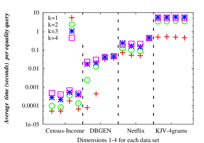
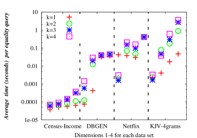
We timed equality queries against our 4-d bitmap indexes. Recall that dimensions were ordered from the largest to the smallest (4321) except for Census-Income where we used the ordering “3214.” Gray-Lex encoding is used for $k>1$. Queries were generated by choosing attribute values uniformly at random and the figures report average wall-clock times for such queries. We made 100 random choices per column for KJV-4grams when $k>1$. For DBGEN and Netflix, we had 1 000 random choices per column and 10 000 random choices were used for Census-Income and KJV-4grams ($k=1$). For each data set, we give the results per column (leftmost tick is the column used as the primary sort key, next tick is for the secondary sort key, etc.). The results are shown in Fig. 12.

From Fig. 12(b), we see that simple bitmap indexes almost always yield the fastest queries. The difference caused by $k$ is highly dependent upon the data set and the particular column in the data set. However, for a given data set and column, with only a few small exceptions, query times increase with $k$, especially from $k=1$ to $k=2$. For DBGEN, the last two dimensions have size 7 and 11, whereas for Netflix, the last dimension has size 5, and therefore, they will never use a $k$-value larger than 2: their speed is mostly oblivious to $k$.

An exception occurs for the first dimension of Netflix, and it illustrates the importance of benchmarking with large data sets. Note that using $k=1$ is much slower than using $k>1$. However, these tests were done using a disk whose access typically requires at least 18 ms. In other words, any query answered substantially faster than 20 ms was answered without retrieving data from the disk platter (presumably, it came from the operating system’s cache, or perhaps the disk’s cache). For $k>1$, it appears that the portion of the index for the first attribute (which is $\approx 7$ MB) could be cached successfully, whereas for $k=1$, the portion of the index was 100 MB and could not be cached.

In § 6, we predicted that the query time would grow with $k$ as $\approx(2-1/k)n_{i}^{-1/k}$: for the large dimensions such as the largest ones for DBGEN (400k) and Netflix (480k), query times are indeed significantly slower for $k=2$ as opposed to $k=1$. However, our model exaggerates the differences by an order of magnitude. The most plausible explanation is that query times are not proportional to the sizes of the bitmap loaded, but also include a constant factor. This may correspond to disk access times.

Fig. 12(a) and 12(b) also show the equality query times per column before and after sorting the tables. Sorting improves query times most for larger values of $k$: for Netflix, sorting improved the query times by

• at most 2 for $k=1$,

• at most 50 for $k=2$,

• and at most 120 for $k=3$.

This is consistent with our earlier observation that indexes with $k>1$ benefit from sorting even when there are no long runs of identical values (see § 5.1). (On the first columns, $k=3$ usually gets the best improvements from sorting.) The synthetic data set DBGEN showed no significant speedup from sorting, beyond its large first column. Although Netflix, like DBGEN, has a many-valued column first, it shows a benefit from sorting even in its third column: in fact, the third column benefits more from sorting than the second column. The largest table, KJV-4grams, benefited most from the sort: while queries on the last column are up to 10 times faster, the gain on the first two columns ranges from 125 times faster ($k=1$) to almost 3 300 times faster ($k=3$).

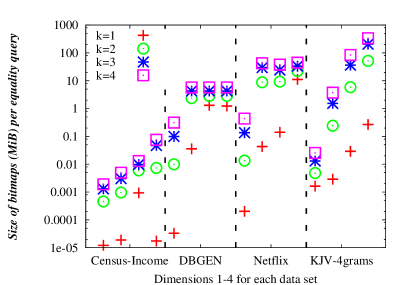
We can compare these times with the expected amount of data scanned per query. This is shown in Fig. 13, and we observe some agreement between most query times and the expected sizes of the bitmaps being scanned. The most notable exceptions are for $k=1$; in many such cases we must make an expensive seek far into a file for a very small compressed bitmap. Moreover, a small compressed bitmap may, via long runs of 1x11 clean words, represent many row IDs. To answer the query, we must still produce the set of row IDs.

(a) Unsorted table

(b) Sorted table and Gray-Lex encoding

Figure 12: Query times are affected by dimension, table sorting and $k$.

Figure 13: Bitmap data examined per equality query.

7.11 Effect of the word length

Our experiments so far use 32-bit EWAH. To investigate the effect of word length, we recompiled our executables as 64-bit binaries and implemented 16-bit and 64-bit EWAH. The index sizes are reported in Table 10(b)—the index size excludes a B-Tree storing maps from attribute values to bitmaps. We make the following observations:

• 16-bit indexes can be 10 times larger than 32-bit indexes.

• 64-bit indexes are nearly twice as large as 32-bit indexes.

• Sorting benefits 32-bit and 64-bit indexes equally; 16-bit indexes do not benefit from sorting.

Despite the large variations in file sizes, the difference between index construction times (omitted) in 32-bit and 64-bit indexes is within 5%. Hence, index construction is not bound by disk I/O performance.

Table 9: Index size (file size in MB) for unary bitmap indexes ($k=1$) under various word lengths. For Census-Income and DBGEN, the 4-d projection is used.

	index size (MB)
word length	Census-Income	DBGEN	Netflix	KJV-4grams
16	12.0	2.5$\times 10^{3}$	2.6$\times 10^{4}$	2.6$\times 10^{4}$
32	3.8	221	2.5$\times 10^{3}$	2.4$\times 10^{4}$
64	6.5	416	4.8$\times 10^{3}$	4.4$\times 10^{4}$

(a) Unsorted

	index size (MB)
word length	Census-Income	DBGEN	Netflix	KJV-4grams
16	11.1	2.4$\times 10^{3}$	2.5$\times 10^{4}$	1.6$\times 10^{4}$
32	2.9	137	1.3$\times 10^{3}$	2.6$\times 10^{3}$
64	4.8	227	2.2$\times 10^{3}$	4.3$\times 10^{3}$

(b) Lexicographically sorted

7.12 Range queries

Unary bitmap indexes may not be ideally suited for all ranges queries [22]. However, range queries are good stress tests: they require loading and computing numerous bitmaps. Our goal is to survey the effect of sorting and word length on the aggregation of many bitmaps.

We implemented range queries using the following simple algorithm:

1. For each dimension, we compute the logical OR of all matching bitmaps. We aggregate the bitmaps two at time: $((B_{1}\lor B_{2})\lor B_{3})\lor B_{4})\ldots$ When there are many bitmaps, Algorithm 3 or an in-place algorithm might be faster. (See Wu et al. [27, 3] for a detailed comparison of pair-at-a-time versus in-place processing.)

2. We compute the logical AND of all the dimensional bitmaps—resulting from the previous step.

We implemented a flag to disable the aggregation of the bitmaps to measure solely the cost of loading the bitmaps in memory. (Our implementation does not write its temporary results to disk.) We omitted 16-bit EWAH from our tests due to its poor compression rate.

As a basis for comparison, we also implemented range queries using uncompressed external-memory B-tree [35] indexes over each column: the index maps values to corresponding row IDs. The computation is implemented as with the bitmaps, using the STL functions set_intersection and set_union. We required row IDs to be provided in sorted order. All query times were at least an order of magnitude larger than with 32-bit or 64-bit bitmap indexes. We failed to index the columns with uncompressed B-trees in a reasonable time (a week) over the KJV-4grams data set due to the large file size (21.6 GB).

We generated a set of uniformly randomly distributed 4-d range queries using no more than 100 bitmaps per dimension. We used the same set of queries for all indexes. The results are presented in Table 11(b). Our implementation of range queries using uncompressed B-tree indexes is an order of magnitude slower than the bitmap indexes over Netflix, hence we omit the results.

The disk I/O can be nearly twice as slow with 64-bit indexes and KJV-4grams. However, disk I/O is negligible, accounting for about 1% of the total time.

The 64-bit indexes are nearly twice as large. We expect that 64-bit indexes also generate larger intermediate bitmaps during the computation. Yet, the 64-bit indexes have faster overall performance: 40% for DBGEN and 5% for other cases, except for sorted KJV-4grams where the gain was 18%. Moreover, the benefits of 64-bit indexes are present in both sorted and unsorted indexes.

Table 10: Average 4-d range query processing time over the Netflix data set for unary bitmap indexes ($k=1$) under various word lengths and dimensional B-tree indexes.

DBGEN	unsorted	lexicographically sorted
32-bit EWAH	0.382	0.378
64-bit EWAH	0.273	0.265
Netflix
32-bit EWAH	2.87	1.50
64-bit EWAH	2.67	1.42
KJV-4grams
32-bit EWAH	44.8	5.2
64-bit EWAH	42.4	4.4

(a) Average wall-clock query time (s)

DBGEN	unsorted	lexicographically sorted
32-bit EWAH	0.023	0.023
64-bit EWAH	0.027	0.026
Netflix
32-bit EWAH	0.11	0.078
64-bit EWAH	0.16	0.097
KJV-4grams
32-bit EWAH	0.57	0.06
64-bit EWAH	1.11	0.1

(b) Average disk I/O time (s)

8 Guidelines for k

Our experiments indicate that simple ($k=1$) bitmap encoding is preferable when storage space and index-creation time are less important than fast equality queries. The storage and index-creation penalties are kept modest by table sorting and Algorithm 1.

Space requirements can be reduced by choosing $k>1$, although Table 6 shows that this approach has risks (see KJV-4grams). For $k>1$, we can gain additional index size reduction at the cost of longer index construction by using Gray-Frequency rather than Gray-Lex.

If the total number of attribute values is small relative to the number of rows, then we should first try the $k=1$ index. Perhaps the data set resembles KJV-4grams. Besides yielding faster queries, the $k=1$ index may be smaller.

9 Conclusion and future work

We showed that while sorting improves bitmap indexes, we can improve them even more (30–40%) if we know the number of distinct values in each column. For $k$-of-$N$ encodings with $k>1$, even further gains (10–30%) are possible using the frequency of each value. Regarding future work, the accurate mathematical modelling of compressed bitmap indexes remains an open problem. While we only investigated bitmap indexes, we can generalize this work in the context of column-oriented databases [47, 48] by allowing various types of indexes.

Daniel Lemire received a B.Sc. and a M.Sc. in Mathematics from the University of Toronto in 1994 and 1995. He received his Ph.D. in Engineering Mathematics from the Ecole Polytechnique and the Université de Montréal in 1998. He is now a professor at the Université du Québec à Montréal (UQAM) where he teaches Computer Science. His research interests include data warehousing, OLAP and time series.

Owen Kaser is Associate Professor in the Department of Computer Science and Applied Statistics, at the Saint John campus of The University of New Brunswick. He received a Ph.D. in Computer Science in 1993 from SUNY Stony Brook.

Kamel Aouiche graduated as an engineer from the University Mouloud Mammeri in 1999, he received a B.Sc. in Computer Science from the INSA de Lyon in 2002 and a Ph.D. from the Université Lumière Lyon 2 in 2005. He completed a post-doctoral fellowship at Université du Québec à Montréal (UQAM) in 2008. Currently, he works as a consultant in industry.

References

- [1] L. Bellatreche, R. Missaoui, H. Necir, H. Drias, Selection and pruning algorithms for bitmap index selection problem using data mining, in: DaWaK 2007 (LNCS 4654), Springer, 2007, pp. 221–230.
- [2] K. Davis, A. Gupta, Data Warehouses and OLAP: Concepts, Architectures, and Solutions, IRM Press, 2007, Ch. Indexing in Data Warehouses.
- [3] K. Wu, E. J. Otoo, A. Shoshani, Optimizing bitmap indices with efficient compression, ACM Transactions on Database Systems 31 (1) (2006) 1–38.
- [4] C. Y. Chan, Y. E. Ioannidis, Bitmap index design and evaluation, in: SIGMOD’98, 1998, pp. 355–366.
- [5] G. Antoshenkov, Byte-aligned bitmap compression, in: DCC’95, 1995, p. 476.
- [6] K. Wu, E. J. Otoo, A. Shoshani, A performance comparison of bitmap indexes, in: CIKM ’01, 2001, pp. 559–561.
- [7] Y. Sharma, N. Goyal, An efficient multi-component indexing embedded bitmap compression for data reorganization, Information Technology Journal 7 (1) (2008) 160–164.
- [8] T. Apaydin, A. Şaman Tosun, H. Ferhatosmanoglu, Analysis of basic data reordering techniques, in: SSDBM 2008, LNCS 5096, 2008, pp. 517–524.
- [9] A. Pinar, T. Tao, H. Ferhatosmanoglu, Compressing bitmap indices by data reorganization, in: ICDE’05, 2005, pp. 310–321.
- [10] G. Canahuate, H. Ferhatosmanoglu, A. Pinar, Improving bitmap index compression by data reorganization, http://hpcrd.lbl.gov/~apinar/papers/TKDE06.pdf (checked 2008-12-15) (2006).
- [11] O. Kaser, D. Lemire, K. Aouiche, Histogram-aware sorting for enhanced word-aligned compression in bitmap indexes, in: DOLAP ’08, 2008.
- [12] P. E. O’Neil, Model 204 architecture and performance, in: 2nd International Workshop on High Performance Transaction Systems, 1989, pp. 40–59.
- [13] J. Hammer, L. Fu, CubiST++: Evaluating ad-hoc CUBE queries using statistics trees, Distributed and Parallel Databases 14 (3) (2003) 221–254.
- [14] V. Sharma, Bitmap index vs. b-tree index: Which and when?, online: http://www.oracle.com/technology/pub/articles/sharma_indexes.html (March 2005).
- [15] R. Weber, H.-J. Schek, S. Blott, A quantitative analysis and performance study for similarity-search methods in high-dimensional spaces, in: VLDB ’98, 1998, pp. 194–205.
- [16] K. Aouiche, D. Lemire, A comparison of five probabilistic view-size estimation techniques in OLAP, in: DOLAP’07, 2007, pp. 17–24.
- [17] H. K. T. Wong, H. F. Liu, F. Olken, D. Rotem, L. Wong, Bit transposed files, in: VLDB 85, 1985, pp. 448–457.
- [18] N. Koudas, Space efficient bitmap indexing, in: CIKM ’00, 2000, pp. 194–201.
- [19] D. Rotem, K. Stockinger, K. Wu, Minimizing I/O costs of multi-dimensional queries with bitmap indices, in: SSDBM ’06, 2006, pp. 33–44.
- [20] K. Stockinger, K. Wu, A. Shoshani, Evaluation strategies for bitmap indices with binning, in: DEXA ’04, 2004.
- [21] R. Darira, K. C. Davis, J. Grommon-Litton, Heuristic design of property maps, in: DOLAP’06, 2006, pp. 91–98.
- [22] R. R. Sinha, M. Winslett, Multi-resolution bitmap indexes for scientific data, ACM Trans. Database Syst. 32 (3) (2007) 16.
- [23] R. Pagh, S. S. Rao, Secondary indexing in one dimension: Beyond b-trees and bitmap indexes, available from http://arxiv.org/abs/0811.2904 (2008).
- [24] K. Stockinger, K. Wu, A. Shoshani, Strategies for processing ad hoc queries on large data warehouses, in: DOLAP’02, 2002, pp. 72–79.
- [25] K. Wu, E. J. Otoo, A. Shoshani, H. Nordberg, Notes on design and implementation of compressed bit vectors, Tech. Rep. LBNL/PUB-3161, Lawrence Berkeley National Laboratory, available from http://crd.lbl.gov/~kewu/ps/PUB-3161.html (2001).
- [26] M. Jurgens, H. J. Lenz, Tree based indexes versus bitmap indexes: A performance study, International Journal of Cooperative Information Systems 10 (3) (2001) 355–376.
- [27] K. Wu, E. Otoo, A. Shoshani, On the performance of bitmap indices for high cardinality attributes, in: VLDB’04, 2004, pp. 24–35.
- [28] N. Christofides, Worst-case analysis of a new heuristic for the travelling salesman problem, Tech. Rep. 388, Graduate School of Industrial Administration, Carnegie Mellon University (1976).
- [29] A. Pinar, M. T. Heath, Improving performance of sparse matrix-vector multiplication, in: Supercomputing ’99, 1999.
- [30] G. Graefe, Implementing sorting in database systems, ACM Comput. Surv. 38 (3) (2006) 10.
- [31] J. Yiannis, J. Zobel, Compression techniques for fast external sorting, The VLDB Journal 16 (2) (2007) 269–291.
- [32] J. Cai, R. Paige, Using multiset discrimination to solve language processing problems without hashing, Theoretical Computer Science 145 (1-2) (1995) 189–228.
- [33] J. Ernvall, On the construction of spanning paths by Gray-code in compression of files, TSI. Technique et science informatiques 3 (6) (1984) 411–414.
- [34] D. Richards, Data compression and Gray-code sorting, Information processing letters 22 (4) (1986) 201–205.
- [35] M. Hirabayashi, QDBM: Quick database manager, http://qdbm.sourceforge.net/ (checked 2008-02-22) (2006).
- [36] D. E. Knuth, The Art of Computer Programming, Vol. 4, Addison Wesley, 2005, Ch. fascicle 2.
- [37] L. Goddyn, P. Gvozdjak, Binary gray codes with long bit runs, Electronic Journal of Combinatorics 10 (R27) (2003) 1–10.
- [38] C. Savage, P. Winkler, Monotone gray codes and the middle levels problem, Journal of Combinatorial Theory, A 70 (2) (1995) 230–248.
- [39] Hitachi Global Storage Technologies, Deskstar P7K500, http://www.hitachigst.com/tech/techlib.nsf/techdocs/30C3F554C477835B862%57377006E61A0/$file/HGST_Deskstar_P7K500_DS_FINAL.pdf (last checked 2008-12-21).
- [40] Dell, Specifications: Hitachi Deskstar P7K500 User’s Guide, https://support.dell.com/support/edocs/storage/P160227/specs.htm (last checked 2008-12-21).
- [41] S. Hettich, S. D. Bay, The UCI KDD archive, http://kdd.ics.uci.edu (checked 2008-04-28) (2000).
- [42] TPC, DBGEN 2.4.0, http://www.tpc.org/tpch/ (checked 2007-12-4) (2006).
- [43] Netflix, Inc., Nexflix prize, http://www.netflixprize.com (checked 2008-04-28) (2007).
- [44] Project Gutenberg Literary Archive Foundation, Project Gutenberg, http://www.gutenberg.org/ (checked 2007-05-30) (2007).
- [45] M. F. Porter, An algorithm for suffix stripping, in: Readings in information retrieval, Morgan Kaufmann, 1997, pp. 313–316.
-
[46]
O. Kaser, S. Keith, D. Lemire,
The LitOLAP project: Data warehousing with literature, in: CaSTA’06, 2006.
URL http://www.daniel-lemire.com/fr/documents/publications/%casta06_web.pdf - [47] M. Stonebraker, D. J. Abadi, A. Batkin, X. Chen, M. Cherniack, M. Ferreira, E. Lau, A. Lin, S. Madden, E. O’Neil, P. O’Neil, A. Rasin, N. Tran, S. Zdonik, C-store: a column-oriented DBMS, in: VLDB’05, 2005, pp. 553–564.
- [48] D. Abadi, S. Madden, M. Ferreira, Integrating compression and execution in column-oriented database systems, in: SIGMOD ’06, 2006, pp. 671–682.
![[Uncaptioned image]](/html/0901.3751/assets/pictureofdaniellemire.jpg)