Discovery of 28 pulsars using new techniques for sorting pulsar candidates

Abstract

Modern pulsar surveys produce many millions of candidate pulsars, far more than can be individually inspected. Traditional methods for filtering these candidates, based upon the signal-to-noise ratio of the detection, cannot easily distinguish between interference signals and pulsars. We have developed a new method of scoring candidates using a series of heuristics which test for pulsar-like properties of the signal. This significantly increases the sensitivity to weak pulsars and pulsars with periods close to interference signals. By applying this and other techniques for ranking candidates from a previous processing of the Parkes Multi-beam Pulsar Survey, 28 previously unknown pulsars have been discovered. These include an eccentric binary system and a young pulsar which is spatially coincident with a known supernova remnant.

1 Background

The Parkes Multi-beam Pulsar Survey (PMPS) is the most successful large-scale pulsar survey ever undertaken. Processing and re-processing of the PMPS data set has led to the discovery and publication of more than 750 previously unknown pulsars. A full description of the survey and the discoveries to date are outlined in the following papers. Manchester et al. (2001) discussed the hardware and software configuration for the survey and presented the first 100 new pulsars. Morris et al. (2002) provided details of a further 120 pulsars, and performed an initial statistical analysis of the the discovered pulsars. Two hundred more discoveries, including young pulsars and their association with EGRET sources are discussed by Kramer et al. (2003). Hobbs et al. (2004) presented a further 180 discoveries and discussed the detection of 281 previously-known pulsars in the survey. A complete re-processing of the survey data using new search algorithms was presented by Faulkner et al. (2004), hereafter known as the 2002 re-processing. Lorimer et al. (2006) presented 142 discoveries resulting from that analysis and performed a detailed statistical study of the pulsar population in the survey region. Most recently McLaughlin et al. (2006) detected 11 new transient radio pulsars, the RRATs which are only detected through their single pulses.

Section 2 describes new techniques for selecting candidate pulsars for re-observation from the many millions of candidates that are produced in the processing of a large-scale pulsar survey. In Section 3 we describe how we applied these techniques to the candidates from the 2002 re-processing and produced a short-list of 44 new candidates. These candidates were re-observed and yielded 28 previously unknown pulsars. Full astrometric and spin parameters for each of the newly discovered pulsars have been measured and are included in Section 4. Additionally we discuss two of the notable discoveries in detail. To determine the effectiveness of the new selection techniques, Section 5 includes a statistical comparison of the new discoveries and those presented by Faulkner et al. (2004).

2 Candidate selection

In a typical pulsar survey hundreds of pulsar candidates are generated by the search software for each beam in the survey. With large surveys, this can add up to millions of candidate pulsars. Each candidate consists of a selection of candidate parameters, which include the optimised period and dispersion measure (DM) of the pulsar as well as the signal-to-noise ratio as detected in the various search methods. Additionally, an number of diagnostic plots are generated from the time-series data, including a folded profile of the pulsar, the variation of signal-to-noise ratio with DM and plots showing the variation of pulse profile with time and observing frequency. These parameters and plots are used to select the candidate pulsars that are to be re-observed.

Figure 1: An example display of the data generated for a single candidate produced in a pulsar search. This plot shows the detection of the known pulsar PSR J1754–3443. The three plots on the left hand side are: the sub-bands plot, showing the four stacked profiles at different observing frequencies; the sub-integrations plot, indicating how the folded pulse profile is varying with time; and the pulse profile, folded at the optimal period and DM. On the right of the figure are two plots: The period-DM diagram, which shows the variation of signal-to-noise ratio with small changes in folding period; and DM and the DM curve, which shows the variation of signal-to-noise ratio over a large range of DM values. Also included are the pre and post-optimisation parameters and some basic header information about the observation.

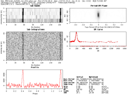
During the 2002 re-processing of the PMPS, candidates were selected for re-observation using Reaper, a graphical selection tool described by Faulkner et al. (2004). In brief, Reaper presents each candidate pulsar as a single point on a phase-space diagram. This diagram shows many thousands of candidates as a two-dimensional graph showing, for example, period on the x-axis and signal-to-noise ratio on the y-axis. This aids the selection of candidate points that are sufficiently distinguished from noise and interference signals. Selection of a point on this display causes the details of the selected candidate to be displayed to the user who can then make a decision regarding whether the candidate should be re-observed. An example of the plots that are presented when viewing the full candidate details are shown in Figure 1.

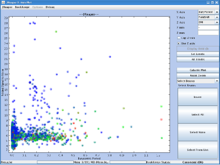
Following on the success of Reaper, a new software tool, JReaper, has been developed. This new tool has been developed to provide the functionality of Reaper, as well as advanced new functionality, on a wider range of data formats. This has been achieved by using a modular design which uses generic interfaces to read and write many different data formats. This allows for JReaper to be used on many different surveys and data archives without any significant changes to the core code base. Figure 2 shows a screen grab from an example session with JReaper, in this case showing candidate pulsars on a plot of barycentric period and folded signal-to-noise ratio.

JReaper has a number of features that have been developed to help pulsar searching. These include many simple functions, such as tracking viewed candidates and filtering displayed candidates by user selectable parameters (for example, hiding candidates with a DM of less than some value). The rest of this section provides details on some of the new, more advanced, functions of JReaper.

Figure 2: A typical JReaper display showing a number of candidates plotted with barycentric period verses signal-to-noise ratio. Each point is a pulsar candidate, and is coloured according to a third parameter (in this case the peak DM). Clicking on a candidate brings up a window showing full details of the candidate, including the diagnostic plots, and gives options to mark the candidate as a potential target for follow-up observations.

2.1 Scoring

Whilst the human-eye aspects of pulsar searching cannot easily be replicated by a machine, it is possible to detect some of the basic indicators used by human observers to distinguish real pulsars from interference. JReaper features a scoring algorithm that attempts to do this by assigning a numerical score to each candidate pulsar signal based on the data that are produced by the search algorithms. The scoring routine uses a number of tests that are then combined with weights to give a final score. The tests currently used are as follows:

2.1.1 Sub-integration scoring

Typical pulsars have a period and profile shape that are completely stable over the observation time, whereas for periodic man-made signals the period is often more variable. Periodic signals can be identified by eye by looking for straight lines running down a plot of pulse phase vs observation time, known as the sub-integration plot. We have investigated a number of ways to automate this process.

1. 2-Dimensional Kolmogorov-Smirnov Test – The Kolmogorov-Smirnov test provides a statistical way to determine if two data sets differ from one another significantly. This can be applied to the sub-integrations by comparing the observed values with a sample set generated from Gaussian noise. Any significant deviation implies that the signal is not due simply to noise. Whilst effective at discriminating between signals and noise, this test is not effective at differentiating between interference signals and real pulsar signals. It is also ineffective when the pulse is weak enough that there is not a significant signal in each sub-integration. For these reasons the Kolmogorov-Smirnov Test was not used in the final version of JReaper.

2. Hough Transform – Under the Hough transform, the input data is mapped in terms of any set of parametrised curves Hough (1960); Duda & Hart (1972). For the purpose of finding straight lines this means showing the data as a plot of how much power lies on each line with a given slope and intercept. This can be used to simplify the problem of finding a straight line down the sub-integrations to that of finding a discrete significant peak in the Hough transformed plane. In this case, each slope corresponds to an error in the folding period and intercept to a phase bin of the profile. This can be generalised to any polynomial to fit accelerated sources, where the pulse phase drifts non-linearly with time, although the dimensionality of the Hough plane increases with each extra power. This method is effective at removing signals that are not caused by strictly periodic sources, and is not dependant on the strength of the signal in each sub-integration. However the Hough transform is computationally expensive and is effectively repeating work that was already done as part of the time domain optimisation. The Hough transform is computationally equivalent to the period adjustment performed by sliding and adding the sub-integrations. This operation is performed during the final ‘time-domain optimisation’ step of typical pulsar search methods. Therefore with simple modifications to existing code, the Hough method can be applied to data without any extra processing cost.

3. Period curve scoring – This method considers the variation of signal-to-noise ratio with trial period as a marker of the periodicity in the sub-integrations. This works using a similar concept to the Hough transform, except the phase information is removed by computing the signal-to-noise ratio of each output profile. This one dimensional output is much simpler to score, as one can model the expected curve for a realistic source by:

   $$W_{\rm eff}=\sqrt{W_{\rm int}^{2}+(T_{\rm obs}\cdot\Delta{P}/P)^{2}},$$ (1)

   $$\frac{\rm Signal}{\rm Noise}\propto\sqrt{P-W_{\rm eff}\over W_{\rm eff}}.$$ (2)

   Here $P$ is the pulse period, $\Delta{P}$ is the offset in period, $W_{\rm int}$ is the intrinsic pulse width, assumed to be the pulse width at the optimised period. Note that if $W_{\rm eff}$ is greater than the period, it is assumed that the pulse is completely smeared, and the signal-to-noise ratio is 0.

   By computing the RMS deviation from the model curve, the observed curve can be scored, with low RMS scoring highly. This is the preferred method for scoring the sub-integrations as it a simple calculation and does not rely on any complex 2-dimensional analysis.

2.1.2 DM curve scoring

This scoring method considers how the detected signal-to-noise ratio varies with trial DM. Given a period, pulse width and observational frequency and bandwidth, it is possible to compute a theoretical variation of signal-to-noise ratio with DM, similar to that described for period offset above:

$$W_{\rm eff}=\sqrt{W_{\rm int}^{2}+(k_{\rm DM}\cdot\Delta{DM}\cdot\Delta{\nu}/\nu^{3})^{2}}.$$ (3)

Here $\Delta{DM}$ is the DM offset from the true DM (measured in cm^-3pc), $\Delta{\nu}$ is the total observation bandwidth (in MHz), $\nu$ is the observation frequency (also in MHz) and the constant $k_{\rm DM}=8.297616\times 10^{3}$ cm³pc^-1s^-1. $W_{\rm eff}$ can then be fed into equation 2 above. This model is then compared with the observed values by taking the RMS deviation from the theoretical values. To avoid bad scores from noise being detected at the same period, the DM-curve is only considered over the range of DM values for which the signal-to-noise ratio less than 20% of the peak signal-to-noise ratio. Candidates score highly if their RMS deviation is low.

2.1.3 Zero DM comparison

Some un-dispersed signals can be mis-detected at a high DM, caused when a signal with low variation with DM (i.e. a narrow band interference signal) is mixed with a noisy background. To identify these sources, the DM curve scoring is re-performed assuming that the source was at DM of zero. If the scoring is the same or better assuming zero DM then there is a high probability that the DM value has been overestimated. This routine returns a high score if the difference between the zero DM score and the optimised DM score is large.

2.1.4 Profile scoring

Profile scoring detects what fraction of the pulse is above a threshold of 60% of the peak value. This is designed to select against a common type of RFI which exhibits negative ‘pulses’, those that have troughs in power rather than peaks. This scoring method is tuned to start selecting against profiles which have more than 50% of their signal above the threshold.

2.1.5 Score combination

The result of each score is stored with each candidate, and the final score value that is used for plotting is computed based on user specified weights. These weights allow the user to display the results in multiple different views. For example, weighting the sub integration scoring highly removes a lot of interference, but also affects binary sources, so the user may choose to view the data twice, once with high weighting and once with a low weighting to the sub integration scoring.

Interference signals are often detected with a high signal-to-noise ratio, although typically they do not show the basic characteristics of a pulsar and therefore score relatively badly compared to a real pulsar signal. The scoring functions are tuned to select signals that have typical pulsar properties, however this means that it is only likely to detect typical pulsars. For example, due to their changing period over time, binary pulsars often score lower in the sub-integration scoring than solitary pulsars, although this effect is mitigated by taking an average of all the tests.

An alternative method for combining scores is to use a neural network, trained on a large number of real pulsars (including binaries etc.), interference and noise signals (Eatough et al., in preparation). This can potentially perform far better than a simple averaging technique.

The advantage of scoring candidates is that it can be used in conjunction with other candidate selection methods. Generally, the more ways of viewing the data, the less likely a pulsar in the data set will be missed.

2.2 Harmonic detection

In surveys covering very pulsar-rich regions of the sky, such as the PMPS, one of the biggest sources of false positive new pulsar candidate are previously known pulsars. These signals are useful for confirming that the survey is working as expected, although when looking for new pulsars, re-detections of existing pulsars waste much time and resources. Whilst it is simple to remove candidates with the period and the position of known pulsars, they often have many harmonics, including non-integer fractions of the period. Unfortunately another real pulsar can easily have a fundamental period that overlaps with one of these harmonics, so that removal of all sources that share these periods can possibly remove potential new pulsars.

To overcome this problem, JReaper has an additional check for harmonics that uses a peak counting method. This determines the likelihood of a detection being a given harmonic by comparing the expected number of peaks with the number that can be counted in the folded profile of the detection. For example, a profile with a single peak cannot be a 1/2 harmonic of a pulsar, similarly a signal with 7/5 of the period of a nearby known pulsar which shows 5 peaks is likely to indeed be due to that source. For safety, a comment is made on any detection that matches a harmonic period, even if it is not actually marked as a known signal.

2.3 ‘3-D’ plotting

As well as the standard two-axis plotting, JReaper allows for colouring of the data points to produce a ‘3-D’ style plot. This can be used effectively to distinguish points that are close to each other in the standard view. For example, when plotting period against signal-to-noise ratio, showing detected DM on the colour axis can help pulsars at higher DM values to be distinguished from interference with similar periodicity.

2.4 Plot area selection

Often a user wishes to view all candidates from a given region of the JReaper screen. For example, the user has filtered the candidates and wants to select all the points down to a given signal-to-noise ratio threshold. JReaper therefore allows the user to select an area of the screen and sequentially display details for each of the candidates from that area, excluding any that have been marked as interference, or have already been viewed. This allows users to quickly perform a ‘blind’ search without repetitive inspection of individual data points. Using this option, the best candidates can be identified in a less subjective manner, so reducing the number of user-based selection effects.

3 Discovery and timing of 28 Pulsars

The candidates from the 2002 reprocessing of the PMPS were read into JReaper. These were then analysed in groups of approximately 10 survey pointings, using multiple JReaper views including the new scoring system described in Section 2.1. Good candidates were classified with a class of 1, 2 or 3, where those classed 1 are considered most likely to be new pulsars and 3 the least likely. These short-listed candidates were automatically added to the processing summary website, which allowed the generation of telescope commands for confirmation observations. Such observations were scheduled initially to observe the class 1 candidates, then to observe the best from classes 2 and 3.

Using these methods, 44 new candidate pulsars were selected for re-observation, yielding a total of 28 confirmed new pulsars. The confirmation success rate for class 1 was $95\%$, for class 2 was $64\%$ and for class 3 was $35\%$. Confirmation of candidates was carried out by performing a ‘grid’ observation where five short observations are carried out, one on the target position and four offset from the target position by half a beam width in each of the cardinal directions Morris et al. (2002). The resulting detections, or non-detections, and their relative signal strength can provide an improved position for the pulsar. If there are no detections in the gridding observations, a longer survey-length observation is carried out on the target position. Typically a non-detection in the longer observation implies that the candidate is not a real source, although there may be complications arising from intermittent pulsars Kramer et al. (2006) or interstellar scintillation, causing the pulsar flux density to vary. For these reasons convincing candidates were re-observed several times, although the possibility that they include very long term nulling pulsars cannot be ruled out.

Following the procedure established by the timing of pulsars discovered previously in the PMPS, each of the new pulsars was regularly observed using the Parkes radio telescope or the Lovell telescope at Jodrell Bank, for a duration of at least one year. Pulse time-of-arrival (TOA) measurements were obtained using standard pulsar timing methodology (e.g. Lorimer & Kramer, 2005). These TOAs were then used to obtain the pulsar’s spin, positional and binary parameters using the Tempo2 software Hobbs et al. (2006).

4 The new pulsars

The details for the 28 new pulsars are presented in Tables 4 – 4, and mean pulse profiles for each are shown in Figure 3.

Table 4 shows the position of each source obtained by timing observations, as well as the discovery signal-to-noise ratio, which of the 13 beams of the multi-beam receiver the discovery was in and radial distance from the centre of the beam in beam widths. This distance may be greater than one if the flux density of the pulsar is variable or due to interference in the closet beam. In addition, the measured flux density and pulse width is provided, as measured from folded pulse profiles. Table 4 shows the basic parameters fitted in the timing solution for each of the pulsars. This includes the pulse period, period derivative, the epoch of the period solution, the number of TOAs measured, the observation time coverage, the RMS residual on the TOAs and the DM (DM) value (measured over a 288 MHz band centred on 1374 MHz).

Finally, Table 4 details standard derived parameters for each new pulsar. This includes the characteristic age, the surface magnetic field strength, the rate of rotational energy loss and the distance to the pulsar, as determined from the DM and two of the standard electron density models of the Galaxy. The DM distance is also used to derive the luminosity and height above the Galactic plane (z-distance).

Table 1: Positional information, flux densities and pulse widths for the 28 pulsars discovered in this work. Beam denotes in which of the 13 beams of the multi-beam receiver the pulsar was discovered. Radial distance specifies the distance from the centre of the receiver beam in which the pulsar was detected, as a fraction of the beam full-width half maximum. Signal-to-noise-ratio values (S/N) are for the discovery detections. S₁₄₀₀ shows the mean flux density at 1400 MHz, with a nominal error of $30\%$. Pulse widths are measured at $50\%$ of the peak pulse value. Figures given in parentheses are the 1-$\sigma$ error in the last-quoted digit.

PSR J	R.A. (J2000)	Dec. (J2000)	$l$	$b$	Beam	Radial	S/N	$S_{1400}$	W50
	(h   m   s)	(°   ′   ″)	(°)	(°)		Distance		(mJy)	(ms)
1055$-$6028	10:55:39.19(2)	$-$60:28:37.5(2)	289.13	$-$0.75	11	0.53	40.3	0.78	6
1244$-$6531	12:44:38.3(2)	$-$65:31:12(2)	302.23	$-$2.66	6	0.54	19.1	0.17	21
1321$-$5922	13:21:39.56(5)	$-$59:22:52.1(7)	306.78	3.26	13	0.57	10.9	0.19	26
1433$-$6038	14:33:13.18(6)	$-$60:38:34.7(8)	315.09	$-$0.20	2	0.78	12.7	0.23	35
1518$-$5415	15:18:13.50(1)	$-$54:15:45.0(3)	323.38	2.68	7	1.18	10.6	0.08	4
1524$-$5819	15:24:24.65(2)	$-$58:19:14.1(4)	321.91	$-$1.20	1	0.80	9.9	0.09	13
1536$-$5907	15:36:17.72(2)	$-$59:07:03.6(6)	322.72	$-$2.73	1	0.60	12.4	0.22	13
1538$-$5519	15:38:40.83(9)	$-$55:19:46(2)	325.22	0.13	4	1.16	14.4	0.42	86
1636$-$4440	16:36:16.53(2)	$-$44:40:25(1)	339.18	1.80	6	0.68	13.4	0.38	10
1637$-$4816	16:37:58.68(4)	$-$48:16:12(2)	336.71	$-$0.83	6	0.28	27.0	0.74	67
1654$-$4245	16:54:22.08(4)	$-$42:45:39(3)	342.76	0.57	9	1.19	9.8	0.14	31
1702$-$4306	17:02:27.290(11)	$-$43:06:44(1)	343.40	$-$0.81	6	0.12	25.4	0.27	8
1715$-$3247	17:15:23.46(10)	$-$32:47:30(2)	353.21	3.30	3	1.11	11.3	0.08	60
1716$-$4111	17:16:44.307(7)	$-$41:11:09.5(6)	346.53	$-$1.79	9	0.59	20.2	0.22	12
1747$-$2647	17:47:30.894(16)	$-$26:47:14(5)	2.05	0.76	5	0.53	89.8	1.54	66
1753$-$2240	17:53:39.830(5)	$-$22:40:52(8)	6.30	1.66	10	0.51	11.9	0.15	3
1755$-$2025	17:55:35.801(6)	$-$20:25:00	8.48	2.42	2	0.69	14.7	0.18	6
1756$-$2619	17:57:19.39(2)	$-$26:19:08(9)	3.57	$-$0.89	2	1.00	9.5	0.10	18
1818$-$1556	18:18:51.95(2)	$-$15:56:04(2)	15.09	$-$0.23	7	0.26	14.0	0.49	26
1821$-$1432	18:21:39.777(15)	$-$14:32:53.2(19)	16.63	$-$0.17	13	0.65	11.0	0.22	37
1830$-$1313	18:30:41.98(2)	$-$13:13:16.2(45)	18.82	$-$1.49	2	0.79	17.1	0.26	38
1840$-$0626	18:40:16.31(5)	$-$06:26:15.4(52)	25.93	$-$0.46	5	0.59	12.6	0.16	37
1843$-$0744	18:43:05.487(8)	$-$07:44:30.1(5)	25.09	$-$1.68	12	1.11	15.8	0.17	9
1846$-$0749	18:46:07.999(9)	$-$07:49:13.2(6)	25.37	$-$2.39	8	1.63	9.7	0.19	19
1850$-$0006	18:50:47.93(8)	$-$00:06:26.1(45)	32.76	0.09	10	0.93	19.6	0.8	139
1850$-$0026	18:50:14.714(4)	$-$00:26:11.6(2)	32.41	0.07	13	1.94	19.3	1.77	13
1851$-$0029	18:51:55.093(10)	$-$00:29:58.1(5)	32.54	$-$0.33	9	0.72	29.1	0.44	13
1855$+$0527	18:55:15.073(18)	$+$05:27:40.7(9)	38.23	1.64	10	0.70	15.3	0.24	37

Table 2: Periods, period derivatives and DM for 28 pulsars discovered in this work. Also included is the MJD epoch for the period value, MJD range of and the number of TOAs used in the timing solution and RMS deviation of the post-fit residuals. Figures in parentheses are the 1-$\sigma$ error in the last-quoted digit.

Table 3: Derived parameters for the 28 pulsars discovered in this work. Included are: Characteristic age ($\tau_{c}$) in years; characteristic surface dipole magnetic field strength ($B$) in Gauss; the rate of rotational energy loss ($\dot{E}$) in erg s^-1; the DM-derived distance using the Taylor & Cordes (1993) model ($D_{TC}$) and the Cordes & Lazio (2002) model ($D_{CL}$) as well as the corresponding heights above the Galactic plane ($z_{TC}$ and $z_{CL}$), all measured in kpc; and finally the inferred 1374 MHz radio luminosity for the given distance ($L_{TC}$ and $L_{CL}$) measured in mJy kpc². The distance estimate, and therefore luminosity and $z$-height, may have large systematic errors due to the electron density model and so care should be taken when using these values.

Figure 3: Mean pulse profiles for each of the newly discovered pulsars measured at 1374 MHz. The profiles have been aligned such that the highest peak in the profile is placed at a phase of 0.3. Profiles have been compensated for the effects of the high-pass filter in the survey digitisation system Manchester et al. (2001). Each plot covers the whole of the pulsar period and is identified by the pulsar name, spin period (s) and DM (${\rm cm}^{-3}{\rm pc}$). The small horizontal bar on each profile represents the effective time resolution of the profile resulting from the effects of the interstellar medium and instrumental broadening.

4.1 PSR J1753--2240: An eccentric binary system

Initial confirmation observations of J1753--2240 showed that the period was varying over time in a manner consistent with Doppler shifts caused by motion around an binary companion. Analysis of observations during the following month suggested that the pulsar was part of a binary system with an orbital period of 13.6 days. Since the observed period variation was not sinusoidal we fit the observed periodicities with an eccentric orbit using the fitorbit software at Jodrell Bank.

Continued monitoring and timing of the pulsar gives an accurate model of the orbit of the system, showing an eccentricity of 0.3. A full discussion of the detailed parameters of this source is presented elsewhere Keith et al. (2008).

4.2 PSR J1850--0026: A young pulsar coincident with a supernova remnant

PSR J1850-0026 is a young pulsar with a characteristic age of 68 kyr and is spatially coincident with SNR G32.45+0.1, listed in the Green supernova catalogue Green (2006). Yamaguchi et al. (2004) present X-ray observations of this source, which they suggest indicate a shell-like structure coincident with the position of a radio shell in the NVSS 1400-MHz VLA survey Condon et al. (1998). The shell structure is somewhat irregular, but it has an average angular radius of around 2 to 3 arc minutes. The position of the pulsar is well defined by timing measurements, and is $\sim 2.5$ arc minutes south west of the nominal centre of the remnant. This position is shown in relation to the remnant in Figure 4. There are no known gamma-ray or TeV sources close to the position of PSR J1850-0026.

Figure 4: Map of the position of PSR J1850--0026 in relation to SNR G32.45+0.1, showing XMM-Newton X-ray data in grey scale Yamaguchi et al. (2004) and a NVSS 1400-MHz radio map in contours Condon et al. (1998). The cross shows the position of the pulsar as derived from the timing solution.

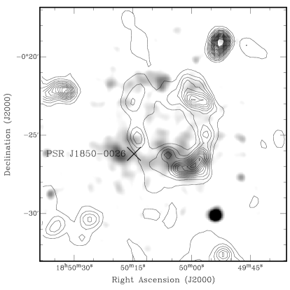
By considering a random sample of positions in this area of the sky, one can estimate the probability of a chance alignment between PSR J1850-0026 and SNR G32.45+0.1. We chose a large sample of randomly distributed sky positions with $-50^{\circ}<l<50^{\circ}$ and $|b|<1^{\circ}$ and searched for coincident positions in the catalogue of supernova remnants. At a separation of 2.5 arc minutes, the probability of a chance alignment is approximately $0.25\%$. Given that there are 218 known pulsars in this area of the sky, the expected number of chance alignments is $0.7$. If a reduced set of only the 28 known pulsars with ages less than 100 kyr are selected, then only $0.07$ chance alignments are expected.

Hydrogen absorption measurements suggest that the distance to the remnant is $17~{}\pm~{}11$ kpc Yamaguchi et al. (2004), which is compatible with the estimated distance to the pulsar of $11\pm 5$ kpc, calculated using the measured DM and the NE2001 Cordes & Lazio (2002) electron density model.

Reliable association of pulsars with supernova remnants is difficult, and it is impossible to completely rule out the possibility of a chance alignment. There are however several tests that can give a good indication that an association is likely. The most significant of these is a measurement of the proper motion of the pulsar. It would be expected that the pulsar would originate in the centre of the remnant, so that the proper motion should be directed away from this point. Measurement of proper motion usually requires several years of observation, and accurate measurements have been made on other similar pulsars Hobbs et al. (2004). Assuming that the pulsar was born in the supernova explosion, we can use the pulsar’s characteristic age (but see Kramer et al., 2003 for potential problems) and the projected distance of the pulsar from the centre of the explosion (from the distance estimates and the angular separation), we can estimate the velocity of the pulsar perpendicular to the line of sight. The distribution of pulsar velocities is well known Hobbs et al. (2005), and therefore if the computed velocity lies outside of the range of measured velocities then association is unlikely. Unfortunately there are large systematic errors in both the distance and the age measurements, such that the velocity measurement is highly uncertain. For PSR J1850--0026, the expected transverse velocity is approximately $140$ km/s for a nominal distance of 11 kpc, age of 68 kyr and a separation of 2.5 arc minutes. This velocity scales proportionally to changes in any of the three input parameters, although the computed value is well within the range of measured pulsar velocities. Given the above, it appears that there is a significant probability that PSR J1850--0026 is associated with SNR G32.45+0.1.

5 Statistical analysis

In order to determine if the new candidate selection techniques are selecting a statistically different set of pulsars, we compare our discoveries with those presented in Faulkner et al. (2004). We choose this sample of 142 pulsars because the survey parameters and processing code used were identical, thus the only difference is in the means of filtering the millions of candidates selected by the search algorithms. Unfortunately due to the fact that JReaper was designed to automatically detect and remove known pulsars from the results, it is only possible to compare the discovered pulsars, rather than all detected pulsars. An attempt to consider the effectiveness of JReaper at detecting pulsars is presented in Section 5.1.

The distribution of pulsar periods is split into two populations, one comprising millisecond pulsars and the other normal pulsars. The set of newly discovered pulsars contains no very short-period pulsars, i.e those with a spin period of less than 20 ms. Extrapolation of the expected number of short-period pulsars from the previous analysis suggests that the new results should contain $2.5\pm 1.6$ short-period pulsars. The small number of new pulsar discoveries make it difficult to determine if the absence of new discoveries of short-period pulsars is really significant.

Figure 5: Cumulative distribution plot of periods for two samples of pulsars, using a logarithmic scale.

Figure 6: Cumulative distribution plot of signal-to-noise ratios for two samples of pulsars, using a logarithmic scale.

Figure 7: Cumulative distribution plot of DMs for two samples of pulsars, using a logarithmic scale.

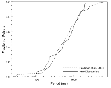
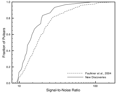
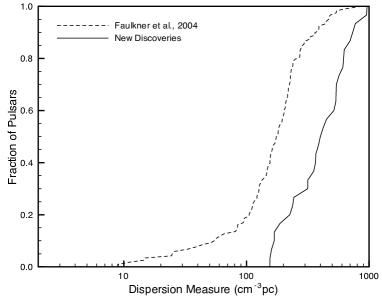
Figure 5 shows the cumulative distribution of the rotational periods of the two samples. A two-sample Kolmogorov-Smirnov test (KS test) determines that these samples are statistically indistinguishable. This implies that there are no difference in the period distributions of pulsars found by the two searches.

Figure 6 again shows a cumulative distribution plot, this time showing the signal-to-noise ratios for the detections in the two data sets. Although only significant at the 95% level, it appears that the new search methods may improve sensitivity to low signal-to-noise-ratio candidates. We can speculate that this difference may be due to the fact that brighter sources are more likely to have been detected in earlier, predominantly signal-to-noise-ratio based searches.

Figure 8: The DM and score values for a sample of pulsar candidates from the PMPS. The darker points show the discoveries presented here, the known pulsars and candidates that were selected for re-observation but were not confirmed. The lighter grey points are candidates produced by the search processing that were not selected for re-observation and are likely due to noise or interference. The vertical bands visible in the noise candidates are caused by the re-sampling of the data at higher DM values.

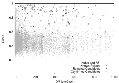
Figure 7 shows a similar plot, displaying the cumulative distribution of the DMs of the two samples. In this case it is clear that the distributions differ, and the KS test verifies that these distributions differ with a significance level of greater than $99\%$. The mean DM for the Faulkner et al. pulsars is 199 cm^-3pc, considerably lower than the mean value of 453 cm^-3pc in the new data set. Clearly it is important to determine if the new techniques are selecting against low-DM pulsars or if it is picking up high-DM pulsars that have previously been missed. Figure 8 indicates that the score of pulsars does not appear to be a function of the DM value, and although there are a greater number of false positives at lower DM values, the ratio of false positives (score $>$ 0.7) to number of candidates produced remains constant over the entire DM range. Therefore, at least in terms of the scoring algorithms, there appears to be no selection effect against low-DM pulsars.

It seems then that the pulsars presented in this work are from the same distribution of pulse periods as sampled in the earlier work, although we have tended to discover pulsars with a lower flux density and a greater DM.

It is also worth noting that the two new detections with the highest signal-to-noise ratio have periodicities of 99.7 ms and 500.3 ms, i.e. very close to the 10th and 2nd harmonics of 1 second, often a strong interference signal. It is probable therefore that these two sources were not detected in the original processing because they were close to interference signals and therefore ignored. This suggests that whilst the new techniques are best suited for detecting weaker pulsars in the data, they are also effective at distinguishing stronger pulsars from interference signals.

5.1 Effectiveness of JReaper as a search tool

To assess the effectiveness of a tool such as JReaper is difficult because the final choice of candidates to re-observe is still dependant on the user.

The most significant, and testable, enhancement provided by JReaper is the pulsar scoring system. A simple test of the score system’s effectiveness can be carried out by performing a blind search for known pulsars. This can be implemented by sorting all candidates by their score and determining how many pulsars are found per candidate searched. This can be compared to the same process, but sorting candidates by the more standard signal-to-noise ratio. The candidates were separated into three period ranges; less than 20ms, between 20ms and 500ms and greater than 500ms. The results of this analysis are presented in Figure 4.

Figure 9: These figures show the number of pulsars detected per candidate searched when analysing candidates ordered by signal-to-noise ratio or JReaper score, for candidates in three ranges of period.

This analysis clearly shows that for all period ranges the pulsar scoring system is effective at selecting pulsars from other candidates, when compared to the method based purely on the signal-to-noise ratio. Unfortunately the relative scarcity of millisecond pulsars makes the difference difficult to determine, although each pulsar is detected earlier when ordered by score than by signal-to-noise ratio. The most significant effect is for the period range greater than 500ms. This is most likely to be due to the fact that for longer periods there is an abundance of impulsive interference, which the scoring can easily distinguish from pulsar-like signals. In this region, to detect $90\%$ of the detectable known pulsars, one must search $\sim 4$ times fewer candidates compared to a ranking based simply on signal-to-noise ratio. For the 20-500ms region, this figure drops to $\sim 3$ times.

Clearly this blind search is not the most efficient means of searching for pulsars. One would need to individually inspect of the order of $10^{5}$ candidates to find $90\%$ of the $\sim 700$ known pulsars in the data. Whilst this may be possible, it would be more efficient to use the various JReaper plots to more intelligently select the candidates to view. The blind search does however illustrate the relative effectiveness of the scoring system over an approach based upon the signal-to-noise ratio.

6 Conclusion

Using new candidate selection techniques we discovered 28 pulsars that were initially missed in the analysis of the Parkes Multi-beam Pulsar Survey. Amongst these discoveries are an eccentric binary system and a young pulsar spatially coincident with a supernova remnant. Although the fractional increase in discoveries is relatively small, application of these new techniques comes with little cost. We believe that future search efforts will benefit from application of candidate selection methods as presented here, in addition to the established methods.

Acknowledgements

This research was partly funded by grants from the Science & Technology Facilities Council, UK. The Australia Telescope is funded by the Commonwealth of Australia for operation as a National Facility managed by the CSIRO. The authors would like to thank the following people for their contributions to observing at Parkes: M. Burgay, A. Noutsos, G.Hobbs, J. O’Brien, I. Stairs, A. Corongiu, M. Purver, R. Smits and C. Espinoza.

References

- Condon et al. (1998) Condon J. J., Cotton W. D., Greisen E. W., Yin Q. F., Perley R. A., Taylor G. B., Broderick J. J., 1998, AJ, 115, 1693
- Cordes & Lazio (2002) Cordes J. M., Lazio T. J. W., preprint (arXiv:astro-ph/0207156)
- Duda & Hart (1972) Duda R. O., Hart P. E., 1972, Comm. ACM, 15, 1
- Faulkner et al. (2004) Faulkner A. J. et al., 2004, MNRAS, 355, 147
- Green (2006) Green D. A., 2006, A catalogue of galactic supernova remnants (2006 april version), http://www.mrao.cam.ac.uk/surveys/snrs/
- Hobbs et al. (2004) Hobbs G. et al., 2004, MNRAS, 352, 1439
- Hobbs et al. (2005) Hobbs G., Lorimer D. R., Lyne A. G., Kramer M., 2005, MNRAS, 360, 974
- Hobbs et al. (2004) Hobbs G., Lyne A. G., Kramer M., Martin C. E., Jordan C., 2004, MNRAS, 353, 1311
- Hobbs et al. (2006) Hobbs G. B., Edwards R. T., Manchester R. N., 2006, MNRAS, 369, 655
- Hough (1960) Hough P. V. C., 1960, Us patent number 3069653: Method and means for recognising complex patterns
- Keith et al. (2008) Keith M. J., Kramer M., Lyne A. G., Eatough R. P., Stairs I. H., Possenti A., Camilo F., Manchester R. N., 2008, MNRAS, in press (arXiv:0811.2027)
- Kramer et al. (2003) Kramer M. et al., 2003, MNRAS, 342, 1299
- Kramer et al. (2006) Kramer M., Lyne A. G., O’Brien J. T., Jordan C. A., Lorimer D. R., 2006, Science, 312, 549
- Lorimer et al. (2006) Lorimer D. R. et al., 2006, MNRAS, 372, 777
- Lorimer & Kramer (2005) Lorimer D. R., Kramer M., 2005, Handbook of Pulsar Astronomy. Cambridge University Press
- Manchester et al. (2001) Manchester R. N. et al., 2001, MNRAS, 328, 17
- McLaughlin et al. (2006) McLaughlin M. A. et al., 2006, Nature, 439, 817
- Morris et al. (2002) Morris D. J. et al., 2002, MNRAS, 335, 275
- Taylor & Cordes (1993) Taylor J. H., Cordes J. M., 1993, ApJ, 411, 674
- Yamaguchi et al. (2004) Yamaguchi H., Ueno M., Koyama K., Bamba A., Yamauchi S., 2004, PASJ, 56, 1059