Existence and stability of stationary solutions to spatially extended autocatalytic and hypercyclic systems under global regulation and with nonlinear growth rates

Abstract

Analytical analysis of spatially extended autocatalytic and hypercyclic systems is presented. It is shown that spatially explicit systems in the form of reaction-diffusion equations with global regulation possess the same major qualitative features as the corresponding local models. In particular, using the introduced notion of the stability in the mean integral sense we prove the competitive exclusion principle for the autocatalytic system and the permanence for the hypercycle system. Existence and stability of stationary solutions are studied. For some parameter values it is proved that stable spatially non-uniform solutions appear.

Keywords:

Autocatalytic system, hypercycle, reaction-diffusion, non-uniform stationary solutions, stability

1 Introduction and background

In 1971 Manfred Eigen published a seminal paper on the evolution of error-prone self-replicating macromolecules [9]. His theory was expanded significantly later on, primarily in works of Eigen, Schuster and co-workers [10, 11, 12]. One of the principal findings was the existence of the error threshold, i.e., the critical mutation rate such that the equilibrium population of macromolecules (the quasispecies in the terminology of Eigen et al.) cannot provide conditions for evolution if the fidelity of copying falls below this critical level. This critical mutation rate depends on the length of macromolecules and hence puts limits on the amount of information that can be carried by a given macromolecule. To improve fidelity one needs longer sequences (e.g., a more efficient replicase), to have longer sequences one needs better fidelity, hence the chicken–egg problem. An easy and obvious solution to this problem is that the early primordial genomes must have consisted of independently replicating entities, which, generally speaking, would compete with each other (see, e.g., [21] and references therein).

If we consider a simple mathematical description of independent competing replicators then the usual differential equations for the growth take the following form:

$$\frac{\dot{v}_{i}}{v_{i}}=a_{i}v_{i}^{p}-f_{1}(t),\quad i=1,\ldots,n,$$ (1.1)

where $v_{i}=v_{i}(t)$ is the concentration of the $i$-th type of macromolecules, $a_{i}$ is the rate of replicating, $p>0$ is the degree of auto-catalysis, and $f_{1}(t)$ is the term which is necessary to keep the total concentration constant, this term depends only on $t$ and not on the index, $f_{1}(t)=\sum_{i=1}^{n}a_{i}v_{i}^{p}v_{i}$ in the present case; easy to see that this is equivalent to the condition $\sum_{i=1}^{n}v_{i}=1$. In the case if $p\neq 1$ we have system with non-linear growth rates, which model different coupling strength of the various components, for the discussion of such growth rates see, e.g., [23, 24]. Hereinbelow we consider mainly $p>0$ (or even, $p>1$) but remark that $p=0$ gives the exponential growth, $p=1$ gives the standard hyperbolic growth (autocatalysis), and for $p<0$ the parabolic growth occurs [27]. It is straightforward to show that for $p\geq 0$ only one replicator present at $t\to\infty$, the competition winds up in the competitive exclusion of all but one types, i.e., the genome composed of independently replicating entities is not vital.

Figure 1: The hypercycle [12]. Each macromolecule $(M_{i})$ helps to replicate another one, $M_{i+1}$, $M_{n}$ macromolecule promotes the replication of $M_{1}$ closing the loop; $a_{i},\,i=1,\ldots,n$ denote reaction rates.

To resolve this situation Eigen and Schuster [12] suggested a concept of the hypercycle, a group of self-replicating macromolecules that catalyze each other in a cyclic manner: the first type helps the second one, the second type helps the third, etc, and the last type helps the first one closing the loop (see Fig. 1). An analogue to system (1.1) can be written in the form

$$\frac{\dot{v}_{i}}{v_{i}}=a_{i}v_{i-1}^{p}-f_{2}(t),\quad i=1,\ldots,n,$$ (1.2)

where index $0$ coincides with $n$, $f_{2}(t)=\sum_{i=1}^{n}a_{i}v_{i-1}^{p}v_{i}$. For $p=1$ we obtain the standard hypercycle model [18]. It is known that (1.2) is permanent, i.e., all the concentrations are separated from zero, and hence different replicators coexist in this model. More exactly, for short hypercycles, $n=2,3,4$, the internal equilibrium is globally stable, for longer hypercycles, $n>4$, a globally stable limit cycle appears [17].

The problem with the hypercycle model (1.2) is its vulnerability to the invasion of parasites [22].

We remark that models (1.1) and (1.2) are systems of ordinary differential equation (ODEs), i.e., they are mean-field models. As a solution to the parasite invasion problem it was suggested that heterogeneous population structure can strengthen persistence of the system. One of the suggested solution was spatially explicit models [1, 3, 7], see also [2, 6] for reviews of the pertinent work. Two major approaches to spatially explicit models are reaction-diffusion equations and cellular automata models, and they both were considered in the cited works. Which was lacking, however, is an analytical treatment of the resulting systems, because in both cases the researchers have resorted to extensive numerical simulations. An only notable exception to our knowledge is [32], where some of the models with explicit space are analyzed analytically. An interest in cluster-like solutions of reaction-diffusion systems resulted in the analysis of spatially explicit hypercycle in infinite space [30, 31].

Note that models (1.1) and (1.2) are a special case of the general replicator equation [19], for which several approaches are known to incorporate an explicit spatial structure, albeit there is no universally accepted way of incorporating dispersal effects. The solution to the problem with equal diffusion rates is straightforward, in this case we, following ecological approach, can just add the Laplace operator to the right hand sides of (1.1) or (1.2). This was used, e.g., in the classical paper by Fisher [14] to model the effect of the spatial structure on the invasion properties of an advantageous gene; this approach later was generalized by Hadeler [16]. However, for the primordial world, it would be a too stringent an assumption to have all the diffusion coefficients equal. To overcome this difficulty, Vickers et al. introduced a special form of the population regulation to allow for different diffusion rates [5, 20, 29], now in the subject area of evolutionary game dynamics. In these works a nonlinear term is used that provides local regulation of the populations under question, although no particular biological mechanism is known that lets individuals adapt their per capita birth and death rates to local circumstances [13]. In our view, it is more natural to assume the global regulation of the populations, hence following along the lines of thought that brought to the models (1.1) and (1.2). Mathematically it means that we assume that the total populations satisfy the following condition

$$\sum_{i=1}^{n}\int_{\Omega}v_{i}(t,x)\,dx=1,$$

where $x\in\Omega$ is a spatial variable now. This approach was first used in [32]. Which is important here is that this approach allows to obtain some analytical insights of the systems [4].

In this text our goal is to present an analytical treatment of the models of prebiotic macromolecules with self- and hypercyclic catalysis with an explicit spatial structure and global population regulation in the form of reaction-diffusion equations.

2 The mathematical models

Let $\Omega$ be a bounded domain, $\Omega\subset\mathbb{R}^{m}$, $m=1,2,3$, with a piecewise-smooth boundary $\Gamma$. The spatially explicit analogue to (1.1) is given by the following reaction-diffusion system

$$\partial_{t}v_{i}=v_{i}(a_{i}v_{i}^{p}-f_{1}(t))+d_{i}\Delta v_{i},\quad i=1,\ldots,n,\quad t>0.$$ (2.1)

Here $v_{i}=v_{i}(x,t),\,x\in\Omega,t>0$, $\partial_{t}\equiv\frac{\partial}{\partial t}$, $\Delta$ is the Laplace operator, in the Cartesian coordinates $\Delta=\sum_{k=1}^{m}\frac{\partial^{2}}{\partial x_{i}^{2}}$. The initial conditions are $v_{i}(x,0)=\varphi_{i}(x)$, $p>0$ (although we note, that in each particular case we shall specify admissible values of $p$), and the form of $f_{1}(t)$ will be determined later.

A slight modification of (2.1) gives the hypercyclic system

$$\partial_{t}v_{i}=v_{i}(a_{i}v_{i-1}^{p}-f_{2}(t))+d_{i}\Delta v_{i},\quad i=1,\ldots,n,\quad t>0,$$ (2.2)

where $v_{0}\equiv v_{n}$.

In both problems (2.1) and (2.2) the functions $v_{i}(x,t)$ are assumed to be nonnegative, since they represent relative concentrations of different macromolecules.

It is natural to assume that we consider closed systems (see also [32]), i.e., we have the boundary conditions

$$\left.\frac{\partial v_{i}}{\partial\textbf{n}}\right|_{x\in\Gamma}=0,\quad i=1,\ldots,n,$$ (2.3)

where n is the normal vector to the boundary $\Gamma$.

It is assumed that the global regulation of the total concentration of macromolecules occurs in the system such that

$$\sum_{i=1}^{n}\int_{\Omega}v_{i}(x,t)\,dx=1$$ (2.4)

for any time moment $t$. This condition is an analogous condition for the total concentration of replicators in the finite-dimensional case [18]. From the boundary condition (2.3) and the integral invariant (2.4) the expressions for the functions $f_{1}(t)$ and $f_{2}(t)$ follow:

$$f_{1}(t)=\sum_{i=1}^{n}\int_{\Omega}a_{i}v_{i}^{p+1}(x,t)\,dx$$ (2.5)

and

$$f_{2}(t)=\sum_{i=1}^{n}\int_{\Omega}a_{i}v_{i-1}^{p}(x,t)v_{i}(x,t)\,dx.$$ (2.6)

Finally we have a mixed problem for a system of semilinear parabolic equations with the integral invariant (2.4) and functionals (2.5) and (2.6).

Suppose that for any fixed $x\in\Omega$ each function $v_{i}(x,t)$ is differentiable with respect to variable $t$, and belongs to the space $H_{p+1}^{1}(\Omega)$ as the function of $x$ for any fixed $t>0$. Here $H_{p+1}^{1}$ is the space of functions with the norm

$$\|u(x)\|_{H_{p+1}^{1}}=\left[\int_{\Omega}|u(x)|^{p+1}\,dx\right]^{\frac{1}{p+1}}+\left[\int_{\Omega}\sum_{k=1}^{m}\left|\frac{\partial u}{\partial x_{k}}\right|^{2}\,dx\right]^{\frac{1}{{2}}}.$$

Note that if $p\geq 1$ then $H_{p+1}^{1}(\Omega)\subseteq H_{2}^{1}(\Omega)$, where $H_{2}^{1}(\Omega)$ is the Sobolev space of square-integrable functions for which their first partial derivatives are also square-integrable [25].

Without loss of generality we shall assume further that volume of the domain $\Omega$ is equal 1: $|\Omega|=1$.

Our main goal is to analyze existence and stability of the steady state solutions to (2.1) and (2.2). The steady state solutions are given by the solutions to the following elliptic problems:

$$d_{i}\Delta u_{i}+u_{i}(a_{i}u_{i}^{p}-\bar{f}_{1})=0,\quad i=1,\ldots,n,$$ (2.7)

and

$$d_{i}\Delta u_{i}+u_{i}(a_{i}u_{i-1}^{p}-\bar{f}_{2})=0,\quad i=1,\ldots,n,\quad u_{0}\equiv u_{n},$$ (2.8)

with the boundary conditions $\partial_{\textbf{n}}u_{i}=0$ on $\Gamma$; $u_{i}(x)\in H_{p+1}^{1}(\Omega)$. The integral invariant (2.4) now reads

$$\sum_{i=1}^{n}\int_{\Omega}u_{i}(x)\,dx=1,$$ (2.9)

the values of $\bar{f}_{1}$ and $\bar{f}_{2}$ are constant:

$$\bar{f}_{1}=\sum_{i=1}^{n}\int_{\Omega}a_{i}u_{i}^{p+1}(x)\,dx$$ (2.10)

and

$$\bar{f}_{2}=\sum_{i=1}^{n}\int_{\Omega}a_{i}u_{i-1}^{p}(x)u_{i}(x)\,dx.$$ (2.11)

If it is assumed that $d_{1}=d_{2}=\ldots=d_{n}=0$ then the equilibrium points of (1.1) and (1.2) coincide with the steady state solutions to (2.1) and (2.2). These solutions are spatially homogeneous. The converse is also true: the spatially homogeneous equilibria of systems (2.1) and (2.2) are fixed points of the dynamical systems (1.1) and (1.2) respectively.

The coordinates of these spatially homogeneous solutions are straightforward to write down. Let $\beta_{i}=(a_{i})^{-\frac{1}{p}}$ and consider the sum $\beta=\sum\beta_{i}$, where the index of summation is determined later. All spatially homogeneous solutions to (2.7) are given by

$$\begin{split}P_{1}&=\frac{1}{\beta}(\beta_{1},\,\beta_{2},\ldots,\beta_{n}),\\ Q_{j}&=\frac{1}{\beta}(\beta_{1},\ldots,\beta_{j-1},0,\beta_{j+1},\ldots,\beta_{n}),\\ Q_{jk}&=\frac{1}{\beta}(\beta_{1},\ldots,\beta_{j-1},0,\beta_{j+1},\ldots,\ldots,\beta_{k-1},0,\beta_{k+1},\ldots,\beta_{n}),\\ &\ldots\end{split}$$

ending with the vertices $R_{i}=(0,\ldots,0,1,0,\ldots,0)$ (unity at the $i$-th place) of the simplex $\sum_{i=1}^{n}u_{i}=1,\,u_{i}\geq 0$; for each steady state $\beta$ in obtained by summing through all non-zero elements in the vector.

The spatially homogeneous stationary solution to (2.8) is given by

$$P_{2}=\frac{1}{\beta}(\beta_{2},\,\beta_{3},\ldots,\beta_{n},\,\beta_{1}).$$

3 Stability of spatially homogeneous equilibria

Let $u^{0}=(u_{1}^{0},\ldots,u_{n}^{0})$ be a spatially homogeneous solution to system (2.1). In the usual way we assume that the Cauchy data are perturbed

$$\varphi_{i}(x)=u_{i}^{0}+w_{i}(x),\quad i=1,\ldots,n.$$

Here $w_{i}(x)\in H_{p+1}^{1}(\Omega)$. Inasmuch as we have

$$\sum_{i=1}^{n}u_{i}^{0}=1,$$

then from (2.4) it follows that

$$\sum_{i=1}^{n}\int_{\Omega}w_{i}(x)\,dx=0.$$ (3.1)

Consider the following eigenvalue problem

$$\Delta\psi(x)+\lambda\psi(x)=0,\quad x\in\Omega,\quad\partial_{\textbf{n}}\psi(x)|_{x\in\Gamma}=0.$$ (3.2)

The system of eigenfunctions of this problem $\psi_{0}(x)=1$, $\{\psi_{i}(x)\}_{i=1}^{\infty}$ forms a complete system in the Sobolev space $H_{1}^{1}(\Omega)$ [25] such that

$$\langle\psi_{i}(x),\psi_{j}(x)\rangle=\int_{\Omega}\psi_{i}(x)\psi_{j}(x)\,dx=\delta_{ij},$$

where $\delta_{ij}$ is the Kronecker symbol. The corresponding eigenvalues satisfy the condition

$$0=\lambda_{0}<\lambda_{1}\leq\lambda_{2}\leq\ldots\leq\lambda_{i}\leq\ldots,\quad\lim_{i\to\infty}\lambda_{i}=\infty.$$

Hence for $p\geq 1$ we assume that $w_{i}(x)$ can be represented as

$$w_{i}(x)=\sum_{j=0}^{\infty}c_{j}^{i}\phi_{j}(x),\quad i=1,\ldots,n,$$ (3.3)

where $c_{j}^{i}$ are constant.

Denote $H_{\delta}$ the set of functions $w(x)\in H_{1}^{1}(\Omega)$ such that $\|w\|_{H_{1}^{1}}\leq\delta$, where $\delta>0$.

Theorem 3.1.

For $p\geq 1$ all spatially homogeneous stationary solutions to (2.1) are unstable with respect to any perturbation from the set $H_{\delta}$ if

$$0<\frac{d_{i}}{a_{i}}<\frac{p}{\lambda_{1}},\quad i=1,\ldots,n.$$ (3.4)

The solutions $R_{i}=(0,\ldots,0,1,0,\ldots,0)$, $i=1,\ldots,n$ are stable when

$$\frac{d_{i}}{a_{i}}>\frac{p}{\lambda_{1}}\,.$$ (3.5)

Here $\lambda_{1}$ is the first non-zero eigenvalue of the problem (3.2).

Proof.

Let $W(x,t)=(W_{1}(x,t),\ldots,W_{n}(x,t))$ be a vector-function belonging to $H_{\delta}$ for any fixed $t$. Using (3.1) and (3.2) we can seek the solution to (2.1) in the following form:

$$v_{i}(x,t)=u_{i}^{0}+W_{i}(x,t),\quad W_{i}(x,t)=\sum_{j=0}^{n}c_{j}^{i}(t)\psi_{j}(x).$$ (3.6)

Substituting (3.6) into (2.1) and retaining in the usual way only linear terms with respect to $W_{i}$ we obtain the following equations:

$$\partial_{t}W_{i}=(p+1)a_{i}(u_{i}^{0})^{p}W_{i}-\bar{f}_{1}W_{i}+d_{i}\Delta W_{i},\quad W_{i}(x,0)=\varphi_{i}(x)\in H_{\delta},\quad\partial_{\textbf{n}}W_{i}=0\mbox{ on }\Gamma.$$ (3.7)

Consider first the case $u^{0}=P_{1}$. Direct calculations show that $\bar{f}_{1}=\beta^{-p}$.

Multiplying equations (3.7) one after another by the functions $\psi_{j}$ and integrating with respect to $x\in\Omega$ we obtain the following system of ordinary differential equations:

$$\frac{dc_{j}^{i}(t)}{dt}=c_{j}^{i}(t)(a_{i}p\beta^{-p}-d_{i}\lambda_{j}),\quad i=1,\ldots,n,\quad j=0,1,2,\ldots$$ (3.8)

For $j=0$ one has

$$c_{0}^{i}(t)=c_{0}^{i}(0)\exp(a_{i}p\beta^{-p}t),$$

therefore, $c_{0}^{i}(t)\to\infty$ as $t\to\infty$, which implies that $P_{1}$ is unstable.

Using the same approach it is straightforward to show that $Q_{j},\,Q_{jk},\ldots$ are also unstable.

Now we deal with $R_{i}$. First note that from (2.9) it follows that

$$\sum_{i=1}^{n}c_{0}^{i}(t)=0.$$ (3.9)

For $R_{i}$ we have

$$\frac{dc_{j}^{i}(t)}{dt}=-c_{j}^{i}(t)(a_{i}+d_{i}\lambda_{j}),\quad\mbox{for }j\neq i$$

and

$$\frac{dc_{j}^{i}(t)}{dt}=c_{j}^{i}(t)(a_{i}-d_{i}\lambda_{j}),\quad\mbox{for }j=i.$$

Therefore, for $j\neq i$, $c_{i}^{j}(t)\to 0$ when $t\to\infty$. Taking into account (3.9) we obtain that $c_{0}^{i}(t)\to 0$. If $i=j$ and (3.4) holds then $c_{j}^{i}(t)\to\infty$, if (3.5) holds then $c_{j}^{i}(t)\to 0$, which proves the theorem. ∎

Theorem 3.2.

If $p\geq 1$ then spatially homogeneous stationary solution $P_{2}$ to system (2.2) is unstable with respect to any perturbations from the set $H_{\delta}$ when

$$\prod_{i=1}^{n}\frac{d_{i}}{a_{i}}<\left(\frac{p}{\beta^{p}\lambda_{1}}\right)^{n}.$$ (3.10)

Proof.

As before we will look for a solution to (2.2) in the form (3.6). After substituting (3.6) into (2.2), multiplying by $\psi_{j}$ and integrating, we obtain the following system of ordinary differential equations for $c_{j}^{i}(t)$:

$$\frac{dc_{j}^{i}(t)}{dt}=\frac{p}{\beta^{p}}\frac{a_{i}}{a_{i+1}}c_{j}^{i-1}(t)-d_{i}\lambda_{j}c_{j}^{i}(t),\quad i=1,\ldots n,\,n+1\equiv 1,\,0\equiv n,\quad j=0,1,2,\ldots$$ (3.11)

Applying the Routh–Hurwitz criterion we obtain that the solutions to (3.11) go to $\infty$ if (3.10) holds, which implies instability of $P_{2}$. ∎

Remark 3.1.

Inverse inequality to (3.10) provides stability of $P_{2}$ only in the cases $n=2,3,4$. Actually, for $j=0$ we have that (3.11) takes the form

$$\frac{dc_{0}^{i}(t)}{dt}=\frac{p}{\beta^{p}}\frac{a_{i}}{a_{i+1}}c_{0}^{i-1}(t),\quad i=1,\ldots,n.$$

All eigenvalues can be easily evaluated because the corresponding matrix is circular:

$$\mu_{j}=\frac{p}{\beta^{p}}\rho_{j},\quad j=0,\ldots,n-1,$$

where $\rho_{j}$ is the $j$-th root of the equation $\rho^{n}=1$. The eigenvector $(1,1,\ldots,1)$ does not satisfy (3.9), therefore we exclude it from the consideration. When $n=2,3$ all eigenvalues have negative real part, in the case $n=4$ $P_{2}$ also will be stable [18]. For $n\geq 5$ there is at least one eigenvalue with positive real part, which proves the claim that $P_{2}$ is unstable when $n\geq 5$.

4 Existence of spatially nonuniform stationary solutions to systems (2.1) and (2.2) in one-dimensional case

Here we will prove that when the space is one dimensional, $\Omega=[0,1],\,\Delta=\partial_{x}$, the models (2.1) and (2.2) possess non-uniform stationary solutions under some additional conditions. The boundary conditions now take the form $\partial_{x}v_{i}(0,t)=\partial_{x}v_{i}(1,t)=0$.

Theorem 4.1.

For $0<p\leq 2$ a spatially non-uniform stationary solution to (2.1) exists if the following inequality holds

$$\sum_{i=1}^{n}\left(\frac{d_{i}}{a_{i}}\right)^{\frac{1}{p}}<\left(\frac{p}{\pi^{2}}\right)^{\frac{1}{p}}.$$ (4.1)

Proof.

We start the proof noting that the dependence of the concentrations $u_{i}(x)$ in (2.7) on other concentrations and their total regulations occur only through the integral invariant (2.10), which does not depend on $x$. Therefore we can assume without loss of generality that each $u_{i}$ depends on its own variable $x_{i}\in[0,1]$. Hence we rewrite (2.9) and (2.10) in the form

$$\begin{split}&\sum_{i=1}^{n}\int_{\Omega}u_{i}(x_{i})\,dx_{i}=1,\\ \bar{f}_{1}&=\sum_{i=1}^{n}\int_{\Omega}a_{i}u_{i}^{p+1}(x_{i})\,dx_{i}.\end{split}$$ (4.2)

Each equation of system (2.7) can be put in the following form:

$$\begin{split}\frac{du_{i}}{dx_{i}}&=V_{i},\\ \frac{dV_{i}}{dx_{i}}&=\frac{1}{d_{i}}(\bar{f}_{1}-a_{i}u_{i}^{p})u_{i}.\end{split}$$ (4.3)

System (4.3) is a Hamiltonian system for any $i=1,\ldots,n$, in which $x_{i}$ is considered as a “time” variable, with the Hamiltonian

$$H_{i}=\frac{V_{i}^{2}}{2}+\frac{1}{d_{i}}\left(\frac{d_{i}}{p+2}u_{i}^{p+2}-\frac{\bar{f}_{1}}{2}u_{i}^{2}\right).$$

The phase orbits of (4.3) can be found from the standard formula

$$V_{i}=\pm\sqrt{2(H_{i}^{0}-U_{i})},$$

where

$$H_{i}^{0} =\frac{V_{i}^{2}(x_{i}^{0})}{2}+\frac{1}{d_{i}}\left(\frac{d_{i}}{p+2}u_{i}^{p+2}(x_{i}^{0})-\frac{\bar{f}_{1}}{2}u_{i}^{2}(x_{i}^{0})\right),$$

$$U_{i} =\frac{1}{d_{i}}\left(\frac{d_{i}}{p+2}u_{i}^{p+2}-\frac{\bar{f}_{1}}{2}u_{i}^{2}\right).$$

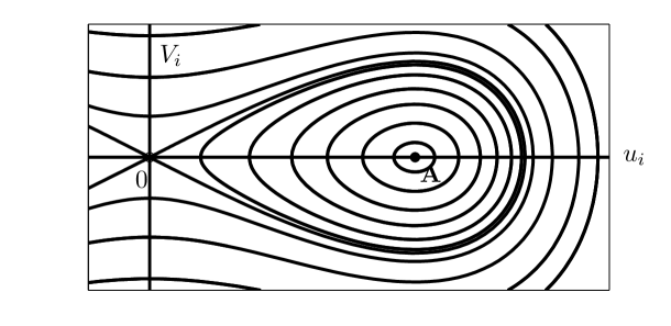
Figure 2: The phase portrait of system (4.3). The closed curves surrounding $\bf{A}$ correspond to the candidates for spatially non-homogeneous stationary solutions to (2.1)

From the form of the phase orbits (see Fig. 2) it immediately follows that there exist orbits that satisfy the condition

$$V_{i}(x_{i}^{1})=V_{i}(x_{i}^{2})=0,\quad x_{i}^{1}\neq x_{i}^{2}.$$

These orbits represent closed curves surrounding the center point $\textbf{A}=\left(\left({\bar{f}_{1}}{a_{i}^{-1}}\right)^{\frac{1}{p}},\,0\right)$ in Fig. 2. Different diffusion coefficients correspond to the motion along the phase orbits with different velocities.

To prove the theorem we need to show that there exist two values $x_{i}^{1}$ and $x_{i}^{2}$ such that $|x_{i}^{1}-x_{i}^{2}|$=1, for $i=2,\ldots,n$, and corresponding solutions to (2.7) satisfy the first condition in (4.2).

The solutions to system (2.7) can be found in the explicit parametric form [26]:

$$\begin{split}u_{i}(x_{i})&=\left[\frac{p+2}{2a_{i}}\bar{f}_{1}\right]^{\frac{1}{p}}\tau,\quad\tau\geq 0,\\ x_{i}&=\sqrt{\frac{d_{i}}{\bar{f}_{1}}}\int_{\tau_{0}}^{\tau}\frac{dt}{\sqrt{P_{i}(t)}}+c_{i}^{2},\quad P_{i}(t)=c_{i}^{1}+t^{2}-t^{p+2},\\ u_{i}(x_{i})&=-\left[\frac{p+2}{2a_{i}}\bar{f}_{1}\right]^{\frac{1}{p}}\tau,\quad\tau\leq 0,\\ x_{i}&=\sqrt{\frac{d_{i}}{\bar{f}_{1}}}\int_{\tau_{0}}^{\tau}\frac{dt}{\sqrt{Q_{i}(t)}}+c_{i}^{2},\quad Q_{i}(t)=c_{i}^{1}+t^{2}+t^{p+2}.\end{split}$$ (4.4)

To proceed we need the following lemma (the proof is given in the Appendix).

Lemma 4.1.

The equation $P_{i}(t)=c_{i}^{1}+t^{2}-t^{p+2}=0$ has two real positive roots $0<\tau_{i}^{1}<\tau_{i}^{2}$ for all values

$$c_{i}^{1}\in\left(-\left[\frac{2}{2+p}\right]^{\frac{2}{p}+1},\,0\right).$$ (4.5)

Moreover,

$$\tau_{i}^{1}\in\left(0,\,\left[\frac{2}{2+p}\right]^{\frac{2}{p}}\right),\quad\tau_{i}^{2}\in\left(\left[\frac{2}{2+p}\right]^{\frac{2}{p}},\,1\right).$$ (4.6)

An analogous lemma holds for $Q_{i}(t)$.

Now we return to the parametric representation (4.4). Consider the first derivative of the functions $u_{i}$:

$$\frac{du_{i}}{dx_{i}}=\frac{du_{i}}{d\tau}\frac{d\tau}{dx_{i}}=\left[\frac{p+2}{2a_{i}}\bar{f}_{1}\right]^{\frac{1}{p}}\sqrt{\frac{d_{i}}{\bar{f}_{1}}}\sqrt{P_{i}(t)}.$$

This expression vanishes at the points $\tau_{i}^{1}$ and $\tau_{i}^{2}$. Using (4.4) for $x_{i}=0$ and $x_{i}=1$, we obtain

$$\begin{split}x_{i}=0&\longrightarrow\quad\sqrt{\frac{d_{i}}{\bar{f}_{1}}}\int_{\tau_{0}}^{\tau_{i}^{1}}\frac{dt}{\sqrt{P_{i}(t)}}+c_{i}^{2}=0\\ x_{i}=1&\longrightarrow\quad\sqrt{\frac{d_{i}}{\bar{f}_{1}}}\int_{\tau_{0}}^{\tau_{i}^{2}}\frac{dt}{\sqrt{P_{i}(t)}}+c_{i}^{2}=1.\end{split}$$ (4.7)

Letting $\tau_{0}=\tau_{i}^{1}$ we obtain that $c_{i}^{2}=0$. We will use the following notation:

$$I_{i}^{1}=\int_{\tau_{i}^{1}}^{\tau_{i}^{2}}\frac{dt}{\sqrt{P_{i}(t)}}=\sqrt{\frac{\bar{f}_{1}}{d_{i}}}.$$ (4.8)

Remark that these integrals will exist because the roots of $P_{i}(t)$ are simple when $c_{i}^{1}$ satisfy (4.5). The formula (4.8) establishes the connection between the values of the constant $c_{i}^{1}$ and values of the diffusion coefficient $d_{i}$, which determines the velocity of motion of phase points. The latter implies that (4.8) guaranteers that the motion from the initial point $(u_{i}^{1},0)$ to the final point $(u_{i}^{2},0)$ occurs during the unit time.

Now we are going to prove that the solution (4.4) satisfies the first condition in (4.2):

$$\sum_{i=1}^{n}\int_{0}^{1}u_{i}(x_{i})\,dx_{i}=\left[\frac{p+2}{2}\right]^{\frac{1}{p}}\sum_{i=1}^{n}\left[\frac{\bar{f}_{1}}{a_{i}}\right]^{\frac{1}{p}}\sqrt{\frac{d_{i}}{\bar{f}_{1}}}\int_{\tau_{i}^{1}}^{\tau_{i}^{2}}\frac{tdt}{\sqrt{P_{i}(t)}}=1.$$ (4.9)

From (4.9) it follows that

$$\left[\frac{p+2}{2}\right]^{\frac{1}{p}}\sum_{i=1}^{n}\left[\frac{\bar{f}_{1}}{a_{i}}\right]^{\frac{1}{p}}\sqrt{\frac{d_{i}}{\bar{f}_{1}}}\int_{\tau_{i}^{1}}^{\tau_{i}^{2}}\frac{(p+2)t^{p+1}/2-tdt}{\sqrt{P_{i}(t)}}=0.$$

Indeed, we have

$$\begin{split}&\int_{\tau_{i}^{1}}^{\tau_{i}^{2}}\frac{(p+2)t^{p+1}/2-tdt}{\sqrt{P_{i}(t)}}=\frac{1}{2}\int_{\tau_{i}^{1}}^{\tau_{i}^{2}}\frac{d(t^{p+2}-t^{2})}{\sqrt{P_{i}(t)}}=\\ &=-\frac{1}{2}\int_{\tau_{i}^{1}}^{\tau_{i}^{2}}\frac{d(P_{i}(t))}{\sqrt{P_{i}(t)}}=-\left(\sqrt{P_{i}(\tau_{i}^{2})}-\sqrt{P_{i}(\tau_{i}^{1})}\right)=0.\end{split}$$

Using (4.8) to find $\bar{f}_{1}$ and substituting this expression into (4.9) we obtain

$$\left[\frac{p+2}{2}\right]^{\frac{1}{p}}\sum_{i=1}^{n}\left[\frac{d_{i}}{a_{i}}\right]^{\frac{1}{p}}\left(I_{i}^{1}\right)^{\frac{2}{p}-1}\left(I_{i}^{2}\right)=1,$$ (4.10)

where

$$I_{i}^{1}=\int_{\tau_{i}^{1}}^{\tau_{i}^{2}}\frac{dt}{\sqrt{P_{i}(t)}},\quad I_{i}^{2}=\int_{\tau_{i}^{1}}^{\tau_{i}^{2}}\frac{tdt}{\sqrt{P_{i}(t)}}.$$

To conclude the proof we need the following lemma, the proof of which is given in the Appendix

Lemma 4.2.

If $0<p\leq 2$ then the following inequality holds:

$$I(c_{i}^{1})=(I_{i}^{1})^{\frac{2}{p}-1}\left[\frac{p+2}{2}\right]^{\frac{1}{p}}I_{i}^{2}>\left[\frac{\pi^{2}}{p}\right]^{\frac{1}{p}}.$$ (4.11)

Applying the result of Lemma 4.2 to (4.10) we obtain that if (4.1) holds then there exists a spatially non-uniform stationary solution to (2.1). ∎

Remark 4.1.

From the symmetry of the system, the time needed to get from the point $(u_{i}^{1},0)$ to the point $(u_{i}^{2},0)$ is the same as the time needed to get from $(u_{i}^{2},0)$ to $(u_{i}^{1},0)$, and the speed of movement is inversely proportional to $\sqrt{d_{i}}$. Therefore, reducing these values twice we guaranteer that spatially non-uniform stationary solution exists, which corresponds to the full cycle in the phase plane; reducing 4 times we obtain the solution which corresponds to the movement of the phase point along the cycle two times, and so on. Hence system (2.1) has non-uniform stationary solutions that correspond to movement along the cycles in Fig. 2 arbitrary number of times (see Fig. 3).

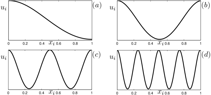
Figure 3: Spatially non-uniform stationary solutions to (2.1) which satisfy the conditions $|x_{i}^{1}-x_{i}^{2}|=1$, and the boundary conditions. $(a)$ A solution that corresponds to the movement along half the cycle in Fig. 2; $(b)$ full cycle; $(c)$ two full cycles; $(d)$ four full cycles. Changing $d_{i}$ and hence the velocity of the movement along the phase curves we can always obtain solutions with arbitrary number of full cycles

Remark 4.2.

We introduce the following parameter

$$d=\sum_{i=1}^{n}\left(\frac{d_{i}}{a_{i}}\right)^{\frac{1}{p}}.$$ (4.12)

Theorem 4.1 can be restated as follows: If

$$d<\mu=(p\pi^{-2})^{\frac{1}{p}}$$

then there exists a spatially non-uniform stationary solution to (2.1). On the other hand, if $d>\mu$ we obtain from Theorem 3.1 that $R_{i}$ are stable. Therefore we can consider $d$ as a bifurcation parameter. As this parameter decreases spatially uniform stationary solutions become unstable, and spatially non-uniform solutions appear in the system according to the standard Turing bifurcation scenario.

Now we consider the case of the spatially explicit hypercycle (2.2).

Theorem 4.2.

Suppose that (4.1) holds. If the parameters of problem (2.2) can be represented by one-parameter perturbation

$$d_{i}=d_{0}+\varepsilon l_{i},\quad a_{i}=a_{0}+\varepsilon m_{i},\quad m_{i},\,l_{i}\mbox{ are constant,}\quad\varepsilon>0,$$

where $\varepsilon$ is a small parameter, then there exist spatially non-uniform stationary solutions to system (2.2).

Proof.

System (2.2) can be rewritten in the following form:

$$d_{i}u_{i}^{\prime\prime}+u_{i}(a_{i}u_{i}-\bar{f}_{1})=u_{i}a_{i}(u_{i}-u_{i-1})+(\bar{f}_{1}-\bar{f}_{2})u_{i},\quad i=1,\ldots,n.$$ (4.13)

If $\varepsilon=0$ then we have that $\bar{f}_{1}=\bar{f}_{2}$ and

$$d_{0}u_{i}^{\prime\prime}+u_{i}(a_{0}u_{i}-\bar{f}_{1})=0,$$ (4.14)

which is a particular case of the autocatalytic system (2.7). According to Theorem 4.1 system (4.14) possesses spatially non-uniform stationary solutions. Using the presentation (4.4) it can be shown that the right hand side of (4.13) is of the order of $\varepsilon$, i.e., can be rewritten in the form

$$d_{i}u_{i}^{\prime\prime}+u_{i}(a_{i}u_{i}-\bar{f}_{1})=\varepsilon\Psi_{i}(x),\quad i=1,\ldots,n.$$ (4.15)

where $\Psi_{i}(x)$ are bounded functions. This implies that system (4.15) is a perturbation of the Hamiltonian system (4.14). According to the general theory [15] stable and unstable manifolds of the perturbed orbits will be close to the corresponding manifolds of the unperturbed system. Therefore for $d<\mu$ for each non-uniform stationary solution of (2.1) there exists spatially non-uniform stationary solution to (2.2). ∎

Remark 4.3.

If we assume that the inverse to inequality (3.10) holds, then it can be rewritten in the form

$$\sum_{i=1}^{n}\left[\frac{d_{i}}{a_{i}}\right]^{\frac{1}{p}}>\frac{p^{\frac{1}{p}}}{\pi^{\frac{2}{p}}}.$$

Indeed, we can rewrite inverse to (3.10) in the form

$$\left[\prod_{i=1}^{n}d_{i}\right]^{\frac{1}{pn}}>\frac{p^{\frac{1}{p}}}{\beta\pi^{\frac{2}{p}}}.$$

Using the properties of arithmetic and geometric means we obtain

$$\beta=\sum_{i=1}^{n}\frac{1}{(a_{i})^{\frac{1}{p}}}\leq n\left[\prod_{i=1}^{n}\frac{1}{(a_{i})^{\frac{1}{p}}}\right]^{\frac{1}{n}}.$$

From the previous it follows that

$$n\left[\prod_{i=1}^{n}d_{i}\right]^{\frac{1}{pn}}\left[\prod_{i=1}^{n}\frac{1}{(a_{i})^{\frac{1}{p}}}\right]^{\frac{1}{n}}=n\left[\prod_{i=1}^{n}\left[\frac{d_{i}}{a_{i}}\right]^{\frac{1}{p}}\right]^{\frac{1}{n}}>\frac{p^{\frac{1}{p}}}{\pi^{\frac{2}{p}}}.$$

Once again using the inequality between arithmetic and geometric means we obtain

$$n\left[\prod_{i=1}^{n}\left[\frac{d_{i}}{a_{i}}\right]^{\frac{1}{p}}\right]^{\frac{1}{n}}\leq\sum_{i=1}^{n}\left[\frac{d_{i}}{a_{i}}\right]^{\frac{1}{p}},$$

which proves the desired result.

In words, we showed in this remark that if the inverse to (3.10) holds, then the inverse to (4.1) is true, which means that if the spatially homogeneous solution to hypercycle system is stable there are no spatially non-homogeneous solutions.

Example 4.1.

It is possible to obtain an explicit solution to (2.8) in the special case when $n=4$, $d_{1}=d_{3},\,d_{2}=d_{4},\,a_{i}=a,\,i=1,2,3,4$. First, we rewrite (2.11) in the form

$$\bar{f}_{2}=\int_{0}^{1}\langle Au,u\rangle dx,\quad u=(u_{1},u_{2},u_{3},u_{4})^{\prime}.$$

The expression $\langle u,v\rangle$ denotes the standard scalar product in $\mathbb{R}^{4}$, ^′ is the transformation. Matrix $A$ is circular and has eigenvalues $\lambda_{1}=a,\,\lambda_{3}=-a,\,\lambda_{2}=\lambda_{4}=0$. Consider the orthogonal transformation that reduces $A$ to its canonical form:

$$T=\left(\begin{array}[]{cccc}1/2&\sqrt{2}/2&-1/2&0\\ 1/2&0&1/2&-\sqrt{2}/2\\ 1/2&\sqrt{2}/2&-1/2&0\\ 1/2&0&1/2&-\sqrt{2}/2\\ \end{array}\right).$$

Summing all equations in the hypercyclic system we have

$$\langle u_{xx},D\rangle=\bar{f}_{2}\langle u,\textbf{1}\rangle-\langle Au,u\rangle,$$

where $D$ is the diffusion vector, $D=(d_{1},d_{2},d_{1},d_{2})$, $\textbf{1}=(1,1,1,1)$. Let $u(x)=Tv(x)$, $v=(v_{1},v_{2},v_{3},v_{4})$. It follows that

$$\langle v_{xx},T^{\prime}D\rangle=\bar{f}_{2}\langle v,T^{\prime}\textbf{1}\rangle-\langle T^{\prime}ATV,v\rangle.$$

Since $\langle T^{\prime}ATV,v\rangle=k(v_{1}^{2}-v_{3}^{2})$, the last equation takes the form

$$(d_{1}+d_{2})(v_{1})_{xx}=2\bar{f}_{2}v_{1}-k(v_{1}-v_{3}).$$

Suppose that $u_{1}+u_{3}=u_{2}+u_{4}$. Then we have that $v_{3}=0$ and the function $w(x)=u_{1}+u_{2}$, satisfies the differential equation

$$(d_{1}+d_{2})w_{xx}=2\bar{f}_{2}w-aw^{2},$$

whose explicit solution can be found using (4.4).

Remark 4.4.

As in the case of system (2.1) parameter $d$ can be considered as a bifurcation parameter for (2.2).

5 Asymptotic behavior of the spatially explicit autocatalytic and hypercyclic systems

Consider the local system of autocatalytic reaction (1.1) in the form

$$\begin{split}\frac{dw_{i}}{dt}&=w_{i}(a_{i}w_{i}^{p}-f_{1}^{loc}(t)),\quad f_{1}^{loc}(t)=\sum_{i=1}^{n}a_{i}w_{i}^{p+1},\quad t>s,\\ w_{i}(s)&=\xi_{i},\quad i=1,\ldots,n,\quad\sum_{i=1}^{n}w_{i}=1.\end{split}$$ (5.1)

For the following we need

Definition 5.1.

We shall say that the initial conditions for system (2.1) and system (5.1) are concerted if

$$\xi_{i}=\bar{\varphi}_{i}=\int_{\Omega}\varphi_{i}(x)dx.$$ (5.2)

Let us assume that the initial conditions for systems (2.1) and (5.1) are concerted. On integrating system (2.1) with respect to $x$ and using the equality $\int_{\Omega}\Delta v(x)dx=\int_{\Gamma}\partial_{\textbf{n}}vds=0$ we obtain

$$\frac{d\bar{v}_{i}}{dt}=a_{i}\int_{\Omega}v_{i}^{p+1}(x,t)dx-\bar{v}_{i}(t)f_{1}^{loc}(t),\quad t>s,\quad\bar{v}_{i}(s)=\bar{\varphi}_{i}=\xi_{i},\quad i=1,\ldots,n,$$

where

$$\bar{v}_{i}(t)=\int_{\Omega}v_{i}(x,t)dx.$$

Since $|\Omega|=1$ we have

$$\int_{\Omega}v_{i}^{p+1}(x,t)dx\geq\left(\int_{\Omega}v_{i}(x,t)\,dx\right)^{p+1}=\bar{v}_{i}^{p+1}(t),$$

and, consequently,

$$\frac{d\bar{v}_{i}}{dt}\geq\bar{v}_{i}^{p+1}(t)-\bar{v}_{i}(t)f_{1}^{loc}(t),\quad t>s,\quad\bar{v}_{i}(s)=\bar{\varphi}_{i}=\xi_{i},\quad i=1,\ldots,n,$$ (5.3)

Lemma 5.1.

Let the initial conditions for systems (2.1) and (5.1) be concerted. Then

$$\beta^{-p}\leq f_{1}^{loc}(t)\leq f_{1}(t),$$ (5.4)

where $\beta=\sum_{i=1}^{n}a_{i}^{-\frac{1}{p}}$.

Proof.

First, we prove the left inequality in (5.4). Using (2.4) and Hölder’s inequality we have

$$1=\left(\sum_{i=1}^{n}w_{i}(t)\right)^{p+1}\leq\left[\sum_{i=1}^{n}\frac{1}{a_{i}^{p}}\right]^{p}\sum_{i=1}^{n}a_{i}w_{i}^{p+1}=\beta^{p}f_{1}^{loc}(t).$$

To prove the right inequality in (5.4) we assume that there exists $s\geq 0$ that $f_{1}(s)<f_{1}^{loc}(s)$. Since the functions $f_{1}(t)$ and $f_{1}^{loc}$ are continuous, there exists neighborhood $U_{\delta}=\{t\colon 0\leq t-s<\delta\}$ from which $f_{1}(t)<f_{1}^{loc}(t)$ follows. Then from (5.3) it follows that

$$\frac{d\bar{v}_{i}}{dt}\geq\bar{v}_{i}^{p+1}(t)-\bar{v}_{i}(t)f_{1}(t),\quad t\in U_{\delta},\quad i=1,\ldots,n.$$ (5.5)

Due to the fact that the initial conditions of (2.1) and (5.1) are concerted, then from the comparison theorem [28] we obtain

$$\bar{v}_{i}(t)>w_{i}(t),\quad t\in U_{\delta},\quad i=1,\ldots,n,$$ (5.6)

where $w_{i}(t)$ are the solutions to (5.1). From the other hand we should have $\sum_{i=1}^{n}\bar{v}_{i}(t)=\sum_{i=1}^{n}w_{i}(t)=1$; we obtain a contradiction.

∎

Theorem 5.1.

Let $p\geq 1$. Then for almost all initial conditions $\varphi_{i}(x),\,\sum_{i=1}^{n}\int_{\Omega}\varphi_{i}(x)dx=1$ there exists an index $j$, $1\leq j\leq n$ (which depends on $\varphi_{i}(x)$) such that ${v}_{i}(x,t)\to 0$ for all $i\neq j$ in the space $L_{p+1}$, and $\int_{\Omega}{v}_{j}(x,t)\to 1$ when $t\to\infty$.

Proof.

We have $p\geq 1$, and hence $H_{p+1}^{1}\subseteq H_{2}^{1}$. The eigenfunctions $\psi_{s},\,s=0,1,2,\ldots$ of the problem (3.2) form a complete system in $H_{2}^{1}$. Let us represent

$$\varphi_{i}(x)=\bar{c}_{i}^{0}+z_{i}(x),\quad z_{i}(x)=\sum_{s=1}^{\infty}\bar{c}_{i}^{s}\psi_{s}(x).$$

Let $w_{i}(t)$ be the solutions to (5.1) and let the initial conditions for systems (2.1) and (5.1) be concerted. We will look for a solution to (2.1) in the form

$$\begin{split}v_{i}(x,t)&=w_{i}(t)+z_{i}(x,t),\quad z_{i}(x,t)=\sum_{s=0}^{\infty}c_{i}^{s}(t)\psi_{s}(x),\\ w_{i}(0)&=c_{i}^{0},\quad c_{i}^{m}(0)=\bar{c}_{i}^{m},\quad m=1,2,\ldots\end{split}$$ (5.7)

Inserting (5.7) into (2.1) we obtain

$$\frac{dw_{i}(t)}{dt}+\frac{\partial z_{i}(x,t)}{\partial t}=a_{i}v_{i}^{p+1}(x,t)-f_{1}(t)(w_{i}(t)+z_{i}(x,t))+d_{i}\frac{\partial^{2}z_{i}(x,t)}{\partial x^{2}}.$$

Integrating the last equation with respect to $x$ and noting $\int_{\Omega}\psi_{s}(x)dx=0$ give

$$\frac{dw_{i}(t)}{dt}=a_{i}\int_{\Omega}v_{i}^{p+1}(x,t)dx-f_{1}(t)w_{i}(t).$$

Using the fact that $w_{i}(t)$ are the solutions to (5.1) we obtain

$$a_{i}\int_{\Omega}v_{i}^{p+1}(x,t)dx=(f_{1}(t)-f_{1}^{loc}(t))w_{i}(t)+a_{i}w_{i}^{p+1}(t).$$ (5.8)

It is known that solutions to (5.1) have a property of multistability. It means that all the vertexes of the simplex are stable, and the choice of initial conditions determines to which vertex the system evolves. In other words, for almost all initial conditions $\xi_{i}$ the system (5.1) ends up in $R_{j}$, for which all the coordinates excluding $j$ are zero ($w_{i}(t)\to 0$ when $t\to\infty$ for all $i\neq j$, and $w_{j}(t)\to 1$). Hence, from (5.8) the theorem follows. ∎

Remark 5.1.

Theorem (5.1) answers a natural question which spatially non-uniform stationary solution of (2.1) survives in the evolutionary process. To answer it we need to consider two systems (2.1) and (5.1) with concerted initial conditions. As was mentioned system (5.1) possesses the property of multistability; each vertex of the simplex has its own basin of attraction. If we denote these basins as $D_{1},\ldots,D_{n}$, then the number of the basin, to which the initial conditions of (5.1) belong, determines which spatially non-uniform solution will dominate the evolution. Note that for the dominant solution

$$\int_{\Omega}v(x,t)dx\to 1\mbox{ for }t\to\infty.$$ (5.9)

Another point here is that the explicit space structure in the system with global regulation (2.1) does not provide the conditions for surviving more than one type of prebiotic replicators, $v_{i}(x,t)\to 0$ in $L_{p+1}$ for all $i\neq j$.

Corollary 5.1.

Almost all spatially non-uniform stationary solutions of the problem (2.1) are unstable.

Proof.

Consider (2.1) with the initial conditions

$$v_{i}(x,s)=u_{i}(x)+\beta_{i}(x),\quad i=1,\ldots,n,$$

where $u_{i}(x)$ are spatially non-uniform stationary solutions to (2.1), and $\beta_{i}(x)\in H_{\delta}$. From Theorem 5.1 it follows that there exists a positive integer $j$ (which depends on the initial conditions) such that $v_{i}(x,t)\to 0$ in space $L_{p+1}$ for $i\neq j$. Therefore only one set of stationary solutions can be stable. ∎

Remark 5.2.

It is possible to obtain sufficient conditions for stability of the non-uniform stationary solution $u_{j}(x)>0,\,\int_{\Omega}u_{j}(x)dx=1$. Unfortunately, applying this condition requires additional serious analysis.

Indeed, we can look for a solution to (2.1) in the form

$$v_{j}(x,t)=u_{j}(t)+z_{j}(x,t),\quad v_{i}(x,t)=z_{i}(x,t),\,i\neq j.$$

Putting these solutions into (2.1) and retaining only linear terms we obtain

$$\begin{split}\partial_{t}z_{j}(x,t)&=a_{j}(p+1)[u_{j}^{p}(x)z_{j}(x,t)-\langle u_{j}^{p}(x),z_{j}(x,t)\rangle]-a_{j}z_{j}(x,t)\langle u_{j}^{p+1}(x),1\rangle+d_{i}\Delta z_{j}(x,t),\\ \partial_{t}z_{i}(x,t)&=-a_{i}z_{i}(x,t)\langle u_{i}^{p+1}(x),1\rangle+d_{i}\Delta z_{i}(x,t),\quad i\neq j,\end{split}$$

with the initial conditions $z_{i}(x,s)=u_{i}(x)+\beta_{i}(x)$. Here $\langle u(x),v(x)\rangle$ denotes the usual scalar product in $L_{2}(\Omega)$. This implies that all $z_{i}(x,t)\to 0$ for $i\neq j$ when $t\to\infty$. On the other hand we have

$$\begin{split}\frac{1}{2}\frac{d}{dt}\int_{\Omega}z_{j}^{2}(x,t)dx&=a_{j}(p+1)[\langle u_{j}^{p}(x),z_{j}^{2}(x,t)\rangle-\langle u_{j}(x),z_{j}(x,t)\rangle\langle u_{j}^{p}(x),z_{j}(x,t)\rangle]\\ &{}-a_{j}\langle z_{j}(x,t),z_{j}(x,t)\rangle\langle u_{j}^{p+1},1\rangle+d_{i}\langle\Delta z_{j}(x,t),z_{j}(x,t)\rangle.\end{split}$$ (5.10)

Substituting the following

$$z_{j}(x,t)=z_{j}^{0}(t)+\sum_{s=1}^{\infty}z_{j}^{s}(t)\psi_{s}(x)$$

into (5.10) and using the fact that

$$\langle\Delta z_{j}(x,t),z_{j}(x,t)\rangle=-\sum_{s=1}^{\infty}\lambda_{s}(z_{j}^{s}(t))^{2}$$

we obtain that all the terms in (5.10) except for the terms in the square brackets are negative. The terms in the square brackets have the following form

$$\alpha=(p+1)\sum_{m=1}^{\infty}\sum_{s=1}^{\infty}a_{j}z_{j}^{m}(t)z_{j}^{s}(t)(\langle u_{j}^{p}(x),\psi_{m}(x)\psi_{s}(x)\rangle-\langle u_{j}(x),\psi_{m}(x)\rangle\langle u_{j}^{p}(x),\psi_{s}(x)\rangle),$$

from which we obtain a sufficient condition for stability of the solution $u_{j}(x)>0$ in the form

$$\alpha<\sum_{m=1}^{\infty}(z_{j}^{m}(t))^{2}(\lambda_{m}+a_{j}\bar{u}_{j}^{p}).$$

The last formula should be checked only for small $m$ because $\lambda_{m}\to\infty$.

The result of Lemma 5.1 can be extended to the case of hypercycle reaction.

Lemma 5.2.

Let the initial conditions of system (2.2) and system

$$\begin{split}\frac{dw_{i}}{dt}&=w_{i}(a_{i}w_{i-1}^{p}-f_{2}^{loc}(t)),\quad f_{2}^{loc}(t)=\sum_{i=1}^{n}a_{i}w_{i}w_{i-1}^{p},\quad t>0,\\ w_{i}(0)&=\xi_{i},\quad i=1,\ldots,n,\quad\sum_{i=1}^{n}w_{i}=1\end{split}$$ (5.11)

be concerted. Then

$$f_{2}^{loc}(t)\leq f_{2}(t).$$ (5.12)

Proof.

We have

$$\int_{\Omega}\frac{\Delta v_{i}}{v_{i}}\,dx=\int_{\Gamma}\frac{\partial v_{i}}{\partial\textbf{n}}\frac{1}{v_{i}}\,ds+\int_{\Omega}|\nabla_{x}\ln v_{i}|^{2}dx\geq 0,$$

and

$$\int_{\Omega}v^{p}_{i-1}(x,t)dx\geq\left(\int_{\Omega}v_{i-1}(x,t)dx\right)^{p}=\bar{v}_{i-1}^{p}.$$

Therefore

$$\int_{\Omega}\frac{\partial}{\partial t}\ln v_{i}\,dx\geq a_{i}\bar{v}^{p}_{i-1}(t)-f_{2}(t).$$

Since the initial conditions of (2.2) and (5.11) are concerted, then, as in the case of Theorem (5.1) we can represent $v_{i}(x,t)$ as the sum $v_{i}(x,t)=w_{i}(t)+z_{i}(x,t)$, where $z_{i}(x,t)$ are given by (5.7), and note that $w_{i}(0)=\bar{v}_{i}(0)$ for any $i$.

From the last inequality it follows that

$$\int_{\Omega}\frac{\partial}{\partial t}\ln v_{i}\,dx=\frac{d}{dt}w_{i}(t)\geq a_{i}\bar{v}_{i-1}^{p}-f_{2}(t).$$

Since $\bar{v}_{i}(0)=w_{i}(0)$ then, using (5.11) we obtain (5.12). ∎

Using the last lemma we can extend the results of permanence of hypercycle system with $p=1$ to the spatially explicit case [18]. We remind that permanence means that solutions to system (5.11) with the initial conditions $w_{i}(0)=\xi_{i}>0$ do not vanish, i.e.,

$$1>w_{i}(t)>\delta>0,\quad t>0.$$

Corollary 5.2.

Let $p=1$ and let the initial conditions of systems (2.2) and (5.11) be concerted, and

$$\bar{\varphi_{i}}=\xi_{i}=w_{i}(0)>0,\quad\sum\xi_{i}=1.$$

Then the solutions to system (2.2) do not vanish in $L_{2}$ space.

Proof.

Let a solution $v_{i}(x,t)$ to (2.2) vanish for some $i$, i.e.,

$$\|v_{i}(x,t)\|_{L_{2}}\to 0,\quad t\to\infty.$$

Using the reasoning along the lines of Theorem 5.1, we obtain

$$a_{i}\int_{\Omega}v_{i}(x,t)v_{i-1}(x,t)\,dx=(f_{2}(t)-f_{2}^{loc}(t))w_{i}(t)+a_{i}w_{i}(t)w_{i-1}(t).$$

Using Lemma 5.2 we hence have

$$\int_{\Omega}v_{i}(x,t)v_{i-1}(x,t)\,dx\geq w_{i}(t)w_{i-1}(t).$$

The last and the Cauchy inequalities yield

$$\|v_{i}(x,t)\|_{L_{2}}\|v_{i-1}(x,t)\|_{L_{2}}\geq w_{i}(t)w_{i-1}.$$

From the fact $\|v_{i}(x,t)\|_{L_{2}}\to 0$ it follows that either $w_{i}$ or $w_{i-1}$ tend to zero, which contradicts to the permanence of the hypercycle system (5.11). This completes the proof. ∎

Similar to Remark 5.2 we can obtain sufficient conditions for stability of the spatially nonhomogeneous stationary solutions for the hypercycle system (2.2). However, the utility of such conditions is questionable because we hardly can expect that we will be able to check these conditions analytically.

It is possible to study the stability of spatially nonhomogeneous solutions in somewhat weaker sense.

Definition 5.2.

We shall say that spatially non-uniform stationary solution $u(x)=(u_{1}(x),\ldots,u_{n}(x))$ to system (2.1) or (2.2) is stable in the sense of the mean integral value if for any $\varepsilon>0$ there exists $\delta>0$ such that for the initial conditions

$$|\bar{\varphi}_{i}-\bar{u}_{i}|<\delta,$$

it follows that

$$|\bar{v}_{i}-\bar{u}_{i}|<\varepsilon,$$

for any $i$ and $t>0$, where, as before, $v_{i}(x,t)$ are the solutions of (2.1) or (2.2),

$$\bar{v}_{i}=\int_{\Omega}v_{i}(x,t)dx,\quad\bar{\varphi}_{i}=\int_{\Omega}\varphi_{i}(x)dx,\quad\bar{u}_{i}=\int_{\Omega}u_{i}(x)dx.$$

It is clear that the stability in the mean integral sense is weaker than the stability in the usual sense (Lyapunov stability). For example, consider functions $g(x,t)\in H_{2}^{1},\,x\in[0,1]$

$$g(x,t)=c_{0}(t)+\sum_{s=1}^{\infty}c_{k}(t)\cos k\pi x.$$

Let us suppose that $c_{0}(t)\to 0$ when $t\to\infty$. Then $\bar{g}(t)\to 0$ whereas $\|g(x,t)\|^{2}_{H_{2}^{1}}=\sum_{s=1}^{\infty}c_{k}^{2}(t)(1+k^{2}\pi^{2})$ does not necessarily tend to zero.

Corollary 5.3.

Let us suppose that the following inequalities hold for any $i=1,\ldots,n$:

$$\frac{d_{i}}{a_{i}}<\frac{p}{\lambda_{1}}\,.$$ (5.13)

Then all spatially non-uniform stationary solutions to (2.1) of the form

$$U^{j}(x)=(0,\ldots,0,u_{j}(x),0,\ldots,0)$$

are stable in the mean integral sense.

Proof.

From Theorem 3.1 it follows that $R_{j}$ are unstable when (5.13) holds. Consider the solution $U^{j}(x)$ for which $\bar{u}_{j}=1$. From the other hand from Theorem (5.1) follows (5.9), which completes the proof. ∎

Now we switch to the hypercycle system (2.2) with explicit spatial structure and global regulation. After integrating (2.2) with respect to spatial variable, we obtain

$$\frac{\bar{v}_{i}(t)}{dt}=a_{i}\langle v_{i-1}^{p},v_{i}\rangle-f_{2}(t)\bar{v}_{i}(t),\quad 0<t,\quad v_{i}(0)=\bar{\varphi}_{i},$$ (5.14)

where the meaning of the function $\bar{g}$ as before, in the mean integral sense.

Let us introduce new functions

$$v_{i}(x,t)=\frac{w_{i}(x,t)}{(a_{i})^{\frac{1}{p}}}\Theta,\quad i=1,\ldots,n,\quad\Theta=\int_{\Omega}\sum_{j=1}^{n}(a_{j})^{\frac{1}{p}}v_{j}(x,t)dx.$$ (5.15)

For the new variables

$$\sum_{j=1}^{n}\int_{\Omega}w_{j}(x,t)dx=1.$$ (5.16)

Note that in the new variables the stationary point $P_{2}$ has the coordinates $(1/n,1/n,\ldots,1/n)$.

Lemma 5.3.

In the new variables (5.15) the dynamical system (5.14) has the following form:

$$\begin{split}\frac{d\bar{w}_{i}(t)}{dt}&=\Theta^{p}(t)(\langle w_{i-1}^{p},w_{i}\rangle-f_{2}(t)\bar{w}_{i}(t)),\\ f_{2}(t)&=\sum_{j=1}^{n}\int_{\Omega}w_{j}(x,t)w_{j-1}^{p}(x,t)dx.\end{split}$$ (5.17)

Proof.

Using (5.15), (2.2) and the boundary conditions we obtain

$$\begin{split}\frac{d\Theta}{dt}&=\sum_{j=1}^{n}\int_{\Omega}(a_{j}v_{j}v_{j-1}^{p}-f_{2}(t)v_{j}+d_{j}\Delta v_{j})(a_{j+1})^{\frac{1}{p}}dx\\ &=\Theta^{p+1}\sum_{j=1}^{n}\int_{\Omega}w_{j}w_{j-1}^{p}dx-f_{2}(t)\Theta\sum_{j=1}^{n}\int_{\Omega}w_{j}dx\end{split}$$

Using (5.16) we obtain

$$\frac{d\Theta}{dt}=\Theta^{p+1}\sum_{j=1}^{n}\int_{\Omega}w_{j}w_{j-1}^{p}dx-f_{2}(t)\Theta.$$ (5.18)

Equality (5.15) yields

$$\frac{d\bar{v}_{i}}{dt}=\frac{\dot{\bar{w}}_{i}\Theta+\bar{w}_{i}\dot{\Theta}}{(k_{i+1})^{\frac{1}{p}}}\,.$$ (5.19)

From the other hand (5.15) implies

$$\frac{d\bar{v}_{i}}{dt}=\frac{\Theta^{p+1}\langle w_{i},w_{i-1}^{p}\rangle-\Theta\bar{w}_{i}f_{2}(t)}{(k_{i+1})^{\frac{1}{p}}}\,.$$ (5.20)

Putting together (5.18),(5.19) and (5.20) completes the proof. ∎

Consider the spatially uniform stationary solution $P_{2}$ to (2.2). It is also an equilibrium of (5.14).

Theorem 5.2.

Let $u(x)=(u_{1}(x),\ldots,u_{n}(x))$ be a spatially non-uniform stationary solution to (2.2) such that $\bar{u}=P_{2}$, where $P_{2}$ is the homogeneous stationary solution of (2.2). Then $u(x)$ is stable in the sense of the mean integral value.

Proof.

Consider system (5.14). Due to Lemma 5.3 this system is topologically equivalent to system (5.17), which has the steady state $P_{0}=(1/n,\ldots,1/n)$. Let us introduce the following Laypunov function

$$V(\bar{w}_{1},\ldots,\bar{w}_{n})=-\ln(\bar{w}_{1}\bar{w}_{2}\ldots\bar{w}_{n})-n\ln n.$$

It is easy to see that $V(P_{0})=0$ and $V(\bar{w}_{1},\ldots,\bar{w}_{n})>0$ in a neighborhood $Z_{\delta}$ of $P_{0}$, where

$$Z_{\delta}=\left\{\bar{w}_{i},i=1,\dots,n\,\,:\,\,\sum_{j=1}^{n}\bar{w}_{j}=1,\quad\sum_{j=1}^{n}|\bar{w}_{j}-\frac{1}{n}|\leq\delta\right\}.$$

Using (5.14) yields

$$\begin{split}\dot{V}&=-\sum_{i=1}^{n}\frac{\dot{\bar{w}}_{i}}{\bar{w}_{i}}=\\ &=-\Theta^{p}\sum_{i=1}^{n}\left[\frac{\langle w_{i},w_{i-1}^{p}\rangle}{\bar{w}_{i}}-f_{2}(t)\right]=\\ &=-\Theta^{p}\sum_{i=1}^{n}\langle w_{i},w_{i-1}^{p}\rangle(\frac{1}{\bar{w}_{i}}-n).\end{split}$$

Denote $\mu$ the following

$$\mu=\min_{1\leq i\leq n}\left\{\inf_{t}\langle w_{i},w_{i-1}^{p}\rangle\right\}.$$

The functions $w_{i}(x,t)$ are nonnegative for all $i$, therefore we obtain

$$\dot{V}\leq-\Theta^{p}\mu\left(\sum_{i=1}^{n}\frac{1}{\bar{w}_{i}}-n^{2}\right).$$

We also have $\sum_{i=1}^{n}\frac{1}{\bar{w}_{i}}\geq\frac{n}{\sqrt[n]{\prod_{i=1}^{n}\bar{w}_{i}}}$. Since $\sum_{i=1}^{n}\bar{w}_{i}=1,\,\bar{w}_{i}\geq 0$, the function $\prod_{i=1}^{n}\bar{w}_{i}$ reaches its maximum at the point $P_{0}=(1/n,\ldots,1/n)$, and this implies that

$$\frac{n}{\sqrt[n]{\prod_{i=1}^{n}\bar{w}_{i}}}\geq n^{2}$$

which means that $\dot{V}\leq 0$. Invoking the arguments of the topological equivalence of (5.14) and (5.17) completes the proof. ∎

6 Conclusion

In this paper we studied the existence and stability of stationary solutions to autocatalytic and hypercyclic systems (2.1) and (2.2) with nonlinear growth rates and explicit spatial structure. It is well known that the mean field models (e.g., models described by ODE systems) are often show different behavior from the models where the spatial structure is taken into consideration (more on this [8]). In particular, it is widely acknowledged that the evolution and survival of altruistic traits can be mediated by spatial heterogeneity. Macromolecules that catalyze the production of other macromolecules are obviously altruists, and in this note we tried to answer the question whether the particular form of spatial regulation (namely, global regulation [4, 32]) can promote the coexistence of different types of macromolecules in the prebiotic world (within a hydrothermally formed system of continuous iron-sulfide compartments [21]). The analysis presented in [4, 32] is significantly extended to the cases of nonlinear growth rates, arbitrary fitness and diffusion coefficients.

The major conclusion is as follows: the mathematical models with spatial structure and global regulation show in general very similar qualitative features to those of local models. Two basic properties, namely the competitive exclusion for autocatalytic systems and the permanence for the hypercyclic systems, are shown to hold for spatially explicit systems. Numerical calculations illustrate these conclusions in Figs. 4 and 5 (the details on the numerical scheme used in the calculations are given in [4]).

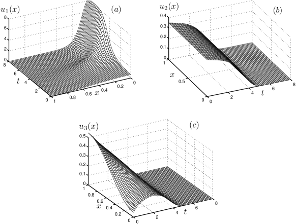
Figure 4: The competitive exclusion for autocatalytic growth. Numerical solutions to autocatalytic system (2.1). $n=3,\,d_{1}=0.02,\,d_{2}=0.05,\,d_{3}=0.08,\,p=1,\,a_{1}=a_{2}=a_{3}=1$. The initial conditions are $u_{1}(x,0)=0.35+0.3\cos\pi x,\,u_{2}(x,0)=0.35,\,u_{3}(x,0)=0.3-0.25\cos\pi x$. Note that the orientation of the axis is different for $(a)$ and $(b),\,(c)$. Only one type, $u_{1}$, survives. The asymptotic state is a spatially non-uniform stationary solution. The details of the numerical computations are given in [4]

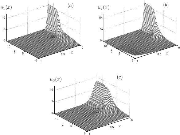
Figure 5: The permanence for the hypercycle system. Numerical solutions to hypercyclic system (2.2). $n=3,\,d_{1}=0.001,\,d_{2}=0.002,\,d_{3}=0.003,\,p=1,\,a_{1}=a_{2}=a_{3}=1$. The initial conditions are $u_{1}(x,0)=0.35+0.15\cos\pi x,\,u_{2}(x,0)=0.357,\,u_{3}(x,0)=0.338-0.3\cos\pi x$. The asymptotic state is spatially non-uniform stationary solutions. The details of the numerical computations are given in [4]

More precisely, for sufficiently large diffusion coefficients the spatially uniform stationary solutions to (2.1) and (2.2) have the same character as in the local models (1.1) and (1.2). For such diffusion coefficients the asymptotic behavior of the local and distributed models coincides. If, on the other hand, the inequality (4.1) holds and the nonlinear growth rates satisfy the condition $0<p\leq 2$ then new, spatially non-uniform solutions appear; for small diffusion coefficients these spatially heterogeneous solutions can correspond to the multiple cycles on the phase plane of the corresponding Hamiltonian system (Fig. 3). In the case of autocatalytic system these solution can be stable only if all but one asymptotic state are zero. In the case of the hypercyclic system we prove that these spatially heterogeneous solutions can be stable in the sense of the mean integral value. The examples of the asymptotic states for a hypercyclic systems found numerically are shown in Fig. 6. These non-uniform stationary solutions can be considered as the means of the hypercycle system to withstand the parasite invasion [22] (the analysis of models with parasites and with $p>2$ is the subject of the ongoing work).

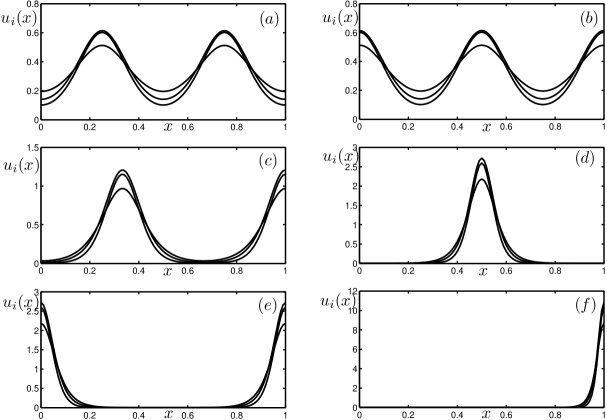
Figure 6: Asymptotic spatially heterogeneous states of the hypercycle system (2.8) found numerically. $n=3,\,d_{1}=0.001,\,d_{2}=0.002,\,d_{3}=0.003,\,p=1,\,a_{1}=a_{2}=a_{3}=1$. Note that case $(f)$ corresponds to the simulation shown in Fig. 5.

Appendix A Appendix

Proof of Lemma 4.1.

Consider the function $g(t)=t^{2}-t^{p+2},\,p>0$. This function has two roots $\tau_{1}=0$ and $\tau_{2}=1$, and attains its maximum at $t^{*}=\left[\frac{2}{2+p}\right]^{\frac{2}{p}}$, which is $g(t^{*})=\left[\frac{2}{2+p}\right]^{\frac{2}{p}+1}$. Function $P_{i}(t)$ can be obtained from $g(t)$ by shifting the latter. Therefore, when (4.5) holds, $P_{i}(t)$ has two positive roots that are situated in the interval (4.6). ∎

Proof of Lemma 4.2.

To simplify notations we drop indexes where it is possible. We need to prove that for

$$P(\tau,c)=c+\tau^{2}-\tau^{p+2}$$

and

$$I_{1}(c)=\int_{\tau_{1}}^{\tau_{2}}\frac{d\tau}{\sqrt{P(\tau,c)}},\quad I_{2}(c)=\int_{\tau_{1}}^{\tau_{2}}\frac{\tau\,d\tau}{\sqrt{P(\tau,c)}},$$ (A.1)

where

$$\tau_{1}\in(0,\tau_{0}),\quad\tau_{2}\in(\tau_{0},1),\quad\tau_{0}=\left[\frac{2}{2+p}\right]^{\frac{1}{p}},\quad P(\tau_{1},c)=0,\quad P(\tau_{2},c)=0,\quad P^{\prime}_{\tau}(\tau_{0},c)=0,$$

we have that

$$I(c)=\frac{1}{\tau_{0}}(I_{1}(c))^{\frac{2}{p}-1}I_{2}(c)\geq\left[\frac{\pi^{2}}{p}\right]^{\frac{1}{p}}$$ (A.2)

for $0<p\leq 2$.

For $p=2$ direct calculations show that $I_{2}(c)=\frac{\pi}{2},\,I(c)=\frac{\pi}{\sqrt{2}}$, hence we assume that $0<p<2$. Using Hölder’s inequality yields

$$(I_{1})^{\frac{2}{p}-1}I_{2}=\left[(I_{1})^{1-\frac{p}{2}}(I_{2})^{\frac{p}{2}}\right]^{\frac{2}{p}}\geq(I_{3})^{\frac{p}{2}},$$

where

$$I_{3}(c)=\int_{\tau_{1}}^{\tau_{2}}\left(\frac{1}{\sqrt{P(\tau,c)}}\right)^{1-\frac{p}{2}}\left(\frac{\tau}{\sqrt{P(\tau,c)}}\right)^{\frac{p}{2}}\,d\tau=\int_{\tau_{1}}^{\tau_{2}}\frac{\tau^{\frac{p}{2}}}{\sqrt{P(\tau,c)}}\,d\tau$$

Next we will the following change of the variables:

$$\tau^{\frac{p+2}{2}}=t,\quad\tau_{1}^{\frac{p+2}{2}}=t_{1},\quad\tau_{2}^{\frac{p+2}{2}}=t_{2},\quad\frac{4}{p+2}=q,\quad Q(t,c)=c+Q_{0}(t),\quad Q_{0}(t)=t^{q}-t^{2},\quad 1<q<2,$$

from which $Q(t_{1},c)=Q(t_{2},c)=0$, and hence $c=-Q_{0}(t_{1})=-Q_{0}(t_{2})$.

Out integral takes the form

$$I_{3}(c)=\frac{q}{2}\int_{t_{1}}^{t_{2}}\frac{1}{\sqrt{Q(t,c)}}\,dt,$$

$$t_{1}\in(0,t_{0}),\quad t_{2}\in(t_{0},1),\quad t_{0}=\left(\frac{q}{2}\right)^{\frac{1}{2-q}},\quad Q_{0}^{\prime}(t_{0})=0.$$

Function $Q(t,c)$ does not exceed its Hermite interpolation polynomial $H_{3}$, which is build using the values at $H_{3}(t_{1})=H_{3}(t_{2})=H_{3}^{\prime}(t_{0})=0,\,H_{3}(t_{0})=Q(t_{0},c)$. This follows from non-negativity of the reminder term of interpolation

$$Q(t,c)-H_{3}(t)=\frac{Q_{0}^{(4)}(\xi)}{24}(t-t_{0})^{2}(t-t_{1})(t-t_{2}),$$

and the fact that $Q_{0}^{(4)}(\xi)>0$ when $t_{1}<\xi<t_{2}$. Therefore, we have

$$I_{3}(c)>\frac{q}{2}\int_{t_{1}}^{t_{2}}\frac{1}{\sqrt{H_{3}(t)}}\,dt,$$

where

$$H_{3}(t)=Q(t_{0},c)\left(1-\frac{(t-t_{0})(2t_{0}-t_{1}-t_{2})}{(t_{0}-t_{1})(t_{0}-t_{2})}\right)\frac{(t-t_{1})(t-t_{2})}{(t_{0}-t_{1})(t_{0}-t_{2})}.$$

Making the change of the variable in the integral

$$t=\frac{t_{1}+t_{2}}{2}+\frac{t_{2}-t_{1}}{2}\sin\varphi,$$

we obtain

$$\int_{t_{1}}^{t_{2}}\frac{1}{\sqrt{H_{3}(t)}}\,dt=\sqrt{\frac{(t_{0}-t_{1})(t_{2}-t_{0})}{Q(t_{0},c)}}I_{4}(c),$$

where

$$I_{4}(c)=\int_{-\pi/2}^{\pi/2}\frac{d\varphi}{\sqrt{1-\frac{((t_{1}+t_{2})/2-t_{0}+(t_{2}-t_{1})/2\sin\varphi)(2t_{0}-t_{1}-t_{2})}{(t_{0}-t_{1})(t_{0}-t_{2})}}}.$$

Since the graph of any convex function lays above any tangent line, then we have

$$\frac{1}{\sqrt{c_{1}x+c_{2}}}\geq\frac{1}{\sqrt{c_{2}}}\left(1-\frac{c_{1}x}{2c_{2}}\right)$$

for any $x$. Using the last inequality we can estimate $I_{4}$ as

$$I_{4}>\int_{-\pi/2}^{\pi/2}\frac{1}{\sqrt{c_{2}}}\left(1-\frac{c_{1}\sin\varphi}{2c_{2}}\right)\,d\varphi=\frac{\pi}{\sqrt{c_{2}}}=\frac{\pi}{\sqrt{1-\frac{(2t_{0}-t_{1}-t_{2})^{2}}{2(t_{0}-t_{1})(t_{2}-t_{0})}}}>\pi.$$

Using the last estimate and returning to $I_{3}$ we obtain that

$$I_{3}(c)>\frac{q\pi}{2}\sqrt{\frac{(t_{0}-t_{1})(t_{2}-t_{0})}{Q(t_{0},c)}}=\frac{q\pi}{2}\sqrt[4]{g(t_{1})g(t_{2})},$$

where

$$g(t)=\frac{(t-t_{0})^{2}}{Q_{0}(t_{0})-Q_{0}(t)}\,.$$

With the help of the Taylor formula the denominator in $g(t)$ can be presented in the following form:

$$Q_{0}(t_{0})-Q_{0}(t)=-Q_{0}^{\prime\prime}(t_{0})(t-t_{0})^{2}/2-Q_{0}^{\prime\prime\prime}(t_{0})(t-t_{0})^{3}/6-Q_{0}^{(4)}(\zeta)(t-t_{0})^{4}/24,$$

where $\zeta$ belongs to the interval $(t,\,t_{0})$. If we denote $c_{3}=Q_{0}^{\prime\prime\prime}(t_{0})/6$, we obtain

$$g(t_{1})g(t_{2})>\frac{1}{(2-q-c_{3}(t_{1}-t_{0}))(2-q-c_{3}(t_{2}-t_{0}))}$$

Denominator of this fraction

$$(2-q)^{2}+c_{3}(2-q)(2t_{0}-t_{1}-t_{2})+c_{3}^{2}(t_{1}-t_{0})(t_{2}-t_{0})$$

has its fist term positive and its second and third terms negative. Indeed, we have $Q_{0}(t_{1})=Q_{0}(t_{2})$, and, using the Taylor formula around $t=t_{0}$ for both parts of this equality, we obtain

$$(q-2)(t_{1}-t_{0})^{2}+Q_{0}^{\prime\prime\prime}(\xi_{1})(t_{1}-t_{0})^{3}/6=(q-2)(t_{2}-t_{0})^{2}+Q_{0}^{\prime\prime\prime}(\xi_{2})(t_{2}-t_{0})^{3}/6,$$

where $\xi_{1}\in(t_{1},t_{0})$ and $\xi_{2}\in(t_{0},t_{2})$. Then

$$(q-2)((t_{1}-t_{0})^{2}-(t_{2}-t_{0})^{2})=Q_{0}^{\prime\prime\prime}(\xi_{2})(t_{2}-t_{0})^{3}/6-Q_{0}^{\prime\prime\prime}(\xi_{1})(t_{1}-t_{0})^{3}/6\leq 0,$$

since $Q_{0}^{\prime\prime\prime}(t)<0$ for any $t$. Which implies that $(t_{1}-t_{2})(t_{1}+t_{2}-2t_{0})$ from which follows that the second term is negative. Using this fact we obtain

$$g(t_{1})g(t_{2})>\frac{1}{(2-q)^{2}},\quad I_{3}>\pi\frac{q}{2\sqrt{2-q}}=\frac{\pi}{\sqrt{p}}\sqrt{\frac{2}{p+2}}\,,$$

$$I(c)\geq\frac{1}{\tau_{0}}(I_{3})^{\frac{2}{p}}>\frac{1}{\tau_{0}}\left(\frac{\pi^{2}}{p}\right)^{\frac{1}{p}}\left(\frac{2}{p+2}\right)^{\frac{1}{p}}$$

which completes the proof. ∎

Acknowledgments.

The authors are grateful to Dr. Yu. Semenov for the help with the proof of Lemma 4.2. The research of ASN is supported by the Department of Health and Human Services intramural program (NIH, National Library of Medicine).

References

• [1] M. Boerlijst and P. Hogeweg. Self-structuring and selection: Spiral waves as a substrate for prebiotic evolution. In C. G. Langton, C. Taylor, J. D. Farmer, and S. Rasmussen, editors, Artificial Life, volume 2, pages 255–276. Addison-Wesley, 1991.
• [2] M. C. Boerlijst. Spirals and spots: novel evolutionary phenomena through spatial self-structuring. In U. Dieckmann, R. Law, and J. A. J. Metz, editors, The Geometry of Ecological Interactions: Simplifying Spatial Complexity, pages 171–182. Cambridge University Press, 2000.
• [3] M. C. Boerlijst and P. Hogeweg. Spiral wave structure in pre-biotic evolution: Hypercycles stable against parasites. Physica D, 48(1):17–28, 1991.
• [4] A. S. Bratus and V. P. Posvyanskii. Stationary solutions in a closed distributed Eigen–Schuster evolution system. Differential Equations, 42(12):1762–1774, 2006.
• [5] R. Cressman and G. T. Vickers. Spatial and Density Effects in Evolutionary Game Theory. Journal of Theoretical Biology, 184(4):359–369, 1997.
• [6] M. B. Cronhjort. The interplay between reaction and diffusion. In U. Dieckmann, R. Law, and J. A. J. Metz, editors, The Geometry of Ecological Interactions: Simplifying Spatial Complexity, pages 151–170. Cambridge University Press, 2000.
• [7] M. B. Cronhjort and C. Blomberg. Hypercycles versus parasites in a two dimensional partial differential equation model. Journal of Theoretical Biology, 169(1):31–49, 1994.
• [8] U. Dieckmann, R. Law, and J. A. J. Metz. The Geometry of Ecological Interactions: Simplifying Spatial Complexity. Cambridge University Press, 2000.
• [9] M. Eigen. Selforganization of matter and the evolution of biological macromolecules. Naturwissenschaften, 58(10):465–523, 1971.
• [10] M. Eigen, J. McCascill, and Schuster P. The Molecular Quasi-Species. Advances in Chemical Physics, 75:149–263, 1989.
• [11] M. Eigen, J. McCaskill, and P. Schuster. Molecular quasi-species. Journal of Physical Chemistry, 92(24):6881–6891, 1988.
• [12] M. Eigen and P. Shuster. The Hypercycle: A principle of natural selforganization. Springer, 1979.
• [13] R. Ferriere and R. E. Michod. Wave patterns in spatial games and the evolution of cooperation. In U. Dieckmann, R. Law, and J. A. J. Metz, editors, The Geometry of Ecological Interactions: Simplifying Spatial Complexity, pages 318–339. Cambridge University Press, 2000.
• [14] R. A. Fisher. The wave of advance of advantageous genes. Ann. Eugenics, 7:353–369, 1937.
• [15] J. Guckenheimer and P. Holmes. Nonlinear Oscillations, Dynamical Systems, and Bifurcations of Vector Fields. Springer, 1983.
• [16] K. P. Hadeler. Diffusion in Fisher’s population model. Rocky Mt. J. Math., 11:39–45, 1981.
• [17] J. Hofbauer, J. Mallet-Paret, and H. L. Smith. Stable periodic solutions for the hypercycle system. Journal of Dynamics and Differential Equations, 3(3):423–436, 1991.
• [18] J. Hofbauer and K. Sigmund. Evolutionary Games and Population Dynamics. Cambridge University Press, 1998.
• [19] J. Hofbauer and K. Sigmund. Evolutionary game dynamics. Bulletin of American Mathematical Society, 40(4):479–519, 2003.
• [20] V. C. L. Hutson and G. T. Vickers. The Spatial Struggle of Tit-For-Tat and Defect. Philosophical Transactions of the Royal Society B: Biological Sciences, 348(1326):393–404, 1995.
• [21] E. V. Koonin and W. Martin. On the origin of genomes and cells within inorganic compartments. Trends in Genetics, 21(12):647–654, Dec 2005.
• [22] J. Maynard Smith. Hypercycles and the origin of life. Nature, 280(5722):445–6, 1979.
• [23] P. M. McCabe, J. A. Leach, and D. J. Needham. The Evolution of Travelling Waves in Fractional Order Autocatalysis with Decay. I. Permanent Form Travelling Waves. SIAM Journal on Applied Mathematics, 59(3):870–899, 1999.
• [24] M. J. Metcalf, J. H. Merkin, and S. K. Scott. Oscillating Wave Fronts in Isothermal Chemical Systems with Arbitrary Powers of Autocatalysis. Proceedings of the Royal Society of London: Series A, 447(1929):155–174, 1994.
• [25] S.G. Mikhlin. Variational Methods in Mathematical Physics. Pergamon Press, 1964.
• [26] A. D. Polyanin and V. F. Zaitsev. Handbook of exact solutions for ordinary differential equations. CRC Press, 1995.
• [27] E. Szathmáry and J. Maynard Smith. From Replicators to Reproducers: the First Major Transitions Leading to Life. Journal of Theoretical Biology, 187(4):555–571, 1997.
• [28] A. N. Tikhonov, A. B. Vasil’eva, and A. G. Sveshnikov. Differential Equations. Springer, Berlin, 1985.
• [29] G. T. Vickers. Spatial patterns and ESS’s. Journal of Theoretical Biology, 140(1):129–35, 1989.
• [30] J. Wei and M. Winter. On a two dimensional reaction-diffusion system with hypercyclical structure. Nonlinearity, 13(6):2005–2032, 2000.
• [31] J. Wei and M. Winter. On a hypercycle system with nonlinear rate. Methods and Applications of Analysis, 8:257–278, 2001.
• [32] E. D. Weinberger. Spatial stability analysis of Eigen’s quasispecies model and the less than five membered hypercycle under global population regulation. Bulletin of Mathematical Biology, 53(4):623–638, 1991.