A non-autonomous flow system
with Plykin type attractor

Abstract

A non-autonomous flow system is introduced with an attractor of Plykin type that may serve as a base for elaboration of real systems and devices demonstrating the structurally stable chaotic dynamics. The starting point is a map on a two-dimensional sphere, consisting of four stages of continuous geometrically evident transformations. The computations indicate that in a certain parameter range the map has a uniformly hyperbolic attractor. It may be represented on a plane by means of a stereographic projection. Accounting structural stability, a modification of the model is undertaken to obtain a set of two non-autonomous differential equations of the first order with smooth coefficients. As follows from computations, it has the Plykin type attractor in the Poincaré cross-section.

In mathematical theory of dynamical systems a class of uniformly hyperbolic chaotic attractors is known [1, 2, 3, 4, 5, 6, 7]. In such an attractor all orbits are of the saddle type, and their stable and unstable manifolds do not touch each other, but can only intersect transversally. These attractors manifest strong stochastic properties and allow detailed mathematical analysis. They are structurally stable; that means insensitivity of the structure of the attractors in respect to variation of functions and parameters in the dynamical equations. Although main concepts of the relevant mathematical theory were advanced 40 years ago, until recently, these attractors are considered rather as a refined image of chaos, than as adequate models for real-world systems. In textbooks and reviews examples of the uniformly hyperbolic attractors traditionally are represented by mathematical constructions, like Plykin attractor and Smale – Williams solenoid. These examples relate to discrete-time systems, iterated maps. In particular, Plykin attractor takes place in some special map on a sphere with four holes, or on a plane in a bounded domain with three holes [6]. In applications, physics and technology people deal usually with systems operating in continuous time, called flows in mathematical literature. In such systems Plykin type attractors could occur in the context of description based on the Poincaré map [7, 8, 9].

The present work is aimed at explicit construction of a non-autonomous flow system with Plykin type attractor, which could provide a basis for development of real systems and devices, demonstrating structurally stable chaotic dynamics. The starting point is consideration of a motion on a two-dimensional sphere composed of periodically repeated stages of continuous geometrically evident transformations.

Let us consider a sphere of unit radius. A point on the sphere can be specified in angular coordinates $(\theta,\,\varphi)$, or in Cartesian coordinates

$$x=\cos\varphi\sin\theta,\quad y=\,\sin\varphi\sin\theta,\quad z=\cos\theta,$$ (1)

which satisfy the relation $x^{2}+y^{2}+z^{2}=1$. As proven by Plykin, a map on a sphere can possess hyperbolic attractor only in the presence of at least four holes, the areas not visited by trajectories belonging to the attractor. In our construction this role will be played by neighborhoods of four points A, B, C, D with coordinates $(x,y,z)=(\pm 1/\sqrt{2},\,\,0,\,\,\pm 1/\sqrt{2})$.

Let us consider a sequence of four successive continuous transformations, each of which is of unit time duration.

I. Flow down along circles of latitude, that is motion of the representative points on the sphere away from the meridians NABS and NDCS (N and S designate the north and the south poles) towards the meridians equally distant from the arcs AB and CD. In Cartesian coordinates it is governed by equations

$$\dot{x}=-\varepsilon xy^{2},\,\,\,\dot{y}=\varepsilon x^{2}y,\,\,\,\,\dot{z}=0,$$ (2)

where $\varepsilon$ is a parameter.

II. Differential rotation around $z$-axis with angular velocity depending on $z$ linearly, in such way that the points B and C do not move, while A and D exchange their location; it corresponds to equations

$$\dot{x}=\pi(z/\sqrt{2}+1/2)y,\,\,\,\,\dot{y}=-\pi(z/\sqrt{2}+1/2)x,\,\,\,\,\dot{z}=0.$$ (3)

III. Flow down to the equator, that is motion of representative points along circles centered on the $x$-axis on the sphere from the great circle ABCD, towards the equator:

$$\dot{x}=0,\,\,\,\dot{y}=\varepsilon yz^{2},\,\,\,\dot{z}=-\varepsilon y^{2}z.$$ (4)

IV. Differential rotation around $x$-axis with angular velocity depending on $x$ linearly, in such way that representative points in the plane, orthogonal to the $x$-axis and containing the point C, do not move, while those in the plane containing the point B undergo a turn by $180^{\circ}$:

$$\dot{x}=0,\,\,\,\dot{y}=-\pi(x/\sqrt{2}+1/2)z,\,\,\,\dot{z}=\pi(x/\sqrt{2}+1/2)y.$$ (5)

Note a symmetry of the procedure: the first and the second pairs of the transformations are identical, up to exchange of the variables $x$ and $z$.

The Poincaré map describing transformation of a state vector ${\rm{\bf x}}_{n}=(x_{n},y_{n},z_{n})$ on a period $T=4$ may be obtained explicitly. From successive solution of the differential equations (2)-(5) with account of the mentioned symmetry, one can represent the resulting state vector ${\rm{\bf x}}_{n+1}$ as

$${\rm{\bf x}}_{n+1}={\rm{\bf f}}_{+}({\rm{\bf f}}_{-}({\rm{\bf x}}_{n})),\,\,{\rm{\bf f}}_{\pm}({\rm{\bf x}})=\left\{{{\begin{array}[]{*{20}c}{\pm z,\hfill}\\ \frac{\sqrt{x^{2}+y^{2}}\left(ye^{\varepsilon(x^{2}+y^{2})/2}\cos{\pi\over 2}(z\sqrt{2}+1)\pm xe^{-\varepsilon(x^{2}+y^{2})/2}\sin{\pi\over 2}(z\sqrt{2}+1)\right)}{\sqrt{x^{2}e^{-\varepsilon(x^{2}+y^{2})}+y^{2}e^{\varepsilon(x^{2}+y^{2})}}},\\ \frac{\sqrt{x^{2}+y^{2}}\left(ye^{\varepsilon(x^{2}+y^{2})/2}\sin{\pi\over 2}(z\sqrt{2}+1)\mp xe^{-\varepsilon(x^{2}+y^{2})/2}\cos{\pi\over 2}(z\sqrt{2}+1)\right)}{\sqrt{x^{2}e^{-\varepsilon(x^{2}+y^{2})}+y^{2}e^{\varepsilon(x^{2}+y^{2})}}}.\\ \end{array}}}\right.$$ (6)

The relations (6) determine the map on the sphere ${\rm{\bf x}}_{n+1}={\rm{\bf T}}({\rm{\bf x}}_{n})$. Note that $C$ is a fixed point of the map ${\rm{\bf T}}$, while $A$, $B$ and $D$ compose an unstable periodic orbit of period 3: $A\to D\to B\to A$. The map ${\rm{\bf T}}$ is invertible. The inverse map appears as a result of the same transformations in backward order, with reversed directions of the rotations.

Figure 1 shows attractor of the map T at $\varepsilon$=0.77. Observe specific fractal-like transversal structure of the attractor: the object looks like composed of strips, each of which contains narrower strips of the next level etc.

Description of the dynamics can be reformulated to represent instantaneous states of the system on a plane. The variable change is

$$W=X+iY=\frac{x-z+iy\sqrt{2}}{x+z+\sqrt{2}},$$ (7)

which corresponds to a stereographic projection, with selection of the projection point at $C(-1/\sqrt{2},\,\,0,\,\,-1/\sqrt{2})$. This point does not belong to the attractor (it is in the ‘‘hole’’), so the image of the attractor on the plane is located in a bounded domain. Portrait of the attractor for the Poincaré map in this representation is shown in Fig.2a.

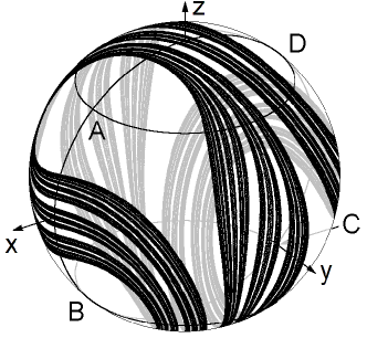
Figure 1: Attractor of the map (6) at $\varepsilon$=0.77 on the unit square

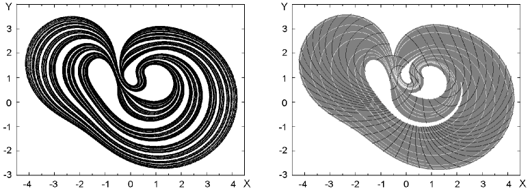
Figure 2: (a) Portrait of the attractor of the map (6) at $\varepsilon$=0.77 presented on a plane by means of the stereographic projection (7) and (b) disposition of stable (black) and unstable (white) manifolds in a domain $D$ (gray background) that contains the attractor

I argue that the attractor relates to the uniformly hyperbolic class, i.e. it is an attractor of Plykin type. To support this assertion let us turn to Fig. 2b illustrating location of stable and unstable manifolds in a domain D that contains the attractor. The stable and unstable manifolds are shown, respectively, by black an white curves, drawn on a gray background of the domain D. As seen, the unstable manifolds follow along filaments of the attractor, while the stable ones are transversal to the filaments. Mutual disposition of the stable and unstable manifolds certainly excludes possibility of tangencies, at least in the domain D.

An alternative approach to verification of the hyperbolicity can be based on the cone criterion known from the mathematical literature [1, 2, 3, 4, 5, 9]. Such calculations were performed on a base of methodology developed in Ref.[10], and the hyperbolicity was confirmed.

Lyapunov exponents were computed for the map ${\rm{\bf T}}$ by means of the procedure based on joint iterations of the map together with a collection of two sets of linearized equations for perturbation vectors. At each iteration step, these two vectors are orthogonalized, and normalized to a fixed constant. Lyapunov exponents are obtained as slopes of the straight lines approximating the accumulating sums of logarithms of the norm ratios for the vectors in dependence of the number of iterations [11]. In particular, at $\varepsilon$=0.77 the Lyapunov exponents are $\Lambda_{1}=0.9587$ and $\Lambda_{2}=-1.1406$. Then, the estimate of the attractor dimension from the Kaplan – Yorke formula yields $D_{KY}\approx 1+\Lambda_{1}/|\Lambda_{2}|=0.8405$.

One can accept an interpretation that an instant speed of a representative point on the sphere is determined by combination of two vector fields, which are switched on and off, turn by turn. One corresponds to dynamics during the stages of flow down, and another to the stages of differential rotation. Let us introduce angles $\bar{\alpha}$ and $\bar{\beta}$ determining directions of the fields, and coefficients $p$ and $q$ responsible for switching them on and off. We set $\bar{\alpha}=\bar{\beta}=\textstyle{\pi\over 4}(-1)^{[t/2]}-\textstyle{\pi\over 4},\,\,p=\textstyle{1\over 2}+\textstyle{1\over 2}(-1)^{[t]},\,\,\,\,q=\textstyle{1\over 2}(-1)^{[t/2]}-\textstyle{1\over 2}(-1)^{[t/2+1/2]}$. (Here [$\tau$] designates the integer part of $\tau$.) Setting $K=\pi/\sqrt{2}$, we write down the Eqs. (2)-(5) in a compact form:

$$\begin{array}[]{l}\dot{x}=-p\varepsilon y^{2}(x\cos\bar{\alpha}+z\sin\bar{\alpha})\cos\bar{\alpha}+qKy(-x\sin\bar{\beta}+z\cos\bar{\beta}+\textstyle{1\over{\sqrt{2}}})\cos\bar{\beta},\\ \dot{y}=p\varepsilon y(x\cos\bar{\alpha}+z\sin\bar{\alpha})^{2}-qK(x\cos\bar{\beta}+z\sin\bar{\beta})(-x\sin\bar{\beta}+z\cos\bar{\beta}+\textstyle{1\over{\sqrt{2}}}),\\ \dot{z}=-p\varepsilon y^{2}(x\cos\bar{\alpha}+z\sin\bar{\alpha})\sin\bar{\alpha}+qKy(-x\sin\bar{\beta}+z\cos\bar{\beta}+\textstyle{1\over{\sqrt{2}}})\sin\bar{\beta}.\\ \end{array}$$ (8)

As a next step, let us construct a version of the non-autonomous model containing only smooth functions. To do this, in Eqs. (8) we simply set

$$\alpha=\textstyle{\pi\over 4}\cos\textstyle{\pi\over 2}t,\,\,\beta=\textstyle{\pi\over 4}\sin\textstyle{\pi\over 2}t,\,\,p=1,\,\,\,q=\sin\textstyle{\pi\over 2}t.$$ (9)

Now, two vector fields, responsible for the flow down and for the differential rotation vary in time continuously and smoothly, undergoing rotations in space in such way that the original configuration is repeated with the period $T=4$. The second field oscillates, reversing the direction twice on a period. The time variations of one and other fields are shifted in phase relatively by a quarter of period. So, the extremal values of the fields are achieved turn by turn. The action of the fields at the extrema are mostly significant for motion of the representative points, hence, it is reasonable to specify the values at extrema, like in the original model. Because of structural stability of the hyperbolic attractor, one can hope that its nature remains the same after the modification, at least in a properly selected range of the parameters. As seen from computations, it is so, e.g. at $\varepsilon$=0.72 and $K$=1.9.

In contrast to the previous version of the model, the Poincaré map can not be expressed analytically. However, it may be easily realized by a computer program integrating the equations with a finite-difference method on a time period $T$ = 4.

We can exclude a redundant variable in the equations by means of the variable change (7), and rewrite them in terms of $W=X+iY$. After separation of the real and imaginary parts, we obtain

$$\begin{array}[]{c}\dot{X}=-2\varepsilon Y^{2}\Omega_{1}(X,Y,t)\left({\cos(\textstyle{\pi\over 4}\cos\textstyle{\pi\over 2}t)-X\sin(\textstyle{\pi\over 4}\cos\textstyle{\pi\over 2}t)}\right)\\ +KY\Omega_{2}(X,Y,t)\left({\cos(\textstyle{\pi\over 4}\sin\textstyle{\pi\over 2}t)-X\sin(\textstyle{\pi\over 4}\sin\textstyle{\pi\over 2}t)}\right)\,\sin\textstyle{{\pi t}\over 2},\\ \\ \dot{Y}=\varepsilon Y\Omega_{1}(X,Y,t)\left({2X\cos(\textstyle{\pi\over 4}\cos\textstyle{\pi\over 2}t)+(1-X^{2}+Y^{2})\sin(\textstyle{\pi\over 4}\cos\textstyle{\pi\over 2}t)}\right)\\ -K\Omega_{2}(X,Y,t)\left({X\cos(\textstyle{\pi\over 4}\sin\textstyle{\pi\over 2}t)+\textstyle{1\over 2}(1-X^{2}+Y^{2})\sin(\textstyle{\pi\over 4}\sin\textstyle{\pi\over 2}t)}\right)\,\sin\textstyle{{\pi t}\over 2},\\ \end{array}$$ (10)

where

$$\begin{array}[]{c}\Omega_{1}(X,Y,t)=\frac{2X\cos({\pi\over 4}\cos{\pi\over 2}t)+(1-X^{2}-Y^{2})\sin({\pi\over 4}\cos{\pi\over 2}t)}{(1+X^{2}+Y^{2})^{2}},\\ \\ \Omega_{2}(X,Y,t)=\frac{-2X\sin({\pi\over 4}\sin{\pi\over 2}t)+(1-X^{2}-Y^{2})\cos({\pi\over 4}\sin{\pi\over 2}t)}{(1+X^{2}+Y^{2})}+\frac{1}{\sqrt{2}}.\\ \end{array}$$ (11)

The expressions (10), (11) look a bit unwieldy, but this is, apparently, the first explicit example of a set of differential equations with smooth coefficients, which has attractor of Plykin type on a plane in the Poincaré cross-section.

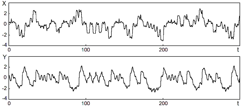
Figure 3: Variables $X$ and $Y$ versus time as obtained from numerical integration of the differential equations (10) at $\varepsilon$=0.72 and $K$=1.9. The plot relates to sustained chaotic regime associated with motion on the attractor; the transients are excluded

Figure 3 shows variables $X$ and $Y$ in dependence on time as obtained from numerical integration of the differential equations (10) at $\varepsilon$=0.72 and $K$=1.9, after exclusion of transients. Visually they look like realizations of random processes, as it should be for dynamics on the chaotic attractor.

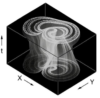
Figure 4: Portrait of attractor of the model (10) at $\varepsilon$=0.72 and $K$=1.9 in the extended three-dimensional phase space. The gray-scale technique is used: brighter tones correspond to relatively larger probability of visiting the pixels by orbits on the attractor

Figure 4 shows portrait of the attractor in the three-dimensional extended phase space ($X$, $Y$, $t)$. To make visible the inherent structure, the picture is presented in the gray-scale technique. Brighter tones correspond to relatively larger probability of visiting pixels by orbits on the attractor. Time interval on the vertical axis corresponds just to a period of variation of coefficients in the equations. In the cross-section of the attractor with the horizontal plane, one can observe an object with fractal structure, remarkably similar to that discussed in the context of the sphere map (see Fig. 2a). At a qualitative level, it may be regarded as an argument in favor of persistence of the hyperbolic attractor under modification of the model we undertake.

Computation of the Lyapunov exponents for the model (10) by means of the Benettin algorithm [11] at $\varepsilon$=0.72 and $K$=1.9 yields $\lambda_{1}\approx 0.221$ and $\lambda_{2}\approx-0.315$. It corresponds to the Lyapunov exponents of the Poincaré map $\Lambda_{1}=\lambda_{1}T\approx 0.884$ and $\Lambda_{2}=\lambda_{2}T\approx-1.260$. Estimate of the attractor dimension in the Poincaré section by the Kaplan – Yorke formula is $D_{KY}\approx 1.70$.

The hyperbolic nature of the attractor was verified by means of graphical representation of manifolds in the Poincaré section (like in Fig.2) and by the computations based on the cone criterion (in analogy with Ref. [11]). As follows from those results, attractor is hyperbolic in some parameter range around $\varepsilon$=0.72 and $K$=1.9. (More details will be published elsewhere.)

To conclude, this work puts into consideration a non-autonomous flow system manifesting chaotic dynamics associated with a hyperbolic strange attractor. In the stroboscopic Poincaré map it is attractor of Plykin type. In fact, I present two versions of the model. In the first version the evolution consists of successive stages, and the differential equations have piecewise continuous dependency of coefficients on time. The Poincaré map is expressed analytically, as a map on a sphere In the second version, the system is modified in such way that it is governed by a set of differential equations with smooth coefficients. The modification does not alter the hyperbolic nature of the chaotic attractor due to structural stability intrinsic to this object. As the system has the minimal phase space dimension required for existence of a hyperbolic strange attractor, its investigation, including verification of the hyperbolicity criteria is essentially simpler, in comparison with models suggested earlier as examples of attractors of Smale-Williams type [10, 12, 13]. Appearance of concrete examples of systems with hyperbolic strange attractors is of evident significance both from the point of view of complementation of mathematical concepts with concrete and visible context (see e.g. Ref. [14]), and for exploiting these concepts in applications. Hyperbolic chaotic systems may be of special interest for applications due to structural stability, that means insensitivity of the generated chaos to variations of parameters, characteristics of elements, technical fluctuations etc.

The work was performed, in part, during a visit of the author to the Group of Statistical Physics and Theory of Chaos in Potsdam University. The research is supported by RFBR-DFG grant 08-02-91963 and by grant 2.1.1/1738 of Ministry of Education and Science of Russian Federation in a frame of program of Development of Scientific Potential of Higher Education.

References

- [1] Eckmann J.-P. and Ruelle D. Ergodic theory of chaos and strange attractors. Rev. Mod. Phys. 1985;57:617-656.
- [2] Shilnikov L. Mathematical Problems of Nonlinear Dynamics: A Tutorial. International Journal of Bifurcation and Chaos. 1997;7:1353-2001.
- [3] Katok A. and Hasselblatt B. Introduction to the Modern Theory of Dynamical Systems. Cambridge: Cambridge University Press; 1995.
- [4] Afraimovich V. and Hsu S.-B. Lectures on chaotic dynamical systems. Somerville, MA: International Press; 2003.
- [5] Hasselblatt B. and Pesin Y. Hyperbolic dynamics. Scholarpedia, 2008;3(6):2208.
- [6] Plykin R.V. Sources and sinks of A-diffeomorphisms of surfaces. Math. USSR Sb. 1974; 23(2):233-253.
- [7] Hunt T.J. and MacKay R.S. Anosov parameter values for the triple linkage and a physical system with a uniformly chaotic attractor. Nonlinearity 2003;16:1499-1510.
- [8] Belykh V., Belykh I. and Mosekilde E. The hyperbolic Plykin attractor can exist in neuron models. International Journal of Bifurcation and Chaos 2005:15;3567-3578.
- [9] Hunt T.J. Low Dimensional Dynamics: Bifurcations of Cantori and Realisations of Uniform Hyperbolicity, PhD Thesis. Cambridge: Univercity of Cambridge; 2000.
- [10] Kuznetsov S.P. and Sataev I.R. Hyperbolic attractor in a system of coupled non-autonomous van der Pol oscillators: Numerical test for expanding and contracting cones. Physics Letters A 2007;365:97-104.
- [11] Benettin G., Galgani L., Giorgilli A., Strelcyn J.-M. Lyapunov characteristic exponents for smooth dynamical systems and for Hamiltonian systems: A method for computing all of them. Meccanica 1980;15: 9-30.
- [12] Kuznetsov S.P. Example of a Physical System with a Hyperbolic Attractor of the Smale-Williams Type. Phys. Rev. Lett. 2005:95;144101.
- [13] Kuznetsov S.P. and Pikovsky A. Autonomous coupled oscillators with hyperbolic strange attractors. Physica D 2007;232:87–102.
- [14] Coudene Y. Pictures of Hyperbolic Dynamical Systems. Notices of the American Mathematical Society 2006:53(1);8-13.