Infinitesimally Robust Estimation in General
Smoothly Parametrized Models

Abstract

We describe the shrinking neighborhood approach of Robust Statistics, which applies to general smoothly parametrized models, especially, exponential families. Equal generality is achieved by object oriented implementation of the optimally robust estimators. We evaluate the estimates on real datasets from literature by means of our R packages ROptEst and RobLox.

Keywords: Exponential family; Influence curves; Asymptotically linear estimators; Shrinking contamination and total variation neighborhoods; One-step construction; Minmax MSE

1 Introduction

Following Huber (1997), p 61, the purpose of robustness is “to safeguard against deviations from the assumptions, in particular against those that are near or below the limits of detectability”.
The infinitesimal approach of Huber–Carol (1970), Rieder (1978) and Rieder (1980), Bickel (1981), Rieder (1994) to robust testing and estimation, respectively, takes up this aim by employing shrinking neighborhoods of the parametric model, where the shrinking rate $n^{-1/2}$, as the sample size $n\to\infty$, may be deduced in a testing setup; confer Ruckdeschel (2006).
It is true that Huber’s own minimum Fisher information approach refers to (small) neighborhoods of fixed size; cf. Huber (1981). But it only treats variance, sets bias $=0$ by assuming symmetry, and is restricted to Tukey-type neighborhoods about location or scale models. It has not been extended to simultaneous location and scale, let alone to more general models. Fraiman et al. (2001) derive MSE optimality on fixed size neighborhoods. In situations beyond one-dimensional location, however, they do not determine a solution in closed form either. The infinitesimal approach, on the contrary, provides closed-form robust solutions for general models (cf. Section 2.1) and fairly general risks based on variance and bias (cf. Ruckdeschel and Rieder (2004)).

As noted by Huber (p 291 of Huber (1981)), in view of Theorem 3.7 of Rieder (1978), there is a close relation between the infinitesimal neighborhood approach and Hampel’s Lemma 5 (cf. Hampel (1968)); see also Theorem 3.2 of Rieder (1980) and Theorem 5.5.7 of Rieder (1994). Differences to Hampel et al. (1986) nevertheless exist and concern:

• definition of the influence curve,

• necessity of the form of the optimally robust influence curves,

• optimality criterion: MSE and even more general criterions,

• determination of the bias bound (sensitivity),

• uniform asymptotics on neighborhoods, and

• coverage of more models.

A fourth robustness approach pursues efficiency in the ideal model subject to a high breakdown point; confer for example Maronna et al. (2006), Sections 5.6.3, 5.6.4 and 6.4.5. A high breakdown, though, may easily be incorporated in our approach: Given some starting estimator $\hat{\theta}_{n}$, we construct our optimal estimators $S_{n}$ as one-step estimates,

$$S_{n}=\hat{\theta}_{n}+n^{-1}\bigl{(}\psi_{\hat{\theta}_{n}}(x_{1})+\cdots+\psi_{\hat{\theta}_{n}}(x_{n})\bigr{)}$$ (1)

cf. Section 4. The procedure is called one-step re-weighting in Section 5.6.3 of Maronna et al. (2006) and has already been used in the Princeton robustness study (cf. Andrews et al. (1972)). Thus, if $|\psi_{\theta}(x)|\leq b$, also $|S_{n}-\hat{\theta}_{n}|\leq b$. Consequently, the breakdown point of the starting estimator $\hat{\theta}_{n}$ is inherited to our estimator $S_{n}$. Given the high breakdown, however, we do not consider robustness as settled, then striving just for high efficiency in the ideal model. Our primary aim stays minmax MSE on shrinking neighborhoods about the ideal model, which altogether complies with Huber (1997), p 61, that “a high breakdown point is nice to have if it comes for free”.

The organisation of the paper is as follows: We review the theory of asymptotic robustness on shrinking neighborhoods, add some recent results and spezialize. Then, we compute and apply the infinitesimal robust estimators to datasets from literature using our R packages ROptEst (general models) and RobLox (normal location and scale); confer R Development Core Team (2008), Kohl and Ruckdeschel (2008c) and Kohl (2008). Appplications of infinitesimal neighborhood robustness to time series will be the subject of another paper.

2 Setup

2.1 General Smoothly Parametrized Models

Denoting by ${\cal M}_{1}({\cal A})$ the set of all probability measures on some measurable space $(\Omega,{\cal A})$, we consider a parametric model ${\cal P}=\{P_{\theta}\,|\,\theta\in\Theta\}\subset{\cal M}_{1}({\cal A})$, whose parameter space $\Theta$ is an open subset of some finite-dimensional $\mathbb{R}^{k}$, and which is dominated: $dP_{\theta}=p_{\theta}\,d\mu$ ($\theta\in\Theta$). At any fixed $\theta\in\Theta$, model ${\cal P}$ is required to be $L_{2}$ differentiable, that is, to have $L_{2}$ differentiable square root densities such that, in $L_{2}(\mu)$, as $t\to 0$,

$$\sqrt{p_{\theta+t}}\,=\sqrt{p_{\theta}}\,(1+\textstyle\frac{1}{2}t^{\prime}\Lambda_{\theta})+\mathop{\rm{{}o{}}}\nolimits(|t|)$$ (2)

The $\mathbb{R}^{k}$-valued function $\Lambda_{\theta}\in L_{2}^{k}(P_{\theta})$ is called $L_{2}$ derivative, and its covariance ${\cal I}_{\theta}=\mathop{\rm{{}E{}}}\nolimits_{\theta}\Lambda_{\theta}\Lambda_{\theta}^{\prime}$ under $P_{\theta}$ is the Fisher information of ${\cal P}$ at $\theta$, required of full rank $k$. This type of differentiability is implied by continuous differentiability of $p_{\theta}$ and continuity ${\cal I}_{\theta}$, with respect to $\theta$, and then $\Lambda_{\theta}=\frac{\partial}{\partial\theta}\log p_{\theta}$. Confer e.g. Lemma A.3 of Hajek (1972), Section 1.8 of Witting (1985), Section 2.3 of Rieder (1994), Rieder and Ruckdeschel (2001).
Our main applications in this article concern exponential families, in which case

$$p_{\theta}(x)=\exp\bigl{\{}\zeta(\theta)^{\prime}T(x)-\beta(\theta)\bigr{\}}h(x)$$ (3)

with some measurable functions $\zeta\colon\Theta\to\mathbb{R}^{k}$, $h\colon\Omega\to[\hskip 0.83313pt0,\infty)$, $T\colon\Omega\to\mathbb{R}^{k}$ of positive definite covariance $\mathop{\rm Cov}\nolimits_{\theta}T\succ 0$, and the normalizing constant $\beta(\theta)$. Then ${\cal P}$ forms a $k$-dimensional exponential family of full rank. The natural parameter space $Z_{*}$ consists of all $\zeta$-values such that $0<\int\exp\big{\{}\zeta^{\prime}T(x)\big{\}}h(x)\,\mu(dx)<\infty$. ${\cal P}$ is $L_{2}$ differentiable under the following assumptions: $\zeta$ continuously differentiable in $\theta\in\Theta$ with regular Jacobian matrix ${\cal J}_{\zeta}$, and $\zeta(\Theta)\subset Z_{*}^{\rm o}$ (interior). And then,

$$\Lambda_{\theta}(x)={\cal J}_{\zeta}^{\prime}\big{(}T(x)-\mathop{\rm{{}E{}}}\nolimits_{\theta}T\big{)}\qquad{\cal I}_{\theta}={\cal J}_{\zeta}^{\prime}\mathop{\rm Cov}\nolimits_{\theta}(T){\cal J}_{\zeta}$$ (4)

where $\mathop{\rm{{}E{}}}\nolimits_{\theta}$ denotes expectation under $P_{\theta}$. The result mentioned in van der Vaart (1998), Example 7.7, is proven in Kohl (2005), Lemma 2.3.6 (a). In what follows, the parametric model ${\cal P}$ is assumed $L_{2}$ differentiable at any $\theta\in\Theta$.

2.2 Asymptotically Linear Estimators

The founders of robust statistics have defined influence curves (IC) as Gâteaux derivatives of statistical functionals; confer Section 2.5 of Huber (1981) and Section 2.1 of Hampel et al. (1986). The classical definition, however, remains vague. Even if such a derivative exists, the definition is not strong enough to cover the empirical; confer Reeds (1976) and Fernholz (1983). Our approach is different: Since most proofs of asymptotic normality in the i.i.d. case amount to an estimator expansion with the IC as summands, we define the set of all (square integrable, $\mathbb{R}^{k}$-valued) ICs at $P_{\theta}$ beforehand by

$$\Psi(\theta)=\big{\{}\psi_{\theta}\in L_{2}^{k}(P_{\theta})\mid\mathop{\rm{{}E{}}}\nolimits_{\theta}\psi_{\theta}=0,\;\mathop{\rm{{}E{}}}\nolimits_{\theta}\psi_{\theta}\Lambda_{\theta}^{\prime}={\mathbb{I}}_{k}\big{\}}$$ (5)

where ${\mathbb{I}}_{k}$ denotes the $k\times k$ identity matrix. Then we define asymptotically linear (AL) estimators $S$ to be any sequence of estimators $S_{n}:\Omega^{n}\to\mathbb{R}^{k}$ such that for some $\psi_{\theta}\in\Psi(\theta)$, necessarily unique,

$$n^{1/2}(S_{n}-\theta)=n^{-1/2}\bigl{(}\psi_{\theta}(x_{1})+\cdots+\psi_{\theta}(x_{n})\bigr{)}+\mathop{\rm{{}o{}}}\nolimits_{P_{\theta}^{n}}(n^{0})$$ (6)

where $\mathop{\rm{{}o{}}}\nolimits_{P_{\theta}^{n}}(n^{0})\to 0$ in product $P_{\theta}^{n}$ probability as $n\to\infty$. Thus, the originally intended interpretation is achieved: $\psi_{\theta}(x_{i})$ represents the asymptotic, suitably standardized influence of observation $x_{i}$ on $S_{n}$. The class of AL estimators as introduced by Rieder (1980), Definition 1.1 and Remarks, and Rieder (1994), Section 4.2, covers M, L, R, S and MD (minimum distance) estimates.
By the Lindeberg-Lévy CLT, as $\psi_{\theta}\in L_{2}^{k}(P_{\theta})$, $\mathop{\rm{{}E{}}}\nolimits_{\theta}\psi_{\theta}=0$, AL estimators are asymptotically normal under $P_{\theta}^{n}$,

$$n^{1/2}(S_{n}-\theta)(P_{\theta}^{n})\mathrel{\mbox{$\longrightarrow$}\hbox to0.0pt{\hss\raisebox{-0.6458pt}{\makebox[7.5pt]{\scriptsize\rm w}}}}{\cal N}\,(0,\mathop{\rm Cov}\nolimits_{\theta}(\psi_{\theta}))$$ (7)

The third condition $\mathop{\rm{{}E{}}}\nolimits_{\theta}\psi_{\theta}\Lambda_{\theta}^{\prime}={\mathbb{I}}_{k}$ is equivalent to the locally uniform extension of (7), with $\theta$ on the LHS replaced by $\theta_{n}$ with $\limsup_{n\to\infty}\sqrt{n}\,|\theta_{n}-\theta|<\infty$.
For the asymptotic variance under $P_{\theta}$, the Cramér-Rao bound holds,

$$\mathop{\rm Cov}\nolimits_{\theta}(\psi_{\theta})\succeq{\cal I}_{\theta}^{-1}=\mathop{\rm Cov}\nolimits_{\theta}(\psi_{h,\theta})\,,\qquad\psi_{\theta}\in\Psi_{\theta}$$ (8)

with equality iff $\psi_{\theta}=\psi_{h,\theta}:={\cal I}_{\theta}^{-1}\Lambda_{\theta}$, the classical scores.

2.3 Infinitesimal Perturbations

The i.i.d. observations $x_{1},\dots,x_{n}$ may now follow any law $Q$ in some neighborhood about $P_{\theta}$. In this article , the type of neighborhoods in Rieder (1994) will be restricted to (convex) contamination ($*=c$) and total variation ($*=v$). Delegating the total variation case to Appendix A, the system ${\cal U}_{c}(\theta)$ thus consists of all contamination neighborhoods

$$U_{c}(\theta,s)=\big{\{}(1-s)P_{\theta}+s\,Q\,\big{|}\,Q\in{\cal M}_{1}({\cal A})\big{\}}\,,\qquad 0\leq s\leq 1$$ (9)

Subsequently, $s=s_{n}=rn^{-1/2}$ for starting radius $r\in[\hskip 0.83313pt0,\infty)$ and $n\to\infty$.

Remark 1.

Under $Q$, still the parameter $\theta$ has to be estimated. Since the equation $Q=P_{\theta}+(Q-P_{\theta})$ involving the nuisance component $Q-P_{\theta}$, may have multiple solutions $\theta$, the parameter $\theta$ is no longer identifiable. This problem has been dealt with by estimating functionals that extend the parametrization to the neighborhoods. As noted in Section 4.3.3 of Rieder (1994), however, both approaches lead to the same optimally robust ICs and procedures once the choice of the functional is subjected to robustness criteria.

We now fix $\theta\in\Theta$ and introduce the bounded tangents at $P_{\theta}$,

$$Z_{\infty}(\theta)=\big{\{}q\in L_{\infty}(P_{\theta})\,|\,\mathop{\rm{{}E{}}}\nolimits_{\theta}q=0\big{\}}$$ (10)

Along any $q\in Z_{\infty}(\theta)$ and for starting radius $r\in[0,\infty)$, simple perturbations are defined by

$$dQ_{n}(q,r)=\big{(}1+rn^{-1/2}q\,\big{)}dP_{\theta}$$ (11)

provided that $n^{1/2}\geq-r\inf_{P_{\theta}}q$, where $\inf_{P_{\theta}}$ denotes the $P_{\theta}$-essential infimum. AL estimators, under such simple perturbations, are still asymptotically normal,

$$n^{1/2}(S_{n}-\theta)\big{(}Q_{n}^{n}(q,r)\big{)}\mathrel{\mbox{$\longrightarrow$}\hbox to0.0pt{\hss\raisebox{-0.6458pt}{\makebox[7.5pt]{\scriptsize\rm w}}}}{\cal N}_{k}\big{(}r\mathop{\rm{{}E{}}}\nolimits_{\theta}\psi_{\theta}q,\,\mathop{\rm Cov}\nolimits_{\theta}(\psi_{\theta})\big{)}$$ (12)

with bias $r\mathop{\rm{{}E{}}}\nolimits_{\theta}\psi_{\theta}q$. We have $Q_{n}(q,r)\in U_{c}(\theta,rn^{-1/2})$ iff $q\in{\cal G}_{c}(\theta)$ for the class

$${\cal G}_{c}(\theta)=\big{\{}q\in Z_{\infty}(\theta)\mid\inf\nolimits_{P_{\theta}}q\geq-1\big{\}}$$ (13)

Confer Rieder (1994), proof to Proposition 4.3.6 and Lemma 5.3.1.

3 Optimally Robust Influence Curves

3.1 Maximum Risk

Our aim is minmax risk. Employing a continuous loss function $\ell\colon\mathbb{R}^{k}\to[\hskip 0.83313pt0,\infty)$, the asymptotic maximum risk of any estimator sequence on contamination neighborhoods about $P_{\theta}$ of size $rn^{-1/2}$ is

$$\lim_{M\to\infty}\lim_{n\to\infty}\sup\limits_{Q\in U_{c}(\theta,rn^{-1/2})}\int\ell_{M}\big{(}n^{1/2}(S_{n}-\theta)\big{)}\,dQ_{n}^{n}$$ (14)

where, for ease of attainability of the minimum risk, the truncated loss functions $\ell_{M}=\min\{M,\ell\}$ are employed. A further simplified and smaller risk is obtained by a restriction to simple perturbations $Q_{n}=Q_{n}(q,r)$ with $q\in{\cal G}_{c}(\theta)$ and the interchange of $\sup_{q\in{\cal G}_{c}(\theta)}$, $\lim_{M\to\infty}$, and $\lim_{n\to\infty}$.
The fixed $\theta$ will be dropped from notation henceforth whenever feasible. Thus, for an AL estimator $S=(S_{n})$ with IC $\psi$ at $P=P_{\theta}$, and $Z\sim{\cal N}_{k}\bigl{(}0,\mathop{\rm Cov}\nolimits(\psi)\bigr{)}$,

$$\sup_{q\in{\cal G}_{c}(\theta)}\lim_{M\to\infty}\lim_{n\to\infty}\int\ell_{M}\bigl{(}n^{1/2}(S_{n}-\theta)\bigr{)}\,dQ_{n}^{n}(q,r)=\sup_{q\in{\cal G}_{c}(\theta)}\mathop{\mbox{\hMtenrm E}}\nolimits\ell\bigl{(}r\mathop{\rm{{}E{}}}\nolimits\psi q+Z\bigr{)}$$ (15)

For the square $\ell(z)=|z|^{2}$, the (maximum, asymptotic) MSE is obtained as weighted sum of the $L_{2}$- and $L_{\infty}$-norms of $\psi$ under $P$,

$$\displaystyle\mathop{\rm MSE}\nolimits(\psi,r)=E|\psi|^{2}+r^{2}\omega_{c}^{2}(\psi)$$ (16)

$$\displaystyle\omega_{c}(\psi)=\sup\big{\{}|\mathop{\rm{{}E{}}}\nolimits\psi q|\,\big{|}\,q\in{\cal G}_{c}(\theta)\big{\}}=\sup\nolimits_{P}|\psi|$$

the $P$-essential sup of $|\psi|$; confer Sections 5.3.1 and 5.5.2 of Rieder (1994).
Other (convex, monotone) combinations of bias and variance (e.g., $L_{p}$-risks) have been considered in Ruckdeschel and Rieder (2004).
A suitable construction achieves that, in case of the optimally robust estimator, risk (14) is not larger than the simplified risk (15); confer Section 4 below.

3.2 Minmax Mean Square Error

The optimally robust $\psi^{\star}$, the unique solution to minimize $\mathop{\rm MSE}\nolimits(\psi,r)$ among all $\psi\in\Psi$, is given in Theorem 5.5.7 of Rieder (1994): There exist some vector $z\in\mathbb{R}^{k}$ and matrix $A\in\mathbb{R}^{k\times k}$, $A\succ 0$, such that

$$\displaystyle\psi^{\star}=A(\Lambda-z)w\,,\qquad w=\min\bigl{\{}1,\,b\,|A(\Lambda-z)|^{-1}\bigr{\}}$$ (18)

$$\displaystyle r^{2}b=\mathop{\rm{{}E{}}}\nolimits(|A(\Lambda-z)|-b)_{+}$$

$$\displaystyle 0=\mathop{\rm{{}E{}}}\nolimits(\Lambda-z)w\,,\qquad A^{-1}=\mathop{\rm{{}E{}}}\nolimits(\Lambda-z)(\Lambda-z)^{\prime}w$$

Conversely, form (18)–(20) suffices for $\psi^{\star}$ to be the solution.
The proof uses the Lagrange multipliers supplied by Rieder (1994), Appendix B.
The minmax solution to the more general risks considered in Ruckdeschel and Rieder (2004) also is a MSE solution with suitably transformed bias weight; confer their Theorem 4.1 and equation (4.7).
The matrix $A$, in case $r=0$, equals inverse Fisher information ${\cal I}^{-1}$, which appears in the Cramér-Rao bound (8). In general, $A$ is defined by (19) and (20) only implicitly. It is surprising that the statistical interpretation in terms of minimum risk obtains in the extension, with bias now involved.

Theorem 1.

For any $r\in(0,\infty)$ and $\psi\in\Psi$ we have

$$\mathop{\rm MSE}\nolimits(\psi,r)\geq\mathop{\rm tr}\nolimits A=\mathop{\rm MSE}\nolimits(\psi^{\star},r)$$ (21)

where equality holds in the first place iff $\psi=\psi^{\star}$ defined by (18)–(20).

3.3 Relative MSE

The starting radius $r$ for the neighborhoods $U_{c}(\theta,rn^{-1/2})$, on which the minmax MSE solution $\psi^{\star}=\psi^{\star}_{r}$ depends, will often be unknown or only known to belong to some interval $[r_{\rm lo},r_{\rm up})\subset[\hskip 0.83313pt0,\infty)$. In this situation that $\psi^{\star}_{s}$ is used when in fact $\psi^{\star}_{r}$ is optimal, we introduce the relative MSE of $\psi^{\star}_{s}$ at radius $r$,

$$\mathop{\rm relMSE}\nolimits(\psi^{\star}_{s},r)=\mathop{\rm MSE}\nolimits(\psi^{\star}_{s},r)\big{/}\mathop{\rm MSE}\nolimits(\psi^{\star}_{r},r)$$ (22)

For any radius $s\in[r_{\rm lo},r_{\rm up})$ the $\sup_{r}\mathop{\rm relMSE}\nolimits(\psi_{s}^{\star},r)$ is attained at the boundary,

$$\sup_{r\in[r_{\rm lo},r_{\rm up})}\mathop{\rm relMSE}\nolimits(\psi_{s}^{\star},r)=\mathop{\rm relMSE}\nolimits(\psi_{s}^{\star},r_{\rm lo})\lor\mathop{\rm relMSE}\nolimits(\psi_{s}^{\star},r_{\rm up})$$ (23)

A least favorable radius $r_{0}$ is defined by achieving $\inf_{s}$ of $\sup_{r}\mathop{\rm relMSE}\nolimits(\psi^{\star}_{s},r)$, that is,

$$\inf_{s\in[r_{\rm lo},r_{\rm up})}\sup_{r\in[r_{\rm lo},r_{\rm up})}\mathop{\rm relMSE}\nolimits(\psi_{s}^{\star},r)=\sup_{r\in[r_{\rm lo},r_{\rm up})}\mathop{\rm relMSE}\nolimits(\psi_{r_{0}}^{\star},r)$$ (24)

and is characterized by $\mathop{\rm relMSE}\nolimits(\psi_{r_{0}}^{\star},r_{\rm lo})=\mathop{\rm relMSE}\nolimits(\psi_{r_{0}}^{\star},r_{\rm up})$.
The IC $\psi^{\star}_{r_{0}}$, respectively the AL estimator with this IC, are called radius-minmax (rmx) and recommended.
Confer Kohl (2005), in particular Lemma 2.2.3, and Rieder et al. (2008).
The recommendation is in some sense independent of the loss function: In case of unspecified radius (i.e., $r_{\rm lo}=0$, $r_{{\rm up}}=\infty$), the rmx IC is the same for a variety of loss functions satisfying a weak homogeneity condition; confer Ruckdeschel and Rieder (2004), Theorem 6.1.

3.4 Cniper Contamination

The notion is suited to demonstrate how relatively small outliers suffice to destroy the superiority of the classical procedure. Employing, for this purpose, contaminations $R_{n}:=(1-rn^{-1/2})P+rn^{-1/2}\mathop{\bf\rm{{}I{}}}\nolimits_{\{a\}}$ by Dirac measures in $a\in\mathbb{R}$, the asymptotic MSE of the classically optimal estimator (i.e., with IC $\psi_{h}={\cal I}^{-1}\Lambda$) under $R_{n}$ is $\mathop{\rm MSE}\nolimits_{a}(\psi_{h},r):=\mathop{\rm tr}\nolimits{\cal I}^{-1}+r^{2}|\psi_{h}(a)|^{2}$. Relating this quantity to the minmax MSE $=\mathop{\rm tr}\nolimits A$ (Theorem 1), we are interested in the set ${\cal C}$ of values $a\in\mathbb{R}$ such that $\mathop{\rm MSE}\nolimits_{a}(\psi_{h},r)>\mathop{\rm MSE}\nolimits(\psi^{\star}_{r},r)$; that is,

$$r^{2}|\psi_{h}(a)|^{2}>\mathop{\rm tr}\nolimits A-\mathop{\rm tr}\nolimits{\cal I}^{-1}$$ (25)

In all models we have considered so far, rather small values $a$ suffice to fulfill (25). In a Janus type pun on the words “nice” and “pernicious”, the boundary values of ${\cal C}$ are called cniper points (acting like a sniper); confer Ruckdeschel (2004) and Kohl (2005), Introduction.

4 Estimator Construction

Given the optimally robust IC $\psi^{\star}_{\theta}$, one for each $\theta\in\Theta$, the problem is to construct an estimator $S^{\star}=(S_{n}^{\star})$ that is AL at each $\theta$ with IC $\psi^{\star}_{\theta}$. In addition, the construction should achieve that there is no increase from the simplified risk (15) to the asymptotic maximum MSE (14).
We require initial estimators $\sigma=(\sigma_{n})$ which are $n^{1/2}$ consistent on the full neighborhood system ${\cal U}_{c}(\theta)$; that is, for each $r\in[\hskip 0.83313pt0,\infty)$,

$$\lim_{M\to\infty}\limsup_{n\to\infty}\sup\big{\{}Q_{n}^{(n)}(n^{1/2}|\sigma_{n}-\theta|>M)\bigm{|}Q_{n,i}\in U_{c}(\theta,rn^{-1/2})\,\big{\}}=0$$ (26)

with $Q_{n}^{(n)}=Q_{n,1}\otimes\cdots\otimes Q_{n,n}$. For technical reasons, the $\sigma_{n}$ are in addition discretized in a suitable sense (cf. Rieder (1994), Section 6.4.2).
In this article, the optimally robust ICs $\psi_{\theta}^{\star}$ are bounded. Thus conditions (2)–(6) of Rieder (1994), p 247, on $(\psi_{\theta}^{\star})_{\theta\in\Theta}$ simplify drastically; namley, to continuity in sup-norm,

$$\lim_{\tau\to\theta}\sup\nolimits_{x\in\Omega}|\psi_{\tau}^{\star}(x)-\psi_{\theta}^{\star}(x)|=0$$ (27)

Then, according to Rieder (1994), Theorem 6.4.8 (b), the one-step estimator $S$,

$$S_{n}=\sigma_{n}+n^{-1}\bigl{(}\psi^{\star}_{\sigma_{n}}(x_{1})+\cdots+\psi^{\star}_{\sigma_{n}}(x_{n})\bigr{)}$$ (28)

where $\sigma_{n}=\sigma_{n}(x_{1},\ldots,x_{n})$, is uniformly asymptotically normal such that, for all arrays $Q_{n,i}\in U_{c}(\theta,rn^{-1/2})$ and each $r\in(0,\infty)$,

$$n^{1/2}(S_{n}-\theta-B_{n})(Q_{n}^{(n)})\mathrel{\mbox{$\longrightarrow$}\hbox to0.0pt{\hss\raisebox{-0.6458pt}{\makebox[7.5pt]{\scriptsize\rm w}}}}{\cal N}\,\bigl{(}0,\mathop{\rm Cov}\nolimits_{\theta}(\psi_{\theta}^{\star})\bigr{)}$$ (29)

with $B_{n}=n^{-1}\bigl{(}\int\psi_{\theta}^{\star}\,dQ_{n,1}+\cdots+\int\psi_{\theta}^{\star}\,dQ_{n,n}\bigr{)}$. Employing a version $\psi_{\theta}^{\star}$ of form (18)–(20) which is bounded pointwise by $b=b_{\theta}$, we obtain

$$|B_{n}|\leq\sup\nolimits_{x\in\Omega}|\psi_{\theta}^{\star}(x)|=b_{\theta}$$ (30)

Thus (29) ensures that risk (14) is not larger than the simplified risk (15).

Remark 2.

As initial estimators we prefer MD estimates, not primarily because of their breakdown point but because of their related tail behavior (cf. Ruckdeschel (2008a)) and their applicability in general models. In particular, both Kolmogorov and Cramér-von Mises MD (CvM) estimates may be employed (cf. Rieder (1994), Theorems 6.3.7 and 6.3.8), with an advantage of the latter—in view of the larger neighborhoods, to which its $n^{1/2}$ consistency extends, and the variance instability, for finite $n$, of the former (cf. Donoho and Liu (1988)). In particular models, other estimators may qualify as starting estimators and may even be preferable for computational reasons; e.g.; median, MAD in one-dim location and scale, minimum covariance determinant estimator in multivariate scale, least median of squares, and S estimates in linear regression; confer Rousseeuw and Leroy (1987) and Yohai (1987).

Remark 3.

Under additional smoothness, according to Ruckdeschel (2008a) and Ruckdeschel (2008b), assumption (26) of $n^{1/2}$ consistency may be weakened to only $n^{1/4+\delta}$ consistency, for some $\delta>0$. Consequently, for example, the least median of squares estimator may be employed as a high breakdown starting estimator. Ruckdeschel (2008b) gives other, partly more, partly less stringent conditions. Moreover, Ruckdeschel (2008a) ensures uniform integrability so as to dispense with the truncation of unbounded loss functions in (14).

The remainder of the section deals with condition (27). We assume that the Lagrange multipliers $A_{\theta}$ and $a_{\theta}:=A_{\theta}z_{\theta}$ in (18)–(20) are unique, and, as $\tau\to\theta$,

$$\displaystyle\Lambda_{\tau}(P_{\tau})\mathrel{\mbox{$\longrightarrow$}\hbox to0.0pt{\hss\raisebox{-0.6458pt}{\makebox[7.5pt]{\scriptsize\rm w}}}}\Lambda_{\theta}(P_{\theta})\,,\qquad\mathop{\rm tr}\nolimits{\cal I}_{\tau}\longrightarrow\mathop{\rm tr}\nolimits{\cal I}_{\theta}$$ (31)

$$\displaystyle\sup\limits_{x\in{\cal D}_{c}}|\Lambda_{\tau}(x)-\Lambda_{\theta}(x)|+\sup\limits_{x\in{}^{c}{\cal D}_{c}}\frac{|\Lambda_{\tau}(x)-\Lambda_{\theta}(x)|}{|A_{\theta}\Lambda_{\theta}(x)-a_{\theta}|}\longrightarrow 0$$ (32)

where ${\cal D}_{c}=\{\,x\in\Omega\mid|A_{t}\Lambda_{t}(x)-a_{t}|\leq b_{t}\;\mbox{for}\;t=\tau\>\mbox{or}\>t=\theta\,\}$. Then, by Kohl (2005), Theorem 2.3.3, condition (27) is fulfilled.

For example, in case of a location and scale with location parameter $\beta\in\mathbb{R}$ and scale parameter $\sigma\in(0,\infty)$, we have $\Lambda_{\theta}(x)=\sigma^{-1}\Lambda_{\theta_{0}}\bigl{(}(x-\beta)/\sigma\bigr{)}$, hence $\Lambda_{\theta}(P_{\theta})=\sigma^{-1}\Lambda_{\theta_{0}}(P_{\theta_{0}})$ and ${\cal I}_{\theta}=\sigma^{-2}{\cal I}_{\theta_{0}}$, where $\theta=(\beta,\sigma)^{\prime}$ and $\theta_{0}=(0,1)^{\prime}$. Therefore, (31) is fulfilled. Condition (32) needs further checking but seems plausible as $\Lambda_{\theta_{0}}$ is continuous (if the model is to be $L_{2}$ differentiable).

In the case of an $L_{2}$ differentiable exponential family, in view of (4), condition (31) is satisfied, while (32) holds according to Kohl (2005), Lemma 2.3.6.

5 Applications

5.1 Proposal

Based on the presented results we make the following proposal for applications:

Step 1: Decide on the ideal model.
Step 2: Decide on the type of neighborhood ($*=c$ or $*=v$).
Step 3: Determine lower and upper bounds $s_{\rm lo}$, $s_{\rm up}$ for the size $s=s_{n}$ of the neighborhoods $U_{*}(\theta,s)$ to be taken into account.
Step 4: Put $r_{\rm lo}=n^{1/2}s_{\rm lo}$, $r_{\rm up}=n^{1/2}s_{\rm up}$, and compute the rmx IC for $[\hskip 0.83313ptr_{\rm lo},r_{\rm up}]$.
Step 5: Evaluate an appropriate starting estimator.
Step 6: Determine the rmx estimator using the one-step construction.

Our R packages RobLox (cf. Kohl (2008)) and ROptEst (cf. Kohl and Ruckdeschel (2008c)) provide an easy way to perform steps 4–6 making use of our packages distr (cf. Ruckeschel et al. (2006)), distrEx (cf. Ruckeschel et al. (2006)), distrMod (cf. Ruckdeschel et al. (2008)), RandVar (cf. Kohl and Ruckdeschel (2008a)) and RobAStBase (cf. Kohl and Ruckdeschel (2008b)).
The implementation of these packages heavily relies on S4 classes and methods; confer Chamber (1998). Based on this object orientated approach package ROptEst provides an implemenation that (so far) works for all(!) $L_{2}$ differentiable parametric models which are based on a univariate distribution.
In the sequel, we will demonstrate the use of packages RobLox and ROptEst by application to some datasets from literature.

5.2 Normal Location and Scale

We consider the following $24$ measurements (in parts per million) of copper in wholemeal flour (cf. Analytical Methods Committee (1989))

          2.20  2.20  2.40  2.40  2.50  2.70  2.80  2.90
          3.03  3.03  3.10  3.37  3.40  3.40  3.40  3.50
          3.60  3.70  3.70  3.70  3.70  3.77  5.28 28.95

where the value $28.95$ is clearly conspicuous. In agreement with Maronna et al. (2006), Section 2.1, in view of the majority of the data, we assume normal location and scale as the ideal model, $P_{\theta}={\cal N}(\mu,\sigma^{2})$ with $\theta=(\mu,\sigma)^{\prime}$, $\mu\in\mathbb{R}$, $\sigma\in(0,\infty)$. Let us stick to contamination neighborhoods ($*=c$). We assume that roughly 1–5 observations, that is, roughly 5–20% of the $24$ observations are erroneous. Then the matrix $A$ and centering vector $a=Az$ in (18)–(20), by absolute continuity of the normal distribution, are unique. Since normal location and scale also is an $L_{2}$ differentiable exponential family, the assumptions for our estimator construction are fulfilled. We choose the Cramér-von Mises MD estimator (CvM) as initial estimator.
The following R code shows how function roptest of package ROptEst can be applied to perform the computations, where $x$ represents the data,

R > roptest(x = x, L2Fam = NormLocationScaleFamily(),
            neighbor = ContNeighborhood(), eps.lower = 0.05,
            eps.upper = 0.20, distance = CvMDist)

More specified to the normal ideal model is the function roblox of package RobLox, which only works for, and is optimized for speed in, normal location and scale. It uses median and MAD as starting estimates which is justified by Kohl (2005), Section 2.3.4.

R > roblox(x = x, eps.lower = 0.05, eps.upper = 0.20)

Table 1 shows the results of these computations as well as mean, standard deviation and some well-known robust estimators.

Table 1: Normal location and scale estimates

Estimator $\hat{\mu}$ $\hat{\sigma}$ mean & sd $4.28$ $5.30$ median & MAD $3.39$ $0.53$ Huber M (Proposal 2) $3.21$ $0.67$ Yohai MM $3.16$ $0.66$ CvM $3.23$ $0.67$ rmx (roptest) $3.16$ $0.66$ rmx (roblox) $3.23$ $0.64$

The robust estimators median & MAD – rmx (roblox) yield very similar results, while, obviously, mean and standard deviation represent the data badly. Figure 1 shows the location and scale parts of the rmx IC computed via function roblox. The location part of the rmx IC, as of any optimally robust IC, is redescending.

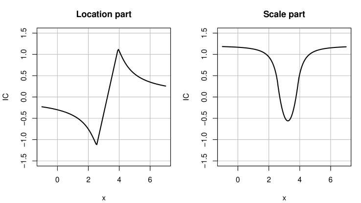
Figure 1: rmx IC computed via roblox.

Thus, redescending in our setup follows on optimality grounds. For another derivation of redescending $M$-estimators see Shevlyakov et al. (2008).
Based on these robust estimates, let us assume a mean of $\mu=3.2$ and a standard deviation of $\sigma=0.7$ for the ideal distribution $P_{\theta}={\cal N}(3.2,0.7^{2})$. For a contamination of $s_{n}=10\%$ at a sample size of $n=24$ (i.e., $r\approx 0.49$), the cniper points are calculated to $1.86$ and $4.54$, and ${\cal C}=(-\infty,1.86]\cup[4.54,\infty)$. Under any element of $U_{c}(\theta,s_{n})$ the probability of ${\cal C}$ is 5–15%, where $P_{\theta}({\cal C})=5.56\%$.

5.3 Gamma Model

We analyze the length of stays of 201 patients in the University Hospital of Lausanne during the year 2000 (cf. Hubert and Vandervieren (2006)). Following Marrazi et al. (1998), we use the Gamma model $p_{\theta}(x)=\Gamma(\alpha)^{-1}\sigma^{-\alpha}x^{\alpha-1}\,e^{-x/\sigma}$ with shape and scale parameters $\sigma,\alpha\in(0,\infty)$ and $\theta=(\sigma,\alpha)^{\prime}$. By Kohl (2005), Section 6.1, this exponential family is $L_{2}$ differentiable. We assume contamination neighborhoods ($*=c$) but, on visual inspection of the data, of only small size $0.5\%\leq s_{n}\leq 5\%$. Then, due to absolute continuity of $P=P_{\theta}$, equations (18)–(20) yield unique solutions $A$ and $a=Az$. Thus, the one-step construction of the rmx estimator, based on the CvM estimate, applies. The algorithm can be performed by applying function roptest of package ROptEst, where $x$ contains the data,

R > roptest(x = x, L2Fam = GammaFamily(),
            neighbor = ContNeighborhood(), eps.lower = 0.005,
            eps.upper = 0.05, distance = CvMDist)

a call, which is very similar to the one in the previous example. In fact, the unified call for roptest applies to any smooth model. Figure 2 compares the densities of the estimated Gamma distributions with the histogram of the data. Table 2 shows the results as well as the MLE and the CvM. Again, the MLE is strongly affected by a few very large observations whereas the robust estimators stay closer to the bulk of the data.

Figure 2: Observed frequencies and fitted Gamma densities.

Figure 3 shows scale and shape parts of the rmx IC (similarly, of any optimally robust IC; confer Kohl (2005), Figure 6.1).
Assuming the ideal Gamma distribution $P_{\theta}$ with $\theta=(5.0,1.9)^{\prime}$ and a contamination size $s_{n}=2.5\%$ at $n=201$ (i.e., $r\approx 0.35$), the cniper points are $0.62$ and $29.31$, and ${\cal C}=(-\infty,0.62]\cup[29.31,\infty)$. Under any element of $U_{c}(\theta,s_{n})$ the probability of ${\cal C}$ is 2.5–5%, where $P_{\theta}({\cal C})=2.63\%$.

Table 2: Gamma scale and shape estimates

Estimator MLE CvM rmx $\hat{\sigma}$ $7.00$ $6.53$ $4.97$ $\hat{\alpha}$ $1.61$ $1.54$ $1.86$

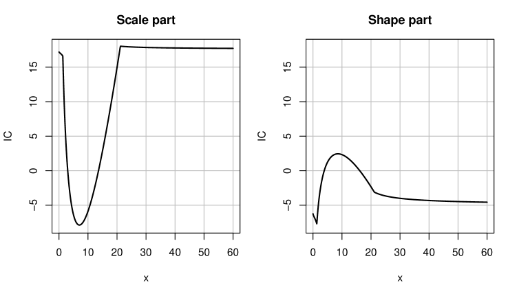
Figure 3: rmx IC computed via roptest.

5.4 Poisson Model

For the decay counts of polonium recorded by Rutherford and Geiger (1910),

     counts  0   1   2   3   4   5   6   7  8  9 10 11 12 13 14
  frequency 57 203 383 525 532 408 273 139 45 27 10  4  0  1  1

we assume the Poisson model $p_{\theta}(x)=e^{-\theta}\,\theta^{x}\!/x!$, which exponential family is $L_{2}$ differentiable in the paramter $\theta\in(0,\infty)$ (cf. Kohl (2005), Section 4.1).
For both contamination ($*=c$) and total variation neighborhoods ($*=v$) of size $0.01\leq s_{n}\leq 0.05$ we compute the rmx estimator. But, in case $*=c$, $a=Az$ may be non-unique, which happens if $\mathop{\rm med}\nolimits_{P}(\Lambda)$, the median of $\Lambda=\Lambda_{\theta}$ under $P=P_{\theta}$, is non-unique and $r=n^{1/2}s_{n}$ is $\geq$ the so called lower case radius $\bar{r}$ (cf. Kohl (2005), Section 2.1.2). The non-uniqueness of the median occurs for only countably many values $\theta$. Since, as our numerical evaluations show, already small deviations ($\sim\pm 10^{-8}$) from the exceptional values lead to a unique $a$, non-uniqueness may be neglected in practice; confer Kohl (2005), Sections 4.2.1 and 4.4. In case $*=v$, the one-step construction applies without restrictions; confer Appendix A. Then, using the CvM as starting estimator, the rmx estimators are obtained via the following calls to function roptest of package ROptEst, where $x$ contains the data,

R > roptest(x = x, L2Fam = PoisFamily(),
            neighbor = *, eps.lower = 0.01,
            eps.upper = 0.05, distance = CvMDist)

where * stands for ContNeighborhood() or TotalVarNeighborhood(), respectively. The results as well as MLE and CvM estimate are given in Table 3.

Table 3: Poisson mean estimates

Estimator MLE CvM rmx ($*=c$) rmx ($*=v$) $\hat{\theta}$ $3.8715$ $3.8953$ $3.9131$ $3.9133$

The estimates differ only slightly, as the data, in view of the observed and fitted frequencies in Figure 4, appears in very good agreement with the Poisson model.

Figure 4: Observed and fitted frequencies.

Figure 5 shows the rmx ICs for contamination and total variation neighborhoods. In fact, any optimally robust IC is of similar form (cf. Kohl (2005), Figures 4.1 ($*=c$) and 4.14 ($*=v$)).

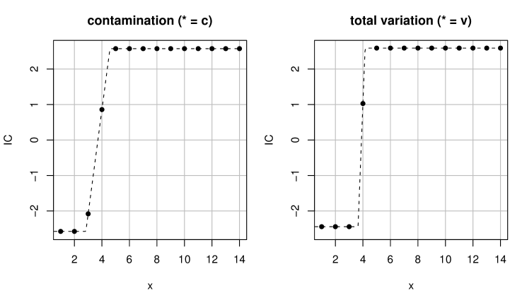
Figure 5: rmx IC computed via roptest for $*=c,v$.

Remark 4.

ICs are defined with respect to the ideal model, thus, in case of the Poisson model, on $\mathbb{N}_{0}$. If we want to allow distributions in the neighborhoods whose supports are more generally in $[\hskip 0.83313pt0,\infty)$, we only need to extend $\psi^{\star}$ from $\mathbb{N}_{0}$ to $[\hskip 0.83313pt0,\infty)$ such that $|\psi^{\star}(x)|\leq b$ for each $x>0$; confer (30) in the estimator construction.

Assuming the ideal Poisson distribution $P_{\theta}$ with $\theta=3.9$, neighborhood type $*=c$ and a contamination size $s_{n}=3\%$ at $n=2608$ (i.e., $r\approx 1.53$), we get the cniper points $1.26$ and $6.54$, and ${\cal C}=[0,1.26]\cup[6.54,\infty)$. Under any element of $U_{c}(\theta,s_{n})$ the probability of ${\cal C}$ is 19.5–22.5%, where $P_{\theta}({\cal C})=20.0\%$.

Appendix A Total variation neighborhoods ($*=v$)

The system ${\cal U}_{v}(\theta)$ consist of the closed balls of radius $s$ about $P_{\theta}$, in the total variation metric $d_{v}(Q,P_{\theta})=\sup_{A\in{\cal A}}|Q(A)-P_{\theta}(A)|$,

$$U_{v}(\theta,s)=\bigl{\{}Q\in{\cal M}_{1}({\cal A})\bigm{|}d_{v}(Q,P_{\theta})\leq s\bigr{\}}\,,\qquad 0\leq s\leq 1$$ (33)

which have the following representation in terms of contamination neighborhoods,

$$U_{v}(\theta,s)-P_{\theta}=\bigl{(}U_{c}(\theta,s)-P_{\theta}\bigr{)}-\bigl{(}U_{c}(\theta,s)-P_{\theta}\bigr{)}$$ (34)

In particular, $U_{c}(\theta,s)\subset U_{v}(\theta,s)$ follows. In our asymptotics, $s=s_{n}=rn^{-1/2}$ for some $r\in[\hskip 0.83313pt0,\infty)$, as the sample size $n\to\infty$. Corresponding simple perturbations $Q_{n}(q,r)$ are defined by (10) and (11) with tangents $q$ in the class

$${\cal G}_{v}(\theta)=\big{\{}q\in Z_{\infty}(\theta)\,\big{|}\,\mathop{\rm{{}E{}}}\nolimits_{\theta}|q|\leq 2\big{\}}={\cal G}_{c}(\theta)-{\cal G}_{c}(\theta)$$ (35)

We fix $\theta$ and drop it from notation. Then, with $\sup_{e}$ extending over all unit vectors $e$ in $\mathbb{R}^{k}$, the standardized (infinitesimal) bias term of an IC $\psi\in\Psi$ is

$$\omega_{v}(\psi)=\sup\bigl{\{}|\mathop{\rm{{}E{}}}\nolimits{\psi q}|\bigm{|}q\in{\cal G}_{v}(\theta)\bigr{\}}=\sup\nolimits_{e}\bigl{(}\sup\nolimits_{P}e^{\prime}\psi-\inf\nolimits_{P}e^{\prime}\psi\,\bigr{)}$$ (36)

The exact bias term in case $k>1$ is difficult to handle and has been dealt with only in exceptional cases (cf. Rieder (1994), p 205 and Theorem 7.4.17). The obvious bound $\omega_{c}(\psi)\leq\omega_{v}(\psi)\leq 2\,\omega_{c}(\psi)$ suggests an approximate solution by a reduction to the contamination case $*=c$ and radius $2\hskip 0.83313ptr$. An exact solution of the MSE problem with bias term $\omega_{v}$ is still possible in dimension $k=1$, in which case $\omega_{v}(\psi)=\sup_{P}\psi-\inf_{P}\psi$. In case $k=1$, the optimally robust IC $\psi^{\star}$, the unique solution to minimize $\mathop{\rm MSE}\nolimits(\psi,r)=\mathop{\rm{{}E{}}}\nolimits\psi^{2}+r^{2}\omega_{v}^{2}(\psi)$ among all ICs $\psi\in\Psi$ is provided by Rieder (1994), Theorem 5.5.7: For some numbers $c$, $b$, $A$,

$$\displaystyle\psi^{\star}=c\lor A\Lambda\land(c+b)$$ (37)

$$\displaystyle r^{2}b=\mathop{\rm{{}E{}}}\nolimits\big{(}c-A\Lambda)_{+}=\mathop{\mbox{\hMtenrm E}}\nolimits\big{(}A\Lambda-(c+b)\big{)}_{+}$$

$$\displaystyle\mathop{\mbox{\hMtenrm E}}\nolimits\bigl{(}c\vee A\Lambda\wedge(c+b)\bigr{)}\Lambda=1$$

Conversely, form (37)–(39) suffices for $\psi^{\star}$ to be the solution.

The solutions $A$, $b$ and $c$ of equations (37)–(39) are always unique, as discussed in Section B.1 below. Moreover, the condition that, as $\tau\to\theta$,

$$\sup_{x\in{\cal D}_{v}}|\Lambda_{\tau}(x)-\Lambda_{\theta}(x)|+\sup_{x\in{}^{c}{\cal D}_{v}}\frac{|\Lambda_{\tau}(x)-\Lambda_{\theta}(x)|}{|\Lambda_{\theta}(x)|}\longrightarrow 0$$ (40)

where ${\cal D}_{v}=\{\hskip 0.83313ptx\in\Omega\mid c_{t}\leq A_{t}\Lambda_{t}(x)\leq b_{t}+c_{t}\;\mbox{for}\;t=\tau\>\mbox{or}\>t=\theta\,\}$, has been verified by Kohl (2005), Lemma 2.3.6, in the case $*=v$, $k=1$, for $L_{2}$ differentiable exponential families. Thus, the one-step construction is valid.

Appendix B Auxiliary Results And One Proof

B.1 Boundedness, Uniqueness, Continuity Of Lagrange Multipliers

We discuss boundedness, uniqueness, and continuity of the Lagrange multipliers $A$, $a=Az$, $b$ and $c$ in the optimally robust IC $\psi^{\star}$. These properties are, on one hand, reassuring for the convergence of our numerical algorithms. On the other hand, they imply the continuity in sup-norm (27) required for the construction.

Boundedness Given $r>0$, bounds for the solutions $A$, $a=Az$, $b$ and $c$ of (18)–(20) and (37)–(39), respectively, are derived in Kohl (2005), Section 2.1.3. For example, $|a|\leq r^{2}b$ holds.

Uniqueness The Lagrange multipliers (like the separating hyperplanes) need not be unique; confer Rieder (1994), Remark B.2.10 (a). But, at least, $\mathop{\rm tr}\nolimits A$, $b$, and $c$ in (18)–(20) and (37)–(39), respectively, are unique since, in terms of the unique $\psi^{\star}$,

$$\mathop{\rm tr}\nolimits A=\mathop{\rm MSE}\nolimits(\psi^{\star},r)\,,\quad b=\omega_{*}(\psi^{\star})\,,\quad c=\inf\nolimits_{P}\psi^{\star}$$ (41)

If $k=1$ and $\mathop{\rm med}\nolimits_{P}(\Lambda)$ is unique, then $a$ is unique; Rieder (1994), Lemma C.2.4. In case $k=1$ and $\mathop{\rm med}\nolimits_{P}(\Lambda)$ is non-unique, then $a$ is unique for $r<\bar{r}$ (the so called lower case radius); confer Kohl (2005), Proposition 2.1.3.
In case $*=c$, $k\geq 1$, uniqueness of $A$ and $a$ is ensured by the assumption that

$$\mathop{\rm support}\Lambda(P)=\mathbb{R}^{k}$$ (42)

confer Rieder (1994), Remark 5.5.8. $A$ and $a$ are unique also under the more implicit condition that, for any hyperplane $H\subset\mathbb{R}^{k}$,

$$P(\Lambda\in H)<P(|\psi^{\star}|<b)$$ (43)

which certainly is satisfied if $P(\Lambda\in H)=0$ for any hyperplane $H$; that is,

$$e\in\mathbb{R}^{k}\,,\;\alpha\in\mathbb{R}\,,\;P(e^{\prime}\Lambda=\alpha)>0\;\Longrightarrow\;e=0$$ (44)

confer Rieder (1994), Section 5.5.3. Both (42) and (44) imply that ${\cal I}\succ 0$.

Continuity in $\theta$: Denote by $\psi_{\theta}^{\star}$ the MSE solution to variable parameter $\theta\in\Theta$ and fixed radius $r\in(0,\infty)$. Then, under assumption (31), we obtain

$$\mathop{\rm tr}\nolimits A_{\tau}\longrightarrow\mathop{\rm tr}\nolimits A_{\theta}\,,\quad b_{\tau}\longrightarrow b_{\theta}\,,\quad c_{\tau}\longrightarrow c_{\theta}$$ (45)

as $\tau\to\theta$. Provided that $A_{\theta}$ and $a_{\theta}$ are unique, moreover

$$A_{\tau}\longrightarrow A_{\theta}\,,\qquad a_{\tau}\longrightarrow a_{\theta}$$ (46)

Confer Kohl (2005), Theorem 2.1.11.

Continuity in $r$: Continuity in $r$ is needed for the rmx estimator. Denoting by $A_{r}$, $a_{r}=A_{r}z_{r}$, $b_{r}$, and $c_{r}$ the solutions of (18)–(20) and (37)–(39), respectively, for fixed $\theta$ and variable $r\in(0,\infty)$, Kohl (2005), Proposition 2.1.9, says that

$$\mathop{\rm tr}\nolimits A_{s}\longrightarrow\mathop{\rm tr}\nolimits A_{r}\,,\quad b_{s}\longrightarrow b_{r}\,,\quad c_{s}\longrightarrow c_{r}$$ (47)

as $s\to r$. Moreover, in case that $A_{r}$ and $a_{r}$ are unique,

$$A_{s}\longrightarrow A_{r}\,,\qquad a_{s}\longrightarrow a_{r}$$ (48)

For the rmx estimator, in addition some monotonicity in $r$ is needed and supplied by Ruckdeschel and Rieder (2004), Kohl (2005), and Rieder et al. (2008).

B.2 Proof of Theorem 1

$\mbox{minmaxMSE}=\mathop{\rm{{}E{}}}\nolimits|\eta|^{2}+r^{2}b^{2}=-\mathop{\rm{{}E{}}}\nolimits\eta^{\prime}(Y-\eta)+\mathop{\rm{{}E{}}}\nolimits\eta^{\prime}Y+r^{2}b^{2}$ with the abbreviations $\eta:=\psi^{\star}$, $Y:=A\Lambda$, where $\mathop{\rm{{}E{}}}\nolimits\eta^{\prime}Y=\mathop{\rm tr}\nolimits\mathop{\rm{{}E{}}}\nolimits\eta Y^{\prime}=\mathop{\rm tr}\nolimits A^{\prime}=\mathop{\rm tr}\nolimits A$ since $\mathop{\rm{{}E{}}}\nolimits\eta\Lambda^{\prime}={\mathbb{I}}_{k}$.

$*=c$: In this case, $\eta\neq Y$ iff $|Y|>b$, and thus $\mathop{\rm{{}E{}}}\nolimits\eta^{\prime}(Y-\eta)=b\mathop{\rm{{}E{}}}\nolimits(|Y|-b)_{+}=r^{2}b$.

$*=v$, $k=1$: In this case, $\mathop{\rm{{}E{}}}\nolimits\eta(Y-\eta)=b\mathop{\rm{{}E{}}}\nolimits(c-Y)_{+}=r^{2}b^{2}$.

References

- Analytical Methods Committee (1989) Analytical Methods Committee (1989). Robust statistics – how not to reject outliers. The Analyst, 114, 1693–1702.
- Andrews et al. (1972) Andrews D. F., Bickel P. J., Hampel F. R., Huber P. J., Rogers W. H., and Tukey J. W. (1972). Robust estimates of location. Survey and advances. Princeton University Press, Princeton, N. J..
- Bickel (1981) Bickel, P. J. (1981). Quelques aspects de la statistique robuste. Ecole d’ete de probabilites de Saint-Flour IX-1979, Lect. Notes Math. 876, 2–72.
- Chamber (1998) Chambers, J. M. (1998). Programming with data: a guide to the S language. Springer, New York.
- Donoho and Liu (1988) Donoho D. L. and Liu, R. C. (1988). Pathologies of Some Minimum Distance Estimators. Annals of Statistics 16(2),587–608.
- Feller (1968) Feller, M. (1968). An introduction to probability theory and its applications. I. Wiley, New York.
- Fernholz (1983) Fernholz, L.T. (1983). Von Mises Calculus for Statistical Functionals. Lecture Notes in Statistics #19. Springer-Verlag, New York.
- Fraiman et al. (2001) Fraiman, R., Yohai, V. J. and Zamar, R. H. (2001). Optimal robust -estimates of location. Ann. Stat., 29(1), 194–223.
- Hajek (1972) Hajek, J. (1972). Local asymptotic minimax and admissibility in estimation. Proc. 6th Berkeley Sympos. math. Statist. Probab., Univ. Calif. 1970, 1, 175–194.
- Hampel (1968) Hampel, F. R. (1968). Contributions to the theory of robust estimation. Dissertation, University of California, Berkely, CA.
- Hampel et al. (1986) Hampel, F. R., Ronchetti, E. M., Rousseeuw, P. J. and Stahel, W. A. (1986). Robust statistics. The approach based on influence functions. Wiley, New York.
- Huber (1964) Huber, P. J. (1964). Robust estimation of a location parameter. Ann. Math. Stat., 35, 73–101.
- Huber (1981) Huber, P. J. (1981). Robust statistics. Wiley, New York.
- Huber (1997) Huber, P. J. (1997). Robust statistical procedures. 2nd ed. CBMS-NSF Regional Conference Series in Applied Mathematics. 68. Philadelphia, PA: SIAM.
- Huber–Carol (1970) Huber–Carol, C. (1970). Étude asymptotique de tests robustes. Thèse de Doctorat, ETH Zürich.
- Hubert and Vandervieren (2006) Hubert, M. and Vandervieren, E. (2006). An Adjusted Boxplot for Skewed Distributions. Technical Report TR-06-11, KU Leuven, Section of Statistics, Leuven. URL http://wis.kuleuven.be/stat/robust/Papers/TR0611.pdf.
- Kohl (2005) Kohl, M. (2005). Numerical contributions to the asymptotic theory of robustness. Dissertation, University of Bayreuth, Bayreuth.
- Kohl (2008) Kohl, M. (2008). RobLox: Optimally robust influence curves for location and scale. R package version 0.6.1. URL http://robast.r-forge.r-project.org.
- Kohl and Ruckdeschel (2008a) Kohl, M., and Ruckdeschel, P. (2008a). RandVar: Implementation of random variables. R package version 0.6.6. URL http://robast.r-forge.r-project.org/
- Kohl and Ruckdeschel (2008b) Kohl, M. and Ruckdeschel, P. (2008b). RobAStBase: Robust Asymptotic Statistics. R package version 0.1.5. URL http://robast.r-forge.r-project.org.
- Kohl and Ruckdeschel (2008c) Kohl, M. and Ruckdeschel, P. (2008c). ROptEst: Optimally robust estimation. R package version 0.6.3. URL http://robast.r-forge.r-project.org.
- Marrazi et al. (1998) Marazzi, A., Paccaud, F., Ruffieux, C. and Beguin, C. (1998). Fitting the distributions of length of stay by parametric models. Medical Care, 36, 915–927.
- Maronna et al. (2006) Maronna, R. A., Martin, R. D. and Yohai, V. J. (2006). Robust Statistics: Theory and Methods. Wiley, New York.
- R Development Core Team (2008) R Development Core Team (2008). R: A language and environment for statistical computing. R Foundation for Statistical Computing, Vienna, Austria. ISBN 3-900051-07-0, URL http://www.R-project.org.
- Reeds (1976) Reeds, J.A. (1976). On the Definition of von Mises Functionals. Ph.D. Thesis, Harvard University, Cambridge.
- Rieder (1978) Rieder, H. (1978). A robust asymptotic testing model. Ann. Stat., 6, 1080–1094.
- Rieder (1980) Rieder, H. (1980). Estimates derived from robust tests. Ann. Stat., 8, 106–115.
- Rieder (1994) Rieder, H. (1994). Robust asymptotic statistics. Springer, New York.
- Rieder et al. (2008) Rieder, H., Kohl, M. and Ruckdeschel, P. (2008). The cost of not knowing the radius. Stat. Meth. & Appl., 17, 13–40.
- Rieder and Ruckdeschel (2001) Rieder, H. and Ruckdeschel, P. (2001). Short Proofs on –Differentiability. Stat. Decis., 19, 419–425.
- Rousseeuw and Leroy (1987) Rousseeuw, P.J. and Leroy, A.M. (1987). Robust Regression and Outlier Detection. Wiley, New York.
- Ruckdeschel (2006) Ruckdeschel, P. (2006). A Motivation for -Shrinking-Neighborhoods. Metrika, 63(3), 295–307
- Ruckdeschel (2004) Ruckdeschel, P. (2004). Higher Order Asymptotics for the MSE of M-Estimators on Shrinking Neighborhoods. Unpublished manuscript.
- Ruckdeschel (2008a) Ruckdeschel, P. (2008a). Uniform Integrability on Neighborhoods. In preparation.
- Ruckdeschel (2008b) Ruckdeschel, P. (2008b). Uniform Higher Order Asymptotics for Risks on Neighborhoods. In preparation.
- Ruckeschel et al. (2006) Ruckdeschel, P. and Kohl, M. and Stabla, T. and Camphausen, F. (2006). S4 classes for distributions. R News, 6(2), 2–6.
- Ruckdeschel et al. (2008) Ruckdeschel, P., Kohl, M., Stabla, T. and Camphausen, F. (2008). S4 Classes for Distributions—a manual for packages distr, distrSim, distrTEst, distrEx, distrMod, and distrTeach. Technical Report, Fraunhofer ITWM, Kaiserslautern, Germany.
- Ruckdeschel and Rieder (2004) Ruckdeschel, P. and Rieder, H. (2004). Optimal influence curves for general loss functions. Stat. Decis., 22, 201–223.
- Rutherford and Geiger (1910) Rutherford, E. and Geiger, H. (1910). The Probability Variations in the Distribution of alpha Particles. Philosophical Magazine, 20, 698–704.
- Shevlyakov et al. (2008) Shevlyakov, G., Morgenthaler, S. and Shurygin, A. (2008). Redescending M-estimators. J. Stat. Plan. Inference, 138(10), 2906–2917.
- van der Vaart (1998) van der Vaart, A. W. (1998). Asymptotic statistics. Cambridge Univ. Press., Cambridge.
- Witting (1985) Witting, H. (1985). Mathematische Statistik I: Parametrische Verfahren bei festem Stichprobenumfang. B.G. Teubner, Stuttgart.
- Yohai (1987) Yohai, V. J. (1987). High breakdown-point and high efficiency robust estimates for regression. Ann. Statist., 15(2), 642–656.