Pion masses in quasiconformal gauge field theories

Abstract

We study modifications to Weinberg-like sum rules in quasiconformal gauge field theories. Beyond the two Weinberg sum rules and the oblique $S$ parameter we study the pion mass and the $X$ parameter. Especially, we evaluate the pion mass for walking technicolour theories, in particular also minimal walking technicolour, and find contributions of the order of up to several hundred GeV.

Introduction. The Large Hadron Collider (LHC) has been built to help clarifying the mechanism for the breaking of the electroweak symmetry. Beyond the standard model, where the symmetry is broken by an elementary scalar Higgs particle, technicolour (TC) TC provides a possible mechanism which overcomes some of the deficiencies of the former. In TC the electroweak symmetry is broken by chiral symmetry breaking among additional fermions charged under the electroweak and the TC gauge groups. Three of the possibly more numerous Nambu–Goldstone modes are absorbed as longitudinal degrees of freedom of the electroweak gauge bosons. Walking WTC , that is, quasiconformal TC theories with techniquarks in higher dimensional representations are compatible with currently available precision data Dietrich:2005jn ; Dietrich:2006cm . Like everywhere in strongly interacting gauge theories effective Lagrangians are heavily used EFFECT ; Foadi:2007ue . In many cases the predictive power of these approaches is enhanced by enforcing the Weinberg sum rules EFFECT ; Foadi:2007ue ; Weinberg:1967kj .

Asymptotically free gauge field theories obey the Weinberg sum rules Weinberg:1967kj . It has been shown, however, that the second sum rule is modified Appelquist:1998xf in quasiconformal theories while the expression for the first remains unchanged. In the same sense also the oblique $S$ parameter Peskin:1990zt remains unchanged. Once the modified second sum rule is imposed together with the unmodified first, though, the $S$ parameter is reduced in quasiconformal theories Appelquist:1998xf . Here we study related quantities, concretely, the $X$ parameter Barbieri:2004qk and the electroweak contributions to the pion masses Das:1967it ; Peskin:1980gc . The bare expression for the $X$ parameter does not receive any corrections, but its value is reduced after the modified second sum rule is enforced simultaneously. To the contrary, the pion mass is directly modified in quasiconformal theories.

In the context of TC said mass is that of the Nambu–Goldstone modes which are not absorbed as longitudinal degrees of freedom of the electroweak gauge bosons. First of all, the sign of the squared mass decides whether the embedding of the electroweak gauge group in the flavour symmetry group is stabilised or destabilised by electroweak radiative corrections Peskin:1980gc . In the latter case an additional mechanism is needed to stabilise the theory and make it complete. Secondly, to date, no degrees of freedom which could correspond to these modes have been detected. Therefore, they have to be sufficiently massive to have elluded detection. Hence, a sizeable contribution from the electroweak sector is phenomenologically advantageous. Below we will see that quasiconformal dynamics lead indeed to an enhancement of the aformentioned magnitude.

Pion mass. The Weinberg sum rules are given by Weinberg:1967kj ,

$$\int\frac{ds}{s}~{}\mathrm{Im}~{}\Pi(s)=0\mathrm{~{}~{}~{}and~{}~{}~{}}\int ds~{}\mathrm{Im}~{}\Pi(s)=0,$$ (1)

respectively, where

$$\Pi^{ab}_{\mu\nu}(q)=\left(g_{\mu\nu}-\frac{q_{\mu}q_{\nu}}{q^{2}}\right)\delta^{ab}\Pi(q^{2}),$$ (2)

and

$$\Pi^{ab}_{\mu\nu}=-i\int d^{4}xe^{-iq\cdot x}\langle V^{a}_{\mu}(x)V^{b}_{\nu}(0)-A^{a}_{\mu}(x)A^{b}_{\nu}(0)\rangle.$$ (3)

$V^{a}_{\mu}$ and $A^{a}_{\mu}$ stand for the vector and axial-vector currents, respectively, with flavour index $a\in\{1,\dots,N_{f}^{2}-1\}$. The oblique $S$ parameter Peskin:1990zt reads,

$$\frac{S}{4\pi}=\int\frac{ds}{s^{2}}~{}\mathrm{Im}~{}\bar{\Pi}(s),$$ (4)

where $\bar{\Pi}$ is $\Pi$ without the contribution from Goldstone bosons. The $X$ parameter Barbieri:2004qk is obtained from

$$\frac{X}{4\pi f_{\pi}^{2}}=\int\frac{ds}{s^{3}}~{}\mathrm{Im}~{}\bar{\Pi}(s).$$ (5)

The pion mass matrix falls into two factors Peskin:1980gc

$$m^{2}_{ab}=\hat{m}^{2}_{ab}\times m^{2},$$ (6)

where $\hat{m}^{2}_{ab}$ depends on the embedding of the electroweak gauge group in the flavour symmetry group and $m^{2}$ stands for the overall magnitude Das:1967it ,

$$m^{2}=-\frac{3\left(g_{1}^{2}+g_{2}^{2}\right)}{64\pi^{2}f_{\pi}^{2}}\int_{0}^{\infty}\!ds\log s\ \mathrm{Im}\bar{\Pi}(s),$$ (7)

where $g_{1}$ and $g_{2}$ are the weak coupling constants and $f_{\pi}$ is the pion decay constant. For the last relation the result for the second Weinberg sum rules has been used and is important to guarantee the convergence of the integral. The overall magnitude $m^{2}$ will be influenced by the quasiconformal dynamics.

The chiral symmetry breaking is to proceed from the unbroken flavour symmetry group $\mathcal{G}$ to the residual group $\mathcal{H}$. The generators spanning $\mathcal{H}$ are to be called $S^{a}$ while the rest of the generators of $\mathcal{G}$ be called $X^{a}$. Following the definition of Peskin:1980gc we normalize the generators $\Lambda^{i}$ to which the electroweak fields couple as

$${\cal L}=\sum_{i}\bar{\psi}\gamma^{\mu}\Lambda^{i}\psi\,A^{i}_{\mu},$$ (8)

where $\psi$ is the techniquark field, $\Lambda^{i}$ is a matrix in flavour space and the sum is over the electroweak gauge fields. Notice that the $\Lambda^{i}$ also include the corresponding coupling constants. They are linear combinations of both categories of generators, $\Lambda^{i}=\Lambda^{i}_{S}+\Lambda^{i}_{X}$, where $\Lambda^{i}_{S}$ stands for the contribution from unbroken generators and $\Lambda^{i}_{X}$ for the contribution from broken generators. Then

$$\hat{m}^{2}_{ab} = \frac{8}{g_{1}^{2}+g_{2}^{2}}\sum_{i}{\rm Tr}\left\{\left[\Lambda^{i}_{S},\left[\Lambda^{i}_{S},X^{a}\right]\right]X^{b}\right.-$$ (9)

$$-\left.\left[\Lambda^{i}_{X},\left[\Lambda^{i}_{X},X^{a}\right]\right]X^{b}\right\},$$

where we used the normalisation ${\rm Tr}X^{a}X^{b}=\delta^{ab}/2={\rm Tr}S^{a}S^{b}$.

For a running theory and assuming saturation by the lightest resonances, we have

$$\mathrm{Im}~{}\Pi_{\mathrm{run}}(s) = \mathrm{Im}~{}\bar{\Pi}_{\mathrm{run}}(s)-f_{\pi}^{2}s\delta(s),$$

$$\mathrm{Im}~{}\bar{\Pi}_{\mathrm{run}}(s) = F_{V}^{2}\delta(s-M_{V}^{2})-F_{A}^{2}\delta(s-M_{A}^{2}),$$ (10)

where $F_{V}$ and $F_{A}$ are the vector and axial-vector decay constants, respectively. Multiple resonances can be included straightforwardly by summing over them. For this spectral function we obtain from the sum rules,

$$\frac{F_{V}^{2}}{M_{V}^{2}}-\frac{F_{A}^{2}}{M_{A}^{2}}=f_{\pi}^{2}\mathrm{~{}~{}~{}and~{}~{}~{}}F_{V}^{2}-F_{A}^{2}=0,$$ (11)

for the oblique parameters

$$\frac{F_{V}^{2}}{M_{V}^{4}}-\frac{F_{A}^{2}}{M_{A}^{4}} = \frac{S}{4\pi},$$ (12)

$$\frac{F_{V}^{2}}{M_{V}^{6}}-\frac{F_{A}^{2}}{M_{A}^{6}} = \frac{X}{4\pi f_{\pi}^{2}},$$ (13)

and for the common factor of the pion masses,

$$m^{2}_{\mathrm{run}}=\frac{3\left(g_{1}^{2}+g_{2}^{2}\right)}{64\pi^{2}f_{\pi}^{2}}\frac{F_{V}^{2}}{f_{\pi}^{2}}\ln\frac{M_{A}^{2}}{M_{V}^{2}}.$$ (14)

The picture laid down in Appelquist:1998xf for the spectral function in walking theories is the following: For scales below the continuum threshold which for $s$ is $O[4\Sigma(0)^{2}]$, where $\Sigma(p)$ stands for the dynamical mass of the fermions, the contributions are coming from distinct resonances like in $\Pi_{\mathrm{run}}(s)$. From this scale up to $\Lambda^{2}$, where the system drifts away from conformality again, a continuum of quarks and gluons governs the form of the spectral function. Let us denote this part as $\Delta(s)$. Contributions beyond $\Lambda^{2}$ are negligible, such that

$$\mathrm{Im}~{}\Pi_{\mathrm{walk}}=\mathrm{Im}~{}\Pi_{\mathrm{run}}(s)+\Delta(s).$$ (15)

It has to be noted, that the the first addend above is supposed to have a structure like in the running case, but need not be identical down to the values of the parameters. It turns out that in the first sum rule,

$$\int\frac{ds}{s}\Delta(s)\approx 0$$ (16)

because the integral is too concentrated around the origin in order to be sensitive to the modification. For the same reason, the expression for the $S$ and $X$ parameters are even less affected. To the contrary Appelquist:1998xf ,

$$\int ds~{}\Delta(s)=-8\pi^{2}\alpha f_{\pi}^{4}/d_{\mathrm{R}},$$ (17)

where $d_{\mathrm{R}}$ is the dimension of the representation of the gauge group under which the fermions transform. $\alpha$ is expected to be positive and of order one. The contribution to $m^{2}$ is given by,

$$m^{2}_{\mathrm{walk}}=\frac{3\left(g_{1}^{2}+g_{2}^{2}\right)}{64\pi^{2}f_{\pi}^{2}}\left[F_{V}^{2}\ln\frac{\lambda^{2}}{M_{V}^{2}}-F_{A}^{2}\ln\frac{\lambda^{2}}{M_{A}^{2}}\right].$$ (18)

The scale $\lambda$ is defined through the condition

$$\int_{4\Sigma^{2}(0)}^{\Lambda^{2}}ds\ln\frac{\lambda^{2}}{s}\Delta(s)=0.$$ (19)

Hence, $\lambda\in[2\Sigma(0),\Lambda]$ and it can be estimated to lie arround the geometric mean of $2\Sigma(0)$ and $\Lambda$.

Next, we use the first and the modified second Weinberg sum rule to eliminate the decay constants from the expressions for $S$, $X$ and the pion mass:

$$\frac{S}{4\pi}=f_{\pi}^{2}\frac{M_{V}^{2}+M_{A}^{2}}{M_{V}^{2}M_{A}^{2}}-\alpha\frac{8\pi^{2}f_{\pi}^{4}}{d_{\mathrm{R}}}\frac{1}{M_{V}^{2}M_{A}^{2}},$$

$$\frac{X}{4\pi f_{\pi}^{2}}=f_{\pi}^{2}\frac{M_{V}^{4}+M_{V}^{2}M_{A}^{2}+M_{A}^{4}}{M_{V}^{4}M_{A}^{4}}-\alpha\frac{8\pi^{2}f_{\pi}^{4}}{d_{\mathrm{R}}}\frac{M_{V}^{2}+M_{A}^{2}}{M_{V}^{4}M_{A}^{4}},$$

$$m^{2}_{\mathrm{walk}}=\frac{3\left(g_{1}^{2}+g_{2}^{2}\right)}{64\pi^{2}}\left[\frac{M_{V}^{2}M_{A}^{2}}{M_{A}^{2}-M_{V}^{2}}\ln\frac{M_{A}^{2}}{M_{V}^{2}}\right.+$$

$$+\alpha\frac{8\pi^{2}}{d_{\mathrm{R}}}\frac{f_{\pi}^{2}}{M_{A}^{2}-M_{V}^{2}}\left(M_{A}^{2}\ln\frac{\lambda^{2}}{M_{A}^{2}}\right.-\left.\left.M_{V}^{2}\ln\frac{\lambda^{2}}{M_{V}^{2}}\right)\right].$$

For given values of $M_{V}$ and $M_{A}$, the $S$ Appelquist:1998xf and $X$ parameters are reduced in walking theories with respect to running theories (with $\alpha=0$). As long as $M_{V}$ and $M_{A}$ are smaller than $\mathrm{e}\lambda^{2}$, which due to $M_{A/V}^{2}<4\Sigma(0)^{2}<\lambda^{2}$ (see the more detailed explanation above) can be assumed, the pion mass is enhanced for walking theories.

Walking technicolour. Let us study what this means for TC theories. For these $f_{\pi}^{2}=2\Lambda_{\mathrm{ew}}^{2}/N_{f}^{g}$ where $\Lambda_{\mathrm{ew}}=246$GeV. $N_{f}^{g}$ stands for the number of techniflavours gauged under the electroweak interactions. This number need not be equal to the number of techniflavours. In a situation where more than two techniquarks are needed to achieve walking dynamics it is advantageous to gauge only two of them under the electroweak gauge group in order to alleviate the pressure from the constraints on the oblique $S$ parameter. This setup is known as partially gauged TC Dietrich:2005jn .

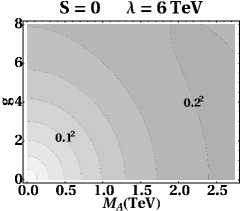
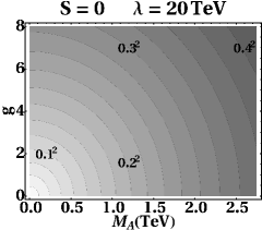
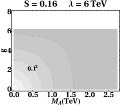
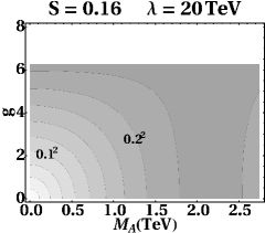
Figure 1: Contour plots of $m^{2}_{\mathrm{walk}}$ as function of $M_{A}$ and $g=M_{V}^{2}/(\sqrt{2}F_{V})$ for $S=0$ ($S=S_{\mathrm{pert}}^{\mathrm{MWT}}\approx 0.16$) and $\lambda=6$TeV ($\lambda=20$ TeV). Contours are for $m^{2}_{\mathrm{walk}}=0.025^{2}$ TeV², $0.05^{2}$ TeV², $0.075^{2}$ TeV², …with zero at the origin. For $S=S_{\mathrm{pert}}^{\mathrm{MWT}}$, the plot range in $g$ is constrained by the requirement $F_{A}^{2}>0$.

Apart from imposing the first Weinberg sum rule we introduce a coupling $g$ in the spirit of the coupling connected to a local symmetry such that $M_{V}^{4}=2g^{2}F_{V}^{2}$. It is expected to be of order unity. For positive $S$ there is an upper limit for $g$ above which $F_{A}^{2}$ turns negative. In the plots, we display $m^{2}_{\mathrm{walk}}$ which is a model independent factor. The detailed mass structure $\hat{m}^{2}_{ab}$ differs between models. The normalisation of $m^{2}_{\mathrm{walk}}$ has been chosen such that the eigenvalues of $\hat{m}^{2}_{ab}$ are in general of order unity. Hence, one can directly gain an initial impression on the magnitude of the pion masses from the numbers in the plots in Fig. 1: For small $S$ parameters and large values of $\lambda$, $M_{A}$ and $g$ up to 400GeV can be reached, which corresponds to five times the mass of the W boson.

For a concrete model, MWT features two techniquarks transforming under the adjoint representation of an $SU(2)$ gauge group. The adjoint representation is real. The unbroken chiral symmetry is therefore enhanced to $SU(4)$ which breaks to $SO(4)$ yielding nine Goldstone modes, three of which become the longitudinal degrees of freedom of the weak gauge bosons. This leaves behind six extra technipions which here carry nonzero baryon number. In this setup, the techniquarks alone would lead to a theory with a global Witten anomaly, as an odd number of fermions [The adjoint of $SU(2)$ is three-dimensional.] would transform under the $SU(2)_{L}$ of the Standard Model. The anomaly is cancelled by including an additional pair of leptons. Due to the presence of these leptons the requirement of freedom from gauge anomalies does not fix the hypercharge assignment completely, but leaves one free continuous parameter.

By using the generators of MWT from Dietrich:2005jn ; Foadi:2007ue in (9) we find for the electroweak contributions to the masses of the technipions of MWT which are not eaten by the electroweak gauge fields,

$$\left(g_{1}^{2}+g_{2}^{2}\right)\hat{m}^{2}_{\Pi_{UU}} = g_{1}^{2}\left(1+2y\right)^{2}+g_{2}^{2}$$

$$\left(g_{1}^{2}+g_{2}^{2}\right)\hat{m}^{2}_{\Pi_{DD}} = g_{1}^{2}\left(1-2y\right)^{2}+g_{2}^{2}$$

$$\left(g_{1}^{2}+g_{2}^{2}\right)\hat{m}^{2}_{\Pi_{UD}} = g_{1}^{2}\left(4y^{2}-1\right)+g_{2}^{2}.$$ (20)

Here $y$ is a parameter that controls the hypercharge assignment of the techniquarks and the subscripts $U$ and $D$ denote the flavours of the techniquarks which constitute the corresponding technipion. The masses of the charge conjugate pions are the same. Since $g_{2}>g_{1}$ the squared masses are positive for all values of $y$. In Table 1 we present the numerical values for the most natural choices of $y$. $g_{1}$ and $g_{2}$ are weakly dependent on the mixing of the electroweak gauge bosons with the composite vector states in MWT. We use their standard model (tree-level) values which is sufficient for our purposes.

$$\begin{array}[]{c||ccc}y&\quad\hat{m}^{2}_{\Pi_{UU}}&\quad\hat{m}^{2}_{\Pi_{DD}}&\quad\hat{m}^{2}_{\Pi_{UD}}\\ \hline\cr\hline\cr 0&\quad 1&\quad 1&\quad 0.53\\ +1&\quad 2.87&\quad 1&\quad 1.47\\ -1&\quad 1&\quad 2.87&\quad 1.47\end{array}$$ (25)

Table 1: Eigenvalues of $\hat{m}_{ab}^{2}$ for the uneaten technipions in MWT for various values of the parameter $y$.

The squares of the physical masses as functions of $M_{A}$ and $g$ are obtained by multiplying the values in Fig. 1 by the factors of Table 1. Pion masses for the light mass window Foadi:2007ue of MWT, where $M_{A}<M_{V}\lesssim 1$ TeV, are from 50 to 300 GeV. For the heavy mass window, where $M_{A}>M_{V}\gtrsim 2$ TeV, all pion masses are at least 150 GeV. Interestingly, the pion masses can be large enough to exceed present experimental bounds even without any additional extended technicolour (ETC) interactions, expect in the region of small $M_{A}$ and $g$.

The low-energy limit of the continuum is given by twice the dynamical mass $\Sigma(0)$, i.e., the threshold of the loop. It’s estimated to be $2\Sigma(0)\approx 4\pi f_{\pi}/d_{\mathrm{R}}$. For MWT this evaluates to circa 1 TeV. Picking resonances considerably above this value entails a slight modification of the picture, if one does not want to put them inside the continuum: The continuum threshold has to be taken higher. The only definite constraint for our investigation is that the scale $\lambda$ must lie inside the continuum. As we have chosen reference values of $\lambda=6$ TeV and $\lambda=20$ TeV, we extend our plots to close to 3 TeV resonance masses.

The model known under the name Next-to-Minimal Walking Technicolour (NMWT) possesses two techniquarks which transform under the two-index symmetric representation of SU(3) which is not (pseudo)real, but even-dimensional. Consequently, the flavour symmetry breaking pattern is $SU(2)_{L}\times SU(2)_{R}\rightarrow SU(2)_{V}$ leading to three Goldstone modes which are all eaten by the weak gauge bosons. Hence, there are no degrees of freedom left which would receive contributions to their mass in the framework of the present analysis.

Other viable candidates for dynamical electroweak symmetry breaking by walking TC theories are discussed in Dietrich:2006cm and can be analysed using the above formulae.

Summary. We studied the modifications of the Weinberg sum rules in quasiconformal gauge field theories. We showed that while the $X$ parameter is not directly altered by nearly conformal dynamics, the electroweak corrections to pion masses can be enhanced considerably wrt. running theories. As an explicit example we discussed MWT where the typical scale of these corrections was seen to be from 100 to 200 GeV. Interestingly, the technipion masses can be large enough to exceed present experimental bounds even without any additional ETC interactions, expect in the region of small $M_{A}$ and $g$.

The naive expectation that the masses (not the squared masses) at least in the running case can be simply scaled up from their value in quantum chromodynamics to their value in techincolour by the ration say of the respective pion decay constants is not confirmed. For the QCD pions the above formulation returns the difference if the squared masses of the charged and the neutral pions. In order to obtain the linear mass difference, the result has to be divided by the sum of the masses, which is dominated by explicit symmetry breaking, i.e., the bare quark masses. In the application to TC directly the squared masses of the uneaten pions are computed, the square root of which returns the linear masses. Therefore, it is understandable that the thus obtained pion masses may (and do) exceed the values obtained by scaling up the QCD masses. Quasiconformal dynamics leads to an additional enhancement.

Acknowledgments. The authors acknowledge useful discussions with Roshan Foadi, Mads T. Frandsen, Chris Kouvaris, and Francesco Sannino. The work of DDD was supported by the Danish Natural Science Research Council. The work of MJ was supported by the Marie Curie Excellence Grant under contract MEXT-CT-2004-013510.

References

- (1) S. Weinberg, Phys. Rev. D 19, 1277 (1979); L. Susskind, Phys. Rev. D 20, 2619 (1979).
- (2) B. Holdom, Phys. Rev. D 24, 1441 (1981); K. Yamawaki, M. Bando and K. i. Matumoto, Phys. Rev. Lett. 56, 1335 (1986); T. W. Appelquist, D. Karabali and L. C. R. Wijewardhana, Phys. Rev. Lett. 57, 957 (1986); V. A. Miransky and K. Yamawaki, Phys. Rev. D 55, 5051 (1997) [Erratum-ibid. D 56, 3768 (1997)] [arXiv:hep-th/9611142]; V. A. Miransky, T. Nonoyama and K. Yamawaki, Mod. Phys. Lett. A 4, 1409 (1989); K. D. Lane and E. Eichten, Phys. Lett. B 222, 274 (1989); E. Eichten and K. D. Lane, Phys. Lett. B 90, 125 (1980).
- (3) D. D. Dietrich, F. Sannino and K. Tuominen, Phys. Rev. D 73 (2006) 037701 [arXiv:hep-ph/0510217]; Phys. Rev. D 72 (2005) 055001 [arXiv:hep-ph/0505059]; F. Sannino and K. Tuominen, Phys. Rev. D 71 (2005) 051901 [arXiv:hep-ph/0405209].
- (4) D. D. Dietrich and F. Sannino, Phys. Rev. D 75 (2007) 085018 [arXiv:hep-ph/0611341]; T. A. Ryttov and F. Sannino, Phys. Rev. D 78 (2008) 065001 [arXiv:0711.3745 [hep-th]]; T. A. Ryttov and F. Sannino, Phys. Rev. D 78, 115010 (2008) [arXiv:0809.0713 [hep-ph]]; F. Sannino, arXiv:0811.0616 [hep-ph].
- (5) S. B. Gudnason, C. Kouvaris and F. Sannino, Phys. Rev. D 73, 115003 (2006) [arXiv:hep-ph/0603014]; Phys. Rev. D 74 (2006) 095008 [arXiv:hep-ph/0608055]. D. D. Dietrich and C. Kouvaris, arXiv:0805.1503 [hep-ph]; arXiv:0809.1324 [hep-ph]; A. Belyaev, R. Foadi, M. T. Frandsen, M. Järvinen, F. Sannino and A. Pukhov, arXiv:0809.0793 [hep-ph].
- (6) R. Foadi, M. T. Frandsen, T. A. Ryttov and F. Sannino, Phys. Rev. D 76 (2007) 055005 [arXiv:0706.1696 [hep-ph]]; R. Foadi, M. T. Frandsen and F. Sannino, arXiv:0712.1948 [hep-ph]; R. Foadi and F. Sannino, arXiv:0801.0663 [hep-ph]; R. Foadi, M. Järvinen and F. Sannino, arXiv:0811.3719 [hep-ph].
- (7) S. Weinberg, Phys. Rev. Lett. 18 (1967) 507.
- (8) T. Appelquist and F. Sannino, Phys. Rev. D 59 (1999) 067702 [arXiv:hep-ph/9806409].
- (9) M. E. Peskin and T. Takeuchi, Phys. Rev. Lett. 65 (1990) 964.
- (10) T. Das, G. S. Guralnik, V. S. Mathur, F. E. Low and J. E. Young, Phys. Rev. Lett. 18 (1967) 759.
- (11) M. E. Peskin, Nucl. Phys. B 175 (1980) 197.
- (12) R. Barbieri, A. Pomarol, R. Rattazzi and A. Strumia, Nucl. Phys. B 703 (2004) 127 [arXiv:hep-ph/0405040].