1]Space Science Center, University of New Hampshire, Durham, New Hampshire, 03824 2]Department of Physics and Astronomy, State University of New York, Stony Brook, New York, 11794 3]Department of Physics, Applied Physics and Astronomy, Rensselaer Polytechnic Institute, Troy, New York, 12180 4]University Joseph Fourier – Grenoble I, BP 53, 38041 Grenoble Cedex 9, France 5]Laboratoire des Ecoulements Géophysiques et Industriels, CNRS/UJF/INPG UMR 5519 BP53, 38041 Grenoble, France
John Podesta
(jpodesta@solar.stanford.edu)
Accurate estimation of third-order moments from turbulence measurements
Zusammenfassung
Politano and Pouquet’s law, a generalization of Kolmogorov’s four-fifths law to incompressible MHD, makes it possible to measure the energy cascade rate in incompressible MHD turbulence by means of third-order moments. In hydrodynamics, accurate measurement of third-order moments requires large amounts of data because the probability distributions of velocity-differences are nearly symmetric and the third-order moments are relatively small. Measurements of the energy cascade rate in solar wind turbulence have recently been performed for the first time, but without careful consideration of the accuracy or statistical uncertainty of the required third-order moments. This paper investigates the statistical convergence of third-order moments as a function of the sample size . It is shown that the accuracy of the third-moment depends on the number of correlation lengths spanned by the data set and a method of estimating the statistical uncertainty of the third-moment is developed. The technique is illustrated using both wind tunnel data and solar wind data.
1 Introduction
In the solar wind, coupling between large- and small-scale turbulence occurs at kinetic scales defined by the ion gyro-radius and the ion gyro-period. At these scales, the turbulent energy cascade undergoes a transition from large magnetohydrodynamic (MHD) scales to small plasma kinetic scales where the energy is ultimately dissipated by collisionless processes. Detailed understanding of the energy cascade process at MHD-scales is a prerequisite for studies of this coupling. Here we focus on one particular aspect of MHD-scale turbulence which is of some practical importance, namely, the determination of the energy cascade rate from measured data.
MHD-scale turbulence in the solar wind is often modeled using the theory of incompressible MHD because of its relative simplicity, even though the solar wind is known to be compressible. In the solar wind, the energy density of MHD turbulence is comparable to the plasma thermal energy at 1 AU (Belcher and Davis, 1971) and the turbulent energy cascade is believed to significantly heat the solar wind plasma as it flows from AU to several tens of AU. Theoretical work has shown that plasma heating caused by dissipation of the turbulence can likely explain the observed radial temperature profile of the solar wind which decreases more slowly than would be the case if the expansion were adiabatic (Matthaeus et al., 1996; Zank et al., 1999; Matthaeus et al., 1999; Smith et al., 2001; Isenberg et al., 2003). To refine these theories, accurate measurements of the energy cascade rate are needed. Recently, the energy cascade rate has been directly measured for the first time in the solar wind using a generalization of Kolmogorov’s four-fifths law (MacBride et al., 2005; Sorriso-Valvo et al., 2007; MacBride et al., 2008; Marino et al., 2008). Before discussing this, it may be helpful to provide some background information on Kolmogorov’s four-fifths law.
For turbulent flows in ordinary incompressible fluids such as air or water the energy cascade rate is often measured indirectly by means of the energy dissipation rate
| (1) |
where is the kinematic viscosity and the coefficient 15 arises from the assumption that the turbulence is isotropic (Pope, 2000, p. 134). The energy cascade rate can also be measured directly by means of Kolmogorov’s four-fifths law
| (2) |
valid for isotropic turbulence, where
| (3) |
is the component of the velocity fluctuation in the direction of the displacement and the lengthscale lies in the inertial range (Kolmogorov, 1991; Frisch, 1995). Note that Kolmogorov’s four-fifths law (2) is independent of the kinematic viscosity and can be applied even when the kinematic viscosity is unknown, but the accurate evaluation of the third-order moment (2) requires much more data than the second-order moment (1).
Kolmogorov’s four-fifths law was originally derived for homogeneous isotropic turbulence and a similar law was later derived by Monin for homogeneous anisotropic turbulence; see Podesta et al. (2007) for references. Politano and Pouquet (1998a, b) generalized these fundamental results of Kolmogorov and Monin from the theory of incompressible hydrodynamic turbulence to incompressible MHD turbulence. It is important to emphasize that Politano and Pouquet’s law holds for both isotropic and anisotropic turbulence, although this fact was not explicitly mentioned by Politano and Pouquet (1998a). This is especially important in MHD where statistical isotropy may not hold in the presence of an ambient magnetic field. A derivation of Politano and Pouquet’s law which is similar to Frisch’s derivation of Kolmogorov’s four-fifths law is given by Podesta (2008).
Politano and Pouquet’s law has recently been applied to obtain direct measurements of the energy cascade rate in the solar wind under the simplifying assumption that the turbulence is isotropic (MacBride et al., 2005; Sorriso-Valvo et al., 2007; MacBride et al., 2008; Marino et al., 2008). MacBride et al. (2008) have also investigated a non-isotropic 1D/2D hybrid model that is believed to be descriptive of the solar wind. The method used in all these studies consists of the evaluation of certain third-order moments which are similar to those in equation (2), except that for incompressible MHD turbulence the relevant third-order moments contain combinations of velocity and magnetic field fluctuations (or, equivalently, fluctuations in the Elsasser variables). From the linear scaling of these third-order moments, the energy cascade rate is obtained without any knowledge of the dissipation processes or the viscous and resistive dissipation coefficients in the the solar wind.
The solar wind studies mentioned above have not given careful consideration to the convergence properties of third-order moments which raises the question: how much data is required to accurately estimate the third-order moments? The study by Sorriso-Valvo et al. (2007) used approximately 2000 data points to compute the third-order moments while the study by MacBride et al. (2008) used close to data points. The purpose of the present work is to investigate the accuracy of third-order moments as a function of the sample size (the number of data points used in the analysis). An important conclusion is that the accuracy of third-order moments depends on the number of correlation lengths spanned by the data set (defined below). The number of correlation lengths determines the accuracy and statistical uncertainty of third-order moments computed from measured data, not the number of data points . It turns out that for turbulence studies where the skewness of the distribution is usually small the accurate estimation of third-order moments requires large amounts of data. The reason is partly because the third moment is not an absolute moment but a signed moment and, therefore, is subject to cancellation effects. The theory describing the convergenge of these moments is illustrated using turbulence data from the ONERA/Modane wind tunnel. The same techniques can be applied to third-order moments in solar wind turbulence which exhibit similar behavior.
2 Theory
2.1 Uncorrelated time series
Given independent samples drawn randomly from a probability distribution , the moments of the distribution can be estimated as
| (4) |
| (5) |
| (6) |
etc. Now focus attention on the third moment and let
| (7) |
Note that is itself a random variable whose probability distribution can be derived, in principle, from the pdf of the random variable . Now suppose that we know the mean and standard deviation of the random variable denoted by and , respectively. If , then for to be an accurate estimate of the standard deviation must be small compared to the mean, that is,
| (8) |
This condition can be used to estimate the sample size required to obtain an accurate estimate of the third moment. Hereafter, it is assumed that .
From equation (7) and the independence of the , the first and second moments of are
| (9) |
and
| (10) |
Thus, the variance is
| (11) |
and
| (12) |
The value of required to make the last equation small depends on the ratio and, therefore, depends on the distribution function . If the ratio is on the order of unity, then may be adequate. But, if this ratio is much larger than unity, then will have to increase accordingly. The relation (12) shows that to increase the accuracy of the third-moment by a factor of ten requires an increase in the sample size by a factor of 100. This slow rate of convergence imposes practical limitations on estimates of third-order moments obtained from experimental data.
2.2 Correlated time series
For applications to turbulence, the random variable is a velocity difference such as and the sequence is usually not mutually stochastically independent. For example, two velocity increments that overlap in space or time are usually correlated to some degree. In this case, the number of “independent samples” in the above theory should be replaced by the number of correlation lengths of the quantity under consideration. For the third-order moment it is necessary to use the correlation length or correlation time of the time series and replace in equation (12) by the number of correlation lengths
| (13) |
where is the temporal record length and is the sampling time. Thus, equation (12) takes the modified form
| (14) |
or, equivalently,
| (15) |
where . Note that this is almost the same as equation (12) except for an additional scale factor . Because the correlation times of the sequences and can be different it is important to use the correlation time of the sequence in equations (13)–(15) when analyzing the third-order moment.
3 Textbook example
An example is now given to illustrate the theory described in section 2. Consider the slightly skewed distribution function
| (16) |
where the parameter characterizes the skewness of the distribution. The distribution has zero mean, , and reduces to the Gaussian distribution when . If , the pdf of is
| (17) |
The moments of the distribution function (17) can be computed from the characteristic function
| (18) |
by means of the well known relations
| (19) |
etc. After some tedious calculations, the first six moments are found to be
| (20) |
Thus, from the relation , the first six moments of the variable are
| (21) |
For the particular distribution function (16), the ratio (12) takes the form
| (22) |
For , for example, this becomes
| (23) |
This ratio is small if . In this idealized example where the distribution function is known, the number of samples required to obtain an accurate estimate of the third moment from experimental data can be computed explicitly. For turbulence data acquired in the laboratory, such precise estimates cannot be computed a priori because the distribution function is unknown.
4 A practical approach
When working with experimental turbulence data the distribution function is usually unknown so that the ratio in equation (12) cannot be evaluated. A practical approach is to compute the third-moment from the data and then construct the empirical distribution function for , where is now fixed (a constant). This too may be impractical because of the large number of data points required. However, the distribution function for contains more information than is needed. Just a few independent estimates of the third-moment , perhaps 10, may be sufficient to obtain a rough estimate of the ratio in equation (8). The number of samples can then be increased until the ratio so obtained satisfies the inequality (8). This is a simple way of controlling the accuracy of third-order moments estimated from turbulence measurements. The effectiveness of the method can be improved by increasing the number of independent estimates of used to compute the mean and standard deviation. The standard deviation obtained from the data provides a rough estimate of the 1- error for the third-order moment.
A more precise analysis can be performed by computing histograms, means, and standard deviations of the third-moment for progressively larger values of . Accurate values of the mean and standard deviation can be obtained for values of much smaller than the record size. Fitting the measured ratio to the functional form , where is an adjustable parameter, it is then possible to extrapolate the ratio to larger where direct calculations have poor statistics or are unattainable as a consequence of the limited record size. An alternate fitting function is where and are two adjustable parameters. From this extrapolation it is possible to determine the value of the sample size required to achieve any desired accuracy of the ratio and, therefore, of the third-order moment . This approach is accurate and effective as long as sufficient data are available and requires no apriori knowledge of the distribution function or its moments. The same technique can also be applied to accurately determine moments of any order provided sufficient data are available.
5 Illustration using wind tunnel data
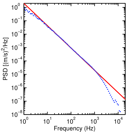
The technique described in the previous section shall now be applied to study turbulence data from the ONERA wind tunnel in Modane, France, characterized by a Taylor-scale Reynolds number (Kahalerras et al., 1998; Malécot et al., 2000; Gagne et al., 2004). This particular data set is a time series consisting of data points with a sampling rate of 25 kHz and an average velocity of 20.37 m/s. The inertial range extends from Hz to Hz as inferred from the power spectrum shown in Figure 1.
Now, consider the third-order moment
| (24) |
where s or, equivalently, Hz. This time lag is chosen for study because it lies inside the inertial range displayed in Figure 1.
The third-order moment is computed using a contiguous series of N data points. A set of N contiguous data points is called a data block. A series of successive data blocks are then used to compute a series of third-order moments, one for each data block. The first data point in a given data block is separated from the first point of the next successive data block by an offset where, ideally, . When the sample size is not small compared to the record size, smaller values of the offset are used so that the total number of data blocks yields a sufficient statistical sample. Note, however, that when the offset is smaller than the third-order moments obtained from successive data blocks become dependent (because the blocks overlap) and, consequently, to obtain good statistics it is advisable not to let become much smaller than . This tradeoff is unavoidable when working with records of finite length.
The set of third-order moments obtained for a given sample size are used to generate a histogram of third-order moments as shown in Figure 2.
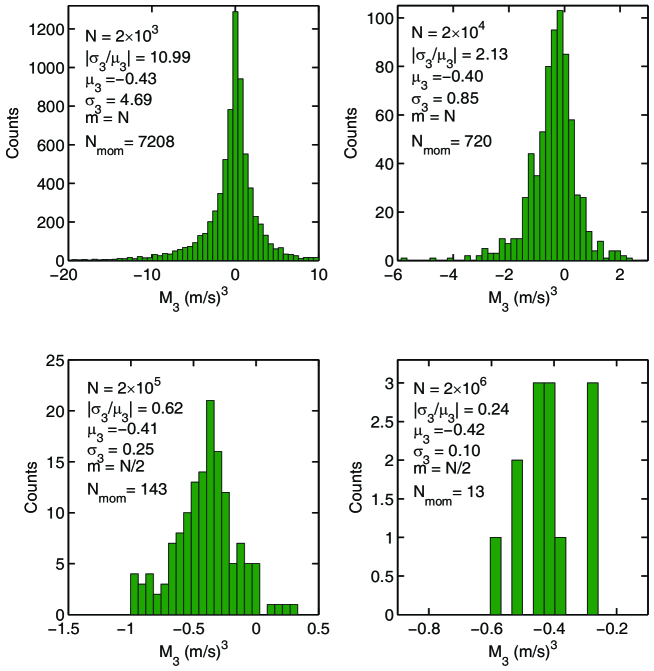
The number of third-order moments is equal to the number of data blocks employed in the calculation. As expected, the width of the distributions as measured by the standard deviation is a decreasing function of . Moreover, the results for the ratio of the standard deviation to the mean are in approximate agreement with the convergence rate predicted by the theory in section 2. Thus, increasing by a factor of ten causes a decrease in the ratio of the standard deviation to the mean by a factor of .
The third-order moment obtained using all available data is (m/s)2. Note that the mean displayed in Figure 2 is approximately independent of . This is to be expected because for any sequence of numbers partioned into successive non-overlapping blocks, the average of the mean values for each data block is equal to the mean value of the entire record. In practice, the data blocks may not completely cover the given record because the record size is not divisible by and, therefore, the equality is only approximate. This explains the approximate independence of versus in Figure 2. See also equations (9) and (11) which predict that is independent of and .
How much data is required to obtain an accurate estimate of the third-order moment? This depends, of course, on the level of error which is tolerable for the application at hand. The relative error is measured by the ratio . This quantity is plotted as a function of in Figure 3 (upper plot).
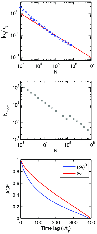
To ensure a reasonably large number of third-moments , the offset between successive data blocks is when and when . The number of third-moments is shown in the middle plot in Figure 3. The theoretical relation (15) takes the form
| (25) |
where the value 304 is obtained using the empirical values of the sixth moment (m/s)6, the third moment (m/s)6, and the correlation time defined as the time where the autocorrelation function equals 1/2 (Figure 3). Inspection of the theoretical curve, the red line in Figure 3, shows that to achieve the level of precision would require data points or, equivalently correlation lengths. The total number of data points contained in the data set is .
One can see from this example that accurate estimation of third-order moments from turbulence data requires a very large record length. Under circumstances where sufficiently large data sets are not available, the techniques described here and in the last section can be used to estimate the errors in the third-moment as quantified by the standard deviation and the empirical ratio .
So far in this section the analysis of the third-moment has been carried out for one time lag s. The same analysis can be carried out for many different time lags and, in this case, the error is typically an increasing function of time lag throughout the inertial range (for a fixed sample size ). The third-order moment as a function of the time lag computed using all available data is shown in the upper plot in Figure 4. For the data shown in Figure 4,
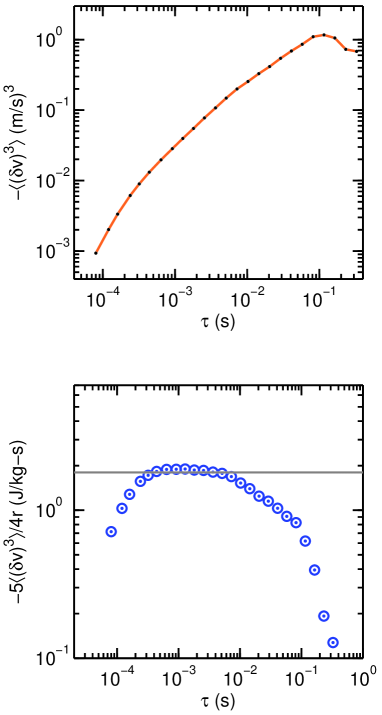
estimates show that the relative error lies approximately in the range for s and for s. Hence, the third-moments are sufficiently accurate for the present purpose only for s.
To estimate the energy cascade rate using Kolmogorov’s four-fifths law (2), the quantity is plotted versus in the lower panel in Figure 4. Note that compressibility effects are negligible because the Mach number is much less than unity and, therefore, the application of Kolmogorov’s four-fifths law is justified. In the lower panel in Figure 4, the data lie approximately on the horizontal line J/kg-s throughout the range s. Thus, the value of the energy cascade rate determined by Kolmogorov’s four-fifths law is J/kg-s. Note that the range s where where an apparent plateau is formed does not coincide with the inertial range s inferred from Figure 1. Because the dissipation range lies just beyond the spectral break near Hz in Figure 1 (Pope, page 237), this implies that the region where the four-fifths law holds includes part of the dissipation range. It is also puzzling why the four-fifths law breaks down for s in Figure 4 since the inertial range appears to extend to s in Figure 1. Consequently, Kolmogorov’s four-fifths law does not hold throughout the entire inertial range as the theory seems to predict. The reason for these discrepancies is unknown at the moment. However, results for the scaling of the third-order moment in Figure 4 are in agreement with Gagne et al. (2004) who analyzed the same Modane data.
An independent estimate of the energy cascade rate is obtained using equation (1). If the measured signal is approximated by the truncated Fourier series
| (26) |
where is the record length, , and is the sampling time, then the time average of is given by
| (27) |
where
| (28) |
is the discrete Fourier transform of the sequence which is easily evaluated using the FFT. Using the entire data record to evaluate (27) and the value m2/s, the energy dissipation rate obtained from equation (1) is J/kg-s.
The spatial separation between two consecutive measurements mm is roughly three times the Kolmogorov scale mm; the normalized wavenumber is . Because most of the dissipation occurs in the wavenumber range (Pope, 2000, p. 237, Fig. 6.16), estimates of from the Modane data should be accurate. (Although Fig. 6.16 in Pope’s book is drawn for the case , a similar plot in the case is almost indistinguishable from the case .) Note that the value of given in Table 1 of Malécot et al. (2000) is in error, the correct value is given in Yann Malécot’s thesis and also in Kahalerras et al. (1998) and in Gagne et al. (2004) where the same Modane data is used.
In summary, it has been shown that the energy cascade rate J/kg-s obtained by Kolmogorov’s four-fifths law is in rough agreement with the energy dissipation rate J/kg-s obtained from equation (1).
6 Illustration using solar wind data
In this section, we present two examples to illustrate the convergence of third-order moments for solar wind data. The first example uses 1 second data for the radial magnetic field component measured above the poles of the sun by the Ulysses spacecraft. The second example uses 64 second data for the radial solar wind velocity measured in the ecliptic plane near 1 AU by the ACE spacecraft.
6.1 Analysis of using Ulysses data
The radial magnetic field component (in spacecraft RTN coordinates) was chosen because it enters the third-moment that appears in the law for the cross-helicity cascade in MHD turbulence (Podesta et al., 2007; Podesta, 2008). Ulysses data was chosen because it is devoid of magnetic sector crossings which are usually present in data acquired near the ecliptic plane. The third-moment changes algebraic sign in outward and inward magnetic sectors. For this reason, the presence of different magnetic sectors significantly complicates the analysis of this third-order moment.
The Ulysses data selected for analysis consists of a time series of s data from the vector-helium magnetometer (Balogh et al., 1992) spanning the time interval from 1 July 1994 to 1 October 1994, 92 days. During this time Ulysses distance from the sun decreased from 2.80 AU to 2.17 AU as its heliographic latitude remained between and degrees. The reversal of the solar magnetic field in the southern hemisphere was completed in 1992 (Snodgrass et al., 2000) so the data used here contains only one magnetic sector. The time tags on the data show some data have a 1/2 second cadence, some data have a 1 or 2 second cadence, and there are also data gaps of various sizes. The 1/2 sec data is downsampled to 1 sec and the data gaps are left intact to create a time series with a uniform cadence of 1 sec. Times when data are missing are marked with fill values (such data are easily omitted from the analysis). There are a total of data points in the time series and 23.55% of these points are missing data markers (fill values). The average value of for the entire time series is nT.
The power spectrum for the Ulysses data shown in Figure 5 is strikingly similar to that of the wind tunnel data in Figure 1.
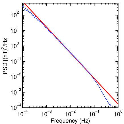
From Figure 5, the inertial range appears to extend from less than Hz to approximately Hz. The time lag seconds or, equivalently, Hz is chosen for analysis because it lies inside the inertial range. The same procedures used to analyze the Modane data are employed for the Ulysses data except that missing data is excluded from the analysis. Consequently, a data block of size contains less than samples (because of the presence of fill values) and the actual number of samples varies from block to block. Only those data blocks where are included in the analysis and the average number of samples taken over all blocks of a given size is defined to be the sample size for that run.
The results of the statistical analysis of Ulysses data for the time lag seconds are shown in Figure 6.
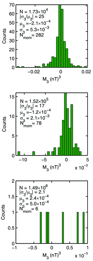
The sizes of the data blocks used in the analysis are , , and . The offset from one data block to the next is for the upper plot and for the other two plots. The algebraic sign of is negative except in the lower plot, however, the sample size in the lower plot is too small to yield adequate statistics. The value of the third-moment obtained using the entire data record is (nT)3, a very small value. To gain some idea of the error, the error of the mean estimated from Figure 6 is roughly (nT)3.
The theoretical relation (15) may be evaluated using estimates obtained from the data for the third-moment (nT)3, the sixth-moment (nT)6, and the correlation time s determined from the autocorrelation function for the sequence . The values of the moments are uncertain, especially higher order moments such as which can be strongly affected by the presence of outliers in the data (Horbury and Balogh, 1997), however, they are used anyway to explore the fit to the data of the relation (15). Thus, the theoretical relation (15) takes the form
| (29) |
For the three runs shown in Figure 6 the theoretical values for the ratio are 57, 19, and 6. These are roughly consistent with the values found in Figure 6. For all data, and the relation (29) predicts a relative errror . Hence, (nT)3, which is consistent with the estimates in the preceeding paragraph.
In summary, the large magnitude of the ratio is partly due to the fact that is close to zero and this makes it impossible to obtain adequate convergence with the limited data used in this study. One may conclude from these results that a much larger data set than the one used here is needed to determine the third-moment of accurately. Nevertheless, the results presented here are still useful for determining approximate upper and lower bounds for this third-order moment.
6.2 Analysis of using ACE data
Solar wind measurements of the radial velocity component from the Advanced Composition Explorer (ACE) are analyzed in the same way. The ACE spacecraft is in orbit around the Sun-Earth libration point sunward of the Earth. The ACE SWEPAM plasma instrument has a 64-second cadence (McComas et al., 1998) and we use all data available during the three year period from 2005 through 2007, about 1.4 million data points. Note that solar minimum is expected to occur in late 2008 or early 2009. Non-overlapping data blocks of 100 points (about 10,000 blocks) to 256,000 data points (5 blocks) are used. Each data block may include fill values (missing data markers) that are present in the time series. All fill values are omitted from the analysis and any data block in which the number of fill values exceeds 10% is excluded from analysis. Third-order moments of are calculated for two different time lags, seconds and seconds. The inertial range in the ecliptic plane near 1 AU extends from about 1 second to about 1 hour and, therefore, both of these time lags lie in the inertial range.
Figure 7
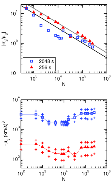
shows that in the solar wind, the ratio of the standard deviation of the third-moment to the average value of the third-moment has the same dependence predicted by equation (15) as does the wind tunnel data analyzed in Section 5. Remarkably, the amplitude of this relation is quantitatively similar for both wind tunnel data and solar wind data, even though the solar wind has a fast/slow stream structure and the turbulence is magnetohydrodynamic in nature. As with the wind tunnel data, it appears from Figure 7 that more than solar wind velocity measurements are needed to accurately determine the third-order moment (error less than 10%). However, sample sizes may give sufficient accuracy for some applications.
Also plotted in the upper plot in figure 7 are the theoretical curves, equation (15), for the two time lags studied. A rough estimate of equation (15) is obtained by using all data in the record to estimate the sixth-moment of , , the third-moment , and the correlation time of the sequence . For the time lag s, this yields (km/s)6, (km/s)3, and . In this case, and equation (15) becomes
| (30) |
For the time lag s, (km/s)6, (km/s)3, and . In this case, and equation (15) becomes
| (31) |
These represent reasonable asymptotic fits to the data shown in Figure 7 as becomes large.
What accuracy can be claimed for measurements of this third-order moment in the solar wind? The upper plot in Figure 7 indicates that for data points the error is around . The lower plot in Figure 7 shows the mean values of the third moment plus and minus the standard error of the mean , where is the number of moments used to compute the mean. It appears that the relative error is roughly the same at both lags and that within the calculated errors the third moment is proportional to lag. Such proportionality is most clearly demonstrated by computing the third-moment as a function of the time lag (not shown).
It is interesting that both wind tunnel data and solar wind velocity data require roughly the same number of data points to obtain good convergence of third-order moments for time lags in the inertial range. In part, this may be because both kinds of turbulence have similar Reynolds numbers. The Reynolds number in the solar wind can crudely be estimated using the hydrodynamic relation , where is the integral scale, is the Kolmogorv scale (dissipation scale), and Re is the Reynolds number based on the integral scale. Solar wind power spectra indicate that and, therefore the Reynolds number is of order . This is equivalent to a Taylor-scale Reynolds number
| (32) |
(Pope, 2000, p. 200, eqn. 6.64). Thus, the Reynolds numbers of Modane wind tunnel data and solar wind velocity data at 1 AU are similar.
7 Conclusions
The purpose of this study is not to compute turbulent energy cascade rates using third-order moments. The purpose of this study is to show how the accuracy of third-order moments can be estimated and controlled. A simple theory is presented that describes the statistical convergence of third-order moments, such as , as a function of the record length. An important conclusion is that the accuracy of third-order moments depends on the number of correlation lengths spanned by the time series as expressed by equations (14) and (15). The techniques described here are useful for assessing the accuracy of third-order moments obtained using measured data. Practical applications of the theory have been illustrated using wind tunnel data and solar wind data.
For the accurate calculation of third-order moments from wind tunnel data with a Taylor-scale Reynolds number , the number of data points required to obtain an error less than 10% at the time lag ms is or, equivalently, a record length spanning correlation lengths. For fluctuations of the radial solar wind velocity , the analysis of ACE data in the ecliptic plane near 1 AU shows that for the time lags s and s the number of data points required for an accurate determination of the third-order moment is also roughly . This is equivalent to and correlation lengths for s and s, respectively. However, data points may yield sufficient accuracy for some applications.
For fluctuations of the radial magnetic field component over the poles of the sun at a heliocentric distance of approximately 2.5 AU, the value of the third-order moment is close enough to zero that convergence of the third moment could not be demonstrated using an interval of Ulysses data with approximately six million points (not including fill values), a record consisting of approximately correlation lengths. This suggests that third-order moments of solar wind magnetic field components must be computed carefully because without a sufficiently large number of data points and without evaluation of the probable errors using eq (15) the calculation of the third-order moments are not meaningful.
It should be noted that the above two examples based on solar wind data from Ulysses and ACE are distinctly different from each other and from the example based on Modane wind tunnel data. The Ulysses study pertains to the radial magnetic field component at high heliographic latitudes and the ACE study pertains to the radial velocity component in the ecliptic plane. These studies provide two separate examples of the estimation of third-order moments and their uncertainties using solar wind data. For wind tunnel data, Kolmogorov’s four-fifths law predicts the third-order velocity moment scales linearly in the inertial range. For solar wind data, neither the third-order moment of the radial velocity component nor the third-order moment of the radial magnetic field component is predicted to scale linearly. The latter examples simply serve to illustrate the application of statistical convergence techniques to solar wind data. It is of interest to note, however, that the third-order moment of the radial velocity component in the solar wind was found to scale approximately linearly in the study by MacBride et al. (2008) and appears to provide the dominant contribution to the energy cascade rate estimated from the scaling relations of Politano and Pouquet (1998).
In conclusion, the present study has some noteworthy implications for measurements of the energy cascade rate in the solar wind. Empirical estimates of the energy cascade rate in the solar wind have recently been obtained under the assumption that the turbulence is approximately incompressible and isotropic so that the third-moment scaling relations of Politano and Pouquet (1998) for homogeneous isotropic incompressible MHD turbulence could be applied. In the studies by Sorriso-Valvo et al. (2007) and Marino et al. (2008) the number of data points employed to compute the required third-order moments was around 2000. As shown in the present study, this number is insufficient to obtain accurate estimates of third-order moments in the solar wind. This may explain why Sorriso-Valvo et al. (2007) and Marino et al. (2008) did not find a linear scaling of the third-order moments in some of the intervals they studied, and why they found it was rare for linear scaling to be observed simultaneously for both of the Elsasser variables. Although MacBride et al. (2008) did not use the convergence tests proposed here, they used large enough data sets that the third order moments in the Politano and Pouquet scaling laws became insensitive to adding more data. To obtain stable estimates of the third-moments, this convergence criterion required the use of at least one year of ACE plasma and magnetic field data, roughly data points. In the future, the convergence of third-order moments and the associated error estimates that such convergence studies provide should become an integral part of any analysis of solar wind data involving third-order moments.
Acknowledgements.
We are grateful to Bernard Vasquez for helpful discussions. Support for this work was provided by NASA grant NNX08AJ19G under the Heliophysics Guest Investigator Program. Charles Smith acknowledges NASA support from the ACE program. We thank the ACE Science Center, the ACE/SWEPAM team, and the Space Physics Data Facility at Goddard Space Flight Center for providing the solar wind data used in this study.Literatur
- Balogh et al. (1992) Balogh, A., Beek, T. J., Forsyth, R. J., Hedgecock, P. C., Marquedant, R. J., Smith, E. J., Southwood, D. J., and Tsurutani, B. T.: The magnetic field investigation on the ULYSSES mission - Instrumentation and preliminary scientific results, Astron. Astrophys. Suppl. Ser., 92, 221–236, 1992.
- Belcher and Davis (1971) Belcher, J. W. and Davis, L.: Large-amplitude Alfvén waves in the interplanetary medium, 2., J. Geophys. Res., 76, 3534–3563, 1971.
- Frisch (1995) Frisch, U.: Turbulence, Cambridge University Press, 1995.
- Gagne et al. (2004) Gagne, Y., Castaing, B., Baudet, C., and Malécot, Y.: Reynolds dependence of third-order velocity structure functions, Phys. Fluids, 16, 482–485, 10.1063/1.1639013, 2004.
- Horbury and Balogh (1997) Horbury, T. S. and Balogh, A.: Structure function measurements of the intermittent MHD turbulent cascade, Nonlinear Processes in Geophysics, 4, 185–199, 1997.
- Isenberg et al. (2003) Isenberg, P. A., Smith, C. W., and Matthaeus, W. H.: Turbulent Heating of the Distant Solar Wind by Interstellar Pickup Protons, Astrphys. J., 592, 564–573, 10.1086/375584, 2003.
- Kahalerras et al. (1998) Kahalerras, H., Malécot, Y., Gagne, Y., and Castaing, B.: Intermittency and Reynolds number, Phys. Fluids, 10, 910–921, 10.1063/1.869613, 1998.
- Kolmogorov (1991) Kolmogorov, A. N.: Dissipation of energy in locally isotropic turbulence, Proc. R. Soc. Lond. A, 434, 15–17, 1991.
- MacBride et al. (2005) MacBride, B. T., Forman, M. A., and Smith, C. W.: Turbulence and Third Moment of Fluctuations: Kolmogorov’s 4/5 Law and its MHD Analogues in the Solar Wind, in: Solar Wind 11/SOHO 16, Connecting Sun and Heliosphere, vol. 592 of ESA Special Publication, p. 613, 2005.
- MacBride et al. (2008) MacBride, B. T., Smith, C. W., and Forman, M. A.: The Turbulent Cascade at 1 AU: Energy Transfer and the Third-Order Scaling for MHD, Astrophs. J., 679, 1644–1660, 10.1086/529575, 2008.
- Malécot et al. (2000) Malécot, Y., Auriault, C., Kahalerras, H., Gagne, Y., Chanal, O., Chabaud, B., and Castaing, B.: A statistical estimator of turbulence intermittency in physical and numerical experiments, Eur. Phys. J. B, 16, 549–561, 10.1007/s100510070216, 2000.
- Marino et al. (2008) Marino, R., Sorriso-Valvo, L., Carbone, V., Noullez, A., Bruno, R., and Bavassano, B.: Heating the Solar Wind by a Magnetohydrodynamic Turbulent Energy Cascade, Astrophys. J. Lett., 677, L71–L74, 10.1086/587957, 2008.
- Matthaeus et al. (1996) Matthaeus, W. H., Zank, G. P., and Oughton, S.: Phenomenology of hydromagnetic turbulence in a uniformly expanding medium., J. Plasma Phys., 56, 659–675, 1996.
- Matthaeus et al. (1999) Matthaeus, W. H., Zank, G. P., Smith, C. W., and Oughton, S.: Turbulence, Spatial Transport, and Heating of the Solar Wind, Phys. Rev. Lett., 82, 3444–3447, 1999.
- McComas et al. (1998) McComas, D. J., Bame, S. J., Barker, P., Feldman, W. C., Phillips, J. L., Riley, P., and Griffee, J. W.: Solar Wind Electron Proton Alpha Monitor (SWEPAM) for the Advanced Composition Explorer, Space Science Reviews, 86, 563–612, 10.1023/A:1005040232597, 1998.
- Podesta (2008) Podesta, J. J.: Laws for third-order moments in homogeneous anisotropic incompressible magnetohydrodynamic turbulence, J. Fluid Mech., 609, 171–194, 10.1017/S0022112008002280, 2008.
- Podesta et al. (2007) Podesta, J. J., Forman, M. A., and Smith, C. W.: Anisotropic form of third-order moments and relationship to the cascade rate in axisymmetric magnetohydrodynamic turbulence, Phys. Plasmas, 14, 092 305, 10.1063/1.2783224, 2007.
- Politano and Pouquet (1998a) Politano, H. and Pouquet, A.: Dynamical length scales for turbulent magnetized flows, Geophys. Res. Lett., 25, 273–276, 10.1029/97GL03642, 1998a.
- Politano and Pouquet (1998b) Politano, H. and Pouquet, A.: von Kármán-Howarth equation for magnetohydrodynamics and its consequences on third-order longitudinal structure and correlation functions, Phys. Rev. E, 57, 21, 10.1103/PhysRevE.57.R21, 1998b.
- Pope (2000) Pope, S. B.: Turbulent Flows, Cambridge University Press, 2000.
- Smith et al. (2001) Smith, C. W., Matthaeus, W. H., Zank, G. P., Ness, N. F., Oughton, S., and Richardson, J. D.: Heating of the low-latitude solar wind by dissipation of turbulent magnetic fluctuations, J. Geophys. Res., 106, 8253–8272, 10.1029/2000JA000366, 2001.
- Snodgrass et al. (2000) Snodgrass, H. B., Kress, J. M., and Wilson, P. R.: Observations of the Polar Magnetic Fields During the Polarity Reversals of Cycle 22, Solar Phys., 191, 1–19, 2000.
- Sorriso-Valvo et al. (2007) Sorriso-Valvo, L., Marino, R., Carbone, V., Noullez, A., Lepreti, F., Veltri, P., Bruno, R., Bavassano, B., and Pietropaolo, E.: Observation of Inertial Energy Cascade in Interplanetary Space Plasma, Phys. Rev. Lett., 99, 115 001, 10.1103/PhysRevLett.99.115001, 2007.
- Zank et al. (1999) Zank, G. P., Matthaeus, W. H., Smith, C. W., and Oughton, S.: Heating of the Solar Wind Beyond 1 AU by Turbulent Dissipation, in: Solar Wind Nine, Proceedings of the Ninth International Solar Wind Conference, edited by Habbal, S. R., Esser, R., Hollweg, J. V., and Isenberg, P. A., vol. 471 of AIP Conference Proceedings, p. 523, 1999.