Asymptotics of eigenvalues and eigenvectors of Toeplitz matrices

Abstract

A Toeplitz matrix is one in which the matrix elements are constant along diagonals. The Fisher-Hartwig matrices are much-studied singular matrices in the Toeplitz family. The matrices are defined for all orders, $N$. They are parametrized by two constants, $\alpha$ and $\beta$. Their spectrum of eigenvalues has a simple asymptotic form in the limit as $N$ goes to infinity. Here we study the structure of their eigenvalues and eigenvectors in this limiting case. We specialize to the case with real $\alpha$ and $\beta$ and $0<\alpha<|\beta|<1$, where the behavior is particularly simple.

The eigenvalues are labeled by an index $l$ which varies from $0$ to $N-1$. An asymptotic analysis using Wiener-Hopf methods indicates that for large $N$, the $j$th component of the $l$th eigenvector varies roughly in the fashion $\ln\psi_{j}^{l}\approx ip^{l}j+O(1/N)$. The $l$th wave vector, $p^{l}$, varies as

$$(I)\hskip 36.135ptp^{l}=2\pi l/N+i(2\alpha+1)\ln N/N+O(1/N)$$

for negative values of $\beta$ and values of $l/(N-1)$ not too close to zero or one. Correspondingly the $l$th eigenvalue is given by

$$(II)\hskip 54.2025pt\epsilon^{l}=a(\exp(-ip^{l}))+o(1/N)\hskip 36.135pt\$$

where $a$ is the Fourier transform (also called the symbol) of the Toeplitz matrix.

Note that $p^{l}$ has a small positive imaginary part. For values of $j/N$ not too close to zero or one, this imaginary part acts to produce an eigenfunction which decays exponentially as $j/N$ increases. Thus, the eigenfunction appears similar to a bound state, attached to a wall at $j=0$. Near $j=0$ this decay is modified by a set of bumps, probably not universal in character. For $j/N$ above $0.6$ the eigenfunction begins to oscillate in magnitude and shows deviations from the exponential behavior.

The case of $0<\alpha<\beta<1$ need not be studied separately. It can be obtained from the previous one by a “conjugacy” transformation which takes $\psi_{j}$ into $\psi_{N-j-1}$. This “conjugacy” produces interesting orthonormality relations for the eigenfunctions.

Keywords: Correlation functions (Theory)

1 Introduction

1.1 Definition

A $N\times N$ Toeplitz matrix $T_{jk}$ is of the form

$$T=\left[\begin{array}[]{ccccc}T(0)&T(-1)&T(-2)&T(-3)&\cdots\\ T(1)&T(0)&T(-1)&T(-2)&\cdots\\ T(2)&T(1)&T(0)&T(-1)&\cdots\\ T(3)&T(2)&T(1)&T(0)&\cdots\\ \vdots&\vdots&\vdots&\vdots&\ddots\end{array}\right]_{N\times N}$$ (1)

A family of these matrices can be generated by doing a Fourier transformation of a function $a(z)$ defined on the unit circle

$$T_{jk}=T(j-k)=\frac{1}{2\pi i}\ointctrclockwise_{S_{1}}dz\frac{a(z)}{z^{j-k+1}}$$ (2)

The generating function $a(z)$ is known as the symbol.

A Toeplitz operator is a Toeplitz matrix in which $N$, the number of rows and columns is taken to be infinite. As $N$ goes to infinity, the eigenvalues and eigenfunctions of the Toeplitz matrix might be expected to converge to those of the corresponding operator. However, the convergence is quite non-uniform and subtle as one can see from the literature [1, 2].

1.2 History

Toeplitz matrices have many applications in physics [3]. One example is that in the two-dimensional Ising model, the spin-spin correlation function of the square lattice can be written as a Toeplitz determinant [4, 5, 6]. More generally they arise whenever a line of “impurities” exists in an otherwise uniform system. This line is then represented by a matrix in which the interaction between different impurities depends only on the distance between them.

There has been a considerable study of the behavior of these matrices in the limit as their order goes to infinity. Szegö [7] found an asymptotic determination of Toeplitz determinants, which was then extended to a wider class of models by Hartwig and Fisher [8, 9]. The Szegö class is defined by symbols which are non-singular on the unit circle. These probably have no singularities in their eigenfunctions. The more interesting class defined by Hartwig and Fisher has a symbol of the form:

$$a_{\alpha,\beta}(z)=(2-z-1/z)^{\alpha}(-z)^{\beta}$$ (3)

They have singularities involving irrational powers of $N$ in their determinant. We shall find similar singularities in their eigenfunctions.

This work on singular Toeplitz matrices was in turn extended to give the spectrum of eigenvalues [1, 10, 11]. Lee, Dai, and Bettleheim [12] did the first calculation of the actual first order correction to the eigenvalue which they found to be of order $(\ln N)/N$ when $l/N$ was neither very close to zero or one. Their work was limited to the case $\alpha=0$. We shall extend their eigenvalue calculation to use in our determination of the eigenfunctions.

1.3 Outline of paper

Our study is focused on the asymptotic behavior of the eigenvalues and eigenvectors of the $N$ by $N$ Toeplitz matrices. The next chapter is devoted to finding the qualitative properties of the large-$N$ eigenvectors, calculated numerically. We note that the eigenstates can be classified by a momentum variable, $p^{l}$, which defines the exponential behavior of the eigenvector. We also note that the scaling properties of the eigenvectors at the ends of this interval differ from the ones in the middle. We focus upon the latter.

Chapter 3 is devoted to the justification of a kind of quasi-particle [13, 14] theory for these eigenvalues and eigenvectors. Specifically we develop arguments and numerical data for the two equations given in the abstract. Both of these concern the “momentum”, $p^{l}$. One of these defines an expression for the eigenvalue in terms of the momentum and $N$. The other says that the momenta are roughly equally spaced along the line $(0,2\pi)$. Both of these are derived heuristically and checked by numerics.

Chapter 4 makes use of the Wiener-Hopf method to construct an analytic theory of the eigenvectors. When $\alpha$ and $\beta$ are in the right range, including for example, $0<\alpha<-\beta<1$, we can find a closed form approximate expression for the eigenvectors appropriate for small $j/N$. In Chapter 5, this integral expression is evaluated. To carry out the evaluation, we must give, as input, the eigenvalue. In this chapter, we show that, for large $N$, these operator eigenvectors provide an excellent approximation to the corresponding matrix eigenvector for values of $j/N<0.7$. Many of the scaling properties of the eigenvectors and eigenvalues are derived from this analysis of the operators.

Chapter 6 briefly discusses these results and gives suggestions for future work.

2 The eigenvectors

2.1 Defining equations

The Toeplitz matrices, of course, have $N$ eigenvalues corresponding to $N$ right eigenvectors, $\psi_{j}^{l,N}$ and an equal number of left eigenvectors $\tilde{\psi}_{j}^{l,N}$. (In discussing these matrices, we shall most often drop the superscript, $N$.) The eigenvalues and eigenvectors obey

$$\sum_{j=0}^{N-1}T_{kj}\psi_{j}^{l,N}=\epsilon^{l,N}\psi_{k}^{l,N},{\rm~{}for~{}all~{}}k\in[0,N-1]$$ (4a)

and

$$\sum_{j=0}^{N-1}\tilde{\psi}_{j}^{l,N}T_{jk}=\epsilon^{l,N}{\tilde{\psi}}_{k}^{l,N},{\rm~{}for~{}all~{}}k\in[0,N-1].$$ (4b)

Each of these eigenvectors are uniquely defined, up to an overall multiplicative constant, whenever the eigenvalues are non-degenerate.

2.2 $N=\infty$

For finite-$N$, we do not know closed form expressions for the eigenvalues and eigenvectors of the Toeplitz matrix. However, the eigenvalues and eigenvectors of the Toeplitz matrices are very easily found when $T_{kj}$ is a doubly infinite matrix with indices covering $(-\infty,\infty)$. Because of the translational invariance in the latter situation the eigenvectors are of the form

$$\psi_{j}=\exp(ipj)\quad\mbox{and}\quad\tilde{\psi_{j}}=\exp(-ipj).$$ (5)

for all possible real values of $p$, while the corresponding eigenvalues are determined by the symbol and are

$$\epsilon=a(\exp(-ip)).$$ (6)

2.3 Parity symmetry

Note that for all finite Toeplitz matrices the right eigenvector can be calculated from the left eigenvector by:

$$\tilde{\psi_{j}^{l}}=\psi_{N-1-j}^{l},{\rm~{}for~{}all~{}}j\in[0,N-1]$$ (7)

Thus, for the finite Toeplitz matrix, $\tilde{\psi_{j}^{l}}$ serves in an analogous role to that played by an adjoint eigenvector for a Hermitian matrix. In particular, if $\tilde{\psi^{l}}$ and $\psi^{m}$ have different eigenvalues, they are orthogonal. We find that when properly normalized, the vectors have orthonormality relations

$$\sum_{j=0}^{N-1}~{}\tilde{\psi}_{j}^{l}\psi_{j}^{m}=\delta(l,m)$$ (8a)

Before normalization, the vectors are arbitrary up to multiplication by a complex constant. To get the normalization right one must multiply by a constant, leaving only an ambiguity under multiplication by $$\pm 1$$. The completeness condition is

$$\sum_{l=0}^{N-1}~{}\tilde{\psi}_{j}^{l}\psi_{k}^{l}=\delta(j,k)$$ (8b)

We have verified Eq.(8a) and Eq.(8b) for the range of parameters considered in this paper.

The symbol’s parity transform is produced by $z\rightarrow 1/z$. For the Fisher-Hartwig symbol of Eq.(3), this change is reflected by $\beta\rightarrow-\beta$. Thus in this case, $\beta$ and $-\beta$ are equivalent for finite $N$ since they are obtained from one another by a symmetry operation. Thus they have the same eigenvalue spectrum. For infinite $N$ they are not equivalent, so that in $j\in[0,\infty]$, the matrices with parameters $\beta$ and $-\beta$ have different eigenvalues.

2.4 Numerical calculation of eigenvalues and eigenfunctions

Our analysis begins by the calculation of the eigenvalues and eigenfunctions of the Fisher-Hartwig finite-$N$ Toeplitz matrices. The calculations are done in Mathematica. When ${\rm Re}(\alpha)>-\frac{1}{2}$, the Toeplitz matrix elements are given by

$$T_{jk}=T(j-k)=(-1)^{j-k}\frac{\Gamma(2\alpha+1)}{\Gamma(\alpha+1+\beta-j+k)\Gamma(\alpha+1-\beta+j-k)}$$ (9)

These matrix elements have the asymptotic behavior

$$T(j-k) \sim -\frac{\Gamma(2\alpha+1)\sin\pi(\alpha\pm\beta)}{\pi(j-k+\beta)^{2\alpha+1}}{\rm~{}~{}for~{}large~{}values~{}of~{}}|j-k|$$

Here the $\pm$ signs refer respectively to the cases in which $j>k$ and $j<k$.

In our numerical calculations, we use the exact form given by Eq.(9) and then calculate eigenvalues and eigenfunctions using the routines supplied in the commercial program Mathematica.

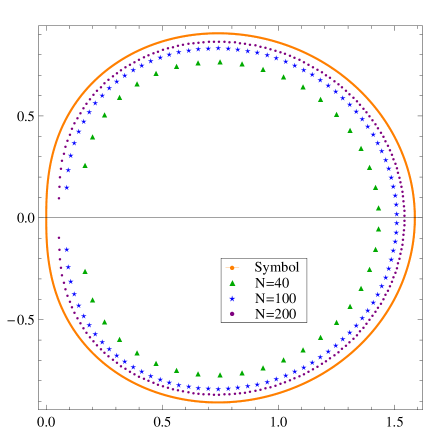
Figure 1: Eigenvalue Distribution. The image of the symbol together with the eigenvalues in the complex plane for $\alpha=1/3$, $\beta=-1/2$; the orange curve being the image of the symbol; the green triangles, blue stars and purple dots being the eigenvalues for $N=40$, $100$ and $200$ respectively.

To set the analysis of the eigenfunctions in a proper context we first show in Figure 1 a depiction of the eigenvalues for different $N$ and fixed $\alpha$ and $\beta$. The solid curve is theoretical. It shows the image of the symbol, $a(z)$, as $z$ traverses the unit circle. The dots are the eigenvalues calculated using Mathematica. According to Widom’s theory [10, 11], for many kinds of symbols, as $N$ goes to infinity, the spectrum of eigenvalues should approach that image. Specifically, the eigenvalues are approximately the ones given by the $N=\infty$ case in which fourier transformation gives $\epsilon^{l,N}=a(\exp(-ip^{l}))$, where the momenta, $p^{l}$ are uniformly spaced in $(0,2\pi)$. In symbols,

$$\epsilon^{l,N}=a\left(e^{-2\pi il/(N-1)}\right)+O\left(\frac{\ln N}{N}\right)$$ (10)

This figure shows that, for the case plotted here, the eigenvalues follow Widom’s prescription. In fact Eq.(10) is true for all $\alpha$ and $\beta$ which obey $0<\alpha<|\beta|<1$, which is the study range for this paper.

2.5 Different regions for eigenvector

The next two plots, Figure 2 and Figure 3 show respectively the gross behavior of the magnitude and phase of these eigenvectors, one with $N=100$ and $l=24$. Both plots show that, for large $N$, the ratios $\psi_{j+1}/\psi_{j}$ are constant throughout a broad central region of $j$, extending perhaps to from small values of $j/(N-1)$ to $j/(N-1)\approx 0.7$. This behavior changes markedly within the first few values of $j$ and above $j/(N-1)\approx 0.7$. We call these two regions respectively the initial region and the final region.

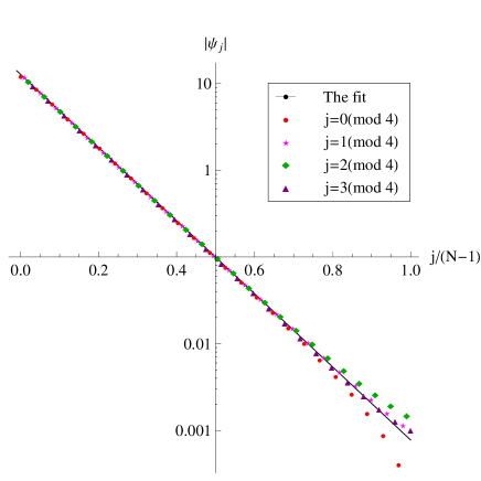
Figure 2: Magnitude of eigenvector. Here we plot $|\psi_{j}|$ against $j/(N-1)$ for $N=100$ and the eigenvalue with number $l=[(N-1)/4]$. If $l\sim pN/q$, with $p$ and $q$ being integers the phase goes through roughly $p$ revolutions as $j$ increases by $q$. For this particular value of $l$ there are four different branches to the eigenfunction and there is a repetition after every four steps of $j$. The four branches are indicated by different colors and shapes in this and the next figure. The solid line is an exponential fit to the data. The parameter values are $\alpha=1/3$ and $\beta=-1/2$.

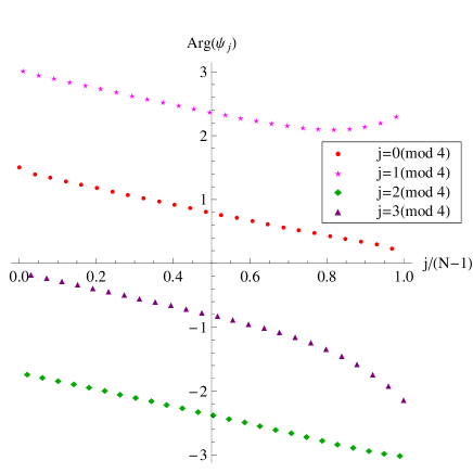
Figure 3: Phase of eigenvector. We plot the phase of the eigenvectors against $j/(N-1)$. The overall behavior is that successive points increase their phase by an amount close to $(2\pi)/4$. We again show the behavior as four branches, each with points separated by four steps of $j$, with the different branches being denoted by different colors and shapes. The branches are separated by a height difference of about $\pi/2$. The phase increases by an amount slightly smaller than $m\pi/2$ as $j$ advances by $m$ units. That is why the lines slope downward.

2.6 Central region

The first and most obvious characteristic of the central region is that over most of the region the eigenvector varies exponentially

$$\psi_{j}^{l,N}\approx\exp(ip^{l,N}j)$$ (11)

as indicated by the straight line behavior of exponent versus $j$ in Figure 2 and Figure 3. This behavior can most easily be understood as a consequence of the translational invariance of the matrix $T_{j,k}=T(j-k)$. The central region is far from the two ends $j=0$ and $j=N-1$. The eigenfunction in this region behaves as it would if we were able to push the two ends infinitely far away. We have picked $l=[(N-1)/4]$, so that this particular eigenfunction shows four different branches which differ in phase by roughly $\pi/2$.

2.7 Initial region

This branch-structure can also be discerned in the initial region (See Figure 4.) In this plot, each branch shows a few bumps for small values of $j$. The bumps decrease in size as $j$ increases and the branches approach one another in magnitude. (Their phases differ by about $(2\pi)/4$.) The behavior then settles down to the exponential decay seen in the central region. The behavior in the initial region does not appear to vary with $N$ for large values of $N$. Different values of $N$ show $\psi$ versus $j$ plots which have, for small values of $j$, exactly the same shape (See Figure 5.)

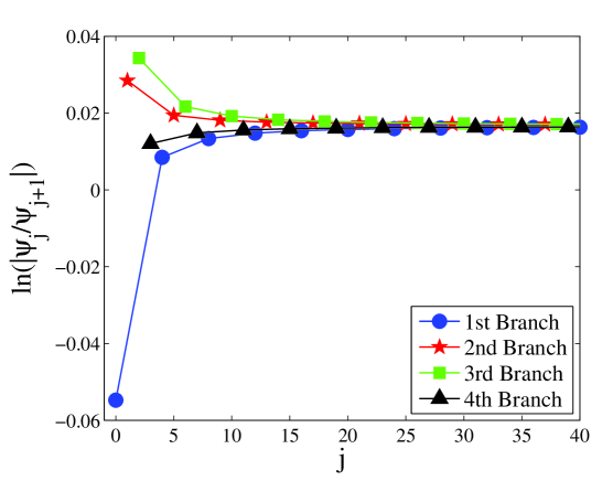
Figure 4: Magnitude of eigenvector in initial region. Here we plot four branches of the eigenvector labeled by $k=0,1,2,3$. Each branch has $j=k({\rm mod}{\rm~{}}4)$. For each branch, $\ln|\psi_{j}/\psi_{j+1}|$, is plotted against $j$ for the eigenvalue with number $l=[(N-1)/4]$, $N=801$, and parameter-values of $\alpha=1/3$, $\beta=-1/2$. The curves each show their different individual behavior for small $j$ and then become almost identical to one another for larger $j$.

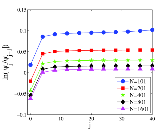
Figure 5: Magnitude of eigenvector in initial region for one branch. Here we plot $\ln|\psi_{j}/\psi_{j+1}|$, against $j=4k$ for $N=101,201,401,801$ and $1601$ for the eigenvalue with number $l=[(N-1)/4]$ and parameter-values of $\alpha=1/3$, $\beta=-1/2$. One can see that the shape of the curves does not change appreciably as $N$ varies. So the initial region contains eigenvectors with $N$-independent shapes.

2.8 Final region

Figure 6 and Figure 7 show eigenfunction for relatively large values of $j/(N-1)$. We note from the former figure that the four branches have different shapes in this region. However, Figure 7 shows that the shapes of the different branches settle down to an $N$-independent form as $N$ goes to infinity. However, the scaling in this region appears to be somewhat complex. We leave a further analysis of this region to a later publication.

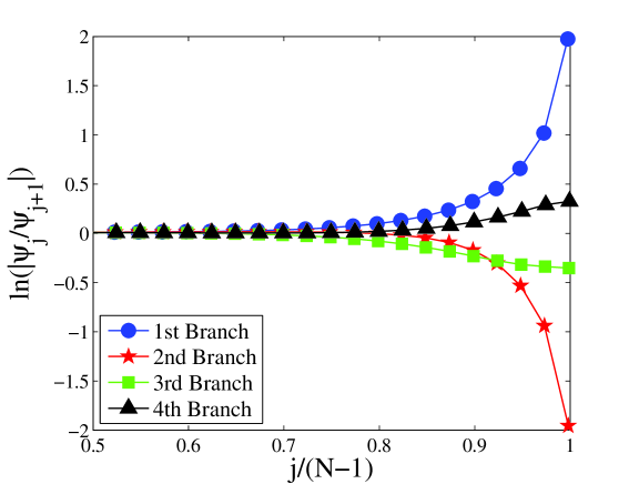
Figure 6: Magnitude of eigenvector in ending region. Here we plot $\ln|\psi_{j}/\psi_{j+1}|$, against $j$ for $N=1601$ and the eigenvalue with number $l=[(N-1)/4]$ and parameter-values of $\alpha=1/3$, $\beta=-1/2$. The four-branch structure is clearly indicated.

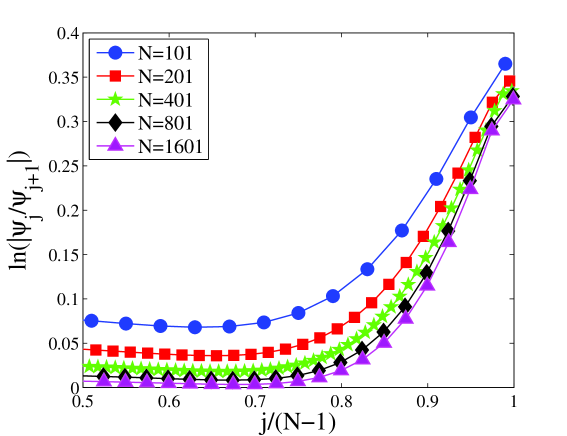
Figure 7: Magnitude of eigenfunction in ending region for one branch. Here we plot $\ln|\psi_{j}/\psi_{j+1}|$, against $j=4k$ for $N=101,201,401,801,1601$ and the eigenvalue with number $l=[(N-1)/4]$ and parameter-values of $\alpha=1/3$, $\beta=-1/2$. One can see that the shape of the curves does not change much as $N$ varies.

3 Quasi-particle results

In the 1950s, Landau [13, 14] worked out a theory of a low-temperature Fermi liquid, e.g. He³, which argued that the Fermi liquid was just like a non-interacting Fermi gas except that it had a different relation between energy and momentum. Here, we would like to make the same kind of argument.

3.1 “Energy”-momentum relation

We follow Landau in saying that the relevant “momentum”, $p$, appears in the phase of the eigenfunction as $\exp(ipj)$. In the idealized case, $N=\infty$, corresponding to Landau’s non-interacting case, the phase and eigenvalue obey $\epsilon=a(\exp(-ip))$. We carry this result over directly to finite values of $N$ as in Equation II of the Abstract. We write that equation in terms of $a^{-1}(\cdot)$, the function inverse to $a(\cdot)$, to define

$$p_{\epsilon}^{l}=i\ln a^{-1}(\epsilon^{l})$$ (12a)

The momentum variable defined from the wave function will be written as $$p_{\psi}$$. One possible definition is

$$p_{\psi}^{l}=-i[\ln\psi_{J}^{l}-\ln\psi_{j}^{l}]/(J-j)$$ (12b)

Here we must pick the branch of the logarithm in Eq.(12) so as to make $p_{\psi}$ approximately equal to $2\pi l/N$. We need to figure out whether, the two definitions give results that are substantially equal in the large $N$ limit, for example, whether it is true that

$$p_{\psi}^{l}=p_{\epsilon}^{l}+o(1/N)$$ (13)

Eq.(13) and the equations in the abstract are all checked using Tables 1 through 4. All four tables analyze the data for $\alpha=1/3$ and $\beta=-1/2$. The first two tables use data for the imaginary part of $p$, while the latter two refer to the real part of $p$. In each case, the $p_{\psi}$ in the table is obtained by using Eq.(12b) with $J=[0.5N]$ and $j=[0.2N]$. The first two lines in each table describe the $p$-values thus obtained. They are seen to be increasingly close for larger values of $N$. The next line gives the difference between these values multiplied by powers of $N$. No one of these lines increases substantially as $N$ increases. This result confirms Eq.(13), which states that the two methods of determining $p$ are consistent with one another in the limit of large $N$. In fact these results tend to indicate that the difference between these two estimates of $p$ is of order $1/N^{3}$ for the imaginary part and $1/N^{2}$ for the real part. Thus we have verified Equation II of the abstract.

Next we compare the $p$-values in the table with Equation I of the abstract. The next to last row of the table gives the value of $N$ times the first row. According to Equation I, that row should be fitted by $i(2\alpha+1)\ln N+C$, where $C$ is a complex constant. The final row gives the errors for each $N$ after the corresponding theoretical result is subtracted away. Each table thus involves one adjustable constant. The small values of the remainder in the last row indicate that Equation I of the abstract appears to be quite justified. The fit for Table 1 is shown in graphical form in Figure 8.

$N$	$2000$	$1000$	$400$	$200$	$100$	$40$
$\Im(p_{\psi})$	$0.00765381$	$0.0141435$	$0.0314841$	$0.0570298$	$0.101950$	$0.213238$
$\Im(p_{\epsilon})$	$0.00765381$	$0.0141435$	$0.0314842$	$0.0570311$	$0.101961$	$0.213463$
difference$\cdot 10^{6}$	$-0.00111$	$-0.00881$	$-0.146$	$-1.29$	$-11.7$	$-225$
difference$\cdot N^{3}$	$-8.85$	$-8.81$	$-9.36$	$-10.3$	$-11.7$	$-14.4$
$\Im(p_{\psi})\cdot N$	$15.308$	$14.146$	$12.594$	$11.406$	$10.195$	$8.530$
$\Im(p_{\psi})\cdot N-{\rm Fit}$	$0$	$-0.00886$	$-0.0316$	$-0.0640$	$-0.120$	$-0.258$

Table 1: Two estimates of the imaginary part of $p$ are shown to be substantially equal. They are then successfully fit to the theory. The value of $l$ for this table is $l=[(N-1)/2]$. The third line shows the difference of the two estimates and the fourth line shows that difference multiplied by $N^{3}$. The rough constancy of this line with increasing $N$ supports the correctness of Eq. (13). The next to last line shows the result of multiplying the imaginary part of $p_{\psi}$ in the top row by $N$. According to the theory this quantity should be $(2\alpha+1)\ln N+\Im(C)$. We get a good fit to these data by using $\Im(C)=2.639$. The last row in the table is the result of subtracting this fit from the result in the previous row. It represents the error in our analysis. Since the relative error is so small, we argue that Equation I of the abstract is corroborated.

These results of this comparison are shown in Table 1 for $p$ roughly equals to $\pi/2$. Table 2 shows the same analysis applied to an “irrational” value of $p$ chosen by taking $l=[(\sqrt{5}-1)(N-1)/2]$. Tables 3 and 4 give a similar comparison for the real part of $p$. In all cases Eq.(13) appears to be justified.

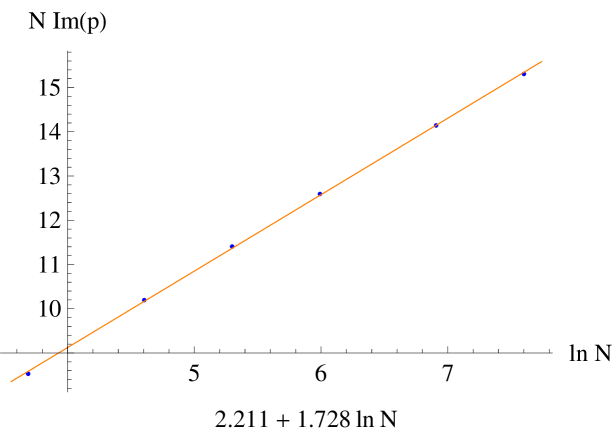
Figure 8: Imaginary part of $p$. This plot shows the data in the next to last row of Table 1 plotted along with a least squares fit. The theoretical slope is $1.667$ and the fitted one is $1.728.$

$N$	$2000$	$1000$	$400$	$200$	$100$	$40$
$\Im(p_{\psi})$	$0.00761559$	$0.0140678$	$0.0313017$	$0.0566988$	$0.101397$	$0.212772$
$\Im(p_{\epsilon})$	$0.00761559$	$0.0140678$	$0.0313018$	$0.0566981$	$0.10141$	$0.212644$
difference$\cdot 10^{6}$	$0.000137$	$0.00964$	$-0.0699$	$0.680$	$-13.4$	$128$
difference$\cdot N^{3}$	$1.10$	$9.64$	$-4.48$	$5.44$	$-13.4$	$8.17$
$\Im(p_{\psi})\cdot N$	$15.231$	$14.068$	$12.521$	$11.340$	$10.140$	$8.511$
$\Im(p_{\psi})\cdot N-{\rm Fit}$	$0$	$-0.00811$	$-0.0281$	$-0.0538$	$-0.0986$	$-0.200$

Table 2: The same as Table 1 except that the values of $l$ are given by $l=[(\sqrt{5}-1)(N-1)/2]$.

$N$	$2000$	$1000$	$400$	$200$	$100$	$40$
$\Re(q_{\psi})\cdot 10^{6}$	$3.80031$	$14.4177$	$84.7912$	$326.402$	$1265.36$	$7661.04$
$\Re(q_{\epsilon})\cdot 10^{6}$	$1.72814$	$6.91045$	$43.1505$	$172.352$	$687.673$	$4274.71$
difference$\cdot 10^{6}$	$2.07$	$7.51$	$41.6$	$154$	$578$	$3386$
difference$\cdot N^{2}$	$8.29$	$7.51$	$6.66$	$6.16$	$5.78$	$5.42$
$\Re(q_{\psi})\cdot N$	$0.00760$	$0.0144$	$0.0339$	$0.0653$	$0.127$	$0.306$
$\Re(q_{\psi})\cdot N-{\rm Fit}$	$0$	$0.00682$	$0.0263$	$0.0577$	$0.119$	$0.299$

Table 3: The same as Table 1, except that we examine here the real part of $q=p-2\pi l/(N-1)$. The fit on the last line sets $N$ times the real part equal to a constant, $0.00760$.

$N$	$2000$	$1000$	$400$	$200$	$100$	$40$
$\Re(q_{\psi})\cdot 10^{6}$	$-808.955$	$-1610.85$	$-4038.63$	$-7861.35$	$-14949$	$-26243.8$
$\Re(q_{\epsilon})\cdot 10^{6}$	$-810.805$	$-1617.64$	$-3997.34$	$-7726.56$	$-14391.3$	$-29846.7$
difference$\cdot 10^{6}$	$1.85$	$6.80$	$-41.3$	$-135$	$-558$	$3603$
difference$\cdot N^{2}$	$7.40$	$6.80$	$-6.61$	$-5.39$	$-5.58$	$5.76$
$\Re(q_{\psi})\cdot N$	$-1.618$	$-1.611$	$-1.615$	$-1.572$	$-1.495$	$-1.050$
$\Re(q_{\psi})\cdot N-{\rm Fit}$	$0$	$0.00707$	$0.00246$	$0.0456$	$0.123$	$0.568$

Table 4: The same as Table 2, except that we examine here the real part of $q=p-2\pi l/(N-1)$. The fit on the last line compares $N$ times the real part equal to a constant, $-1.618$. As one can see, this fit is quite accurate especially for the larger values of $N$.

3.2 Spacing of eigenvalues

The other part of quasi-particle theory that we wish to verify is that for successive $l$-values the $p^{l}$ should be spaced by $2\pi/N$. This will help ensure that the phase difference between $\psi_{0}^{l}$ and $\psi_{N-1}^{l}$ can remain independent of $l$. To check this we notice that the fits for the real part of $p$ in Tables 3 and 4 indicate that these two eigenvalues have their spacing correctly described by the two equations in the abstract. A brief examination shows that these spacings seem to continue to hold for all values of $l$ except the ones which have $l/(N-1)\ll 1$ or $1-l/(N-1)\ll 1$. Near these end-points different spacings are observed. In this paper, we do not pursue this point any further.

4 Wiener-Hopf method

4.1 The singly infinite eigenvalue problem

To get a good approximation for the Toeplitz matrix’s eigenvector, one might start by looking at the limiting case in which $N$ is infinity. The case in which the integer index, $j$, is extended from $-\infty$ to $\infty$ is simply solved by Fourier transformation as in Eq.(5) and Eq.(6). But the singly infinite case, described as the Toeplitz operator problem, in which $j$ extends from, say, $0$ to $\infty$ is much harder. The approach from singly infinite-$N$ to the case of $N$ large but finite is tricky and non-uniform. (We give an example of the non-uniformity below.) Nonetheless the singly infinite matrix provides a good entry into the finite-$N$ system.

We want to solve the Toeplitz operator eigenvalue-problem

$$\sum_{j=0}^{\infty}T_{kj}\psi_{j}=\epsilon\psi_{k},{\rm~{}for~{}all~{}}k\geq 0$$ (14a)

and the transpose problem

$$\sum_{j=0}^{\infty}\tilde{\psi}_{j}T_{jk}=\epsilon\tilde{\psi}_{k},{\rm~{}for~{}all~{}}k\geq 0$$ (14b)

where $T$ is a Toeplitz operator, i.e. $T_{jk}=T(j-k)$.

There is a well-developed theory, called the Wiener-Hopf method, for solving equations involving this kind of operator [15]. See for example [16] and Chapter IX of McCoy and Wu [5]. See also [17, 18] for applications close to the problem studied here. Following McCoy and Wu, we define a class of vectors with indices which run from $-\infty$ to $\infty$. The components of these special vectors are required to vanish for negative values of their index. The vectors of this type are indicated by the superscripts “$+$”. For example the “$+$” vector corresponding to an eigenfunction of the Toeplitz operator is written as

$$\psi_{j}^{+}=\left\{\begin{array}[]{cc}\psi_{j},&j\geq 0\\ 0,&j<0\end{array}\right.$$

then we can write the eigenvalue equation as

$$\sum_{k=-\infty}^{\infty}K_{jk}\psi_{k}^{+}=0{\rm~{}~{}for~{}all}~{}j\geq 0~{}~{}~{}~{}{\rm where}~{}~{}K_{jk}=T_{jk}-\epsilon\delta_{jk}$$

We would like to define an equation for the eigenfunction which covers the entire range, $(-\infty,\infty)$, for the variable $j$. To do that we define another kind of vector, one indicated by a superscript “$-$”. One example of such a vector is

$$\psi_{j}^{-}=\sum_{k=-\infty}^{\infty}K_{jk}\psi_{k}^{+},{\rm~{}for~{}all~{}integer~{}}j$$ (15)

In general, the vectors in this category vanish for $j>0$. However this particular vector also vanishes for index equal to zero. This extra condition will play an important role in our solution.

The result of this subsection is an eigenvalue equation which reads

$$\sum_{k=-\infty}^{\infty}K_{jk}\psi_{k}^{+}=\psi_{j}^{-}\makebox{~{}~{}for all integer~{}~{}}j$$ (16)

This equation has the same content as Eq.(14a).

4.2 Fourier transforms

Eq.(16) may be solved by Fourier transformation. Define

$$a(z) = \sum_{j=-\infty}^{\infty}T(j)z^{j}$$ (17)

$$\psi^{+}(z) = \sum_{j=-\infty}^{\infty}\psi_{j}^{+}z^{j}=\sum_{j=0}^{\infty}\psi_{j}^{+}z^{j}$$ (18)

$$\psi^{-}(z) = \sum_{j=-\infty}^{\infty}\psi_{j}^{-}z^{j}=\sum_{j=-\infty}^{-1}\psi_{j}^{-}z^{n}$$ (19)

Multiply Eq.(16) by $z^{j}$ and sum over all $j$, to give

$$\sum_{j=-\infty}^{\infty}\sum_{k=-\infty}^{\infty}(T_{jk}-\epsilon\delta_{jk})z^{j-k}\psi_{k}^{+}z^{k}=\sum_{j=-\infty}^{\infty}\psi_{j}^{-}z^{j}$$

which then gives an eigenvalue equation expressed in Fourier language:

$$K(z)\psi^{+}(z)=\left(a(z)-\epsilon\right)\psi^{+}(z)=\psi^{-}(z)$$ (20)

At this point, the eigenvalue equation has been reduced to an algebraic equation, one that may apparently be solved by algebraic manipulations. However, Eq.(20) has two unknowns, $\psi^{+}(z)$ and $\psi^{-}(z)$ so that additional knowledge is needed to obtain a solution for $\psi^{+}(z)$. That knowledge is based upon the analytic properties of the various functions.

4.3 Factorization

To find $\psi^{+}(z)$, we must factorize $K(z)=a(z)-\epsilon$ into a product of functions of the form

$$K(z)=z^{\nu}\frac{K^{+}(z)}{K^{-}(z)}$$ (21)

where $\nu$ is an integer determined by the form of $K(\cdot)$. It is called the winding number since it represents the total number of times the function wraps around zero when $z$ is rotated once around zero in the positive sense. The winding number obeys

$$\nu=\frac{1}{2\pi i}\intop_{0}^{2\pi}d\ln K(e^{ip})=\frac{1}{2\pi i}\left[\ln K(e^{2\pi i})-\ln K(e^{0i})\right]$$ (22)

This factorization is important since it will enable us to immediately construct a non-trivial solution to the Toeplitz operator equation in the one case, $\nu=-1$, in which this solution exists [16]. (See McCoy and Wu [5] page 208-215. The condition, $\nu=-1$, demands that the $j=0$ component of $\psi_{j}^{-}$ must be zero, as is required for our solution.)

A factorization like this can be derived simply when the function, $K(z)$, has no singularities or zeros on the unit circle and has none at zero or infinity. However, all these conditions fail in the Fisher-Hartwig case. But, McCoy and Wu [5] argue that the factorization also works with the definition, Eq.(22), of the winding number in the case in which $K(z)$ is only continuous, not analytic, on the unit circle and has appropriate analyticity properties in an analytic continuation away from that circle. Their analysis then covers the Fisher-Hartwig case in the range interesting to us: $0<\alpha<|\beta|<1$. If one applies this integral formula of Eq.(22) to find the winding number for $K$ one sees that

$$\nu=-1\mbox{~{}~{} for~{}~{}}-1<\beta<0,$$ (23a)

so this is the case in which the Toeplitz operator gives a non-trivial solution for the eigenvector. Conversely

$$\nu=1\mbox{~{}~{} for~{}~{}}0<\beta<1$$ (23b)

so there are only trivial eigenvector solutions in this situation.

McCoy and Wu also give us formulas for finding the functions $K^{\pm}(z)$. One starts from the contour integration

$$G^{\pm}(z)=\frac{1}{2\pi i}\ointctrclockwise_{S_{1}}dz^{\prime}\frac{\ln(z^{\prime-\nu}K(z^{\prime}))}{z^{\prime}-z}$$ (24)

Here the upper (and lower) signs respectively refer to the cases in which $z$ is inside (and outside) the unit circle. Then

$$K^{\pm}(z)=\exp[G^{\pm}(z)]$$ (25)

With these definitions, the eigenvalue equation has the form

$$\psi^{+}(z)K^{+}(z)=z^{-\nu}\psi^{-}(z)K^{-}(z)$$ (26)

The left hand side contains only non-negative powers of $z$. To say when we can have eigenvalues, we must look at the right hand side and see whether it can match the left. The three factors on the right hand side contains powers which are at a maximum $-\nu-1+0$, obtained from reading the three factors from left to right.

4.4 $\nu=-1$

The sole possibility of obtaining a solution to Eq.(26) comes from picking $\nu=-1$. Then the right hand side can match the left by simply having each side be a constant independent of $z$. Thus one finds

$$\psi^{+}(z)K^{+}(z)=z\psi^{-}(z)K^{-}(z)=C$$ (27)

where $C$ is a non-zero constant which will set the phase and magnitude of the wave function.

In this case, we have as our solution

$$\psi^{+}(z)=\frac{C}{K^{+}(z)}{\rm~{}~{}for~{}~{}}|z|<1$$ (28)

We have now obtained a solution in terms of quadratures.

Note that in general we expect that the $\nu$-value will remain constant as the eigenvalue varies over some open set. Thus one has a region in the complex plane in which the Toeplitz operator has eigenvalues. This result is in contrast to the outcome for the Toeplitz matrix which usually has $N$ isolated eigenvalues.

Example: A simple pole

We choose a very simple example to illustrate what we have said. Take $a$ to be of the Fisher-Hartwig type with $\alpha=0$ and $\beta=-1$: $a(z)=z^{-1}$ (See Eq.(3), where for convenience we have dropped the overall minus sign). The matrix, $T_{jk}$, is

$$T^{\infty}=\left[\begin{array}[]{ccccc}0&1&0&0&\cdots\\ 0&0&1&0&\cdots\\ 0&0&0&1&\cdots\\ 0&0&0&0&\cdots\\ \vdots&\vdots&\vdots&\vdots&\ddots\end{array}\right]$$ (29)

The equation $\phi=T\psi$ is equivalent to

$$\phi_{j}=\psi_{j+1}~{}~{}\makebox{for}~{}~{}j\geq 0.$$

Thus the operator $T=z^{-1}$ when it is acting to the right transfers information from large $j$ to smaller $j$. It is reasonable to assume that all operators with $\nu=-1$ similarly transfer information towards smaller $j$, and thereby they can effectively produce a boundary condition of a vector being zero as $j$ goes to infinity.

Take the eigenvalue to be $\epsilon$, with magnitude less than unity, so that it sits within the unit circle. Then

$$K(z)=z^{-1}-\epsilon=K^{+}/(zK^{-})$$

The factorization then gives

$$K^{+}(z)=1-\epsilon z\mbox{~{}~{}and~{}~{}}K^{-}(z)=1.$$

As required $K^{+}$ has its zero outside the unit circle. One therefore finds that the eigenfunction has a fourier transform

$$\psi^{+}(z)=\frac{C}{1-\epsilon z}=C\left(1+\epsilon z+(\epsilon z)^{2}+\cdots\right),$$

which in turn implies an exponentially decaying eigenfunction

$$\psi_{j}=C(\epsilon)^{j}\makebox{~{}~{}for~{}~{}}j=0,1,2,\cdots$$ (30)

Thus the entire unit circle is filled with eigenvalues while $\psi^{+}(z)$ has a single pole, and the eigenfunctions $\psi_{j}$ are geometrical series.

This situation is of the Fisher-Hartwig type with $\alpha=0$ and $\beta=-1$.

However, the finite Fisher-Hartwig matrix with this symbol has a very different behavior. This matrix, $T^{(N)}$ has $N$ unit entries just above the diagonal, with all the rest of the entries being zero. (Here the notation $T^{(N)}$ describes an $N$ order Toeplitz matrix and not the $N$th power of anything.) Thus it looks just like the infinite matrix of Eq.(29) except that it is truncated after $N$ rows and $N$ columns, i.e.

$$T^{(N)}=\left[\begin{array}[]{ccccc}0&1&0&0&\cdots\\ 0&0&1&0&\cdots\\ 0&0&0&1&\cdots\\ 0&0&0&0&\cdots\\ \vdots&\vdots&\vdots&\vdots&\ddots\end{array}\right]_{N\times N}$$ (31)

The eigenvalue equations read

$$\psi_{N-1}=0$$ (32a)

and

$$\psi_{N-1-j}=(1/\epsilon)\psi_{N-j}\makebox{~{}~{}for~{}~{}}j=1,2...N-1$$ (32b)

These equations are solved successively. They do not make sense for $\epsilon=0$. For all other values of $\epsilon$, the eigenvector has all of its elements being zero. As a result, all eigenfunctions are trivial.

Thus, the eigenfunction behavior of this particular order-$N$ Fisher-Hartwig matrix matches that of the corresponding operator only in the special case in which we set $C=0$ in the operator eigenvector.

5 Calculation of eigenfunctions

The work of previous authors on eigenvalues has given us useful but limited information. We have an asymptotic expansion which gives the line on which the eigenvalues fall and their probability density on that line. Their exact placement on that line has never been explicitly calculated. Nor have the eigenfunctions associated with these eigenvalues. Here, we set out to fill in some of these omissions, using both asymptotic calculations and numerical work. We shall especially make use of the Wiener-Hopf solutions outlined in the previous chapter to discuss the properties of the behavior arising from the Fisher-Hartwig generating function.

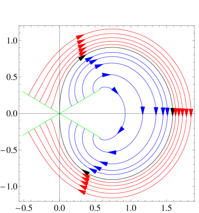
Figure 9: Maps of the symbol on the $w$-plane. The black curve is the image of the symbol $w=a_{\alpha,\beta}(z)$ for $\alpha=1/3$ and $\beta=-1/2$ with $z$ going around the unit circle in the counterclockwise direction. The symbol has a singularity at $z=1$ (mapped to $w=0$) as we can see from the other curves in this figure. The curves counting from the outmost are the images of this symbol for circles $|z|=0.75$, $|z|=0.8$, $|z|=0.85$, $|z|=0.9$, $|z|=0.95$, $|z|=1$, $|z|=1.1$, $|z|=1.2$, $|z|=1.4$, $|z|=2$ and $|z|=4$ respectively (red curves for $|z|<1$, blue curves for $|z|>1$ and the black curve for the unit circle). The green lines consist of the endpoints of the curves.

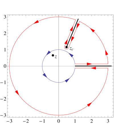
Figure 10: The singularities in the contour integral of in the $z^{\prime}$-plane for the integration in Eq.(34). The original contour, on the unit circle, is shown in blue. This path can then be deformed into the one shown in red, encircling singularities outside the unit circle. The black lines are encircled branch lines, including one starting at $z_{c}$, where $a(z^{\prime})=\epsilon$, and another along the positive real axis. The path on the big red circle can be taken to infinity where it does not contribute. The dot is the singularity at $z^{\prime}=z_{c}$. There is an additional pole singularity at $z^{\prime}=z$, which does not contribute because $z$ is inside the unit circle.

For $0<\alpha<-\beta<1$, all the eigenvalues lie within the closed curve formed as the image of the unit circle mapped by the symbol. Since the image winds around in the clockwise direction, the winding number of $(a_{\alpha,\beta}-\epsilon)$ is $-1$ for any eigenvalue, $\epsilon$. Therefore, we can use the quadrature of the previous chapter,

$$\psi^{+}(z)=Ce^{-G^{+}(z)}$$ (33)

where

$$G^{+}(z)=\frac{1}{2\pi i}\ointctrclockwise_{S_{1}}dz^{\prime}\frac{\ln[z^{\prime}(a_{\alpha,\beta}(z^{\prime})-\epsilon)]}{z^{\prime}-z}$$ (34)

This result is then a solution by quadratures of the Toeplitz operator problem involving the Fisher-Hartwig symbol. We may assume that this solution is accurate for small positive values of $x=j/(N-1)$ and becomes less accurate as $x$ approaches one from below.

5.1 Evaluation of the integrals

Eq.(33) and Eq.(34) together give the result for the Fisher-Hartwig symbol for the case $0<\alpha<-\beta<1$. Figure 1 shows the image of the unit circle formed by the symbol together with the eigenvalues of the corresponding Toeplitz matrices for the case $\alpha=1/3$, $\beta=-1/2$. We see that the eigenvalues are all distributed inside the image of the symbol. They approach that image as the size of the Toeplitz matrix goes to infinity. Further discussion of the asymptotic behavior of the eigenvalues has been given in [12].

To perform the contour integration in Eq.(34), we need to rewrite our symbol in terms of an analytic function, which is

$$a_{\alpha,\beta}(z)=(z-1)^{2\alpha}z^{\beta-\alpha}e^{-i(\beta+\alpha)\pi}$$ (35)

We shall choose this function, which has branch points at zero, one, and infinity, to have a branch cut along the positive real axis (See Figure 10). The logarithm in Eq.(34) has an additional singularity at the point, outside the unit circle, where $a(z^{\prime})$ equals the eigenvalue. We call this point $z_{c}$. It obeys

$$a(z_{c})=\epsilon$$ (36)

We can then have another branch line extending from $z_{c}$ to $\infty$. As $N$ goes to infinity, $\epsilon$ approaches the image of the unit circle and $z_{c}$ approaches the unit circle. These points will play important roles in what follows. Since $a(z^{\prime})$ goes exponentially to zero at infinity the contour in Eq.(34) can be deformed as shown in Figure 10. The big circular path can then be taken to $\infty$. The result is that our integral becomes, aside from an additive constant,

$$G^{+}(z)=L(z)+S(z)$$ (37a)

Here $$L(z)$$ stands for a logarithmic term, which is

$$L(z)=\ln(z-z_{c})$$ (37b)

while $$S(z) z=1$$ stands for a term which has a weak singularity at ,

$$S(z)=\frac{1}{2\pi i}\intop_{1}^{\infty}\frac{dt}{t-z}\ln\left[\frac{(t-1)^{2\alpha}t^{\beta-\alpha}e^{-i(\beta+\alpha)\pi}-\epsilon}{(t-1)^{2\alpha}t^{\beta-\alpha}e^{i(\beta+\alpha)\pi}-\epsilon}\right]$$ (37c)

Here, $z_{c}$ is the position of the zero in $K(z)=a(z)-\epsilon$ in the $z$-plane. According to Widom’s ideas, this zero approaches the unit circle as $N$ goes to infinity, but remains outside of that circle. This approach makes for a near-singularity in $\psi^{+}(z)$ on the circle. For $z$ inside the circle, this near-singularity looks like a singularity just outside the point $z=\exp(-2\pi il/(N-1))$. In contrast the real singularity in $\psi^{+}(z)$ is produced by the branch line which passes through $z=1$. The singularity and the near-singularity are well separated except for situations in which $l$ is relatively close to $l=0$ or $l=N-1$. We have not explored these exceptional limiting cases.

5.2 Accuracy of Wiener-Hopf solution

The solution we have generated is exact in the limiting case in which $j$ is fixed and $N$ goes to infinity. Thus, we might expect that the solution is accurate for large $N$ and fixed $j/(N-1)$. To see how accurate it is, we plot in Figure 11 the absolute value of the difference between the Wiener-Hopf quadrature and the exact solution for $N=1000$. The absolute value of the error never gets larger than a few times $10^{-7}$. It decreases slowly as $j/(N-1)$ increases. The relative error, plotted in Figure 12, grows with $j/(N-1)$, starting from order $10^{-7}$ and increasing to order one at $j/(N-1)\approx 1$. Therefore, we may say that the Wiener-Hopf solution reproduces the main features of the exact eigenfunction except very close to the maximum values of $j/(N-1)$.

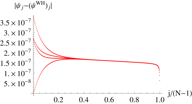
Figure 11: Absolute comparison of Wiener-Hopf solution with exact eigenfunction. The magnitude of the difference between the Wiener-Hopf solution and the exact eigenfunction is plotted against $j/(N-1)$ for $N=1000$, $l=[(N-1)/4]$, $\alpha=1/3$ and $\beta=-1/2$.

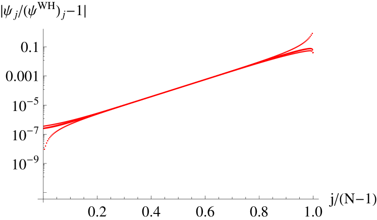
Figure 12: Relative comparison of Wiener-Hopf solution with exact eigenfunction. The relative magnitude, $\left|\psi/\psi^{WH}-1\right|$ of the difference between the Wiener-Hopf solution and the exact eigenfunction is plotted against $j/(N-1)$ for $N=1000$, $l=[(N-1)/4]$, $\alpha=1/3$ and $\beta=-1/2$.

5.3 Examination of solution

Even a superficial examination of Eq.(37) shows that its behavior fits the known properties of the eigenfunction. One term in the wave function is

$$\psi_{L}(z)=\exp\left(-L(z)\right)=-\frac{1}{z_{c}(1-z/z_{c})}=-\frac{1}{z_{c}}\sum_{j=0}^{\infty}\left(z/z_{c}\right)^{j}$$ (38)

This part of $\psi(z)$ thus produces a $\psi_{j}$ which is

$$(\psi_{L})_{j}=-(1/z_{c})^{j+1}$$ (39)

This structure is exactly the decaying exponential so evident in the central region of $j$.

The other parts of $\psi(z)$ come from $\psi_{S}(z)=\exp\left(-S(z)\right)$. This exponential is independent of $N$ except for the very weak $N$-dependence produced by a very small additive term of the form $\gamma(\ln N)/N$ in the eigenvalue, $\epsilon$. This effect of the $N$-dependence in this term is quite negligible.

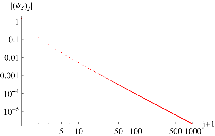
Figure 13: Expansion of $\psi_{S}$. The magnitude of the terms in the expansion of $\psi_{S}(z)$ in powers of $z$. These terms reflect corrections to the eigenfunction beyond the leading exponential behavior. The notable features are a long tail proportional to $(j+1)^{-2\alpha-1}$ and a few decreasing order-one bumps for small $j$.

Figure 13 plots the magnitude of the terms in the power series expansion of $\psi_{S}(z)$ in $z$. Using the same notation as used for $\psi_{L}(z)$, these terms are called $(\psi_{S})_{j}$. The first few terms are of order unity and produce the small-$j$ bumps evident in Figure 4. The bumps slowly die away for higher $j$.

For higher $j$ the behavior of $(\psi_{S})_{j}$ is dominated by a power law behavior, which shows up as a straight line in Figure 13. Even though these terms fall off, this contribution remains significant. This behavior is shown in Eq.(40). It results from a singularity as $z$ goes to unity evidenced in Eq.(37c), which shows a behavior for small $z-1$ of the form

$$\ln\psi_{S}(z)\sim-\frac{\sin\pi(\alpha+\beta)}{\pi~{}\epsilon}\int_{0}^{L}~{}ds~{}\frac{s^{2\alpha}}{1+s-z}$$

$L$ is a large number which serves as a cutoff at large values of $s$. This expression can be expanded in a power series in $z$, with coefficients of high order terms in the form

$$\left[\ln\psi_{S}(z)\right]_{j}\sim-\frac{\sin\pi(\alpha+\beta)}{\pi~{}\epsilon}\int_{0}^{L}~{}ds~{}\frac{s^{2\alpha}}{(1+s)^{j+1}}$$

For large $j$ the integral contributes for small values of $s$, of order $1/j$ so that we can replace $(1+s)^{j+1}$ by $e^{s(j+1)}$. We thus get the leading singularity in $\ln\psi_{S}(z)$ to be given by

$$[\ln\psi_{S}(z)]_{j}\sim-\frac{\Gamma(2\alpha+1)\sin\pi(\alpha+\beta)}{\pi~{}\epsilon~{}(j+1)^{2\alpha+1}}$$ (40)

Since this singularity in $\ln\psi_{S}(z)$ indicates a zero added onto a leading term which is a constant, the very same form of singularity appears in $\psi_{S}(z)$, which therefore has a high order expansion

$$[\psi_{S}(z)]_{j}\sim-\frac{\Gamma(2\alpha+1)\sin\pi(\alpha+\beta)}{\pi~{}\epsilon~{}(j+1)^{2\alpha+1}}$$ (41)

for large values of $j$.

5.4 Mixed terms

5.4.1 Sums

So far we have argued that the solution for $\psi_{j}$ should contain terms of the exponential form shown in Eq.(39) as well as the algebraic form in Eq.(41). In addition there is a set of bumps which appear only for small $j$. For larger $j$, then, we might expect an eigenfunction which looks like

$$\psi_{j}\sim A(z_{c})^{-j-1}+B(j+1)^{-(2\alpha+1)}$$ (42)

where $A$ and $B$ are both constants. Since both terms are generated near $j=0$, we expect both $A$ and $B$ to be of order unity. Note that both terms fall off for higher $j$. If, as we expect, $\Re\left(\ln 1/z_{c}\right)$ is small, then the exponential decay will be slow for small $j$, while the decay of the algebraic term will be rapid. However, for sufficiently large $j$ the two terms return to being of the same order. We assume this equality is achieved when $j=O(N)$ so that we might have a boundary condition in which the two terms effectively interfere to produce a very small result near and beyond the border at $j=N-1$:

$$(z_{c})^{-N}\sim N^{-(2\alpha+1)}$$

Since $z_{c}=\exp(-ip)$, we can calculate the imaginary part of $p$ as

$$\Im\left(p\right)=\Re\left(\ln z_{c}\right)=(2\alpha+1)\frac{\ln N}{N}+O(1/N)$$ (43)

The $O(1/N)$ term arises from the ratio of $A/B$ in Eq.(42). This change in $p$ enables one to calculate the shift in the eigenvalue in the form

$$\frac{\delta\epsilon}{\epsilon}=\frac{\partial\ln\epsilon}{\partial p}\Im\left(p\right)$$

so that the change in the eigenvalue is given by

$$\frac{\delta\epsilon}{\epsilon}=\left(\beta+i\alpha\cot\frac{p}{2}\right)(2\alpha+1)\frac{\ln N}{N}$$ (44)

This is, to our knowledge, the first calculation of the eigenvalue shift for $\alpha$ not equal to zero.

5.4.2 Products

The actual form of the Wiener-Hopf eigenfunction is not a sum of the form shown in Eq.(42) but instead a product in which

$$\psi(z)\sim(z-z_{c})^{-1}\psi_{S}(z)$$ (45)

which can be Fourier transformed to give

$$\psi_{j}\sim\frac{\Gamma(2\alpha+1)\sin\pi(\alpha+\beta)}{\pi~{}\epsilon~{}z_{c}}\sum_{k=0}^{j}z_{c}^{-j+k}\frac{1}{(k+1)^{2\alpha+1}}$$ (46)

We introduce an integral representation for the last factor to give

$$\psi_{j}\sim\frac{\sin\pi(\alpha+\beta)}{\pi~{}\epsilon~{}z_{c}}\int_{0}^{\infty}~{}d\mu~{}\mu^{2\alpha}\sum_{k=0}^{j}e^{-(k+1)\mu}z_{c}^{-j+k}$$

The geometric series can be summed to find

$$\psi_{j}\sim\frac{\sin\pi(\alpha+\beta)}{\pi~{}\epsilon}\left[\int_{0}^{\infty}~{}d\mu~{}e^{-\mu}\mu^{2\alpha}\frac{z_{c}^{-j-1}-e^{-\mu(j+1)}}{1-z_{c}e^{-\mu}}\right]$$

This elegant result enables us to write $\psi_{j}$ as a sum of two terms:

$$\psi_{j}\sim Az_{c}^{-j-1}+B(j+1)^{-(2\alpha+1)}$$ (47a)

where the term multiplied by $$A$$ dominates in the central region and both terms are of the same order in the ending region. Here the value of the coefficients are

$$A\sim\frac{\sin\pi(\alpha+\beta)}{\pi~{}\epsilon}\int_{0}^{\infty}~{}d\mu~{}e^{-\mu}\mu^{2\alpha}\frac{1}{1-z_{c}e^{-\mu}}$$ (47b)

and

$$B\sim-\frac{\sin\pi(\alpha+\beta)}{\pi~{}\epsilon}\int_{0}^{\infty}~{}d\mu~{}e^{-\mu}\mu^{2\alpha}\frac{1}{1-z_{c}e^{-\mu/(j+1)}}$$ (47c)

To construct this form for $B$ we have made the change of variables $\mu\rightarrow\mu/(j+1).$ Note that this expression gives an eigenfunction of precisely the same form as we have analyzed in Eq.(42) in the previous subsection. Therefore the previous analysis will hold, if we assume that the coefficients $A$ and $B$ are constants. The only problem is that the integrals for $A$ and $B$ have singularities if $z_{c}$ is close to unity. For large $N$ this value of $z_{c}$ will only occur if $l/(N-1)$ or $\left(1-l/(N-1)\right)$ is very small. If we are not in those special regions of $l$, then $A$ and $B$ can be considered to be constants of order unity so that our previous estimate of the eigenvalue given by Eq.(44) will hold.

6 More to investigate

This paper is only a partial investigation of the problem at hand. It focuses on obtaining a good solution for smaller values of $j/(N-1)$ and does not look in detail at values of $j/(N-1)$ very close to one. In particular, the form of large-$j$ scaling is not considered. One might expect that some sort of Wiener-Hopf solution might be obtained on the large-$j$ side and that values of $p^{l}$ and $\epsilon^{l}$ might be calculable through order $1/N$.

No calculations are extended to the case $\alpha=0$, nor to the case in which $|\beta|<\alpha$.

We have shed no light on the source of the Fisher-Hartwig $\alpha^{2}-\beta^{2}$ in the determinant of $T$ nor have we explained what happens when $l/(N-1)$ is close to zero or one.

Nonetheless this paper does contain a large number of new results: we see excellent eigenfunctions for smaller $j$, and corrections in $p^{l}$ and $\epsilon^{l}$ to order $(\ln N)/N$. More importantly we have shed some light on how the logarithms arise to permit the interference between an exponential and an algebraic term in the eigenfunction. In all of this, we have made a novel use of “quasi-particle” theory a la Landau.

References

- [1] Böttcher A and Silbermann B, Introduction to Large Truncated Toeplitz Matrices, 1999 Springer
- [2] Trefethen L and Embree M, Spectra and Pseudospectra, 2005 Princeton University Press
- [3] Forrester P and Frankel N E, Applications and Generalizations of Fisher-Hartwig Asymptotics, 2004 J. Math. Phys. 45 2003-2028
- [4] Montroll E W, Potts R B and Ward J C, Correlations and spontaneous magnetization of the two-dimensional Ising model, 1963 J. Math. Phys. 4 308-322
- [5] McCoy B M and Wu T T, The Two-Dimensional Ising Model, 1973 Harvard University Press
- [6] Kadanoff L P, Spin-Spin Correlation in the Two-Dimensional Ising Model, 1966 Il Nuovo Cimento B 44 276-305
- [7] Szegö G, Ein grenzwertsatz über die Toeplitzschen Determinanten einer reellen positiven Funktion, 1915 Funktion. Math. Ann. 76 490-503
- [8] Fisher M E and Hartwig R E, Toeplitz determinants, some applications, theorems and conjectures, 1968 Adv. Chem. Phys. 15 333-353
- [9] Fisher M E and Hartwig R E, Asymptotic behavior of Toeplitz matrices and determinants, 1969 Arch. Rat. Mech. Anal. 32 190-225
- [10] Widom H, Toeplitz determinants with singular generating functions, 1973 Amer. J. Math. 95 333-383
- [11] Widom H, Eigenvalue distribution of nonselfadjoint Toeplitz matrices and the asymptotics of Toeplitz determinants in the case of nonvanishing index, 1990 Operator Theory: Adv. and Appl. 48 387-421
- [12] Lee S Y, Dai H and Bettelheim E, Asymptotic eigenvalue distribution of large Toeplitz matrices, 2007 arXiv: 0708.3124v1
- [13] See Wikipedia article on Fermi Liquid
- [14] Baym G and Pethick C, Landau Fermi-Liquid Theory: Concepts and Applications, 2008 Wiley-VCH
- [15] Wiener N and Hopf E, Über eine Klasse singuläer Integralgleichungen, 1931 Sitz. Berlin. Akad. Wiss. 696-706
- [16] Gokhov F D, Boundary Value Problems, 1966 Pergamon Press, Addison-Wesley Pub. Co.
- [17] Ohtaka K and Tanabe Y, Theory of the soft-x-ray edge problem in simple metals: historical survey and recent developments, 1990 Rev. Mod. Phys. 62 929-991
- [18] Nozieres P and De Dominicis C T, Singularities in the X-Ray Absorption and Emission of Metals. III. One-Body Theory Exact Solution, 1969 Phys. Rev. 178 1097-1107
- [19] Basor E and Morrison K E, The Fisher-Hartwig Conjecture and Toeplitz Eigenvalues, 1994 Linear Algebra Appl. 202 129-142