A Spherical Plasma Dynamo Experiment

Abstract

We propose a plasma experiment to be used to investigate fundamental properties of astrophysical dynamos. The highly conducting, fast-flowing plasma will allow experimenters to explore systems with magnetic Reynolds numbers an order of magnitude larger than those accessible with liquid-metal experiments. The plasma is confined using a ring-cusp strategy and subject to a toroidal differentially rotating outer boundary condition. As proof of principle, we present magnetohydrodynamic simulations of the proposed experiment. When a von Kármán-type boundary condition is specified, and the magnetic Reynolds number is large enough, dynamo action is observed. At different values of the magnetic Prandtl and Reynolds numbers the simulations demonstrate either laminar or turbulent dynamo action.

1 Introduction

One of the central problems of astrophysical fluid dynamics is the magnetohydrodynamic (MHD) dynamo, the process by which the motion of an electrically conducting fluid amplifies a small seed magnetic field until the field becomes dynamically important. Astrophysical dynamos can be categorized into two types: the large-scale dynamo, where the scale of the generated magnetic field is the same as or larger than the system generating it, such as in planets or stars, or the small-scale dynamo, where the scale of the magnetic field is much smaller than the system size, such as in warm interstellar medium (Kulsrud, 1999). Of particular physical importance in this context is the system’s magnetic Prandtl number, $Pm=\nu/\eta$, where $\nu$ is the kinematic viscosity of the fluid and $\eta$ its magnetic diffusivity, whose value indicates the scale of the velocity field at the resistive-diffusive cutoff. When $Pm\ll 1$ the magnetic-diffusion scale is in the hydrodynamic inertial range and the primary interactions are at that scale. If a dynamo occurs in this situation it is often large scale, though recent evidence indicates that a small-scale dynamo may also be possible (Iskakov et al., 2007; Schekochihin et al., 2007). Conversely, $Pm\gg 1$ gives a magnetic-diffusion scale below the viscous-diffusion cutoff, permitting the stretching and folding of the magnetic field at small scales and allowing the opportunity for a small-scale dynamo.

The small-scale dynamo has only been studied theoretically and through numerical simulations (see Haugen et al. (2004); Schekochihin et al. (2007) and references therein). The simulations tend to be done in periodic boxes with random non-helical forcing, in the absence of a mean flow, allowing the study of the dynamo under homogeneous and isotropic fluctuating conditions. Most simulations have been done in the range of $Pm\sim 1$, meaning with identical viscous and magnetic dissipation scales, though there have been notable exceptions where much higher values of $Pm$ (Schekochihin et al., 2004, 2002; Kinney et al., 2000) and values with $Pm<1$ (Iskakov et al., 2007; Schekochihin et al., 2007) have been used. Despite the large body of numerical and theoretical work on such dynamos, small-scale dynamos have never been experimentally studied due to the dearth of fluids for which $Pm\gg 1$ or $Pm\sim 1$. The only fluids which satisfy these criteria are plasmas, and plasma dynamo experiments, to study large or small-scale dynamos, have not thus far been constructed.

In contrast, several groups have recently been successful in achieving large-scale dynamo action in experiments using liquid sodium, a fluid for which $Pm\ll 1$ (Gailitis et al., 2000; Stieglitz & Müller, 2001; Monchaux et al., 2007). In such experiments the magnetic Reynolds number, $Rm=v_{0}a/\eta$, where $v_{0}$ is a characteristic speed, and $a$ a length scale, characterizes the ratio of magnetic field advection to diffusion. For idealized laminar velocity fields the critical value of $Rm$ for magnetic self-excitation, $Rm_{\rm crit}$, is predicted to be around 100 (Forest et al., 2002; Ravelet et al., 2005). To achieve this using liquid sodium in an experiment of radius $a=0.5$ m requires a mechanical input power of $P_{\rm mech}\sim 100$ kW. These flows are very turbulent, however, and turbulent flows have the unfavorable scaling $Rm\propto(P_{\rm mech}a)^{1/3}$. It would be interesting to study dynamo physics at a higher order of magnitude, $Rm=1000$ for example, but to achieve such a value of $Rm$ in a sodium experiment of similar size would require a mechanical input power of 100 MW! This is a serious limitation to addressing higher-$Rm$ dynamo regimes using liquid sodium.

A different class of fluids which could be used to study dynamo physics is plasma. To match the conductivity of sodium a singly ionized plasma requires an electron temperature of 630 eV, a plasma temperature only found in fusion experiments. However, plasma flows can be efficiently driven to much higher speeds than liquid metals. Thus for a plasma experiment of similar size ($a=1$ m) to achieve a value of $Rm=1000$ would simultaneously require an electron temperature of only $T_{\rm e}$ = 10 eV and a velocity $v_{0}$ = 20 km s^-1. These are modest values which can easily be achieved in many plasma confinement configurations. Plasma experimenters also have the novel ability to change the viscosity of their plasmas by several orders of magnitude. Such flexibility could allow the exploration of laminar and turbulent dynamos in a wide range of $Pm$, from $Pm\ll 1$ to $Pm\gg 1$. Such variability would be a striking improvement over liquid-metal experiments.

However, plasmas suffer from an important disadvantage when compared to liquid metals: they can be difficult to control and confine without the presence of a magnetic field. This is a problem for the study of dynamos, of course, because the presence of a dynamically significant magnetic field changes the fundamental behavior of the problem under study. Those challenges common to most plasma experiments–the need for thermal confinement to keep the plasma away from container walls and hot enough to be a good conductor, and some scheme to drive the flow–must be overcome, in a dynamo experiment, without magnetizing the plasma. A carefully designed confinement scheme is needed to meet such criteria.

In this paper we introduce a multipurpose plasma experiment proposed by one of the authors (Forest et al., 2008). The experiment is spherical and based on an axisymmetric ring-cusp confinement strategy. The confining magnetic field is localized to the periphery of the experiment and a large, unmagnetized plasma volume is created in the experiment’s core. The only considered means of injecting energy into the plasma, once formed, is by forcing the velocity field in the toroidal direction at the plasma’s outer edge. Unlike spherical Couette flow experiments, whose outer boundary rotates as a rigid rotor, the proposed experiment’s outer boundary is capable of differential forcing as a function of angle, meaning, approximately, a velocity field subject to the boundary condition $\mathbf{v}(r=a,\theta,\phi)=v_{\phi}(\theta)\hat{\boldsymbol{\phi}}$, where $a$ is the radius of the sphere. The only physical restriction on the boundary condition is that it remain zero at the poles, meaning $v_{\phi}(0)=v_{\phi}(\pi)=0$. By adjusting the plasma such that $Pm=1.0$, and choosing $Rm$ appropriately, the experiment should be able to generate a laminar dynamo, conditions that have never before been created in the laboratory. It should also be able to produce turbulent dynamos by operating high-fluid-Reynolds-number flows with high values of $Rm$. It would also not be restricted to dynamo physics, as a vast set of velocity fields could be generated in a simply-connected volume, allowing the experimental study of numerous astrophysical and geophysical phenomena. Further details of the proposed experiment are presented in Section 2.

We also present numerical simulations as proof-of-concept of the proposed experiment, simulating a few of the many possible configurations using a single-fluid approximation of the plasma. The simulations are performed using a parallelized version of a three-dimensional incompressible non-linear MHD code developed to simulate the Madison Dynamo Experiment (Bayliss et al., 2007; Reuter et al., 2008). By varying the outer toroidal velocity field boundary condition different flow regimes have been studied. In Section 3 we present a boundary condition which results in flows which display laminar or turbulent dynamo action depending on the simulation’s value of the magnetic Reynolds and Prandtl numbers. We conclude with a discussion of possible avenues of research for the experiment.

2 Experimental description

The plasma is confined in a spherical geometry using an axisymmetric ring-cusp strategy, consisting of rings of permanent magnets mounted to the inner wall of the sphere. The poles of the magnets are oriented radially, and the rings have alternating polarity. A partial cross section of this configuration is presented in Figure 1. Such a confinement strategy has been used previously in a cylindrical geometry (Limpaecher & MacKenzie, 1973; Leung et al., 1976; Lang & Hershkowitz, 1978; Cho et al., 1988), and is currently used in ion sources for neutral beam heating (Ehlers & Leung, 1979) and in the context of plasma processing (Pelletier et al., 1984). The magnetic field is localized to the outer edge of the sphere and drops to a negligible value within a radial distance on the order of the space between the magnets. The experimental volume is essentially magnetic field free, resulting in a very high-$\beta$ plasma, i.e. $\rho v^{2}\gg B^{2}/\mu_{0}$, where $\rho$ is the plasma mass density and $\mu_{0}$ the magnetic permeability of a vacuum.

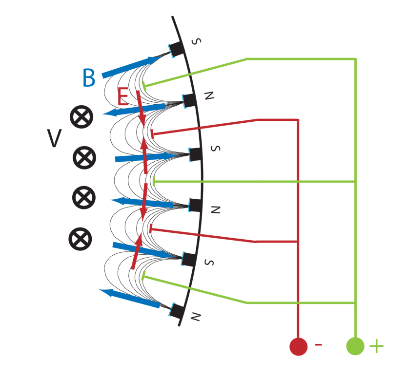
Figure 1: Partial vertical cross section of the proposed experiment. Rings of permanent magnets, of alternating polarity, line the inside of the sphere with their poles oriented radially. Ring anodes and cathodes lie between the magnets. The resulting $\mathbf{E}\boldsymbol{\times}\mathbf{B}$ drift is in the toroidal direction. By varying the potential between the anodes and cathodes the forcing at the outer boundary can be customized. The apparatus is axisymmetric.

Confinement in such a magnetic geometry has been well studied. Particle confinement is determined by ion-acoustic flows into the cusps, which can be modeled as a loss area equal to the linear dimension of the cusp times the ion gyroradius (Hershkowitz et al., 1975). Electrons are well confined by the cusp fields (Leung et al., 1976); their primary energy losses are through the cusp and through ion collisions. Ion energy confinement is mostly determined by charge exchange losses resulting from the relatively high fraction of neutrals in such devices. The ionization fraction of previous and current multidipole confinement systems varies considerably, but is typically $<$ 0.2.

Improved technology could allow the proposed experiment to exceed the confinement limits of earlier apparatuses. Modern NeFeB permanent magnets can generate cusp fields twice as strong as those in previous cylindrical experiments. This would result in lower loss rates, due to the narrowing of the cusps, and increased electron temperature, which has been shown to scale with cusp magnetic field strength (Ehlers & Leung, 1982). Heating of the plasma could be done using large area Lanthanum Hexaboride (LaB₆) cathodes. Such cathodes have previously been used in ion sources (Ehlers & Leung, 1979; Leung et al., 1984; Pincosy & Leung, 1985), and in a variety of plasma experiments (Ono et al., 1987; Darrow et al., 1990). These sources produce significantly more power than tungsten filaments, which would lead to higher temperatures and ionization fractions than previous devices.

To inject momentum into the experiment, ring anodes and cathodes are alternately placed between the ring magnets (Figure 1). These generate an electric field that causes an $\mathbf{E}\boldsymbol{\times}\mathbf{B}$ drift in the toroidal direction. The magnitude and direction of this drift can be varied as a function of angle by changing the electrical potential between the anodes and cathodes, allowing control over the fluid’s outer toroidal velocity field boundary condition. Viscous coupling between the magnetized and unmagnetized regions of the experiment is assumed.

A broad set of experimental regimes can be generated using such a device. Some of the specifications of the proposed experiment are listed in Table 1. In the context of this study, we are particularly interested in the magnetic Reynolds and Prandtl numbers. The magnetic Reynolds number for a plasma is given by

$$Rm=1.5\frac{T_{\rm e}^{3/2}Ua}{Z},$$ (1)

where the electron temperature, $T_{\rm e}$, is measured in electron volts, $U$ is the peak speed of the plasma in km s^-1, the length scale $a$ is measured in meters, and $Z$ is the charge of the ions. High electron temperatures, and the high speeds of plasmas, can lead to very large values of magnetic Reynolds number. In an unmagnetized plasma the viscosity is given by $\nu\sim V_{T{\rm i}}^{2}\tau_{\rm ei}$, where $V_{T{\rm i}}=2\sqrt{T_{\rm i}}{m_{\rm i}}$ is the thermal velocity of the ions, $\tau_{\rm ei}$ is the electron-ion collision time, $T_{\rm i}$ is the ion temperature and $m_{\rm i}$ is the ion mass. The unmagnetized magnetic Prandtl number is then

$$Pm=0.18\frac{T_{\rm e}^{3/2}T_{\rm i}^{5/2}}{\mu^{2}n},$$ (2)

where the ion temperature is measured in electron volts, $\mu$ is the atomic mass number of the ions, and $n$ is the number density in units of $10^{18}$ m^-3. The strong dependence on density and ion mass allows a very large range of magnetic Prandtl number, and by extension fluid Reynolds number, $Re=Rm/Pm$, allowing the experimenter the ability to specify whether a given plasma will be laminar or turbulent.

Table 1: Parameters of the Experiment

Quantity	Symbol	Value	Unit
plasma radius	$a$	1.5	m
number density	$n$	1017–1019	m-3
ion temperature	$T_{\rm i}$	0.5–4	eV
electron temperature	$T_{\rm e}$	2–10	eV
peak speed	$U_{\rm max}$	0–20	km s-1
ion species	H, He, Ar	1, 4, 40	amu
pulse length	$\tau_{\rm pulse}$	5	s
plasma beta	$\beta$	104
resistive time	$\tau_{\eta}$	50	ms
magnetic Reynolds number	$Rm_{\rm max}$	$\sim$ 1000–2000
Reynolds number	$Re$	2.4$\times$101–3.8$\times$106
magnetic Prandtl number	$Pm$	3.0$\times$10-4–5.6$\times$101

Varying density and ion mass to control the viscosity of the plasma is not without its tradeoffs, the primary one being the saturation level of the magnetic field generated by the dynamo, since it is dependant upon the kinetic energy of the fluid. Assuming that saturation occurs when the magnetic energy is in equipartition with the kinetic energy, $B^{2}/\mu_{0}=\rho U^{2}$, implies

$$B_{\rm equipartion}\approx 0.4\sqrt{\mu n}U\>\mbox{Gauss}.$$ (3)

At $T_{e}=10$ eV, $U=$ 20 km s^-1, $B_{\rm equipartion}$ could be as high as 240 Gauss with Ar at $n=10^{19}$ m^-3. However, as we will show in Section 3, simulations indicate that in saturation the magnetic field magnitude is not this high, but at best $B^{2}/\mu_{0}\simeq 0.1\rho U^{2}$.

The lack of magnetic field in the volume of the experiment and a method to control the velocity field means that this device should satisfy the criteria needed to create magnetically self-exciting plasmas. Its high value of $Rm$ and variable magnetic Prandtl number would allow it to be used to study physical regimes inaccessible to liquid-metal experiments. It would be the first plasma experiment used to study dynamos, though not the first to be proposed (Wang et al., 2002), and its wide range of parameters (Table 1) should allow it to be useful for the study of a number of other astrophysical phenomena: magnetorotational instability, high-$\beta$ instabilities and rotating convection, to name just a few. In the next section we present numerical simulations which demonstrate that this concept should succeed as a dynamo experiment. The other topics above will be examined in future work.

3 Numerical simulations

A comprehensive simulation of such a plasma experiment would consider both the electron and ion species, as well as include a careful treatment of the $\mathbf{E}\boldsymbol{\times}\mathbf{B}$ forcing at the outer boundary. As a first approximation, however, we treat the plasma as an incompressible single fluid. This is a justified approximation since the mean free path of the particles is much shorter than the system size, and sound waves are not relevant. The simulation solves the vorticity evolution and magnetic induction equations using a standard pseudospectral method based on spherical harmonics, truncated at maximum spherical harmonic degrees $\ell_{\rm max}$ and $m_{\rm max}$; details have been given previously (Bayliss et al., 2007; Reuter et al., 2008). The $\mathbf{E}\boldsymbol{\times}\mathbf{B}$ forcing is approximated as a toroidal velocity field non-zero no-slip boundary condition. An electrically-insulating outer boundary is assumed.

For the sake of brevity, here we restrict our attention to two values of magnetic Reynolds number, $Rm=300,2000$, where the magnetic Reynolds number is based on the peak speed of the toroidal outer boundary condition, which is unity in all simulations. We examine several values of $Pm$ to demonstrate that this experiment should be able to generate both laminar and turbulent dynamos. Future studies will examine other regimes of interest.

3.1 Toroidal boundary conditions

To demonstrate the flexibility of such an apparatus, four different axisymmetric steady-state velocity fields, generated using different outer boundary conditions with $Rm=300$ and $Pm=1.0$, are presented in Figure 2. The first, perhaps the simplest that can be generated in such a device, is a rigid-rotor-type azimuthal field. Such a velocity field can be used, in combination with the injection of light ions into a heavy plasma, to study rotating convection in plasmas. The second velocity field, Figure 2(b), is generated by a boundary condition that follows a $v_{\phi}\sim s^{-1}$ dependence for much of its angular extent, where $s$ is the cylindrical radial coordinate. The toroidal flow generated by this boundary does not have a $s^{-1}$ dependence, but rather is Keplerian for much of the volume of the sphere, with $v_{\phi}\sim s^{-1/2}$ at the equator, and as such should be unstable to the magnetorotational instability (MRI) (Balbus & Hawley, 1991). Not surprisingly, when this flow is exposed to an externally-applied magnetic field an MRI-like instability appears to develop.

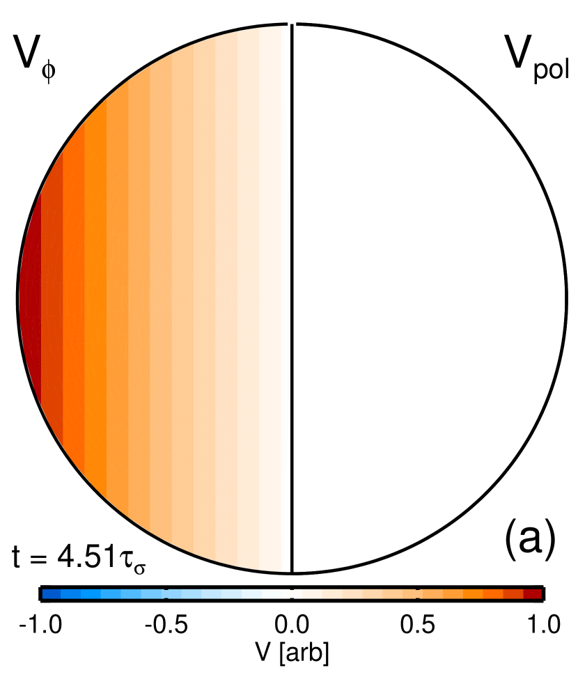
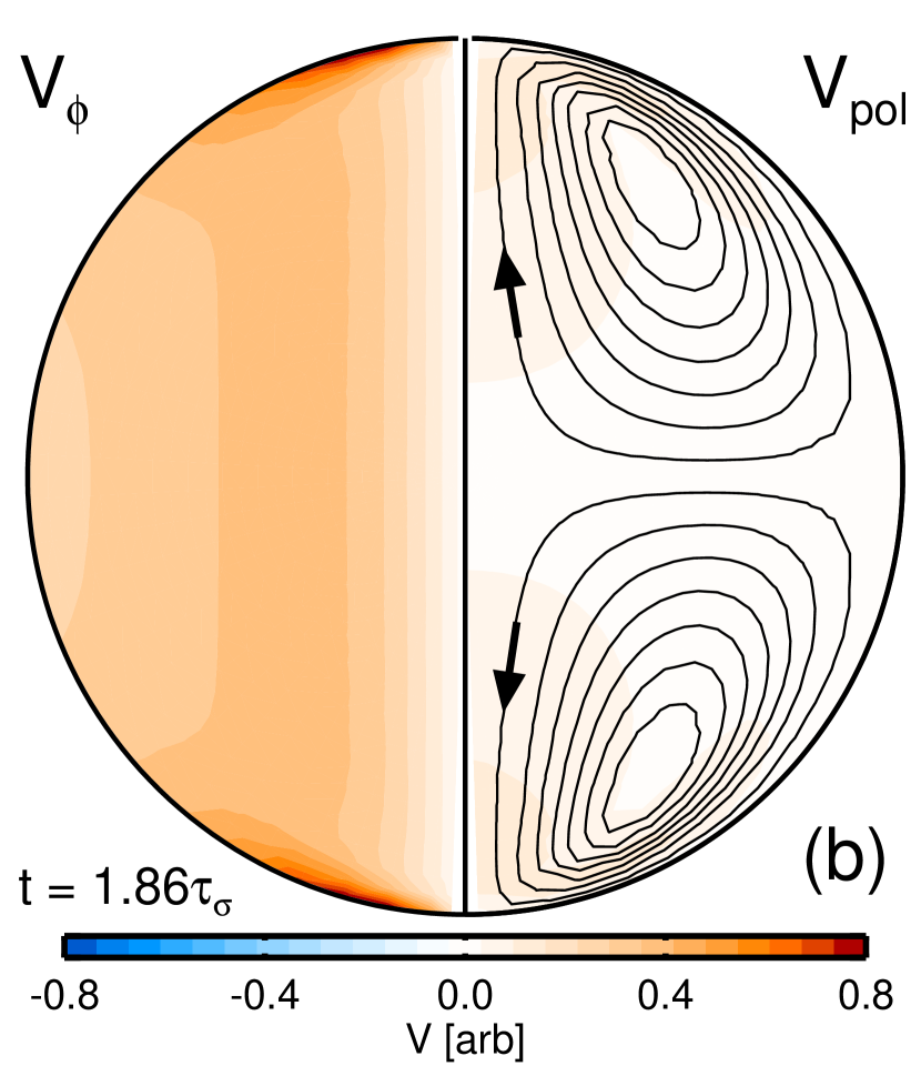
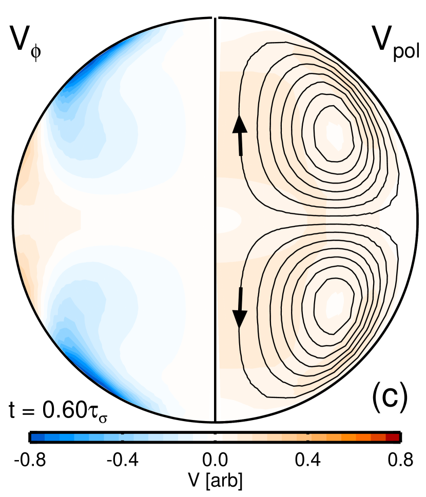
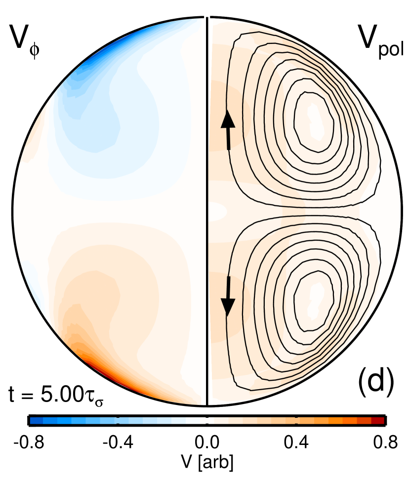
Figure 2: Steady-state axisymmetric velocity fields generated by different toroidal boundary conditions, with $Rm=300$ and $Pm=1.0$. The axis of symmetry runs vertically. In the left hemisphere are the contours of toroidal speed, and in the right hemisphere are the contours of the poloidal stream function. The boundary conditions are (a) solid-body rotation, which generates no poloidal flow (b) $v_{\phi}\sim s^{-1}$, which results in a Keplerian profile (c) equatorially symmetric, which results in dynamo action and (d) von Kármán (given in Figure 3), which also generates a dynamo. Note that, as indicated in Figure 3, the peak speed is set to 1.0, but the scale range in figures (b)-(d) has been reduced for clarity.

The velocity fields presented in Figures 2(c) and 2(d) are both magnetically unstable, displaying dynamo action under the conditions presented. The first boundary condition is equatorially symmetric, resulting in a flow with net kinetic helicity, while the second boundary condition is equatorially anti-symmetric. For the remainder of this paper we will focus on the second of these two cases, which is based on the von Kármán flow (von Kármán, 1921), a flow which has been extensively studied in the cylindrical geometry (Odier et al., 1998; Bourgoin et al., 2002, 2004). In this case the outer boundary rotates in opposite directions near the poles of the sphere and relatively little near the equator, as seen in Figure 3. The boundary condition is constructed from non-zero outer boundary values for the even-numbered axisymmetric spherical harmonic components $\ell=2,4,6,8$; these values, and all the boundary values used in this study, are given in Appendix A. This boundary condition results in laminar and turbulent dynamo action depending on the value of $Rm$ and $Re$ (for this boundary condition the transition to turbulence begins at $Re\sim 500$, depending on the level of forcing). The parameter values used in the simulations presented in this study, and exemplary physical values of corresponding plasmas, can be found in Table 2.

Table 2: Simulation Parameters & Plasma Values

			$T_{\rm e}$	$T_{\rm i}$	$U$	$n$		$B_{\rm max}$
$Rm$	$Pm$	$Re$	(eV)	(eV)	(km s-1)	(1018 m-3)	Ion	(G)	$N_{r}$	$\ell_{\rm max}$	$m_{\rm max}$
300	2.0	150	4.3	3.1	20.0	13.8	H	3.2	200	14	14
300	1.0	300	4.3	3.1	20.0	27.6	H	4.2	200	14	14
300	0.5	600	10.0	4.0	5.7	22.7	He		300	18	14
2000	1.0	2000	15.9	4.0	19.1	23.0	He	12.0	600	50	30

Note. — The radius of the unmagnetized plasma volume, $a$, is taken to be 1.1 m. $N_{r}$ is the number of radial grid points, equally spaced in the range $0<r\leq 1$. $B_{\rm max}$ refers to the maximum saturated magnetic field strength.

Figure 3: Toroidal boundary condition used in the simulations to generate a von Kármán-type flow. This boundary condition is constructed from the boundary values specified in Appendix A.

3.2 Laminar dynamo simulations

Among the many appealing features of the proposed experiment is its ability to create laminar MHD flows at very low values of fluid Reynolds number, something that is not possible with liquid-metal experiments. Though such flows are an imperfect analogy of naturally-occurring dynamos, since all natural flows are turbulent, their study can be used to test basic MHD under idealized conditions as well as the numerical codes which simulate them. Low-Reynolds-number flows can also be used to study the laminar-to-turbulent transition, and should allow the observation of the spontaneous relaminarization of a turbulent flow by a self-excited magnetic field (Bayliss et al., 2007). Here we restrict our examination to a set of laminar dynamos which could be generated in the proposed experiment.

It might come as a bit of a surprise that a laminar velocity field generated by a toroidal differentially-rotating outer boundary can generate a dynamo, since the poloidal component of the velocity field only results from Ekman circulation, making it difficult to achieve the balance of toroidal-to-poloidal flow needed for laminar dynamo action. Also, since the toroidal flow peaks at the edge of the sphere, the poloidal field is unable to easily stretch the magnetic field around the toroidal flow’s peak, and thus the stretch-twist-fold mechanism (Childress & Gilbert, 1995) that sustains laminar dynamos is much less efficient than that of other flows (Dudley & James, 1989). This manifests itself in the comparably large critical magnetic Reynolds number required for the toroidally-driven flows to self-excite.

The velocity field which results from the von Kármán boundary condition, with $Rm=300$ and $Pm=1.0$ (Figure 2(d)), is axisymmetric, counter-rotating in the toroidal direction, and has a poloidal flow which rolls inward at the equator and outward at the poles. As such the velocity field is qualitatively similar to the $s2t2$ flow of Dudley & James (1989), with the important distinction that the toroidal flow peaks at the sphere boundary. The magnetic and kinetic energies of this simulation, as a function of time in resistive units ($\tau_{\eta}=a^{2}/\eta$), are given in Figure 4. The growth rate of the magnetic energy is very small, symptomatic of the flow’s inefficiency as a dynamo. The critical magnetic Reynolds number for this flow, based on a linear stability analysis, is $Rm_{\rm crit}\simeq 237$. As is required for axisymmetric velocity fields by Cowling’s theorem (Cowling, 1933), the excited magnetic field is non-axisymmetric, dominated by $m=1$ modes; this is a large-scale dynamo. Overall the final magnetic field is weak, with the magnetic energy peaking an order of magnitude below the kinetic energy, resulting in minimal modification of the velocity field during saturation. The large-scale structure of the saturated magnetic field is given in Figure 5, demonstrating a geometry similar to other $s2t2$-type dynamo magnetic fields (Bayliss et al., 2007; Gissinger et al., 2008a, b; Reuter et al., 2009). Using the parameters in Table 2, the value of the magnetic field contour in Figure 5 is about 2 Gauss, which should be measurable in the proposed experiment using Hall-effect sensors.

Figure 4: Kinetic and magnetic energies versus time for the system forced by the boundary condition given in Figure 3, with $Rm=300$ and $Pm=0.5,1.0,2.0$. The kinetic energy for the three simulations is essentially the same. The $Pm=0.5$ simulation does not display dynamo action.

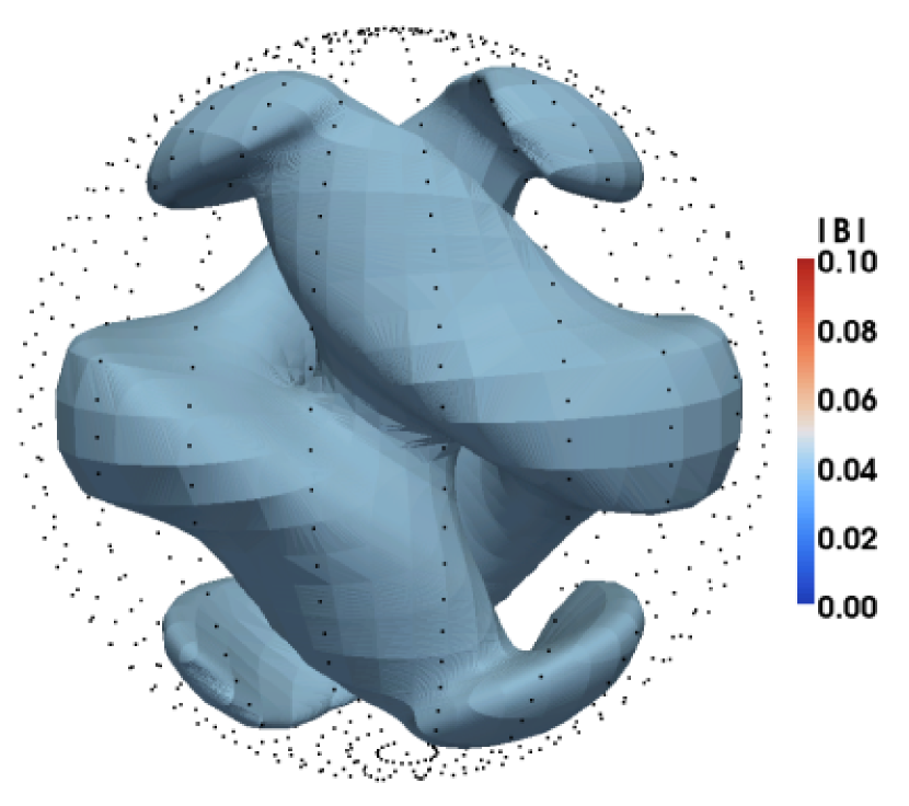
Figure 5: Contour of constant magnetic field magnitude during saturation, for the $Rm=300$, $Pm=1.0$ laminar dynamo. The axis of symmetry runs vertically.

The experimenter’s ability to vary the fluid’s magnetic Prandtl number can be used to explore the onset of turbulence and how that turbulence affects laminar dynamo action. The energies of two other simulations which use the boundary condition presented in Figure 3, with $Rm=300$ but with $Pm=2.0,0.5$ ($Re=150,600$), are plotted in Figure 4. For $Pm=2.0$, the boundary condition results in a velocity field that is magnetically unstable. This flow has a higher critical magnetic Reynolds number than the $Pm=1.0$ case, $Rm_{\rm crit}\simeq 274$, and consequently has a lower magnetic field growth rate, since as expected the growth rates are proportional to $Rm-Rm_{\rm crit}$. Interestingly, the magnetic field energy saturates at essentially the same value as the $Pm=1.0$ case, indicating that the saturated magnetic field does not follow the $B^{2}\sim(\rho\nu/\sigma a^{2})(Rm-Rm_{\rm crit})$ scaling, as might otherwise be expected (Petrelis & Fauve, 2001). The $Pm=0.5$ case does not magnetically self-excite, with the energy used to initialize the magnetic field modes quickly dissipating away. In this case the flow contains several non-axisymmetric, though stationary, components which interfere with the growth of the magnetic field. This underlying symmetry-breaking hydrodynamic instability is a first step towards developed turbulence, and as such permits the study of how non-axisymmetric contributions change the onset conditions for dynamo action.

3.3 Turbulent dynamo simulations

The question of the role of turbulence in the development and maintenance, or hindrance and destruction, of astrophysical magnetic fields is of ongoing importance. This is especially true in light of the recent turbulent-dynamo results from the VKS2 experiment (Monchaux et al., 2007) and the suggestion that coherent turbulence may be responsible for that dynamo (Laguerre et al., 2008). Clearly the proposed experiment will be most relevant to the study of astrophysical dynamos if it is able to generate self-excited magnetic fields under turbulent conditions.

To examine this question, simulations were performed at the higher end of the experiment’s expected range of magnetic Reynolds number, $Rm=2000$, with $Pm=1.0$ ($Re=2000$), using the toroidal outer boundary condition presented in Figure 3. The kinetic and magnetic energies of this simulation versus time are presented in Figure 6. The magnetic energy grows exponentially in time, saturating an order of magnitude below the kinetic energy. Using the parameters in Table 2, the magnetic field in saturation peaks as high as 12 Gauss. Since the magnetic field varies rapidly in time it should be easily measurable using B-dot coils.

Both the velocity and magnetic fields fluctuate wildly throughout the simulation. Snapshots of contours of $|\mathbf{B}|$ during saturation are presented in Figure 7. The transient nature of the magnetic field, and the lack of obvious large-scale structure at these contour levels, as compared to the large-scale dynamo (Figure 5), is clear. Nonetheless, the mean saturated magnetic field is non-zero; its energy is about 4% of the mean energy of the magnetic field in saturation, when averaged over 2.9 resistive times. Contours of the mean saturated magnetic field are presented in Figure 8. The field is somewhat complex, dominated by $m=0,1,2$ modes, and is weak at the center of sphere. The magnetic field at the sphere’s surface peaks at the equator, though it is composed of $m=1$ and $m=2$ components, in contrast to the large-scale dynamo, which only consists of $m=1$ modes.

Figure 6: Kinetic and magnetic energies versus time for the system forced by the boundary condition given in Figure 3, with $Rm=2000$ and $Pm=1.0$.

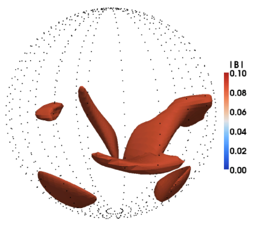
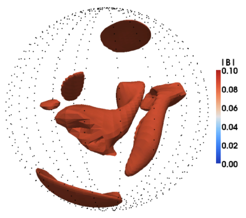
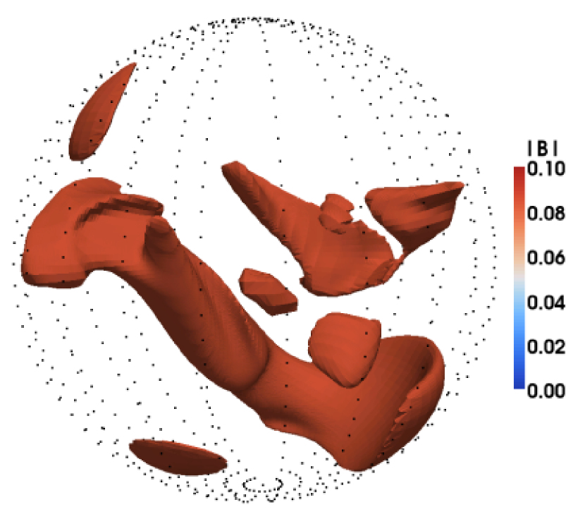
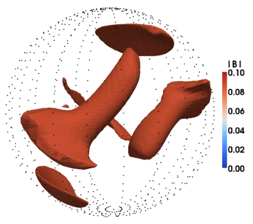
Figure 7: Contours of constant magnetic field magnitude for four different times during the saturation of the $Rm=2000$, $Pm=1.0$ turbulent dynamo. The figures are $\Delta t\simeq 0.2\tau_{\eta}$ apart in time.

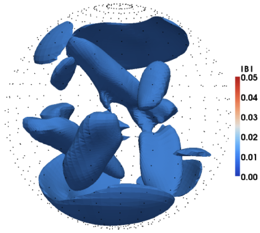
Figure 8: Contours of constant magnetic field magnitude for the $Rm=2000$, $Pm=1.0$ turbulent dynamo’s mean saturated magnetic field. The scale has been reduced from Figure 7 for clarity.

The growth rate of the magnetic field is much larger in this case than in the laminar cases examined above. This may be true because the system is much higher above the critical magnetic Reynolds number for this set of parameters, as compared to the laminar case, or because a different dynamo mechanism is at work, perhaps amplification at small scales. If the growth rate of the magnetic field were being dominated by turbulent action at small scales, following Batchelor (1950), we would expect the magnetic energy to grow exponentially in time as $\left|\mathbf{B}\right|^{2}\sim{\rm exp}((\epsilon Re)^{1/2}t)$, where $\epsilon$ is the power dissipation per unit mass. For this simulation $\epsilon\simeq 16$, so for the small-scale-dynamo mechanism we would expect the growth rate to be $\sim 180$, not the $\sim 40$ which is actually measured. The critical magnetic Reynolds number for this simulation has not yet been found, though we have determined that it is somewhere in the range $Rm<700$. Based on these observations, it seems unlikely that the action of small-scale eddies is the dominant contribution to the growth of magnetic energy, but rather since $Rm=2000$ the rapid growth rate is explained by the high magnetic Reynolds number.

To gain insight into the length scales important to this dynamo, we examine the average angle-integrated energy spectra of the velocity and magnetic fields, $E(k)$ and $M(k)$ respectively, where $M(k)=k^{2}\int\langle|\mathbf{B}(\mathbf{k})|^{2}\rangle d\Omega_{k}$, during the growth phase of the simulation, normalized to their respective total energies. These are plotted in Figure 9 (the details of how $\mathbf{B}(\mathbf{k})$ is calculated are given in Appendix B). The spectra have a number of interesting features. First, the velocity field spectrum is very noisy at higher values of $k$. This phenomenon is likely caused by the transform to $k$-space, which involves a radial integration across the edge of the sphere, where the velocity field quickly goes to zero (except for the toroidal boundary condition). Since the magnetic field does not go to zero at the sphere’s edge it does not display this effect. The velocity field spectrum peaks at relatively low wavenumber, as is expected since the energy in the simulation is being injected at the largest scales. The magnetic energy, in contrast, peaks at higher wavenumber and drops off rapidly. The general understanding of small-scale dynamos, at least for $Pm\sim 1$ and $Pm\gg 1$ (Schekochihin et al., 2004) is that the magnetic spectrum during the kinematic phase should peak at $k_{\eta}$, which for $Pm=1.0$ simulations should be the same as $k_{\nu}$, the knee in the velocity field spectrum. This is not the case in this situation, again suggesting that this is not a small-scale dynamo. Of course it is worth noting that the current understanding of the small-scale dynamo exists in the context of a number of assumptions, most notably those of homogeneous and isotropic turbulence and the lack of a mean flow; none of these assumptions apply in this situation.

Figure 9: Time-averaged, angle-integrated, kinematic magnetic and kinetic energy spectra, $M(k)$ and $E(k)$ respectively, for the $Rm=2000$, $Pm=1.0$ dynamo, normalized to their respect energies.

Though it has not been ruled out definitely, based on the growth rate of the magnetic energy, the non-zero mean saturated magnetic field, and the spectra of the kinematic magnetic field, we believe that the dynamo presented here is not a small-scale dynamo, but rather is an example of a turbulent large-scale dynamo. It is possible that this dynamo is related to some of the previously studied turbulent dynamos which possess a mean flow and similar magnetic spectra (Ponty et al., 2005; Mininni, 2006), or the recently-discovered ’shear dynamo’ (Yousef et al., 2008), though none of these studies were done in a finite domain.

4 Discussion and conclusions

The simulations of the proposed experiment presented here invoke a number of assumptions regarding the forcing at the plasma’s outer edge. Though we believe that these simulations capture the important physics of the experiment, the assumption that the forcing can be modeled using a continuous no-slip boundary condition is debatable. Clearly local effects caused by the discrete magnetic and electric fields are being ignored with this treatment. Future simulations of the experiment will endeavor to more accurately model the forcing by using the NIMROD code (Sovinec et al., 2004) to add two-fluid, compressible, and collisionless physics, including anisotropic and long-mean-free-path effects. Such additions may be especially important at lower values of magnetic Prandtl number, as one might expect the development of Stewartson layers (Stewartson, 1957) near the discrete areas of forcing, similar to effects found in cylindrical MRI experiments with differentially rotating upper and lower rings (Burin et al., 2006). One might also expect the plasma to transport cusp magnetic field into the volume of the sphere, a phenomena that has been observed with flowing liquid sodium (Volk et al., 2006). This effect could be important for rotating convection experiments, especially for the study of the physics of the tachocline (Miesch, 2005).

Since it has long been known that many axisymmetric flows exist which magnetically self-excite (Roberts, 1971; Gubbins, 1973; Dudley & James, 1989) it is expected that there are a multitude of boundary conditions which could be programmed into the experiment which would result in laminar dynamo action, allowing the study of the different means by which large-scale dynamos occur. Other boundary conditions which might be of interest include solar-type boundary conditions, where the equator spins much faster than the poles, and gas-giant-type boundary conditions, where the surface contains many prograde and retrograde jets. Density stratification and convection in rapidly rotating plasmas are also possible for this experiment, and should be studied.

The laminar dynamo presented in this study is large scale, as must be the case when there is no energy in the velocity field at small scales. As the fluid Reynolds number is increased the simulations become turbulent. As described in Section 3.3, the current understanding of the turbulent dynamo presented here is that it is not a small-scale dynamo, but rather a very turbulent large-scale dynamo. Because the outer toroidal boundary condition can be controlled in time, it is conceivable that a turbulent small-scale dynamo could be generated in this experiment without the presence of a mean flow. This is a topic which requires further study. Another question of considerable interest is: at what point does a large-scale dynamo become so turbulent that it ceases to have appreciable energy at the large scales and becomes small-scale? Does such a transition exist, or does the presence of a mean flow prevent this from happening? The proposed experiment, with its ability to reach high values of $Rm$ and wide range of kinetic Reynolds number, would be uniquely positioned to study these questions.

It is easily possible to reach $Pm\gg 1$ under laminar conditions, as been shown in many numerical simulations (Schekochihin et al., 2004). Another goal of the proposed experiment should be to attempt to study the $Pm\gg 1$ regime under fully turbulent conditions. This will be challenging, at least for the boundary condition examined here. The forcing strategy of the proposed experiment does not fill the volume of the fluid, but only affects the boundary, and thus a high value of $Re$ is needed to make the fluid turbulent. (A simulation was performed with $Rm=2000$ and $Re=1000$. This was laminar until saturation of the dynamo was achieved.) This need for a high value of fluid Reynolds number puts an upper limit on the experimental value of $Pm$ that can be reached under turbulent conditions. Those researchers that perform simulations of this physical regime suffer from a similar problem; for the simulators the problem is a lack of the resolution needed to reach high $Pm$ at high $Rm$, for the proposed experiment it is one of a technical upper limit on the value of magnetic Reynolds number that is experimentally accessible.

In summary, we have presented a concept for a high-$\beta$ plasma experiment which by its nature would be ideal for studying the MHD dynamo and a variety of astrophysical fluid dynamics phenomena, many of which have never been studied experimentally. The experiment’s plasma confinement is based on a ring-cusp strategy, and momentum is injected into the plasma via differential toroidal $\mathbf{E}\boldsymbol{\times}\mathbf{B}$ forcing at the plasma’s outer edge. With the advances in technology of the last few decades this experiment should be able to reach parameter regimes inaccessible to previous multidipole experiments. We have demonstrated through numerical simulations that such a control scheme is sufficient for generating velocity fields which are capable of both laminar and turbulent dynamo action. The combination of velocity-field tunability, high plasma $\beta$, and wide range of kinetic and magnetic Reynolds numbers would make this experiment a viable choice for exploring a multitude of astrophysical phenomena.

Appendix A Outer Boundary Values

The toroidal velocity field radial profile boundary values which are used to generate the results presented in this paper, and which are used to generate Figure 3, can be found in Table 3.

Table 3: Toroidal Boundary Values

$\ell$	Fig. 2(a)	Fig. 2(b)	Fig. 2(c)	Fig. 2(d)
1	0.5773	0.2273	-0.0667	0.0000
2	0.0000	0.0000	0.0000	-0.1002
3	0.0000	0.0541	-0.1234	0.0000
4	0.0000	0.0000	0.0000	-0.0788
5	0.0000	0.0239	-0.0130	0.0000
6	0.0000	0.0000	0.0000	-0.0110
7	0.0000	0.0124	0.0279	0.0000
8	0.0000	0.0000	0.0000	0.0117
9	0.0000	0.0067	0.0000	0.0000
11	0.0000	0.0036	0.0000	0.0000
13	0.0000	0.0018	0.0000	0.0000
15	0.0000	0.0008	0.0000	0.0000
17	0.0000	0.0002	0.0000	0.0000

It should be noted that the simulation code uses the following normalization for axisymmetric spherical harmonics:

$$Y_{\ell}^{0}(\theta,\phi)=\sqrt{(2\ell+1)}P_{\ell}^{0}(\cos\theta).$$ (A1)

This normalization affects the radial profile boundary values.

Appendix B Spatial Transforms

The simulation code evolves the velocity and magnetic fields in a spherical harmonic basis. To calculate $M(k)$ and $E(k)$ the fields must be transformed into spherical $k$ space. Rather than convert from the spherical harmonic basis to physical space, and then transform to $k$ space, the fields are transformed directly from the spherical harmonic basis to spherical $k$ space. This Appendix outlines how this is accomplished.

The native form of the fields is in terms of radial profiles projected onto a spherical harmonic basis, assuming that the fields are divergence free:

$$\mathbf{B}=\sum_{\alpha}\boldsymbol{\nabla}\boldsymbol{\times}\boldsymbol{\nabla}\boldsymbol{\times}\left[S_{\alpha}(r)Y_{\alpha}(\theta,\phi)\mathbf{r}\right]+\boldsymbol{\nabla}\boldsymbol{\times}\left[T_{\alpha}(r)Y_{\alpha}(\theta,\phi)\mathbf{r}\right],$$ (B1)

where we follow the convention of Moffatt (1978) and use a full $\mathbf{r}$ vector, as opposed to the convention of Bullard & Gellman (1954) who used the $\mathbf{\hat{r}}$ unit vector. The summation over $\alpha$ is over all valid spherical harmonic combinations, $\ell$ and $m$, starting at $\ell=1$, truncated at some $\ell_{\rm max}$ and $m_{\rm max}$. The radial profiles $S_{\alpha}(r)$ and $T_{\alpha}(r)$ are the profiles which characterize the field. Thus defined, the components of the field take the form

$$B_{r}(r,\theta,\phi) =\sum_{\alpha}\frac{\ell_{\alpha}(\ell_{\alpha}+1)S_{\alpha}(r)}{r}Y_{\alpha}(\theta,\phi),$$ (B2)

$$B_{\theta}(r,\theta,\phi) =\sum_{\alpha}\left[\frac{1}{r}\frac{\partial(rS_{\alpha}(r))}{\partial r}\frac{\partial Y_{\alpha}}{\partial\theta}+\frac{T_{\alpha}(r)}{\sin\theta}\frac{\partial Y_{\alpha}}{\partial\phi}\right],$$ (B3)

$$B_{\phi}(r,\theta,\phi) =\sum_{\alpha}\left[-T_{\alpha}(r)\frac{\partial Y_{\alpha}}{\partial\theta}+\frac{1}{r\sin\theta}\frac{\partial(rS_{\alpha}(r))}{\partial r}\frac{\partial Y_{\alpha}}{\partial\phi}\right].$$ (B4)

We now desire

$$\mathbf{B}(\mathbf{k})=\frac{1}{(2\pi)^{3/2}}\int e^{i\mathbf{k}\cdot\mathbf{x}}\mathbf{B}(\mathbf{x})d\mathbf{x}=\frac{1}{(2\pi)^{3/2}}\int e^{ikr\cos\gamma}\mathbf{B}(\mathbf{x})r^{2}dr\sin\theta d\theta d\phi,$$ (B5)

where $\cos\gamma=\sin\theta_{k}\sin\theta\cos\left(\phi-\phi_{k}\right)+\cos\theta_{k}\cos\theta$. Calculation of this integral requires several identities. We will use the Rayleigh equation,

$$e^{ikr\cos\gamma}=\sum_{n=0}^{\infty}i^{n}\left(2n+1\right)j_{n}(kr)P_{n}(\cos\gamma),$$ (B6)

where $j_{n}(kr)$ is the spherical Bessel function of the first kind, and $P_{n}(\cos\gamma)$ is the Legendre polynomial. This expansion over $n$ is truncated at $\ell_{\rm max}$, which gives satisfactory convergence for the cases considered here. We also need the addition theorem for spherical harmonics,

$$P_{n}(\cos\gamma)=\sum_{m=0}^{m=n}\frac{4\pi}{2n+1}Y_{n}^{m\ast}(\theta,\phi)Y_{n}^{m}(\theta_{k},\phi_{k}).$$ (B7)

We first consider the radial component of this transform. Combining equations B2, B5, B6 and B7 gives

$$B_{k}(k,\theta_{k},\phi_{k})=\frac{2}{\sqrt{2\pi}}\sum_{n=1}^{\ell_{\rm max}}\sum_{m=0}^{m=n}i^{n}n\left(n+1\right)Y_{n}^{m}(\theta_{k},\phi_{k})\int_{0}^{\infty}j_{n}(kr)S_{n}^{m}(r)rdr,$$ (B8)

where orthonormality between the spherical harmonics has been assumed. The $\theta_{k}$ and $\phi_{k}$ components of the transform are a little more complicated. Let us consider the first term on the right hand side of equation B3. If the spherical harmonics are defined as $Y_{\alpha}(\theta,\phi)=N_{\alpha}P_{\ell_{\alpha}}^{m_{\alpha}}(\cos\theta)e^{im_{\alpha}\phi}$, where $N_{\alpha}$ is the normalization constant, then the contribution from the first term is given by

$$B_{\theta_{k}}(k,\theta_{k},\phi_{k})_{\rm 1^{\rm st}}=\frac{4\pi}{\sqrt{2\pi}}\sum_{n=0}^{\ell_{\rm max}}\sum_{\ell_{\alpha}=1}^{\ell_{\rm max}}\sum_{m=0}^{m=n} N_{n}N_{\alpha}i^{n}Y_{n}^{m}(\theta_{k},\phi_{k})\int_{0}^{\infty}j_{n}(kr)\frac{\partial(rS_{\ell_{\alpha}}^{m})}{\partial r}rdr\times$$

$$\int_{0}^{\pi}P_{n}^{m}(\cos\theta)\frac{\partial P_{\ell_{\alpha}}^{m}(\cos\theta)}{\partial\theta}\sin\theta d\theta.$$ (B9)

The second term is similar:

$$B_{\theta_{k}}(k,\theta_{k},\phi_{k})_{\rm 2^{\rm nd}}=\frac{4\pi}{\sqrt{2\pi}}\sum_{n=0}^{\ell_{\rm max}}\sum_{\ell_{\alpha}=1}^{\ell_{\rm max}}\sum_{m=0}^{m=n} N_{n}N_{\alpha}i^{n+1}mY_{n}^{m}(\theta_{k},\phi_{k})\int_{0}^{\infty}j_{n}(kr)T_{\ell_{\alpha}}^{m}(r)r^{2}dr\times$$

$$\int_{0}^{\pi}P_{n}^{m}(\cos\theta)P_{\ell_{\alpha}}^{m}(\cos\theta)d\theta.$$ (B10)

The terms needed to calculate $B_{\phi_{k}}$ are similar, the only differences being the quantities in the radial integrals.

It should be observed that the radial integral is evaluated all the way to infinity. For transforms of the velocity field, this integral is only evaluated up to $r=1$, since that is where the radial profiles go to zero, with the exception of the toroidal radial profiles which have non-zero boundary conditions. (This truncation of the radial profile at $r=1$ is what gives the velocity field spectra their spiky nature at high $k$. See Figure 9 for an example.) The radial integrals over $S_{\alpha}(r)$ are evaluated all the way to infinity, since the poloidal radial profiles are non-zero outside the sphere. Since the region $r>1$ is current-free, the radial profile is matched to the vacuum solution for the magnetic field. The external part of the radial integrals then become

$$\int_{1}^{\infty}j_{n}(kr)S_{n}^{m}(r)rdr =S_{n}^{m}(1)\int_{1}^{\infty}j_{n}(kr)r^{-n}dr,$$ (B11)

$$\int_{1}^{\infty}j_{n}(kr)\frac{\partial(rS_{\ell_{\alpha}}^{m}(r))}{\partial r}rdr =-\ell_{\alpha}S_{\ell_{\alpha}}^{m}(1)\int_{1}^{\infty}j_{n}(kr)r^{-\ell_{\alpha}}dr,$$ (B12)

the former integral being a special case of the latter. These integrals don’t change, and so have been tabulated for repeated use. The toroidal part of the magnetic field, $T_{\alpha}(r)$, like the velocity field radial profiles, goes to zero at $r=1$, since we are assuming an insulating outer boundary. Thus, the radial integrals over $T_{\alpha}(r)$ are only evaluated up to $r=1$.

References

- Balbus & Hawley (1991) Balbus, S. A. & Hawley, J. F. 1991, AJ, 376, 214
- Batchelor (1950) Batchelor, G. K. 1950, Proc. R. Soc. Lond., Ser. A, 201, 405
- Bayliss et al. (2007) Bayliss, R. A., Forest, C. B., Nornberg, M. D., Spence, E. J., & Terry, P. W. 2007, Phys. Rev. E, 75, 026303
- Bourgoin et al. (2002) Bourgoin, M., et al. 2002, Phys. Fluids, 14, 3046
- Bourgoin et al. (2004) Bourgoin, M., Volk, R., Frick, P., Khripchenko, S., Odier, P., & Pinton, J.-F. 2004, Magnetohydrodynamics, 40, 3
- Bullard & Gellman (1954) Bullard, E. C. & Gellman, H. 1954, Philos. Trans. R. Soc. Lond., Ser. A, 247, 213
- Burin et al. (2006) Burin, M. J., Ji, H., Schartman, E., Cutler, R., Heitzenroeder, P., Lui, W., Morris, L., & Raftopolous, S. 2006, Exp. in Fluids, 40, 962
- Childress & Gilbert (1995) Childress, S. & Gilbert, A. 1995, Stretch, Twist, Fold: The fast dynamo (Berlin: Springer-Verlag Telos)
- Cho et al. (1988) Cho, M. H., Hershkowitz, N., & Intrator, T. 1988, J. Vac. Sci. & Tech. A, 6, 2978
- Cowling (1933) Cowling, T. G. 1933, MNRAS, 94, 39
- Darrow et al. (1990) Darrow, D., et al. 1990, Phys. Fluids B: Plasma Phys., 2, 1415
- Dudley & James (1989) Dudley, M. L. & James, R. W. 1989, Proc. R. Soc. Lond., Ser. A, 425, 407
- Ehlers & Leung (1979) Ehlers, K. W., & Leung, K. N. 1979, Rev. Sci. Inst., 50, 1353
- Ehlers & Leung (1982) Ehlers, K. W., & Leung, K. N. 1979, Rev. Sci. Inst., 53, 1429
- Forest et al. (2002) Forest, C. B., Bayliss, R. A., Kendrick, R. D., Nornberg, M. D., O’Connell, R., & Spence, E. J. 2002, Magnetohydrodynamics, 38, 107
- Forest et al. (2008) Forest, C., Bayliss, A., Schnack, D., Spence, E., & Reuter, K. 2008, in Bulletin of the American Physical Society, Vol. 53, number 14, American Physical Society, 222
- Gailitis et al. (2000) Gailitis, A., et al. 2000, Phys. Rev. Lett., 84, 4365
- Gissinger et al. (2008a) Gissinger, C., Dormy, E., & Fauve S. 2008, Phys. Rev. Lett., 101, 144502
- Gissinger et al. (2008b) Gissinger, C., Iskakov, A., Fauve, S., & Dormy, E. 2008, Europhysics Lett., 82, 29001
- Gubbins (1973) Gubbins, D. 1973, Philos. Trans. R. Soc. Lond., Ser. A, 274, 493
- Haugen et al. (2004) Haugen, N. E. L., Brandenburg, A., & Dobler, W. 2004, Phys. Rev. E, 70, 016308
- Hershkowitz et al. (1975) Hershkowitz, N., Leung, K. N., & Romesser, T. 1975, Phys. Rev. Lett., 35, 277
- Iskakov et al. (2007) Iskakov, A. B., Schekochihin, A. A., Cowley, S. C., McWilliams, J. C., & Proctor, M. R. 2007, Phys. Rev. Lett., 98, 208501
- Kinney et al. (2000) Kinney, R. M., Chandran, B., Cowley, S., & McWilliams, J. C. 2000, ApJ, 545, 907
- Kulsrud (1999) Kulsrud, R. M. 1999, ARA&A, 37, 37
- Laguerre et al. (2008) Laguerre, R., Nore, C., Ribeiro, A., Léorat, J., Guerond, J.-L., & Plunian, F. 2008, Phys. Rev. Lett., 101, 104501
- Lang & Hershkowitz (1978) Lang, A. & Hershkowitz, N. 1978, J. Appl. Phys., 49, 4707
- Leung et al. (1976) Leung, K. N., Hershkowitz, N., & MacKenzie, K. R. 1976, Phys. Fluids, 19, 1045
- Leung et al. (1984) Leung, K. N., Pincosy, P. A., & Ehlers, K. W. 1984, Rev. Sci. Inst., 55, 1064
- Limpaecher & MacKenzie (1973) Limpaecher, R. & MacKenzie, K. R. 1973, Rev. Sci. Inst., 44, 726
- Miesch (2005) Miesch, M. S. 2005, Living Rev. Solar Phys., 2, 1, http://www.livingreviews.org/lrsp-2005-1
- Mininni (2006) Mininni, P. D. 2006, Phys. Plasmas, 13, 056502
- Moffatt (1978) Moffatt, H. K. 1978, Magnetic field generation in electrically conducting fluids (Cambridge, England: Cambridge University Press)
- Monchaux et al. (2007) Monchaux, R., et al. 2007, Phys. Rev. Lett., 98, 044502
- Odier et al. (1998) Odier, P., Pinton, J.-F., & Fauve, S. 1998, Phys. Rev. E, 58, 7397
- Ono et al. (1987) Ono, M., Greene, G., Darrow, D., Forest, C. B., Park, H., & Stix, T. 1987, Phys. Rev. Lett., 59, 2165
- Pelletier et al. (1984) Pelletier, J., Arnal, Y., Debrie, R., Pomathiod, L., & Rifflet, J. C. 1984, Rev. Sci. Inst., 55, 1636
- Petrelis & Fauve (2001) Pétrélis, F. & Fauve, S. 2001, European Phys. J. B, 22, 273
- Pincosy & Leung (1985) Pincosy, P. A. & Leung, K. N. 1985, Rev. Sci. Inst., 56, 655
- Ponty et al. (2005) Ponty, Y., Mininni, P. D., Montgomery, D. C., Pinton, J.-F., Politano, H., & Pouquet, A. 2005, Phys. Rev. Lett., 94, 164502
- Ravelet et al. (2005) Ravelet, F., Chiffaudel, A., Daviaud, F., & Léorat, J. 2005, Phys. Fluids, 17, 117104
- Reuter et al. (2009) Reuter, K., Jenko, F., & Forest, C. B. 2009, New J. Phys., 11, 013027
- Reuter et al. (2008) Reuter, K., Jenko, F., Forest, C. B., & Bayliss, R. A. 2008, Comp. Phys. Comm., 179, 245
- Roberts (1971) Roberts, G. O. 1971, in World magnetic survey 1957–1969, ed. A. J. Zmuda (Paris: International Union of Geodesy and Geophysics Publication Office), 123–131, reported by P. H. Roberts
- Schekochihin et al. (2002) Schekochihin, A. A., Maron, J. L., Cowley, S., & McWilliams, J. C. 2002, ApJ, 576, 806
- Schekochihin et al. (2004) Schekochihin, A. A., Cowley, S. C., Taylor, S. F., Maron, J. L., & McWilliams, J. C. 2004, ApJ, 612, 276
- Schekochihin et al. (2007) Schekochihin, A. A., Iskakov, A. B., Cowley, S. C., McWilliams, J. C., Proctor, M. R. E., & Yousef, T. A. 2007, New J. Phys., 9, 300
- Sovinec et al. (2004) Sovinec, C., et al. 2004, J. Comp. Phys., 195, 355
- Stewartson (1957) Stewartson, K. 1957, J. Fluid Mech., 3, 17
- Stieglitz & Müller (2001) Stieglitz, R. & Müller, U. 2001, Phys. Fluids, 13, 561
- Volk et al. (2006) Volk, R., et al. 2006, Phys. Rev. Lett., 97, 074501
- von Kármán (1921) von Kármán, T. 1921, Z. Angew. Math. & Mech., 93, 233
- Wang et al. (2002) Wang, Z., Pariev, V. I., Barnes, C. W., & Barnes, D. C. 2002, Phys. Plasmas, 9, 1491
- Yousef et al. (2008) Yousef, T. A., Heinemann, T., Schekochihin, A. A., Kleeorin, N., Rogachevskii, I., Iskakov, A. B., Cowley, S. C., & McWilliams, J. C. 2008, Phys. Rev. Lett., 100, 184501