Climbing Down from the Top:
Single Name Dynamics in Credit Top Down Models
Igor Halperin and Pascal Tomecek
Quantitative Research, JP Morgan
September 1, 2008

Abstract:

In the top-down approach to multi-name credit modeling, calculation of singe name sensitivities appears possible, at least in principle, within the so-called random thinning (RT) procedure which dissects the portfolio risk into individual contributions. We make an attempt to construct a practical RT framework that enables efficient calculation of single name sensitivities in a top-down framework, and can be extended to valuation and risk management of bespoke tranches. Furthermore, we propose a dynamic extension of the RT method that enables modeling of both idiosyncratic and default-contingent individual spread dynamics within a Monte Carlo setting in a way that preserves the portfolio “top”-level dynamics. This results in a model that is not only calibrated to tranche and single name spreads, but can also be tuned to approximately match given levels of spread volatilities and correlations of names in the portfolio.

1 Introduction

Modeling of a dynamic credit portfolio can proceed according to two different paradigms. In a bottom-up approach, we start with single name dynamics which are constructed to fit individual credit spreads. At the second stage, one attempts to calibrate the dependence structure (introduced via common factors or a copula) to portfolio pricing data such as tranche prices. However, calibration to tranches across multiple strikes and maturities can be quite challenging in this framework. Furthermore, the bottom-up approach makes it difficult (though not impossible, see Collin-Dufresne et al (2003) [1] and Schönbucher (2003) [2]) to introduce default clustering (contagion) in a tractable way.

In many applications, the portfolio loss (or spread-loss) process is all we need for pricing and risk management. In particular, this is the case when one wants to price a non-standard index tranche off standard ones, and risk-manage it using the same standard tranches plus the credit index. Another example is an exotic portfolio derivative (such as e.g. a tranche option) that is hedged using tranches written on the same portfolio. In recognition of this fact, the alternative, top-down approach, suggested by Giesecke and Goldberg (GG) (2005) [3], suggests that a portfolio-level (or economy-level) loss process, rather than loss processes for individual names, should be the modeling primitive. Such a process is generally much easier to calibrate to tranche prices than an aggregate portfolio loss process obtained with the bottom-up approach. Moreover, credit contagion is built-in in this approach by construction [3, 4]. Once a calibrated portfolio loss process is obtained, it can be used to price vanilla and exotic derivatives referencing the same portfolio. (For a further comparison between the bottom-up vs top-down paradigms and a brief review of published models, see e.g. Bielecki, Crépey and Jeanblanc [5] and references therein.)

The two alternative approaches to modeling credit portfolios, i.e. the bottom-up and top-down paradigms, are somewhat complimentary in the sense that typically, for practical applications we chose one of them based on its appropriateness as well as practicality of its use. If we are interested in pricing (and/or risk management using only a credit index and its tranches), then a transition to a coarse-grained description of the top-down approach can be justified, as eventually our payoffs are only functions of portfolio-level losses, not of losses on individual names. Note, however, that the knowledge of the portfolio loss process is not sufficient in more complicated (but common) situations, e.g. when a risk manager chooses to use single names for hedging. Hedging on a single name basis is often done for names in the portfolio whose spreads significantly widen. Obviously, calculation of single name sensitivities is beyond the reach of a model whose only output is a portfolio-level loss process.

In addition to the hedging issue, there exists another reason why single name calibration can be of substantial practical interest, which is the so-called “bespoke problem”. The problem is that most exotic portfolio credit derivatives (forward-starting tranches, tranche options, etc) reference customized (bespoke) portfolios, rather than standardized index portfolios. If we work with a top-down model, we have to calibrate it to tranches referencing this bespoke portfolio. However, such portfolios usually do not have enough liquidity, which forces practitioners to mark prices of tranches on bespoke portfolios off tranche quotes for index portfolios, using some sort of a mapping between the two portfolios. Currently, the market standard is to use the base correlation methodology along with an adjustment to the difference in expected portfolio losses between the two portfolios. However, this procedure is quite ad hoc and is neither consistent nor satisfactory. In particular, it often violates no-arbitrage conditions, thus posing substantial practical difficulties.

The bottom-up approach suggests, in principle, a natural method to deal with the bespoke problem: once a model is calibrated to market data at both the single name and tranche levels, arbitrary bespoke tranches can be priced with the same model by first choosing parameters obtained by calibration to index tranche prices for names that are common for the bespoke and index portfolios, and then relying on interpolation/extrapolation for names that are not. However, this argument can also be applied to a top-down model once we can calibrate it to single names in addition to tranches. In this case, the bespoke problem would be resolved in the top-down approach in exactly the same way as in the bottom-up approach.

With the top-down approach, information about single names can be recovered, at least in principle, using the so-called random thinning (RT) procedure proposed by Giesecke and Goldberg (2005) [3]. The idea of this approach is to allocate fractions of portfolio default intensity calibrated within the “top” part of the model to individual names in such a way that individual CDS spreads of names in the portfolio are matched. Once this is done, the model becomes calibrated to both tranche and single name data. Various versions of the RT discussed in [3, 4, 6] use thinning of the portfolio intensity by deterministic or piecewise-deterministic (ones that jump upon defaults in the portfolio) processes. (This involves a number of subtle technical points, see BCJ [5] and also below in Sect.2.3.)

In this paper, we take a probabilistic view of the problem of construction of single name dynamics within the top-down framework. Note that the “top” part of a top-down model can be viewed as producing “incomplete information” scenarios that yield a forecast of the timing of sequential defaults in the portfolio, but lose information on the defaulters’ identities. In a sense, our problem thus becomes a problem of inference, where we probabilistically assign identities to all future defaulters. As will be clear in what follows, our approach bears resemblance to the well-known statistical problem of inference of a two-dimensional (2D) probability distribution when only its 1D marginals (corresponding, in our case, to portfolio-level and individual names default forecasts, respectively) are known.

The contribution of this paper is two-fold. First, we present a practical RT framework that enables efficient calculation of single name sensitivities in a top-down framework, and can be extended to valuation and risk management of bespoke tranches. Second, we suggest a way of extending this framework to model dynamics of single names in a way that preserves both the portfolio-level calibration and dynamics. This is achieved by formulating and solving the problem of single name dynamics as a filtering problem. We construct an ”information process” to explicitly model the market filtration, and further show how parameters of this process could be chosen to approximately (in the portfolio-averaged sense) calibrate to a given set of single name spread volatilities and correlations. We note in this relation that most, if not all, of credit portfolio models usually concentrate on matching individual CDS spreads of names in a portfolio as well as tranche spreads, but not finer characteristics such as spread volatility. However, it can be expected that better control of spread dynamics might be important for the pricing and risk management of exotic portfolio credit derivatives. The particular framework employed in our construction does allow one to have some control of single name spread dynamics, which thus might be seen as an attractive feature of the top-down approach.

The paper is organized as follows. In Sect.2 we introduce the so-called top-down (TD) matrices which serve as the basic modeling primitives of our approach. Sect.3 then introduces the iterative scaling algorithm for calculation TD-matrices calibrated to single names. In Sect.4 we calculate single name sensitivities with our approach. Sect.5 describes the dynamics extension of our RT framework. A very short Sect.6 summarizes the numerical Monte Carlo algorithm for simulation single name dynamics. In Sect.7 we outline a method of approximate calibration of parameters driving the single name dynamics. The final Sect.8 presents some discussion and conclusions.

2 Top-down default time matrices

The following notation will be used throughout this paper:

• $\tau_{i}$ - default time of name $i$

• $\tau^{j}$ - time of the $j$-th default in the portfolio

• $[T^{(1)},\ldots,T^{(M)}]$ - reference maturities. We set $T^{(0)}=0$.

Next, we introduce our modeling primitives. For each interval $m=1,\ldots,M$, we consider the following matrix

$$P_{ij}^{(m)}(t)=P\left[\left\{\tau^{j}=\tau_{i}\right\}\bigcap\left\{T^{(m-1)}\leq\tau_{i}\leq T^{(m)}\right\}|\mathcal{F}_{t}\right].$$ (1)

In words, this is the joint probability that the $i$-th name is the $j$-th defaulter, and this event happens in the interval $[T^{(m-1)},T^{(m)}]$, conditional on the currently available information $\mathcal{F}_{t}$. (Modeling of filtration $\mathcal{F}_{t}$ will be discussed below.) Note that we assume instantaneous multiple default events are not possible. Clearly, we can equivalently write (1) as

$$P_{ij}^{(m)}(t)=P\left[\left.\left\{\tau_{i}=\tau^{j}\right\}\bigcap\left\{T^{(m-1)}\leq\tau^{j}\leq T^{(m)}\right\}\right|\mathcal{F}_{t}\right].$$ (2)

In what follows, we will occasionally refer to (1) or (2) as Top-Down default time matrices, or TD-matrices for short. The definitions (1), (2) are inspired by the formalism used in the reliability theory and competing risks models, where the object of inference is the joint probability $p(T,O)$ of the event $T$ (e.g. a first failure in a system) and the type $O$ of risk among a set of alternatives $O_{1},O_{2},\ldots$ that could cause the failure. In our setting, identities of defaulted names serve as risk types $O_{i}$, with an additional rule that they cannot repeat in the default history of a portfolio.

Both the single name and portfolio probabilities are obtained by marginalization:

$$\sum_{i}P_{ij}^{(m)}(t) = P\left[\left.T^{(m-1)}\leq\tau^{j}\leq T^{(m)}\right|\mathcal{F}_{t}\right],$$

$$\sum_{j}P_{ij}^{(m)}(t) = P\left[\left.T^{(m-1)}\leq\tau_{i}\leq T^{(m)}\right|\mathcal{F}_{t}\right],$$ (3)

where we used (2) and (1), respectively. Both the “top-down” and “bottom-up” forward probabilities entering the RHS of Eqs.(2) can be easily calculated as follows:

$$P\left[\left.T^{(m-1)}\leq\tau^{j}\leq T^{(m)}\right|\mathcal{F}_{t}\right] = w_{t}^{(m)}(j)-w_{t}^{(m-1)}(j),$$

$$P\left[\left.T^{(m-1)}\leq\tau_{i}\leq T^{(m)}\right|\mathcal{F}_{t}\right] = Q_{i,t}^{(m)}-Q_{i,t}^{(m-1)},$$ (4)

where $w_{t}^{(m)}(j)$ is the tail probability of having at least $j$ defaults in the portfolio by time $T^{(m)}$ (note that $w_{0}^{(0)}(j)=\delta_{j0}$), and $Q_{i,t}^{(m)}$ is the cumulative default probability of the $i$-th name by time $T^{(m)}$. Note that we explicitly show dependence on $t$ for both $w_{t}^{(m)}(j)$ and $Q_{i,t}^{(m)}$ to emphasize their dependence on the filtration $\mathcal{F}_{t}$.

2.1 Dynamics of TD matrices

The TD matrices are dynamic because we condition on the currently available information $\mathcal{F}_{t}$. In fact, from their definition it is clear that for any $i,j,m$, $P_{ij}^{(m)}(t)$ is a martingale in the filtration $(\mathcal{F}_{t})_{t\geq 0}$. In the remainder of this Section, as well as Sections 3 and 4, we examine the TD matrices as seen at time zero, i.e. conditional on $\mathcal{F}_{0}$. In Section 5, we show how the TD matrices are updated conditional on the information in $(\mathcal{F}_{t})_{t\geq 0}$. This must be done in a way that preserves the equations (2) and (2) as well as the martingale property.

The primary filtration $(\mathcal{F}_{t})_{t\geq 0}$ is constructed from the following definitions:

• $(\mathcal{G}_{t})_{t\geq 0}$ is the natural filtration of the top-down default-counting process: $\mathcal{G}_{t}=\sigma(\{\tau^{j}<t\};j=1,\ldots,N)$

• $(\mathcal{I}_{t})_{t\geq 0}$ is the filtration generated by the defaulters’ identities: $\mathcal{I}_{t}=\sigma(\{\tau^{j}=\tau_{i},\tau^{j}<t\};i,j=1,\ldots,N)$ (this will be obtained by simulation, see Sects. 2.3 and 5.1 below)

• $(\mathcal{H}_{t})_{t\geq 0}$ is a background filtration containing external market information, and possibly generated by several “information processes”

• The filtrations $(\mathcal{G}_{t})_{t\geq 0}$, $(\mathcal{I}_{t})_{t\geq 0}$, and $(\mathcal{H}_{t})_{t\geq 0}$ are assumed to be independent, and the filtration $(\mathcal{F}_{t})_{t\geq 0}$ is defined by

  $$\mathcal{F}_{t}=\mathcal{G}_{t}\vee\mathcal{I}_{t}\vee\mathcal{H}_{t}.$$ (5)

According to these definitions, the ordered default times $\tau^{j}$ are $\mathcal{G}$-stopping times, but the single name default times $\tau_{i}$ are typically not. However, both $\tau^{j}$ and $\tau_{i}$ are $\mathcal{F}$-stopping times.

The market filtration $\mathcal{H}$ is similar to that introduced by Brody, Hughston and Macrina (BHM) [8], which they use to introduce bond price dynamics to their model. In their paper, the filtration is generated by a Brownian bridge. By including this information in our overall filtration $\mathcal{F}$, we use similar techniques to enrich the dynamics of $P_{ij}^{(m)}(t)$ (see Section 5). In particular, by enlarging the filtration of interest, we are able to de-correlate (to a certain extent) the individual forward default probabilities from the index’s; without it, they would be perfectly correlated.

2.2 Relation to conditional forward matrices

Note that for $m=1$, our TD matrix $P_{ij}^{(1)}$ is simply related to a time-independent matrix $p_{ij}$ introduced by Ding, Giesecke and Tomecek [6] as a matrix of conditional probabilities, provided we restrict it to the time horizon given by $T^{(1)}$, $p_{ij}\rightarrow p_{ij}^{(1)}(t)\equiv P\left[\tau^{j}=\tau_{i}|\tau^{j}<T^{(1)},\mathcal{F}_{t}\right]$. Indeed, in this case we obtain

$$P_{ij}^{(1)}(t) = P\left[\left\{\tau^{j}=\tau_{i}\right\}\bigcap\left\{0\leq\tau^{j}\leq T^{(1)}\right\}|\mathcal{F}_{t}\right]$$

$$= P\left[\tau^{j}=\tau_{i}|\tau^{j}\leq T^{(1)},\mathcal{F}_{t}\right]\,P\left[\tau^{j}\leq T^{(1)}|\mathcal{F}_{t}\right]\equiv p_{ij}^{(1)}(t)w^{(1)}_{t}(j).$$

On the other hand, for a forward interval $[T^{(m-1)},T^{(m)}]$, we can similarly introduce a conditional forward TD-matrix

$$p_{ij}^{(m)}(t)\equiv P\left[\tau^{j}=\tau_{i}|T^{(m-1)}\leq\tau^{j}\leq T^{(m)},\mathcal{F}_{t}\right].$$ (7)

Using (2) leads to the relationship between the conditional and joint TD-matrices

$$P_{ij}^{(m)}(t)=p_{ij}^{(m)}(t)[w^{(m)}_{t}(j)-w^{(m-1)}_{t}(j)].$$ (8)

Applying (2) leads to the marginal constraints for the conditional $p$-matrices:

$$\sum_{i}p_{ij}^{(m)}(t) = 1,$$

$$\sum_{j}p_{ij}^{(m)}(t)\left[w^{(m)}_{t}(j)-w^{(m-1)}_{t}(j)\right] = Q_{i,t}^{(m)}-Q_{i,t}^{(m-1)}.$$ (9)

These are exactly the formulas presented earlier in [7].

A comment is in order here. Eq.(8) demonstrates equivalence of the descriptions based on the joint and conditional forward TD-matrices in the sense that as long as tail probabilities $\{w_{j}\}$ are known from the “top” part of the model, conditional TD-matrices are known once the joint matrices are known, and vice versa. However, as will be discussed below, the joint TD-matrices are more convenient to work with when calculating sensitivities in the present formalism.

2.3 Relation to intensity-based formulation

For some applications, an equivalent formalism based on intensities, rather than probability matrices, may be preferred. To this end, we follow Giesecke and Goldberg [3] and Ding, Giesecke and Tomecek [6] (see at the end of this section for a discussion) and introduce the so-called Z-factors as the conditional probability that name $i$ is the next defaulter given an imminent default in the interval $[t,t+dt]$:

$$Z_{t}^{i}=\sum_{n=1}^{N}P\left[\tau^{n}=\tau_{i}|\tau^{n}\leq t+dt,\mathcal{F}_{t}\right]1_{\{\tau^{n-1}\leq t<\tau^{n}\}},$$ (10)

Note that (10) yields the following relation between the single name and portfolio intensities

$$\lambda_{t}^{i}=Z_{t}^{i}\lambda_{t}^{p}\;,\;\mbox{ where }\;\;\sum_{i=1}^{N}Z_{t}^{i}=1.$$ (11)

As shown by Giesecke and Goldberg, the single name default probability is given by the following relation:

$$P\left[t<\tau_{i}\leq T|\mathcal{F}_{t}\right]=\int_{t}^{T}\mathbb{E}\left[\lambda_{s}^{i}|\mathcal{F}_{t}\right]ds=\int_{t}^{T}\mathbb{E}\left[Z_{s}^{i}\lambda_{s}^{p}|\mathcal{F}_{t}\right]ds.$$ (12)

In general, one can take the $Z$-factors to be any $\mathcal{F}$-adapted stochastic processes satisfying (11). To establish the relation with the probability-based formalism, we note that in our case of piecewise constant probabilities we can use the conditional forward TD matrices (7) in Eq. (10). This gives rise to the following ansatz for the $Z$-factors:

$$Z_{t}^{i}=\sum_{n=1}^{N}\left[p_{in}^{(1)}1_{\{\tau^{n-1}\leq t<\tau^{n}\}}1_{\{t\leq T_{1}\}}+p_{in}^{(2)}1_{\{\tau^{n-1}\leq t<\tau^{n}\}}1_{\{T_{1}<t\leq T_{2}\}}+\ldots\right].$$ (13)

Substituting this into the Giesecke-Goldberg formula (12), we obtain for the default probability at the first maturity:

$$Q_{T_{1}}^{i} \equiv P\left[0<\tau^{i}\leq T_{1}\right]=\int_{t}^{T_{1}}\mathbb{E}\left[Z_{s}^{i}\lambda_{s}^{p}\right]ds=\sum_{j=1}^{N}p_{ij}^{(1)}\int_{0}^{T_{1}}\mathbb{E}\left[\lambda_{s}^{p}1_{\{N_{s}=j-1\}}\right]ds$$ (14)

$$= \sum_{j=1}^{n}p_{ij}^{(1)}w_{0,T_{1}}(j),$$

and for the second maturity

$$Q_{T_{2}}^{i} \equiv P\left[0<\tau^{i}\leq T_{2}\right]=\int_{0}^{T_{2}}\mathbb{E}\left[Z_{s}^{i}\lambda_{s}^{p}\right]ds=\int_{0}^{T_{1}}E\left[Z_{s}^{i}\lambda_{s}^{p}\right]ds+\int_{T_{1}}^{T_{2}}E\left[Z_{s}^{i}\lambda_{s}^{p}\right]ds$$ (15)

$$= Q_{T_{1}}+\sum_{j=1}^{n}P_{ij}^{(2)}\left(w_{0,T_{2}}(j)-w_{0,T_{1}}(j)\right)\equiv Q_{T_{1}}+\sum_{j=1}^{n}P_{ij}^{(2)}w_{T_{1},T_{2}}(j).$$

In the general case, we reproduce (2.2).

A comment is in order here. Recently, Bielecki, Crépey and Jeanblanc (BCJ) [5] have pointed out that actual defaults in a credit portfolio are generally not stopping times under the information set $\mathcal{G}_{t}$ generated by the history of a pure ”top”-dynamics. As a consequence, hazard rates obtained with a ”classical” RT procedure (which only uses filtration $\mathcal{G}_{t}$) do not drop to zero upon defaults, and thus cannot be mapped on the actual CDS spreads that do. Our approach to handle this potential issue with a RT approach is to extend the model filtration $\mathcal{F}_{t}$ (see Sect. 2.1) by including defaulter identities. Fortunately, in a Monte Carlo setting which we envision for applications of our framework, this can be easily done by simulating identities of defaulters upon each portfolio-level default (see below in Sect. 5.1). Note that by doing this, we effectively turn the point process of losses in the top model into a marked point process, where the marker provides the defaulter’s identity. Clearly, we should prevent multiple defaults of the same name, as well as ensure that default intensity of a name drops to zero once it defaulted. We achieve both these goals simultaneously within our Monte Carlo scheme as discussed further in Sect. 5.1.

3 Thinning by bootstrap and iterative scaling

In this section we present an algorithm that enables calculation of conditional TD-matrices $p_{ij}^{(m)}(t)$ (or, equivalently, joint TD matrices $P_{ij}^{(m)}$) as seen today, at $t=0$.

As the calibration scheme of TD matrices $p_{ij}^{(m)}(0)$ is identical for all periods $[T_{m-1},T_{m}]$, $m=1,\ldots,M$, in this section we assume some fixed value of $m$, and denote $p_{ij}\equiv p_{ij}^{(m)}(0)$, $w_{j}\equiv w_{0}^{(m)}(j)-w_{0}^{(m-1)}(j)$, and $Q_{i}\equiv Q_{i,0}^{(m)}-Q_{i,0}^{(m-1)}$.

Using this notation, our problem is to find a matrix $p_{ij}$ that satisfies the following row and column constraints:

$$\sum_{j=1}^{N}p_{ij}w_{j} = Q_{i}\,,\;\;i=1,\ldots,N,$$ (16)

$$\sum_{i=1}^{N}p_{ij} = 1\,,\;\;j=1,\ldots,N.$$ (17)

Note that this problem is ill-posed (and under-determined), as we have $N^{2}$ unknowns but only $2N$ constraints, therefore it can have an infinite number of solutions, or no solution at all, which happens when the constraints are contradictory. Before presenting the solution, we therefore want to analyze necessary conditions for the existence of a solution.

3.1 Consistency condition

If we sum Eq. (16) over i, we obtain

$$\sum_{j=1}^{N}w_{j}=\sum_{i=1}^{N}Q_{i}.$$ (18)

Note that the RHS of this equation $\sum_{i=1}^{N}Q_{i}=\langle N_{T}\rangle^{(CDS)}$ is the expected number of defaults according to single-name (CDS) data, while the LHS gives the expected number of defaults according to the top-down model:

$$\sum_{j=1}^{N}w_{j}=\sum_{j=1}^{N}\sum_{n\geq j}^{N}p_{n}=\sum_{n=1}^{N}np_{n}=\langle N_{T}\rangle^{(model)}.$$ (19)

We thus have the following consistency condition:

$$\langle N_{T}\rangle^{(model)}=\langle N_{T}\rangle^{(CDS)}=\langle N_{T}\rangle.$$ (20)

Unless (20) is satisfied, no set of top-down matrices can match both the “top” and “down” data. Note that the standard procedure of basis adjustment ensures that the theoretical formula for the index par spread $S_{idx}$ in terms of CDS par spreads $S_{i}$ and their risky durations $PV01_{i}$:

$$S_{idx}=\frac{\sum_{i}S_{i}PV01_{i}}{\sum_{i}PV01_{i}},$$ (21)

holds by adding a uniform or proportional tweak to all spreads $S_{i}$ in the index portfolio. This procedure does not guarantee that the constraint (20) is met, and indeed one typically finds a few percent difference between $\langle N\rangle^{(model)}$ and $\langle N\rangle^{(CDS)}$ even after the basis adjustment is made. While alternative schemes of basis adjustment where (20) would be enforced are certainly feasible, in this paper we choose to further adjust (basis-adjusted) single name default probabilities so that (20) holds.

3.2 Choice of the initial guess

Obviously, a solution of an ill-posed problem defined by (16) and (17), if it exists, should generally depend on an initial guess (a “prior”) $q_{ij}$ for the TD matrix $p_{ij}$. Here we present a few possible specifications of the prior matrix.

One possible choice is a factorized prior $q_{ij}=q_{i}k_{j}$. Consider the first three steps of the IS algorithm with this prior:

$$p_{ij}^{(1)} = q_{i}k_{j}\frac{Q_{i}}{q_{i}\sum_{j}k_{j}w_{j}}=\frac{k_{j}Q_{i}}{\sum_{j}k_{j}w_{j}},$$

$$p_{ij}^{(2)} = \frac{p_{ij}^{(1)}}{\sum_{i}p_{ij}^{(1)}}=\frac{k_{j}Q_{i}}{\sum_{j}k_{j}w_{j}}\frac{\sum_{j}k_{j}w_{j}}{k_{j}\sum_{i}Q_{i}}=\frac{Q_{i}}{\sum_{i}Q_{i}}=\frac{Q_{i}}{\langle N_{T}\rangle},$$ (22)

$$p_{ij}^{(3)} = p_{ij}^{(2)}\frac{Q_{i}}{\sum_{j}p_{ij}^{(2)}w_{j}}=\frac{Q_{i}}{\langle N_{T}\rangle},$$

so that the algorithm converges to the solution $p_{ij}=Q_{i}/\langle N_{T}\rangle$, independently of the initial guess. This solution suggests that the relative riskiness of a name stays the same (i.e. independent of $j$) as defaults arrive. However, such a behavior looks unreasonable on “physical” grounds, as riskier names are expected to default earlier than less risky ones. We view this as an evidence against using factorized priors.

A simple and reasonable alternative to factorized priors that conforms to one’s intuition about the order of defaulters in the portfolio is obtained if we assume a linear law for rows of conditional p-matrix, such that for a risky name the probability that it defaults first, second, etc. will (linearly) decrease, while for tighter names it will increase. We can further assume that once some sufficiently high default level $\bar{n}$ is reached, the conditional TD-matrix $p_{ij}$ becomes uniform across names, so that $\bar{n}$ can be referred to as a “uniformization bound”. This is summarized in the following ansatz for the prior matrix:

$$q_{ij}=\left\{\begin{array}[]{ll}q_{i1}+\alpha_{i}j&\mbox{$i=1,\ldots,N,j\leq\bar{n}$}\\ \frac{1}{N}&\mbox{$i=1,\ldots,N,j>\bar{n},$}\end{array}\right.$$ (25)

where

$$\alpha_{i}=\frac{1}{\bar{n}}\left(\frac{1}{N}-q_{i1}\right).$$

This ansatz parametrizes the p-matrix in terms of its first column. The latter can be chosen according to current values of CDS spreads. Note that $\sum_{i}q_{ij}=1$ as long as $\sum_{i}q_{i1}=1$. In Fig. 1 we show three rows in such a prior matrix for the first maturity interval, corresponding to names with low, moderate and high spreads (resp., Baxter International, GE and Citigroup).

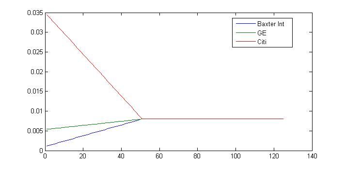
Figure 1: Three rows of the prior matrix $q_{ij}^{(1)}$ corresponding to low, moderate and high spreads.

The ansatz (25) is certainly not the only possible model for the prior. Another method to construct the prior will be presented below after we discuss the single name sensitivities calculation.

3.3 Iterative scaling (IS) algorithm

We assume that an initial guess (a “prior”) $q_{ij}\equiv p_{ij}^{(0)}$ for the solution is available using e.g. a construction just presented (see below for an alternative choice). We then use the iterative scaling algorithm to find the matrix $p_{ij}$. With this method, the matrix is updated iteratively $p^{(0)}\rightarrow p^{(1)}\cdots\rightarrow p^{(k)}\rightarrow p^{(k+1)}\cdots$ according to the following scheme:

$$p_{ij}^{(k+1)}=\left\{\begin{array}[]{ll}p_{ij}^{(k)}\frac{Q_{i}}{\sum_{j}p_{ij}^{(k)}w_{j}}&\mbox{for $k$ odd}\\ \frac{p_{ij}^{(k)}}{\sum_{i}p_{ij}^{(k)}}&\mbox{for $k$ even.}\end{array}\right.$$ (28)

In other words, we alternatively rescale the matrix to enforce the row and column constraints until convergence. The equivalent scheme for joint TD-matrices $P_{ij}$ reads

$$P_{ij}^{(k+1)}=\left\{\begin{array}[]{ll}P_{ij}^{(k)}\frac{Q_{i}}{\sum_{j}P_{ij}^{(k)}}&\mbox{for $k$ odd}\\ P_{ij}^{(k)}\frac{w_{j}}{\sum_{i}P_{ij}^{(k)}}&\mbox{for $k$ even.}\end{array}\right.$$ (31)

We have tested the above algorithm on several datasets, and found in each case fast convergence (in less then 10 steps per maturity) to parameters matching single name CDS spreads with relative errors below 1%. The whole calculation takes about 2-3 seconds on a standard PC. An example of calibrated conditional thinning matrices is given in Fig. 2 for CDX IG8 data on 03/03/2008 (the same dataset will be used for all numerical examples in what follows). Tail probabilities needed for this calculation are produced by our own version of a top-down model called BSLP (Bivariate Spread-Loss Portfolio) model [10], however any other top-down model can be used to this end. Tail probabilities produced by BSLP by calibrating to the same dataset are shown in Fig. 3.

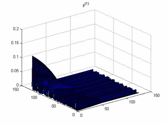
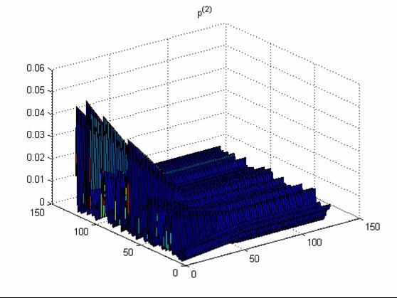
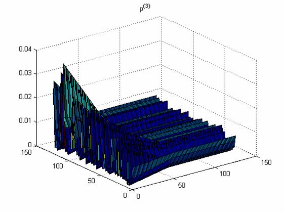
Figure 2: Calibrated thinning matrices $p_{ij}^{(1)},p_{ij}^{(2)},p_{ij}^{(3)}$ for intervals $[0,3Y],\,[3Y,5Y],\,[5Y,7Y]$ for CDX IG8 data on 03/03/2008, obtained with linear prior (25). (The fourth matrix is similar and is not shown here to save space.)

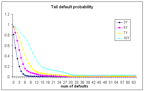
Figure 3: Tail probabilities for horizons of 3,5,7 and 10Y for CDX IG8 data on 03/03/2008 calculated with the BSLP model.

3.4 Information-theoretic interpretation of IS algorithm

If we rescale our matrices $p_{ij}\rightarrow Np_{ij}$ and $q_{ij}\rightarrow Nq_{ij}$ so that now $\sum_{i,j}p_{ij}=\sum_{i,j}q_{ij}=1$, then $\{p_{ij}\},\{q_{ij}\}$ can be thought of as two-dimensional probability distributions. As was shown by Ireland and Kullback [11] and Csiszár [12] (see also [13]), the IS algorithm can be interpreted as an alternative minimization of the Kullback-Leibler divergence (relative entropy, see e.g. [14]) between these two measures:

$$D[p||q]=\sum_{ij}p_{ij}\log\frac{p_{ij}}{q_{ij}},$$ (32)

subject to constraints $\sum_{j=1}^{N}p_{ij}w_{j}=\frac{1}{N}Q_{i}$ and $\sum_{i=1}^{N}p_{ij}=1/N$. The standard approach to this problem uses the method of Lagrange multipliers to enforce the constraints, leading to the following Lagrangian function

$$\mathcal{L}=D[p||q]-\sum_{j}\lambda_{j}\left(\sum_{i}p_{ij}-\frac{1}{N}\right)-\sum_{i}\xi_{i}\left(\sum_{j}p_{ij}w_{j}-\frac{Q_{i}}{N}\right),$$ (33)

which can be solved using convex duality [14], with dimensionality of the problem being the number of Lagrange multipliers $\xi_{i}$, i.e. equal to the number of constraints. The approach of Ireland and Kullback and Csiszár uses instead an alternative recursive minimization of the KL distance (32) where we alternate between enforcing the row constraints only at odd steps, and column constraints only at even steps. This can be shown to precisely correspond to the alternating rescaling of the IS algorithm. This method may be computationally less expensive than the direct minimization of (33), especially for large scale problems, and it allows one to prove convergence of the IS algorithm under certain technical conditions.

We note that the information-theoretic reformulation of the problem can be easily generalized to the case when one matches single name spreads approximately (e.g. in the least square sense) rather than exactly, and thus can be used to ensure stability of single name calibration. We will not pursue this approach further in this paper.

4 Single name sensitivities

The TD-matrices calibrated as of today can be used for calculation of single name sensitivities, as proposed by Giesecke and co-authors [3, 4, 6]. Specifically, once a calibrated set of TD-matrices is found, sensitivity to a given name $i$ is calculated as follows. First we re-scale the $i$-th row in the unconditional TD-matrix to accommodate the new (bumped) spread of the $i$-th name. Once this is done, summation of the new perturbed matrix over $i$ produces a new set of bumped tail probabilities, which is equivalent to bumping tranche prices. The ratio of changes of the MTM of a given tranche to that of the underlying names is the name delta of the tranche.

Let us consider the calculation in more details, focusing for simplicity on the first maturity interval $[0,T_{1}]$. Assume that we want to calculate sensitivity of tranche prices to a given name $i$. To this end, we tweak only the $i$-th row of the joint TD matrix $P_{ij}=P_{ij}^{(1)}$. We consider the simplest proportional tweak of all elements in the $i$-th row:

$$\delta P_{ij}=\varepsilon P_{ij}.$$ (34)

Using Eqs.(2), we obtain the following tweaks of the default probability $Q_{i}(T)$ and tail probabilities $w_{j}$:

$$\delta Q_{i} = \sum_{j=1}^{N}\delta P_{ij}=\varepsilon\sum_{j=1}^{N}P_{ij}=\varepsilon Q_{i},$$

$$\delta w_{j} = \delta P_{ij}=\varepsilon P_{ij}.$$ (35)

Note that as long as the rule (34) of tweak of $P_{ij}$ is specified, the tweak of the conditional TD-matrix $p_{ij}$ is not arbitrary but is rather fixed by the relation

$$\delta P_{ij}=w_{j}\delta p_{ij}+p_{ij}\delta w_{j}.$$ (36)

Substituting (34) and the second of Eqs.(4) and re-arranging, this yields

$$\delta p_{ij}=\varepsilon p_{ij}\left(1-p_{ij}\right).$$ (37)

Eqs.(4) express the sought-after “duality” between tweaks of single name default probability and the tail probability, which both stem from a tweak of the joint TD-matrix $P_{ij}$. It is exactly this duality that enables the whole calculation of single name sensitivities in our framework. What remains now for calculation of those single name sensitivities is to establish a relation between changes of the market-to-market of name $i$ and a tranche with changes $\delta Q_{i}$ and $\delta w_{j}$, respectively.

In what follows, we establish approximate, rather than “exact”, relations for single name sensitivities. Generalizations of formulae to follow to make them “exact” (i.e. include contributions of all cashflows) are straightforward, but lead to bulky expressions and hence will be omitted here. Furthermore, as will be shown later on, our approximate formulas can be inverted, leading to some interesting insights (see Sect. 4.1).

We start with establishing relevant formulae for name $i$. Let us approximate a change of MTM, $\delta MTM_{i}$, of CDS referencing the $i$-th name by a change $\delta DL_{i}$ of its default leg. (Note that this approximation becomes exact if the CDS premium is paid upfront rather than as a running spread. Corrections to this approximation will be considered below.) In turn, $\delta DL_{i}$ can be approximated by the (discounted) change in the expected loss on this name (i.e. the default probability times $(1-R)/N$, assuming a unit portfolio notional). This yields

$$\delta MTM_{i}\simeq\frac{1-R}{N}B(0,T)\delta Q_{i}(T),$$ (38)

where $B(0,T)$ is a discount factor to time $T$.

We can now use the same approximation as above for the MTM change of the tranche, so that the latter is approximated by the (discounted) change of the tranche expected loss (EL). We assume an ordered set of strikes $K_{1},\ldots,K_{N_{tr}}$ expressed as a fraction of the total portfolio notional, with $K_{0}=0$ and $K_{N_{tr}}=1$. Let $EL_{k}\equiv EL_{[K_{k-1},K_{k}]}$ (where $k=1,\ldots,N_{tr}$) be the expected loss of the $k$-th tranche, expressed as a percentage of the tranche notional, is defined as follows (here $I=\frac{1}{N}$ is the CDS notional):

$$EL_{k}=\frac{S_{k-1}-S_{k}}{K_{k}-K_{k-1}},$$ (39)

where

$$S_{k}=\sum_{n=1}^{N}\left((1-R)nI-K_{k}NI\right)^{+}\rho_{n},$$ (40)

and $\rho_{n}$ is the probability of having $n$ defaults by a given time horizon, which can be expressed in terms of the tail probabilities $\{w_{n}\}$ defined in Sect.2:

$$\rho_{n}=\left\{\begin{array}[]{ll}w_{n}-w_{n+1}&\mbox{$n=1,\ldots,N-1$}\\ w_{N}&\mbox{$n=N$.}\end{array}\right.$$ (43)

After some algebra, we obtain for $S_{k}$

$$S_{k}=\frac{1-R}{N}1_{(\hat{K}_{k}<1)}\left(\sum_{\lfloor\hat{K}_{k}N\rfloor}^{N}w_{n}+\left(\lfloor\hat{K}_{k}N\rfloor-\hat{K}_{k}N\right)w_{\lfloor\hat{K}_{k}N\rfloor}\right)\simeq\frac{1-R}{N}1_{(\hat{K}_{k}<1)}\sum_{n=\lfloor\hat{K}N\rfloor}^{N}w_{n},$$

where $\hat{K}_{k}\equiv K_{k}/(1-R)$ and $\lfloor x\rfloor$ stands for the smallest integer equal or larger than $x$. For the tranche expected loss with $\hat{K}_{k-1},\hat{K}_{k}<1$ we therefore have

$$EL_{k}\simeq\frac{1-R}{K_{k}-K_{k-1}}\frac{1}{N}\sum_{n=\lfloor\hat{K}_{k-1}N\rfloor}^{\lfloor\hat{K}_{k}N\rfloor}w_{n}.$$ (44)

Using (44), (38) and (4), we arrive at the following approximate formula for the single name delta of the $k$-th tranche in the random thinning framework:

$$\Delta_{i}^{k} \equiv \frac{(\delta MTM)_{tranche}^{k}}{(\delta MTM)_{i}}\simeq\frac{1}{K_{k}-K_{k-1}}\frac{1}{N}\frac{\sum_{n=\lfloor\hat{K}_{k-1}N\rfloor}^{\lfloor\hat{K}_{k}N\rfloor}\delta P_{in}}{\sum_{n=1}^{N}\delta P_{in}}$$ (45)

$$= \frac{1}{K_{k}-K_{k-1}}\frac{1}{N}\frac{\sum_{n=\lfloor\hat{K}_{k-1}N\rfloor}^{\lfloor\hat{K}_{k}N\rfloor}w_{n}p_{in}}{\sum_{n=1}^{N}w_{n}p_{in}}.$$

Note that this formula readily demonstrates that tweaks $\delta P_{in}=\varepsilon w_{n}p_{in}$ should be different for different names, as otherwise our approximation would produce the same deltas for all names.

We can also calculate the index delta from all single name deltas as follows. If we tweak all single names at once using a proportional tweak with the same $\varepsilon$ for all names, then the change of tranche MTM is

$$(\delta MTM)_{tranche}^{k}=\sum_{i}\Delta_{i}^{k}(\delta MTM)_{i},$$ (46)

while on the other hand by definition it is equal to

$$(\delta MTM)_{tranche}^{k}=\Delta_{idx}^{k}(\delta MTM)_{idx}.$$ (47)

Comparing these two formulas and taking into account the relation

$$(\delta MTM)_{idx}=\sum_{i}\frac{1}{N}(\delta MTM)_{i}=\varepsilon(1-R)B(0,T)\sum_{i=1}^{N}\sum_{n=1}^{N}w_{n}p_{in},$$ (48)

we obtain two relations for the index delta. The first one is a “bottom-up” formula expressing the index delta as a weighted average of single name deltas:

$$\Delta_{idx}^{k}=N\frac{\sum_{i=1}^{N}\Delta_{i}^{k}(\delta MTM)_{i}}{\sum_{i=1}^{N}(\delta MTM)_{i}},$$ (49)

and the second one is a “top-down” relation

$$\Delta_{idx}^{k}=\frac{(\delta MTM)_{tranche}^{k}}{(\delta MTM)_{idx}}\simeq\frac{1}{K_{k}-K_{k-1}}\frac{\sum_{i=1}^{N}\sum_{n=\lfloor\hat{K}_{k-1}N\rfloor}^{\lfloor\hat{K}_{k}N\rfloor}w_{n}p_{in}}{\sum_{i=1}^{N}\sum_{n=1}^{N}w_{n}p_{in}}.$$ (50)

Note that approximate deltas calculated according to (50), and rescaled by the tranche widths $K_{k}-K_{k-1}$, sum up to 1 across all tranches in the capital structure, while single name deltas sum up to $1/N$. Also note the following simple relation between the index delta and single name deltas:

$$\Delta_{idx}^{k}\simeq\sum_{i}\Delta_{i}^{k},$$ (51)

which follows from (49) as long as all spreads in the index portfolio are approximately equal and tweaked in the same way (i.e. using the same value of $\varepsilon$).

We would like to note that the accuracy of approximate formulas (45) and (51) can be improved without adding complexity. This is done by assuming a continuous coupon, and approximating the premium legs of a CDS and a tranche using the a constant riskless rate $r$ and a constant hazard rate $h_{i}$ so that the survival probability of name $i$ reads

$$Q_{i}(T)=e^{-h_{i}T}.$$ (52)

and a similar formula for the survival probability of a tranche. This yields the following value for the premium leg of a tranche

$$PL_{[K_{d},K_{u}]} = s\int_{0}^{T}dte^{-rt}e^{-ht}=\frac{1}{r+h}\left(1-e^{-(r+h)T}\right)\simeq sT\left(1-\frac{1}{2}T(r+h)\right)$$ (53)

$$\simeq sT\left(1-\frac{1}{2}rT-\frac{1}{2}EL_{[K_{d},K_{u}]}\right),$$

where $h$ is the continuous coupon rate. This produces the following refinement to the approximate relation (45):

$$\Delta_{i}^{k}\simeq\frac{1}{K_{k}-K_{k-1}}\frac{1}{N}\frac{B(0,T)+\frac{1}{2}s_{tr}^{k}T}{B(0,T)+\frac{1}{2}s_{i}T}\frac{\sum_{n=\lfloor\hat{K}_{k-1}N\rfloor}^{\lfloor\hat{K}_{k}N\rfloor}w_{n}p_{in}}{\sum_{n=1}^{N}w_{n}p_{in}}.$$ (54)

Numerical experiments indicate that accuracy of the approximate formula (54) in comparison with an “exact” expression that includes contributions of all cashflows is not worse than 10%.

The results of single name sensitivities calculated using (54) are given in Tables  1,  2 and  3 for three names representing low, moderate and high spread names, respectively.

Tranche	0-3%	3-7%	7-10%	10-15%	15-30%	30-100%
BC delta	0.0546	0.0086	-0.0022	-0.0034	-0.0093	0.0109
RT delta (prior 1)	0.0521	0.0218	0.0152	0.0102	0.0085	0.0057
RT delta (prior 2)	0.0283	0.0035	0.0011	0.0005	0.0009	0.0101

Table 1: Single name sensitivities for a low spread name (Baxter).

Tranche	0-3%	3-7%	7-10%	10-15%	15-30%	30-100%
BC delta	0.0900	0.0314	0.0153	0.0136	0.0172	0.0006
RT delta (prior 1)	0.1180	0.0334	0.0175	0.0097	0.0056	0.0034
RT delta (prior 2)	0.1025	0.0345	0.0212	0.0159	0.0156	0.0014

Table 2: Single name sensitivities for a medium spread name (GE).

Tranche	0-3%	3-7%	7-10%	10-15%	15-30%	30-100%
BC delta	0.1914	0.0487	0.0116	0.0028	0.0001	-4.75e-10
RT delta (prior 1)	0.1744	0.0433	0.0195	0.0093	0.0032	0.0013
RT delta (prior 2)	0.1725	0.0595	0.0316	0.0144	0.0021	0.0002

Table 3: Single name sensitivities for a high spread name (Sprint).

A few comments are in order here in regard to these numbers. The first row in these tables labeled “BC delta” shows sensitivities calculated with the base correlation method. Negative entries in Table 1 (and 3) clearly show that the base correlation methodology is “wrong” in the sense that for positive asset correlations, all single name sensitivities in a “right” model should be positive, not negative. Nevertheless, in view of the absence of a market-standard alternative to the base correlation methodology, we will keep base correlation sensitivities as a reference point for our RT scheme. The second row (“RT delta (Prior I)” in the tables refers to single name sensitivities calculated with the “linear” prior (25), while the third row gives the RT delta calculated with the base correlation prior which is explained below in Sect. 4.1. One sees that the RT method produces numbers of the same order of magnitude as the base correlation model, with largest differences being for mezzanine and senior tranches.

At this point, a question that could be asked is which set of deltas is the “right” one. Generally, the ultimate answer to this question requires exploring the behavior of the P&L distribution of the hedged position, where hedges are calculated according to the model. While we do not pursue such an analysis in this paper, we note that RT deltas are likely to be “less wrong” than base correlation deltas as they arise from a consistent, arbitrage-free model. For example, unlike the latter, positivity of RT deltas is guaranteed by construction. More on the comparison between RT sensitivities calculated with Prior I and Prior II will be said in Sect. 4.1, after the “base correlation prior (“Prior II”) is introduced.

4.1 “Base correlation” prior

Assume we are given some set of “target” single name sensitivities which we would like to match as closely as possible. These sensitivities can come from any bottom-up model such as CreditMetrics, approximately calibrated to tranche quotes of interest. Using the results of the last section, we can then invert the relation (54) or (45) and construct the $p$-matrices such that these deltas are approximately matched. We then use these $p$-matrices as priors that need to be corrected by the IS algorithm to match the single-name and portfolio data. The new “true” sensitivities are then calculated using the calibrated TD-matrices.

Note that each row in the $p$-matrix has $N$ elements (e.g. N = 125 for CDX.NA.IG and iTraxx portfolios), while for the same portfolios we have only 6 deltas per name. This means that the problem is severely underdetermined. To reduce the number of free parameters, we assume that for each $i$ and $m$, elements of $p_{ij}^{(m)}$ are piecewise-constant between default counts $j$ that correspond to strikes of tranches in the calibration set. Thus, we set $p_{in}=\bar{p}_{i}^{1}$ for $j\in[1,j_{1}]$, $p_{in}=\bar{p}_{i}^{2}$ for $j\in[j_{1}+1,j_{2}]$, etc. Eq. (45) with a proportional tweak $(\delta p)_{in}=\varepsilon p_{in}$ produces the following formula for the delta of the $k$-th tranche with respect to name $i$

$$\Delta_{i}^{k} \simeq \frac{1}{K_{k}-K_{k-1}}\frac{1}{N}\frac{\sum_{n=\lfloor\hat{K}_{k-1}N\rfloor}^{\lfloor\hat{K}_{k}N\rfloor}w_{n}p_{in}}{\sum_{n=1}^{N}w_{n}p_{in}}=\frac{1}{K_{k}-K_{k-1}}\frac{1}{N}\frac{\sum_{n=\lfloor\hat{K}_{k-1}N\rfloor}^{\lfloor\hat{K}_{k}N\rfloor}w_{n}p_{in}}{Q_{i}(T_{1})}$$ (55)

$$= \frac{1}{K_{k}-K_{k-1}}\frac{1}{N}\frac{\bar{p}_{i}^{k}\sum_{n=\lfloor\hat{K}_{k-1}N\rfloor}^{\lfloor\hat{K}_{k}N\rfloor}w_{n}}{Q_{i}(T_{1})}=\frac{1}{K_{k}-K_{k-1}}\frac{1}{N}\frac{\bar{p}_{i}^{k}\bar{w}^{k}}{Q_{i}(T_{1})},$$

where $\bar{w}^{k}\equiv\sum_{n=\lfloor\hat{K}_{k-1}N\rfloor}^{\lfloor\hat{K}_{k}N\rfloor}w_{n}$. Inverting this relation, we obtain

$$\bar{p}_{i}^{k}=\Delta_{i}^{k}Q_{i}(T_{1})\frac{N(K_{k}-K_{k-1})}{\bar{w}^{k}}.$$ (56)

Similar to Eq. (54), this relation can be improved by taking into account non-vanishing spreads paid by a CDS and a tranche:

$$\bar{p}_{i}^{k}=\Delta_{i}^{k}Q_{i}(T_{1})\frac{N(K_{k}-K_{k-1})}{\bar{w}^{k}}\frac{B(0,T)+\frac{1}{2}s_{i}T}{B(0,T)+\frac{1}{2}s_{tr}^{k}T}.$$ (57)

The result is shown in Fig. 4 for the same three names that were used for illustration of our “linear” prior matrices.

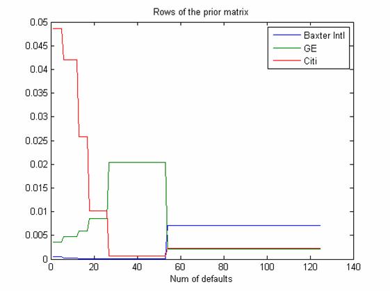
Figure 4: Three rows of the prior matrix $q_{ij}^{(1)}$ corresponding to low, moderate and high spreads, with the “base correlation” prior.

Resulting calibrated thinning matrices are shown in Fig. 5. They can be compared with the profiles displayed in Fig. 4. One sees that the direction behavior is similar in both cases.

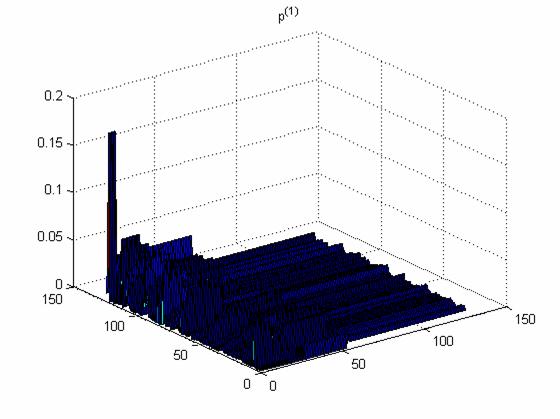
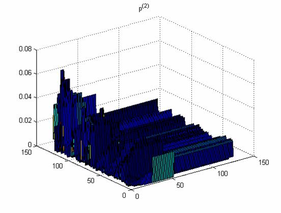
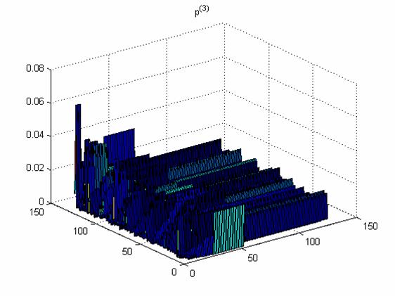
Figure 5: Calibrated thinning matrices $p_{ij}^{(1)},p_{ij}^{(2)},p_{ij}^{(3)}$ obtained with the “base correlation prior”.

Going back to comparison of sensitivity parameters obtained with different RT schemes (see Tables  1-3), the numbers shown there for three selected names do not really demonstrate that sensitivities obtained with the “base correlation prior” are considerably closer to base correlation sensitivities than those obtained with the linear prior. That this is indeed the case is illustrated in Fig. 6 where we show the relative difference between the RT and BC equity delta across different names in the portfolio for both the “linear” and “base correlation” choice for the prior. What can be clearly seen though is that with the first prior our equity delta is generally higher than the BC delta, while with “base correlation” prior the situation is reversed.

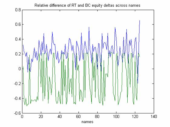
Figure 6: Relative difference of equity delta obtained with the random thinning (RT) and base correlation (BC) method, for the “linear” and “base correlation” choice of the prior.

Thus, our numerical experiment shows that the idea of having a sort of “calibration” of TD matrices to base correlation deltas does not really work, as the the subsequent rescaling of TD matrices (needed to match single name and portfolio data) substantially alternates the prior matrices. While we are not aware of any compelling financial explanation of this behavior, perhaps a more interesting practical conclusion that can be drawn from our experiments with different priors is that single name deltas are not unique, and depend on fine details of the model (in our case, the choice of the prior). As will be further discussed in the concluding section, this situation is in fact quite common, and occurs not only in top-down but in bottom-up models as well.

5 From statics to dynamics: filtering approach

To get the single name dynamics, we need to update the TD-matrices dynamically based on observed information. Updating of TD-matrices is done in two ways: by zeroing out rows and columns corresponding to “observed” (simulated) defaults, and by random perturbation (done in a particular way, see below) of non-zero elements, to account for single name spread volatility. Recall that if our TD-matrices are to be used for pricing today, they must be updated in a fair way: in other words, they must be martingales.

In this section, we consider a particular framework for modeling the filtration $\mathcal{F}_{t}$. Recall from Sect. 2.1, the filtration $\mathcal{F}_{t}$ can be obtained by taking a combination of the natural top-down model filtration (i.e. default times and losses upon defaults, but not defaulters’ identities), the history of defaulters’ identities (obtained by simulation, see below), and the filtration generated by observation of “information processes” (see below) for all names. These three components of the filtration $\mathcal{F}_{t}$ will be used below update the TD-matrices based on portfolio losses, and the “information process” dynamics.

5.1 Default history filtration

In this section we consider updating our TD-matrices based on defaults in the portfolio, i.e. adaptation of TD-matrices to the natural filtration of a top-down model. This is the most basic form of updating, and is necessary for simulation of defaulters’ identities. We assume for now that there is no updating based on “information processes” (see the next section) and so in the notation of Sect.2.1, the filtration $\mathcal{F}_{t}$ is generated purely by the history of the portfolio-level default counting process, $(\mathcal{G}_{t})_{t\geq 0}$, and the identities of the defaulters, $(\mathcal{I}_{t})_{t\geq 0}$. In this section we replace the time dependence of the TD-matrices (representing the fact that we condition of $\mathcal{F}_{t}$) by a dependence on the number of defaults up to time $t$, $k\in\{0,1,2,\ldots,N\}$.

We assume that the initial portfolio contains no defaulted names. Let us denote the calibrated conditional $TD$-matrices as $p_{ij}^{(m)}(k=0)$. Assume we simulate the portfolio dynamics using Monte Carlo, and the first default in the portfolio happens at time $\tau^{1}$. Conditional on the fact that a default has occurred, we independently simulate the identity of the defaulter with probabilities that depend on the relation between $\tau^{1}$ and the reference maturities $T^{(m)}$. Let us first assume that $\tau^{1}<T^{(1)}$. In this case, we simulate the identity $I_{1}\in\{1,2,\ldots,N\}$ of the first defaulter according to the conditional distribution $\{p_{i1}^{(1)}(k=0),i=1,\ldots,N\}$:

$$P(I_{1}=i|\tau^{1}<T^{(1)})=p_{i1}^{(1)}(k=0).$$ (58)

Note that we have some freedom here: instead of simulating from conditional probabilities as determined by the TD-matrices at time 0, we may alternatively simulate from TD-matrices that have been dynamically updated as described in the next section to the time of actual default. In the case when the first default happens in the interval $[T^{(m-1)},\,T^{(m)}]$ with $m>1$, we have:

$$P(I_{1}=i|T^{(m-1)}\leq\tau^{1}<T^{m})=p_{i1}^{(m)}(k=0).$$ (59)

Note that the method in (58) (or (59)) is similar to that used previously by Duffie [9] (in the context of a bottom-up approach) to probabilistically pick a defaulter identity in a first-to-default basket where the simulated process is the aggregate portfolio default intensity. Unlike Duffie who employs a one-period setting, in our framework the conditional probabilities $p_{i}^{(m)}$ are adapted to the model filtration in a dynamic way.

Conditional on the fact of “observing” (for this particular Monte Carlo scenario) default of name $I_{1}$, we now want to update our p-matrices $p_{ij}^{(m)}(k=0)\rightarrow p_{ij}^{(m)}(k=1)$. In other words, we want to calculate conditional probabilities

$$p_{ij}^{(m)}(k=1)=P\left[\tau^{j}=\tau_{i}|T^{(m-1)}\leq\tau_{i}\leq T^{(m)},I_{1},\tau^{1}\right]\,,\;j=2,\ldots,N,\,i=1,\ldots,N.$$ (60)

We use the simplest possible “model” for these conditional probabilities:

$$p_{ij}^{(m)}(k=1)=\left\{\begin{array}[]{lll}P\left[\tau^{j}=\tau_{i}|T^{(m-1)}\leq\tau_{i}\leq T^{(m)},\tau^{1}\right]&\mbox{if $i\neq I_{1}$}\\ 0&\mbox{if $i=I_{1}$}.\end{array}\right.$$ (63)

In words, we assume that all rows with $i\neq I_{1}$ in the updated P-matrix do not depend on the identity of the first defaulter for all $j\geq 2$, while the row with $i=I_{1}$ is zeroed out. Note that our choice is related to the fact that the natural filtration of the top-down model only contains default times but not identities of defaulters. Therefore, anything more complicated than (63) would amount to some sort of a bottom-up, rather than top-down, approach.

What remains now is to come up with a method to calculate the conditional probabilities in (63). Again, note that we aim at a simplest possible dynamic model consistent with the portfolio-level dynamics of the top-down model and its natural filtration. To this end, we note that the new updated probabilities should still satisfy the first of constraints (2), where the new right hand side can now be calculated for all $j\geq 2$ using the top-down model. Respectively, we obtain a simplest model for (63) by a uniform rescaling of all probabilities $p_{ij}^{(m)}(k=0)$ for all $j\geq 2$ and $i\neq I_{1}$ so that the first constraint in (2.2) is re-enforced:

$$p_{ij}^{(m)}(k=1)=\frac{p_{ij}^{(m)}(k=0)}{1-p_{I_{1}j}^{(m)}(k=0)}\;,\;\;i\neq I_{1},\;j=2,\ldots,N.$$ (64)

Note that after this rescaling is done, we get different marginal forward default probabilities $P\left[\left.T^{(m-1)}\leq\tau_{i}\leq T^{(m)}\right|\mathcal{F}_{t}\right]$ for surviving names, which are obtained if we sum the product of the new conditional probabilities $p_{ij}^{(m)}(k=1)$ with the newly calculated tail probabilities over $j$. Extending the above analysis to the second, third, etc. defaults, we have the following scheme for simulation of defaulters’ identities and updating the conditional p-matrices. For each sequential default, we simulate the defaulter’s identity from the current p-matrices, as in (58), and then zero out the corresponding column and row in the current p-matrices. We then rescale the current p-matrices so that the column-constraints are satisfied. The new re-scaled p-matrices are used in conjunction with the tail probabilities $w_{k}^{(m)}(j)$ to calculate the new forward marginal default probabilities for surviving names.

Qualitatively, the impact of defaults on default intensities of surviving names can be described as an interplay between three effects. To explain them, consider a particular scenario where we observed $n$-th default at time $t$. Assuming the identity of this defaulter is $I_{t}$, we zero out the $I_{t}$-th row in all forward matrices, and rescale all columns of $p_{ij}$ for all $j>n$ to re-establish the column constraints. This has an effect of bumping all probabilities $p_{ij}$ for any fixed $j>n$. However, we have also to take into account the fact that when a default occurs, the “next-to-default” column in the $p$-matrices moves one step to the right. Therefore, the impact of this default on short-term spreads of surviving names will be determined by a combined effect of three factors: 1) we move one column to the right in the $p-$ (or $P-$) matrices, 2) we rescale this column to re-enforce the column constraint, and 3) we multiply the result by the new portfolio-level intensity $\lambda_{n}$ corresponding to $n$ defaults in the portfolio, instead of a previous multiplication by $\lambda_{n-1}$. As $\lambda_{n}$ is generally an increasing function of $n$, the net effect will be largely driven by the first two factors. This implies, in particular, that for the simple model with a “uniformization bound” for names with low spread we will have a relation $p_{i,j+1}>p_{ij}$, so the net effect will be to increase the default intensity. For names with high initial spreads, we have an inverse relation $p_{i,j+1}<p_{ij}$, and therefore the resulting change of their default intensity can be of any sign, depending on the relative strength of two effects. This is largely consistent with what is observed in the markets: upon defaults, low-spread names (especially those in the same industry/sector) are expected to go up due to informational contagion, while high spread names do not necessarily widen - they may already be wide enough to start with.

Examples of default updating of low spread and high spread names for a scenario with three defaults happening at 2, 4 and 6 years are displayed in Figs. 7 and 8 where we show updating of a single row in conditional TD-matrices upon portfolio defaults for low- and high-spread names, respectively. The resulting jumps in single name intensities (as expected, more pronounced for a low spread name) manifest the credit contagion at the single name level.

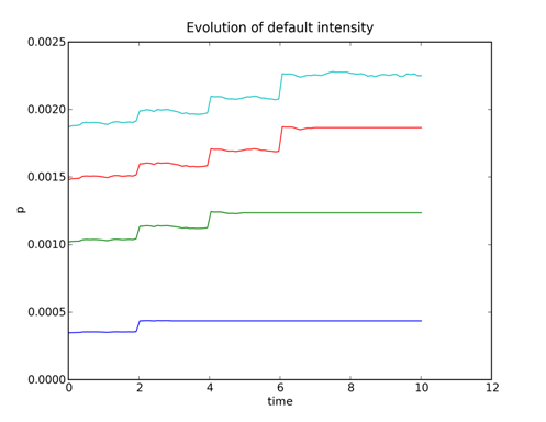
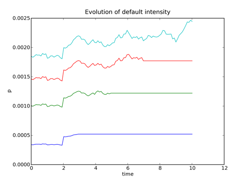
Figure 7: Default updating of conditional TD-matrices: a row corresponding to a low spread names for matrices $p_{ij}^{(m)}$ for all maturity intervals $m=1,2,3,4$. (Note that each line flattens out at the end of its maturity interval. The lowest and top-most lines correspond to $m=1$ and $m=4$, respectively.) The two graphs correspond to regimes of low and high volatility of background “information” process. One sees that adding volatility does not completely wash out jumps resulting from the default updating.

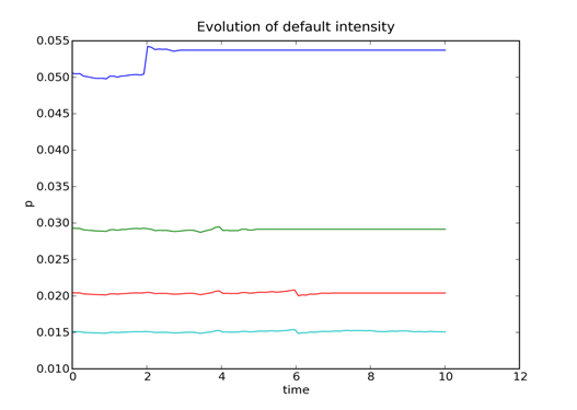
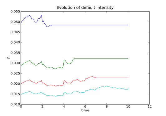
Figure 8: Default updating of conditional TD-matrices: a row corresponding to a high spread names. (Note that ordering of lines is reversed in comparison to Fig. 7: the top-most line corresponds to $m=1$, and the line at the bottom corresponds to $m=4$.) The two graphs correspond to regimes of low and high volatility of background “information” process. One sees that the only clearly seen jump occurring for matrix $p^{(1)}_{ij}$ is washed out when volatility is added.

5.2 Spread dynamics

Applying the default updating procedure above leads to matrices $p_{ij}^{(m)}$ that are piecewise constant between defaults. From Sect.2, this implies that the forward default probabilities of the single names are perfectly correlated with the index, which is unrealistic. In order to remedy this, we must condition on additional information; in addition to observing defaults and the identities of defaulting names, we now assume that for each name $i$, we observe an “information process” $X_{i}$ driven by a Brownian motion. The filtration $(\mathcal{H}_{t})_{t\geq 0}$ introduced in Sect. 2.1 is assumed to be generated by the joint history of the information processes $\{X_{i}\}$ for all names. We note that the processes $\{X_{i}\}$ may be correlated with each other, and for each name $i$, its process $X_{i}$ can be correlated with market observables such as the equity price. While many functional forms for $X_{i}$ are possible (e.g. $X_{i}$ could be a GBM or OU process), we restrict ourselves below to a simplest case of a Brownian diffusion with an unknown random drift.

To model stochasticity in the TD-matrices, we assume that information about the order of defaulting names (first to default, etc) is encoded in the drifts of the $X_{i}$’s, while the accuracy of our information about the $i$-th name is described by the volatility of the $X_{i}$. For simplicity, we concentrate on modeling stochasticity of the next-to-default intensities (i.e. the nearest “active” columns $p_{i}^{m}(t)\equiv p_{ik}^{(m)}(t)$ (with $i=1,\ldots,N$) of the conditional TD-matrices in a scenario where we have $(k-1)$ previous defaults).

We assume that for a given Monte Carlo scenario, some names have already defaulted by a previous time $s<t$, and that $p_{i}^{m}(s)$ was already adapted to filtration $\mathcal{F}_{s}$.

Let $\bf{X}_{t}$ be an $n$-dimensional Itô process described by the following stochastic differential equation (SDE):

$$d{\bf X}_{t}={\bf{\Theta}}_{t}dt+\Gamma d\bf{W}_{t},$$ (65)

where the volatility matrix $\Gamma$, with elements $\Gamma_{ij}=\sigma_{ij}$, satisfies the constraints

$$\left(\Gamma\Gamma^{\prime}\right)_{ij}=\Sigma_{ij}=\rho_{ij}\sigma_{i}\sigma_{j},$$ (66)

(here $\Sigma$ stands for the covariance matrix), and the $n$-dimensional drift ${\bf{\Theta}}_{t}$ follows a $N$-state continuous time Markov chain over states $\{{\bf{\Theta}}_{1},{\bf{\Theta}}_{2},\ldots,{\bf{\Theta}}_{N}\}$ with generator matrix $\Lambda$. In our case, we set $n=N$, i.e. the dimension of the information process is equal to the size of the portfolio. We will, however, keep using different symbols $N$ and $n$ in the formulas below in order to clarify whether we operate on hidden $(N)$ or observable $(n)$ degrees of freedom. The unobservable vector-valued drift $\bf{\Theta}_{t}$ with values

$${\bf{\Theta}}_{i}=\left(\begin{array}[]{clcr}\Theta_{i1}\\ \Theta_{i2}\\ \vdots\\ \Theta_{in}\end{array}\right)=\left(\begin{array}[]{clcr}\delta_{i1}\\ \delta_{i2}\\ \vdots\\ \delta_{in}\end{array}\right)\;,\;\;i=1,\ldots,N,$$ (75)

describes the identity of the next defaulter: if name 1 is to default next, then ${\bf{\Theta}}={\bf{\Theta}}_{1}=(1,0,\ldots,0)^{\prime}$, if name 2 is the next defaulter, then ${\bf{\Theta}}={\bf{\Theta}}_{2}=(0,1,\ldots,0)^{\prime}$, etc.

We assume that the market filtration $\mathcal{F}_{t}$ is generated by continuous observation of the process $\bf{X}$. We are therefore faced with the problem of inference on a hidden state ${\bf\Theta}_{t}$ given the observation of $\bf{X}$. In other words, we want to calculate the posterior probability

$$\pi_{i}(t)=P\left[\bf{\Theta}_{t}=\bf{\Theta}_{i}|\mathcal{F}_{t}\right],$$ (76)

given the prior probabilities

$$\pi_{i}(0)=\hat{\pi}_{i}.$$ (77)

5.2.1 Continuous time formulation

As shown by Liptser and Shiryaev [15], the posteriors (76) satisfy the following system of stochastic differential equations:

$$d\pi_{i}(t)=\sum_{j=1}^{N}\pi_{j}(t)\lambda_{ji}dt+\pi_{i}(t)\hat{\Gamma}_{i}d\tilde{\bf{W}_{t}}.$$ (78)

Here $\hat{\Gamma}_{i}=\left(\hat{\Gamma}_{i1},\ldots,\hat{\Gamma}_{in}\right)$ with elements

$$\hat{\Gamma}_{ij}=\frac{\Theta_{ij}-\bar{\bf{\Theta}}_{j}}{\sqrt{\sum_{m=1}^{n}\sigma_{jm}^{2}}}=\frac{\delta_{ij}-\bar{\bf{\Theta}}_{j}}{\sigma_{j}},$$ (79)

is the matrix of volatilities of beliefs,

$$\bar{\bf{\Theta}}=\left(\begin{array}[]{clcr}\bar{\Theta}_{1}\\ \bar{\Theta}_{2}\\ \vdots\\ \bar{\Theta}_{n}\\ \end{array}\right)=\sum_{i=1}{\bf{\Theta}}_{i}\pi_{i}(t)=\sum_{i=1}\pi_{i}(t)\left(\begin{array}[]{clcr}\Theta_{i1}\\ \Theta_{i2}\\ \vdots\\ \Theta_{in}\end{array}\right)=\left(\begin{array}[]{clcr}\pi_{1}\\ \pi_{2}\\ \vdots\\ \pi_{n}\end{array}\right),$$ (92)

is the expected drift, and $\tilde{\bf{W}}_{t}=\left(\tilde{W}_{t}^{1},\ldots,\tilde{W}_{t}^{n}\right)^{\prime}$ is a $\mathcal{F}_{t}$-adapted $n$-dimensional Brownian motion (“innovation process”) with components

$$d\tilde{W}_{t}^{j}=\frac{1}{\sqrt{\sum_{k=1}^{n}\sigma_{jk}^{2}}}\left(dX_{t}^{j}-\bar{\Theta}_{j}dt\right)\;,\;\;j=1,\ldots,n,$$ (93)

that is assumed to be observable by investors. Its covariance is calculated as follows:

$$\langle d\tilde{W}_{t}^{j}d\tilde{W}_{t}^{k}\rangle=\frac{\sum_{n}\sigma_{jn}\sigma_{kn}}{\sqrt{\sum_{n}\sigma_{jn}^{2}\sum_{m}\sigma_{km}^{2}}}\,dt\equiv\frac{\left(\Gamma\Gamma^{\prime}\right)_{jk}}{\sigma_{j}\sigma_{k}}\,dt=\rho_{jk}dt,$$ (94)

where we used (66). The instantaneous lognormal volatility $\hat{\sigma}_{i}$ of $\pi_{i}$ is given by:

$$\hat{\sigma}_{i}^{2}=\sum_{j,k}\hat{\Gamma}_{ij}\hat{\Gamma}_{ij}\frac{\langle d\tilde{W}_{t}^{j}d\tilde{W}_{t}^{k}\rangle}{dt}=\sum_{j,k}\frac{\delta_{ij}-\pi_{j}}{\sigma_{j}}\frac{\delta_{ik}-\pi_{k}}{\sigma_{k}}\rho_{jk}.$$ (95)

In our setting, we take $\Lambda=0$, i.e. we consider the identity of the next defaulter to be a random variable rather than a random process. Eq. (78) in this case reduces to

$$d\pi_{i}(t)=\pi_{i}(t)\hat{\Gamma}_{i}d\tilde{\bf{W}_{t}}.$$ (96)

A few comments on the structure of Eqs.(96) and (78) are in order here. First, we observe that the posterior probabilities $\pi_{i}$ specified by (96) are martingales. Second, both Eqs.(78) and (96) ensure conservation of probability $\sum_{i}d\pi_{i}(t)=0$. Third, we note that the diffusion term in both (78) and (96) vanishes in both limits $\pi_{i}\rightarrow 0$ and $\pi_{i}\rightarrow 1$: the first result holds as the diffusion term is proportional to $\pi_{i}$, and the second results follows by the structure of (95) . Lastly, note that in the limit where $\sigma_{i}\rightarrow\infty$ for all $i$, Eq. (78) reduces to the forward Kolmogorov equation as it should, since in this case, observation of the “information process” is useless for inference of the hidden Markov chain.

5.2.2 Discrete time formulation

In practice, simulation using Eq. (78) or (96) can be somewhat tricky as discretization may lead to spurious negative probabilities, non-conservation of probability, etc, similar (but more involved) to problems arising in discretization of e.g. a CIR process. In this view, it may still be preferable to use a discrete-time formulation based on Bayes’ theorem for simulation, while retaining the SDE formulation for calibration (see below on this).

Let $D_{t}$ be the data that becomes available at time $t$; in our case $D_{t}=\{X_{t}^{i}\}$). Therefore, we use Bayes’ theorem

$$p(I_{next}=i|D_{t},\mathcal{F}_{s})=p(I_{next}=i|\mathcal{F}_{s})\frac{P(D_{t}|I_{next}=i,\mathcal{F}_{s})}{\sum_{i}p(I_{next}=i|\mathcal{F}_{s})P(D_{t}|I_{next}=i,\mathcal{F}_{s})},$$ (97)

to adapt our probabilities to filtration generated by information processes $\{X_{t}^{i}\}$. We thus get the updating rule:

$$p_{i}^{m}(t+\Delta t)=p_{i}^{m}(t)\frac{P\left[\Delta{\bf X}_{t}|{\bf\Theta}_{t}={\bf\Theta}_{i}\right]}{\sum_{i}P\left[\Delta{\bf X}_{t}|{\bf\Theta}_{t}={\bf\Theta}_{i}\right]P\left[{\bf\Theta}_{t}={\bf\Theta}_{i}\right]},$$ (98)

where

$$P\left[\Delta{\bf X}_{t}|{\bf\Theta}_{t}={\bf\Theta}_{i}\right]\sim\exp\left(-\frac{1}{2\Delta t}\left(\Delta{\bf X}_{t}-{\bf\Theta}_{i}\Delta t\right)^{T}\Sigma^{-1}\left(\Delta{\bf X}_{t}-{\bf\Theta}_{i}\Delta t\right)\right).$$ (99)

This can be generated by simulating the defaulter identity $k$ and a standard normal random variable $Z_{t}^{j}$:

$$\Delta{\bf X}_{t}=\Delta t{\bf\Theta}_{k}+\sqrt{\Delta t}{\bf W}.$$ (100)

Simplifying, we obtain

$$p_{i}^{m}(t+\Delta t)=\frac{p_{i}^{m}(t)L_{i}\left(\Delta{\bf X}_{t}\right)}{\sum_{i}p_{i}^{m}(t)L_{i}\left(\Delta{\bf X}_{t}\right)},$$ (101)

where the likelihood $L_{i}$ is given by

$$L_{i}\left(\Delta{\bf X}_{t}\right)=\exp\left[\left(\Sigma^{-1}\Delta{\bf X}_{t}\right)_{i}-\frac{\Delta t}{2}\Sigma^{-1}_{ii}\right].$$ (102)

6 Numerical algorithm

Start by setting $k=1$, where the index $k$ enumerates the number of the next default. Then for $k\geq 1$:

1. Default Simulation ($\tau^{k}$): Given $k\geq 1$, simulate $\tau^{k}$ according to the top-down model, and find the index $m$ of the forward interval such that $\tau^{k}\in[T^{(m-1)},T^{(m)}]$.

2. Identity Simulation ($I_{k}$): Simulate the identity of the $k$th defaulter by sampling from the $k$-th column of the p-matrix for the $m$-th forward interval.

3. Information Updating (on $[\tau^{k-1},\tau^{k}]$, optional): Use information process filtering to update the p-matrices to time $\tau^{k}$. The Bayesian update ensures the dynamics of the p-matrices are consistent with the identity simulation step above.

4. Default Updating (at $\tau^{k}$): This step ensures that future identities are simulated consistently with the identity simulation step above (i.e. no repeat defaulters).

   1. Zero out the $I_{k}$-th row of all p-matrices.

   2. Zero out the $k$-th column of all p-matrices.

   3. Re-enforce column constraints for the p-matrices.

5. Repeat: If $\tau^{k}$ is less than the final maturity, increment $k\rightarrow k+1$ and go to Step 1.

Note that as soon as some $\tau^{k}>T^{m}$, the $m$-th p-matrix can be dropped from any future updating steps, as the simulation has progressed beyond the point at which this matrix applies.

7 Marking parameters of the information updating

As discussed above, volatility and correlation parameters of the information processes impact the volatilities and correlation of the resulting single name spreads. Therefore, one can attempt to mark those parameters in such a way that the model-implied behavior of single name spreads will be roughly consistent with the empirical behavior. In this section we present a semi-quantitative analysis toward this goal. Note that there are a few reasons why we will not discuss an accurate calibration. First, empirical variances and especially covariances are subject to large measurement errors, and ideally should be “noise-undressed” before the use. Second, the relation between vols and correlations of the driving Brownian motions and vols and correlation of observable spreads is highly non-linear and hard to work with unless a number of approximations are made.

In principle, the task of approximate calibration/marking of correlation parameters can be done using two alternative approaches. The first one is to work with probabilities, i.e. conditional forward TD matrices and tail probabilities coming from the top-down model. The second way is to use spot default intensities as proxies for finite maturity spreads, and work with them. We choose the second route as it appears simpler technically.

Consider again formulas (11) and (13), which we repeat here for convenience :

$$\lambda_{t}^{i}=Z_{t}^{i}\lambda_{t}^{p}\;,\;\;\ Z_{t}^{i}=p_{i,N_{t}}^{(1)}1_{(t\leq T_{1})}+p_{i,N_{t}}^{(2)}1_{(T_{1}<t\leq T_{2})}+\ldots$$ (103)

Assume that we want to calibrate volatility structure of Brownian motion in the no-default environment for $t<3Y$. We can then identify the thinning parameters $Z_{t}^{i}$ with the first column $\pi_{i}\equiv p_{i1}^{m}$ of the first ($m=1$) conditional $p$-matrix. From (103) we obtain (omitting the time index and denoting $\lambda_{t}^{p}\equiv\lambda$ to ease the notation)

$$\frac{d\lambda_{i}}{\lambda_{i}}=\frac{\pi_{i}d\lambda+\lambda d\pi_{i}}{\pi_{i}\lambda}=\frac{d\lambda}{\lambda}+\frac{d\pi_{i}}{\pi_{i}},$$ (104)

which yields

$$\langle\frac{d\lambda_{i}}{\lambda_{i}}\,\frac{d\lambda_{k}}{\lambda_{k}}\rangle=\langle\left(\frac{d\lambda}{\lambda}\right)^{2}\rangle+\langle\frac{d\lambda}{\lambda}\,\frac{d\pi_{k}}{\pi_{k}}\rangle+\langle\frac{d\pi_{i}}{\pi_{i}}\,\frac{d\lambda}{\lambda}\rangle+\langle\frac{d\pi_{i}}{\pi_{i}}\,\frac{d\pi_{k}}{\pi_{k}}\rangle.$$ (105)

As we assume independence between the $Y$-process and Brownian motion $\tilde{{\bf W}}_{t}$, the cross terms in this formula vanish, and we obtain

$$C_{ij}^{\pi}dt\equiv\langle\frac{d\pi_{i}}{\pi_{i}}\,\frac{d\pi_{j}}{\pi_{j}}\rangle=\langle\frac{d\lambda_{i}}{\lambda_{i}}\,\frac{d\lambda_{j}}{\lambda_{j}}\rangle-\sigma_{Y}^{2}dt.$$ (106)

Note that this matrix is orthogonal to the vector $\pi$:

$$\sum_{j}C_{ij}^{\pi}\pi_{j}dt=\langle\frac{d\pi_{i}}{\pi_{i}}\sum_{j}d\pi_{i}\rangle dt=0,$$ (107)

because $\sum_{j}d\pi_{j}=0$ according to Eq. (96).

We use (106) as a constraint on the covariance of posterior probabilities $\pi_{i}(t)$ by approximating the first term in the right hand side by the empirical covariance matrix of spread returns (times $dt$). On the other hand, we can calculate the covariance matrix of $d\pi_{i}/\pi_{i}$ using Eq. (96):

$$\langle\frac{d\pi_{i}}{\pi_{i}}\,\frac{d\pi_{k}}{\pi_{k}}\rangle=\sum_{j,l}\hat{\Gamma}_{ij}\hat{\Gamma}_{kl}\langle d\tilde{W}_{t}^{j}\,d\tilde{W}_{t}^{l}\rangle=\left(\hat{\Gamma}\rho\hat{\Gamma}^{\prime}\right)_{ik}dt\equiv\left(\gamma\mathcal{R}\gamma^{\prime}\right)_{ik}dt,$$ (108)

where $\gamma_{ij}=\delta_{ij}-\pi_{j}$ and $\mathcal{R}_{ij}=\frac{\rho_{ij}}{\sigma_{i}\sigma_{j}}$. Note that matrix $\gamma$ is degenerate, therefore we cannot directly invert Eq. (108) to find matrix $\mathcal{R}$ from $C^{\pi}$. However, a solution to this equation can be easily found as long as the orthogonality relation $C\pi=0$ holds. Indeed, in this case we find

$$\gamma C\gamma^{\prime}=\left(1-1\cdot\pi^{\prime}\right)C\left(1-\pi\cdot 1^{\prime}\right)=C,$$ (109)

which shows that $\mathcal{R}=C$ is a solution of (108) as long as $C\pi=0$. Note that in theory, matrix $C$ is indeed orthogonal to $\pi$ as shown in (107). However, in our treatment we approximate matrix $C$ using observable spreads, see again (106). In doing so, the orthogonality property is generally lost, and thus such an estimated matrix $C$ does not solve (108) anymore.

This observation prompts a way of solving Eq. (108) approximately (in the least square sense) rather than exactly. Namely, for a given empirical matrix $C$, we find a matrix $\hat{C}$ such that $\hat{C}$ is as close as possible to $C$ (e.g. in the sense of Frobenius norm), while on the other hand satisfying the orthogonality constraint $\hat{C}\pi=0$. Once such a matrix $\hat{C}$ is found, the approximate solution of (108) is given by $\mathcal{R}=\hat{C}$.

A candidate solution satisfying the orthogonality relation can be presented:

$$\hat{C}_{ij}^{(1)}=C_{ij}-\frac{\left(C\pi\right)_{i}\left(\pi^{\prime}\cdot C\right)_{j}}{\pi^{\prime}C\pi},$$ (110)

however it does not guarantee that matrix $\hat{C}$ defined in this way is the closest possible to $C$. The matrix closest to $C$ is instead given by the usual projector

$$\hat{C}_{ij}^{(2)}=C_{ij}-\frac{\pi_{j}}{||\pi||^{2}}\sum_{k}C_{ik}\pi_{k}.$$ (111)

However, such a matrix $\hat{C}$ cannot be the right solution as it is non-symmetric. We have therefore set up a recursive algorithm where we alternate between the first step that calculates the orthogonal projection (111), and the second step where the resulting matrix is made symmetric and positive definite by truncating (zeroing out) any possible negative eigenvalues. As the second step can be viewed as a projection on a convex set of positive-definite symmetric matrices, our procedure amounts to alternating projections on two convex sets, which is known to converge.

In practice, with our particular dataset that we used to test our method (see below), we found that doing 10 to 20 iteration of such procedure provides a matrix that is approximately orthogonal to $\pi$ with a good accuracy, while being symmetric and positive definite. The Frobenius norm of the difference $||\hat{C}-C||^{2}=\sum_{ij}\left(\hat{C}_{ij}-C_{ij}\right)^{2}$ calculated with this method was found to be about 3 times smaller than the norm of the difference calculated according to (110).

To check accuracy of these approximations and to provide a numerical example, we have analyzed one year of daily tranche and single name data for CDX IG8 ending at 03/03/08. We present our results for averages across all names in the portfolio, rather than individual names. Using (106) for all names and assuming $\sigma_{Y}=0.35$, we find that the portfolio-average volatility of $\{\pi_{i}\}$ is 1.71, with a minimum of 1.33, maximum of 7.68, and the standard deviation (std) of 0.6. The portfolio-average correlation between different $\pi_{i}$’s is 0.58, with std of 0.13. We then use the procedure described above to calibrate the parameters of the Brownian motions. This produces the average volatility of 0.68, with the minimum and maximum of 0.13 and 1.93, respectively, and std 0.08. The mean correlation of Brownian motions is 0.48 and std is 0.28. We then simulate the information updating scheme using these parameters of the Brownian motion, and compute output volatility and correlations of posterior probabilities $\{\pi_{i}\}$.

Results are displayed in Table  4.

numRuns	meanVol	stdVol	meanCor	stdCor
500	$1.63\pm 0.10$	$1.08\pm 0.02$	$0.63\pm 0.02$	$0.34\pm 0.01$
1000	$1.64\pm 0.08$	$1.09\pm 0.01$	$0.62\pm 0.01$	$0.34\pm 0.01$

Table 4: Monte Carlo output volatilities and correlations of posterior probabilities $\{\pi_{i}\}$.

One sees that the agreement between the input and output parameters is reasonable though not exact. Factors that contribute to the mismatch are noise in the data, possible non-stationarity of credit spreads dynamics, and potential loss of accuracy in proxying the covariance matrix of $\pi_{i}$’s by the empirical covariance matrix. Furthermore, we found it necessary to truncate small eigenvalues in the resulting covariance matrix of Brownian motions calculated as described above. The need for this procedure arises because when an unadjusted covariance matrix obtained as described above is used for simulation, in a substantial fraction of Monte Carlo scenarios we find the phenomenon of a “super-fast learning”, where the identity of the next defaulter is learned too fast, so that spread volatilities drop to zero after a short (1-2 years) initial period of high volatility, which is clearly not a desirable behavior. The origin of this behavior can be traced back to Eq.(102) defining the likelihood function: when small eigenvalues are present in the covariance matrix, the likelihood becomes large, and the hidden state is learned almost with certainty. A truncation of small eigenvalues of the covariance matrix makes the process more stationary and thus fixes this problem, albeit perhaps not in a way most attractive from a theoretical standpoint. We would like to note, however, that adding actual defaults to sample paths is able to mitigate the effect of super-fast learning as a name will likely default before filtering will show this name as a sure next defaulter. Therefore, we believe that in practice, incorporating defaults together with a truncation of eigenvalues provides a satisfactory solution to the problem of possible super-fast learning. A few more related comments will be made in the next section.

We show in Fig. 9 sample paths of the short-term default intensity (elements of the next-to-default columns in the conditional TD-matrices) for high- and low-spread names.

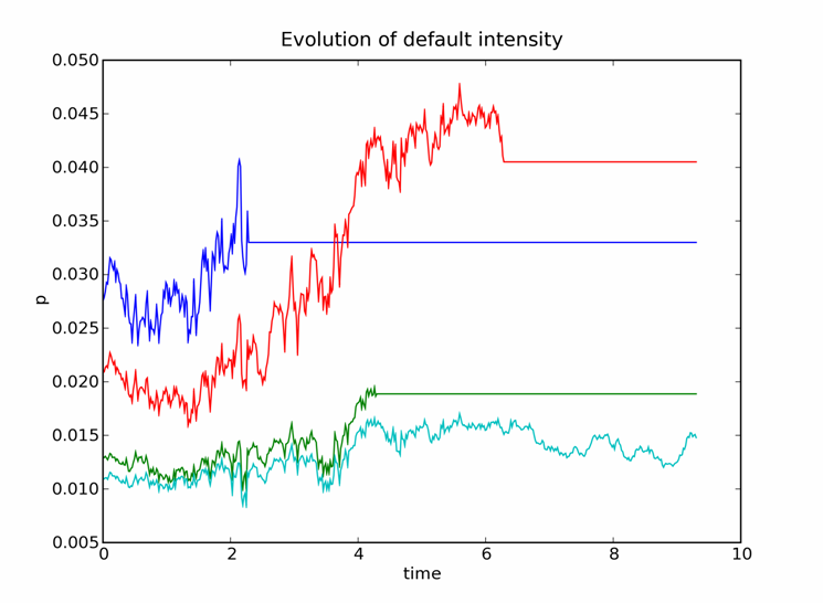
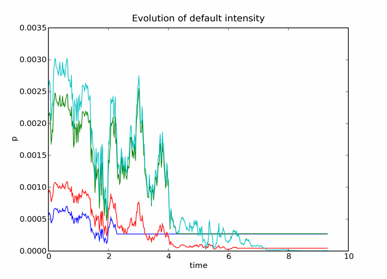
Figure 9: Sample paths for simulated p-matrices with calibrated parameters for high- and low-spread names (the left and right graphs, respectively). These sample paths produce no portfolio defaults. Shown are the next-to-default elements of corresponding rows of matrices $p_{ij}^{(1)}$ to $p_{ij}^{(4)}$.

8 Summary and discussion

In summary, we have presented a practically-oriented random thinning (RT) framework, with an attempt geared toward flexibility, accuracy and numerical efficiency. In particular, our parametrization of TD-matrices is tailored to a very fast (as compared to more traditional inner point methods that would be required with a different parametrization) iterative scaling (IS) method. Furthermore, we have attempted to extend this approach to a dynamic single name setting by developing a scheme for the default and “information process” updating, and have presented a numerical scheme for marking model parameters.

Our proposed dynamic scheme is not free of drawbacks. In particular, we are only able to match CDS spread volatilities and correlations in the portfolio-averaged sense but not on the name-by-name basis. We believe that this still can be considered (modest) progress in the right direction, given the fact that most, if not all, bottom-up models, either struggle in calibrating to these data, or give it up altogether. Better control of volatilities and correlations of spreads in a basket is likely to be important for derivatives that are sensitive to both spread and default dynamics of a credit portfolio.

Another drawback of our approach is a potential “super-fast learning” (see the discussion at the end of last section). The possibility of a super-fast learning stems from a combination of high volatilities of credit spreads (i.e. the current market environment), and the fact that we learn a fixed, albeit unknown, hidden state, i.e. a random variable, not a random process. We have found a way to semi-empirically tackle this issue by truncating small eigenvalues of the Brownian covariance matrix, however a more principled approach would be clearly desirable. A possibility of changing the scheme so that a hidden process, rather than a hidden state would be learned, in a way that respects no-arbitrage martingale constraints, is currently an open question.

In conclusion, we would like to discuss a few further issues that are related to the model presented here.

8.1 Valuing bespoke tranches

The problem of pricing and risk management of bespoke tranches off liquid index tranches is of acute interests for practitioners. The current industry-standard methods typically involve some form of mapping base correlations for index tranches onto correlation numbers for the bespoke portfolio. As the index and bespoke portfolios typically have different overall risk levels, the same values of strikes for the index and bespoke portfolio have different meanings, which precludes the straightforward use of base correlations to price bespoke tranches. Instead, practitioners rely on mapping the strikes of the two portfolio onto each other using some relative measure of tranche riskiness such as “moneyness” or “distance to default”. Because of the ambiguity of such a procedure, the whole bespoke pricing methodology becomes quite ad hoc. In practice, it leads at times to negative bespoke tranche prices, which is not surprising given that interpolation in the base correlations space does not respect no-arbitrage constraints.

The approach based on the random thinning technique offers an alternative way to bridge the gap between the index and bespoke portfolio. Consider a particular bespoke that is obtained by substituting some name $A$ in the index portfolio with another name $B$ which is not a part of the index portfolio. The p-matrix corresponding to such a bespoke portfolio can be obtained in the same way as in the above calculation of single name sensitivities, i.e. we change a row $i_{0}$ corresponding to name $A$ in such a way that the row is now calibrated to name $B$, and then rescale all columns in the p-matrix keeping the $i_{0}$-th column intact to retain the column constraints. The same idea can be applied in more complex situations as well, when the number of substituted names is larger than one, or when a name is added to the index portfolio rather than replacing another name. We want to emphasize that this procedure, while being very simple, respects no-arbitrage constraints and also makes sense in terms of adjustment to the risk level of the bespoke portfolio. To illustrate this point, consider again our first example with a substitution of one name. In this case, if the substituted name has a higher spread than the withdrawn name, then $(\delta p)_{in}>0$ which translates into $(\delta w)_{n}>0$, i.e. tail probabilities increase. Therefore, our framework produces the correct directional effect of the name substitution in the bespoke portfolio. A more detailed analysis of implication of random thinning technique to the bespoke problem will be presented elsewhere.

8.2 Non-uniqueness of hedge ratios

As should by clear by now from the previous sections, single name hedge ratios obtained within the top-down approach are not unique. Their non-uniqueness has two sources: the dependence on the initial guess in the construction of TD-matrices, and non-uniqueness of the rule of tweaking these matrices. Non-uniqueness of hedges might appear to be a drawback of the top-down modeling paradigm. However, it is important to acknowledge that such a non-uniqueness is by no means specific to top-down models. In fact, it is exactly the same two sources of non-uniqueness of hedge ratios that also exist in bottom-up models, once we move away from over-simplified static models such as the Gaussian copula model. Indeed, consider e.g. a dynamic bottom-up factor model where for a given name $i$ the clean spread $\lambda_{i}$ is modeled as follows:

$$\lambda_{i}(t)=a_{i}\,\bar{\lambda}(t)+\varepsilon_{i}(t),$$ (112)

where $\bar{\lambda}(t)$ is a common non-negative process, e.g. a Feller (CIR) diffusion, and $\varepsilon_{i}(t)$ is an idiosyncratic non-negative process (which can e.g. be another Feller diffusion). Let $\vec{\bar{\Theta}}$ and $\vec{\Theta}_{i}$ be vectors of parameters for these two processes, respectively. Calibration of the model amounts to choosing a set of parameters $a_{i}$, $\vec{\bar{\Theta}}$ and $\vec{\Theta}_{i}$ for all names $i$ that provide the best fit to single names and tranches spreads. As a rule rather than exception, the resulting objective function has multiple local minima, which in practice lead to dependence on the initial guess for these parameters. As a result, calibration in a bottom-up model is typically non-unique for all practical purposes.

The second source of non-uniqueness, namely, the non-uniqueness of a rule of tweaking parameters, is also an issue for bottom-up models as well. Indeed, for a given choice of parameters in (112), there is an infinite number of possible ways a combination of tweaks of $\vec{\bar{\Theta}}$ and $\vec{\Theta}_{i}$ can be chosen such that they produce the same tweak of the CDS spread for name $i$.

Note that the choice of the split between tweaks of $\vec{\bar{\Theta}}$ and $\vec{\Theta}_{i}$ implies a particular way the correlation structure of the model changes upon a tweak of the CDS spread. Hence, while we calibrate the single name dynamics and the correlation structure to single name and tranche data, the resulting single name sensitivities are only unique up to specification of the law of change of the correlation structure. This, of course, is not unexpected. Indeed, a single name delta is defined as a ratio of changes of a tranche MTM to a CDS MTM under a bump of the CDS spread, provided nothing else changes. But the latter notion is too vague: it can mean e.g. that the absolute correlation level stays the same, or, probably more sensible, that the tranche riskiness stays the same. In the latter case, we have to adjust the correlation parameter when bumping a CDS spread as long as the base correlation curve is non-flat. Thus, in a general case, a bump of a CDS spread is accompanied by a rule of changing correlation parameters, i.e. correlation changes are driven by spread changes.

In practice, the correlation skew (in particular, ATM base correlation) is known to be negatively correlated with the index level, but not perfectly. This implies two things. On the one hand, it means that the optimal way to define the rules for calculation of sensitivity parameters can (and should) be tuned using empirical correlation between the skew and index level, so that single name hedges will pick up a part of correlation risk attributable to (driven by) index level moves. On the other hand, this means that there is a residual correlation risk that cannot be hedged using single names alone. To hedge this exposure, we should add some tranches to the hedge portfolio. If single name hedges are chosen optimally, the notional amount of correlation hedges might be smaller than in a sub-optimal situation, and hence the hedge will be cheaper. We hope to return to this problem elsewhere.

References

- [1] P. Collin-Dufresne, R. Goldstein, and J. Helwege, “Is Credit Event Risk Priced? Modeling Contagion via the Updating of Beliefs”, (2003), available on www.defaultrisk.com.
- [2] P. Schönbucher, “Information-Driven Default Contagion” (2003), available on www.defaultrisk.com.
- [3] K. Giesecke and L. Goldberg, “A Top Down Approach to Multi-Name Credit” (2005), available on www.defaultrisk.com.
- [4] E. Errais, K. Giesecke, and L. Goldberg, “Pricing Credit from Top Down with Affine Point Processes” (2006).
- [5] T.R. Bielecki, S. Crépey, and M. Jeanblanc, ” Up and Down Credit Risk”, working paper (2008).
- [6] X. Ding, K. Giesecke, and P. Tomecek, “Time-Changed Birth Processes and Multi-Name Credit”, working paper (2006).
- [7] I. Halperin “The “Top” and the “Down” in Credit Top-Down Models”, presented at Credit Risk Summit, NY, November 2007.
- [8] D.C. Brody, L.P. Hughston, and A. Macrina, “Beyond Hazard Rates: a New Framework Credit-Risk Modeling”, working paper (2007).
- [9] D. Duffie, “First-to-Default Valuation”, working paper (1998), available on www.defaultrisk.com.
- [10] M. Arnsdorf and I. Halperin, ”BSLP: Bivariate Spread Loss Portfolio model” (2007), available on www.igorhalperin.com.
- [11] C.T. Ireland and S. Kullback, “ Contingency Tables with Given Marginals”, Biometrica, 55 (1968) 179.
- [12] I.Csiszár, “ I-divergence Geometry of Probability Distributions and Minimization Problems”, Annals of Probability, 3 (1975), 146.
- [13] I. Csiszár, ”Information Theoretic Methods in Probability and Statistics”, available at http://www.itsoc.org/review/01csi.pdf.
- [14] T. M. Cover and J.L. Thomas, Elements of Information Theory, Wiley, 1991.
- [15] R.S. Liptser and A.N. Shiryaev, Statistics of Random Processes, Springer-Verlag, 1977.
- [16] L. McGinty, M. Harris, and J. Due, “Delta Blues”, JPMorgan (2005).
- [17] M. Walker, “The Static Hedging of CDO Tranche Correlation Risk” (2008), available on www.defaultrisk.com.