Diurnal Thermal Tides in a Non-synchronized Hot Jupiter

Abstract

We perform a linear analysis to investigate the dynamical response of a non-synchronized hot Jupiter to stellar irradiation. In this work, we consider the diurnal Fourier harmonic of the stellar irradiation acting at the top of a radiative layer of a hot Jupiter with no clouds and winds. In the absence of the Coriolis force, the diurnal thermal forcing can excite internal waves propagating into the planet’s interior when the thermal forcing period is longer than the sound crossing time of the planet’s surface. When the Coriolis effect is taken into consideration, the latitude-dependent stellar heating can excite weak internal waves (g modes) and/or strong baroclinic Rossby waves (buoyant r modes) depending on the asynchrony of the planet. When the planet spins faster than its orbital motion (i.e. retrograde thermal forcing), these waves carry negative angular momentum and are damped by radiative loss as they propagate downwards from the upper layer of the radiative zone. As a result, angular momentum is transferred from the lower layer of the radiative zone to the upper layer and generates a vertical shear. We estimate the resulting internal torques for different rotation periods based on the parameters of HD 209458b.

1 Introduction

Hot Jupiters are Jupiter-mass planets located within $\sim 0.1$ AU from their parent stars. Unlike Jupiter and Saturn in the Solar System, hot Jupiters are exposed to stellar irradiations that are much larger than their intrinsic fluxes. Consequently, a deep radiative outer layer develops on the top of a convective interior in a hot Jupiter (e.g. see Guillot 2005 for a review).

Infrared observations of hot-Jupiter planetary systems with the Spitzer Space Telescope have been able to measure temperature variations and therefore infer temperature distributions on hot Jupiters (Harrington et al., 2006; Knutson et al., 2007; Cowan et al., 2007). Meanwhile, a number of numerical simulations have been developed to investigate atmospheric circulation on a synchronized or non-synchronized hot Jupiter to better ascertain the origins of temperature distributions (see Showman et al. 2007 for a review). Despite the fact that these simulations are based on different equations and assumptions, and will thus exhibit different flow features, the simulated atmospheres usually end up with differential rotations such as banded structure or vertical shear. Although the flow patterns deviating from the initial uniform rotation are certainly the result of planetary rotation, the exact mechanism of how angular momentum is transported and redistributed between different regions of the atmosphere is yet to be established.

When a global atmospheric flow follows non-synchronous rotation, the flow experiences a variation of stellar irradiation which serves as thermal forcing on the flow, producing thermal tides. Unlike ocean semi-diurnal tides which are driven by differential lunar gravity, the semi-diurnal oscillation of the atmospheric surface pressure on the Earth has been known to be mainly excited by the differential solar heating (Haurwitz, 1964). In a state of quasi-hydrostatic equilibrium, the gravitational tide in the ocean and solid Earth and the thermal tide in the atmosphere can be modelled as gravitational and thermal bulges respectively (see Cartwright 2000 for a historical account). In the case of the Earth, the thermal bulge and the gravitational bulge have opposite phase difference with respect to the Sun (Haurwitz, 1964; Cartwright, 2000), meaning that the gravitational torques on the thermal bulge and on the gravitational bulge are pointing in opposite directions. Since Venus has a denser atmosphere and receives more solar insolation than the Earth, thermal tides on Venus are expected to be more prominent. This idea has inspired a number of models attempting to explain the slow retrograde spin of Venus by means of a balance between the torques due to gravitational and thermal tides (Gold & Soter, 1969; Dobrovolskis & Ingersoll, 1980; Correia et al., 2003). Laskar & Correia 2004 (cf. Showman & Guillot 2002) even postulated that thermal tides may drive hot Jupiters away from synchronous rotation. This postulation suggests a mechanism of generating internal tidal heat in hot Jupiters and may lend support to the tidal inflation model (Bodenheimer et al. 2001; Mardling 2007 and references therein) in explaining why some of the transiting hot Jupiters are larger than indicated by current interior and evolutionary models.

However, thermal bulges are probably not relevant to the case of gaseous (or liquid) planets. A perfectly rigid crust of a terrestrial planet can support any atmospheric pressure excess without being displaced sideways (or being slightly displaced if the crust is not perfectly rigid; see Corriea & Laskar 2003). In the case of gaseous planets, the fluid underlying an overdense region is freely displaced sideways to attain hydrostatic equilibrium on the local sound crossing timescale. This means that any thermally driven density inhomogeneity on the top layer is almost cancelled out by the density inhomogeneity in the deeper layers. By this argument, net thermal bulges cannot form on gaseous planets, and the gravitational torque acting on the thermal tide is essentially zero.

Nevertheless, the oscillations of the stellar irradiation can still excite waves in gaseous planets. It is reminiscent of dynamical tides in the gravitational tide theories. Waves driven by gravitational tides in hot Jupiters have been studied in the literature. Based on the tidal theory by Goldreich & Nicholson (1989) for high-mass stars, Lubow et al. (1997) suggested that the radiative layer of a hot Jupiter can be tidally synchronized by the internal waves excited resonantly by the tidal force of the host star. However, in contrast to high-mass stars where the external irradiation is unimportant compared to stellar intrinsic luminosity, the stellar irradiation onto a hot Jupiter is typically several orders of magnitude stronger than the intrinsic luminosity of the planet. It implies that the dynamics driven by stellar heating cannot be ignored. For instance, internal waves may also be excited thermally by stellar irradiation on the top of the radiative layer of a non-synchronized hot Jupiter. In addition, rotation complicates the behaviour of internal waves. Ogilvie & Lin (2004) studied the internal waves modified by Coriolis forces (i.e. Hough waves) in hot Jupiters. In the Earth’s atmosphere, internal waves of the diurnal period are restricted in the region of low latitudes where the Coriolis effect is small, and this explains why the thermal tide in surface air pressure is predominantly semidiurnal instead of diurnal (Gold & Soter, 1969; Chapman & Lindzen, 1970). Semi-annual oscillations in Saturn’s low-latitude stratospheric temperatures may be attributed to wave phenomena driven by seasonal thermal forcing (Orton et al., 2008). In the case of a hot Jupiter that is almost tidally locked by its parent star, the thermal forcing is much slower than the Coriolis effect, and will likely excite the Rossby waves (second kind of Hough waves; e.g. see Longuet-Higgins 1968). The importance of angular momentum transport by internal and Rossby waves has been discussed in the context of extrasolar giant planets (see, e.g., Cho 2008). It should be noted that while the waves driven by gravitational tidal forcing are able to exchange angular momentum between the planet and its host star, the waves driven by thermal forcing from the host star on the planet are only responsible for the angular momentum exchange between different parts of the planet, because of the cancellation of the gravitational torque described above.

Atmospheric circulation is an extremely complex topic which involves turbulence, winds, as well as waves and how they are thermally driven and interact. Waves driven by thermal tides have never been studied analytically in the context of hot Jupiters to understand their basic behaviours. Therefore their roles in numerical simulations have not been easily identified. In this paper, we make a first attempt on the wave problem by considering a “clean” picture: a diurnal thermal forcing on the radiative layer with no clouds, winds, turbulence, and gravitational tides. The radiative flux in the atmosphere is modelled using the diffusion equation with a power-law Rosseland-mean opacity (cf. Dobbs-Dixon & Lin 2008). Although the variation of the stellar irradiation is not small compared to its mean value, we employ a linear analysis and investigate the possibility of wave excitation in a non-synchronized surface layer of a hot Jupiter driven by stellar irradiation. The goal is to estimate how much angular momentum can be redistributed by thermal tides near the surface of a hot Jupiter in our simple linear theory. We first focus on the thermal tide problem for internal waves in a non-rotating plane-parallel atmosphere in §2. Then we turn our study to Hough waves in a rotating atmosphere in the form of a spherical shell in §3. Finally, the results are summarized and discussed in §4.

2 The non-rotating plane-parallel atmosphere

2.1 Basic equations

We initially consider a non-rotating plane-parallel atmosphere with uniform gravity ${\mn@boldsymbol{g}}=-g\,{\mn@boldsymbol{e}}_{z}$. The fluid equations for an ideal gas are

$$\frac{\partial{\mn@boldsymbol{u}}}{\partial t}+{\mn@boldsymbol{u}}\cdot{\mn@boldsymbol{\nabla}}{\mn@boldsymbol{u}}=-\frac{1}{\rho}{\mn@boldsymbol{\nabla}}p+{\mn@boldsymbol{g}},$$ (1)

$$\frac{\partial\rho}{\partial t}+{\mn@boldsymbol{\nabla}}\cdot(\rho{\mn@boldsymbol{u}})=0,$$ (2)

$$\frac{\partial p}{\partial t}+{\mn@boldsymbol{u}}\cdot{\mn@boldsymbol{\nabla}}p+\gamma p{\mn@boldsymbol{\nabla}}\cdot{\mn@boldsymbol{u}}=-(\gamma-1){\mn@boldsymbol{\nabla}}\cdot{\mn@boldsymbol{F}},$$ (3)

$${\mn@boldsymbol{F}}=-\frac{16\sigma T^{3}}{3\kappa\rho}{\mn@boldsymbol{\nabla}}T,$$ (4)

$$p=\frac{R\rho T}{\mu},$$ (5)

where ${\mn@boldsymbol{u}}$ is the fluid velocity, $p$ is the gas pressure, $\rho$ is the mass density, $T$ is the temperature, ${\mn@boldsymbol{F}}$ is the radiative flux density, $\kappa$ is the opacity, $\mu$ is the mean molecular weight, $R$ is the gas constant, $\sigma$ is the Stefan-Boltzmann constant, and $\gamma$ is the ratio of specific heats. For simplicity we assume that $\gamma$ and $\mu$ are constant. We use the radiative diffusion approximation (4) throughout the atmosphere and apply the ‘Marshak’ boundary condition (cf. Pomraning 1973)

$$\sigma T^{4}={\textstyle{\frac{1}{2}}}F_{z}+F_{\mathrm{i}}$$ (6)

at $z=+\infty$, where $F_{\mathrm{i}}$ is the irradiating flux. The extension of the radiative diffusion approximation to the optically thin atmosphere is done for the sake of simplicity and is clearly a limitation of our model.

2.2 Equilibrium state with a power-law opacity

We consider an equilibrium reference state consisting of a static atmosphere that is uniformly irradiated by the mean stellar irradiation. For the equilibrium state we have

$$\frac{\mathrm{d}p}{\mathrm{d}z}=-\rho g,$$ (7)

$$F_{z}=-\frac{16\sigma T^{3}}{3\kappa\rho}\frac{\mathrm{d}T}{\mathrm{d}z}=\mathrm{constant},$$ (8)

where $F_{z}$ is the intrinsic radiative flux density of the planet. Let $\tau$ be the optical depth measured from $z=+\infty$. Then $\mathrm{d}\tau=-\kappa\rho\,\mathrm{d}z$ and we have

$$\frac{\mathrm{d}p}{\mathrm{d}\tau}=\frac{g}{\kappa},$$ (9)

$$\frac{\mathrm{d}}{\mathrm{d}\tau}(\sigma T^{4})={\textstyle{\frac{3}{4}}}F_{z}.$$ (10)

The solution of eq. (10) subject to the boundary condition (6) is

$$\sigma T^{4}={\textstyle{\frac{3}{4}}}F_{z}(\tau+{\textstyle{\frac{2}{3}}})+F_{\mathrm{i}}.$$ (11)

Note that $\sigma T^{4}=F_{z}+F_{\mathrm{i}}$ at the photosphere $\tau={\textstyle{\frac{2}{3}}}$.

The equation for hydrostatic equilibrium can be analytically solved if we assume a power-law opacity:

$$\kappa=c_{\kappa}p^{a}T^{-4b}$$ (12)

for constants $a$, $b$, and $c_{\kappa}$. Then

$$\frac{p^{a}}{T^{4b}}\frac{\mathrm{d}p}{\mathrm{d}T^{4}}=\frac{4\sigma g}{3c_{\kappa}F_{z}}.$$ (13)

The solution satisfying $p=0$ at $\tau=0$ (where $T=T_{\infty}$) is

$$\frac{p^{a+1}}{a+1}=\frac{4\sigma g}{3c_{\kappa}F_{z}}\left(\frac{1}{b+1}\right)\left[T^{4(b+1)}-T_{\infty}^{4(b+1)}\right].$$ (14)

The top of the convective layer is located where the Schwarzschild criterion for marginal stability is satisfied; i.e., setting the Brunt–Väisälä frequency $N=g^{1/2}[(1/\gamma)\mathrm{d}\ln p/\mathrm{d}z-\mathrm{d}\ln\rho/\mathrm{d}z]^{1/2}$ equal to zero gives

$$\frac{\mathrm{d}\ln p}{\mathrm{d}\ln T}=\frac{\gamma}{\gamma-1}$$ (15)

at $\tau=\tau_{conv}$. Thus

$$\left(\frac{T_{conv}}{T_{\infty}}\right)^{4(b+1)}=\frac{\gamma(a+1)}{\gamma(a+1)-4(b+1)(\gamma-1)}\equiv X^{b+1}.$$ (16)

We require the denominator to be positive for convection to start. Since

$$\frac{T^{4}}{T_{\infty}^{4}}=\frac{{\textstyle{\frac{3}{4}}}F_{z}(\tau+{\textstyle{\frac{2}{3}}})+F_{i}}{{\textstyle{\frac{1}{2}}}F_{z}+F_{i}},$$ (17)

we obtain

$$\tau_{conv}=\frac{4(F_{z}/2+F_{i})}{3F_{z}}(X-1).$$ (18)

If we treat $\kappa$ as a constant ($a=b=0$), convection does not occur for $\gamma\geq 4/3$. In this paper, the linear analysis will be performed for the radiative layer sandwiched by the top boundary at $\tau=0$ and the bottom boundary at $\tau=\tau_{conv}$.

Having found $T(\tau)$ and $p(\tau)$, we have $\rho(\tau)$ and can then solve for $z(\tau)$. However it is more convenient just to use $\tau$ instead of $z$ as a vertical coordinate in the problem. The solution is completely determined once the parameters $g$, $c_{\kappa}$, a, b, $\mu$, $F_{z}$ and $F_{\mathrm{i}}$ are specified.

2.3 Linear perturbation analysis

We consider Eulerian perturbations of the form

$$\mathrm{Re}\left[{\mn@boldsymbol{u}}^{\prime}(z)\,\mathrm{e}^{\mathrm{i}k_{x}x-\mathrm{i}\omega t}\right],$$ (19)

etc., where $k_{x}$ is a real horizontal wavenumber, $x$ is the horizontal Cartesian coordinate, and $\omega$ is a real frequency of the thermal forcing. In this paper, we shall consider a hot Jupiter in a circular orbit with the orbital period $2\pi/n_{orb}$ and consider that its spin axis is normal to the orbital plane, although in this section we neglect the dynamical effects of rotation. The thermal tide is driven by a variation of the irradiating flux, and the problem at hand is to work out the amplitude and phase of the perturbations that result.

The linearized equations read

$$-\mathrm{i}\omega u_{x}^{\prime}=-\frac{\mathrm{i}k_{x}p^{\prime}}{\rho},$$ (20)

$$-\mathrm{i}\omega u_{z}^{\prime}=-\frac{1}{\rho}\partial_{z}p^{\prime}+\frac{\rho^{\prime}}{\rho^{2}}\partial_{z}p,$$ (21)

$$-\mathrm{i}\omega\rho^{\prime}+u_{z}^{\prime}\partial_{z}\rho+\rho(\mathrm{i}k_{x}u_{x}^{\prime}+\partial_{z}u_{z}^{\prime})=0,$$ (22)

$$-\mathrm{i}\omega p^{\prime}+u_{z}^{\prime}\partial_{z}p+\gamma p(\mathrm{i}k_{x}u_{x}^{\prime}+\partial_{z}u_{z}^{\prime})=-(\gamma-1)(\mathrm{i}k_{x}F_{x}^{\prime}+\partial_{z}F_{z}^{\prime}),$$ (23)

$$F_{x}^{\prime}=F_{z}\left(\frac{\mathrm{i}k_{x}T^{\prime}}{\partial_{z}T}\right),$$ (24)

$$F_{z}^{\prime}=F_{z}\left(\frac{\partial_{z}T^{\prime}}{\partial_{z}T}+\frac{3T^{\prime}}{T}-\frac{\rho^{\prime}}{\rho}-\frac{\kappa^{\prime}}{\kappa}\right),$$ (25)

$$\frac{p^{\prime}}{p}=\frac{\rho^{\prime}}{\rho}+\frac{T^{\prime}}{T}.$$ (26)

This system of ODEs is of fourth order and the dependent variables can be taken as $\xi_{z}$, $p^{\prime}$, $T^{\prime}$ and $F_{z}^{\prime}$, where $\xi_{z}$ is the vertical displacement given by $u_{z}^{\prime}=-\mathrm{i}\omega\xi_{z}$. Rewriting $\partial_{z}=-\kappa\rho\,\partial_{\tau}$, we obtain the system

$$\partial_{\tau}\xi_{z}=(\partial_{\tau}\ln T-\partial_{\tau}\ln p)\xi_{z}-\frac{k_{x}^{2}p^{\prime}}{\omega^{2}\kappa\rho^{2}}+\frac{1}{\kappa\rho}\left(\frac{p^{\prime}}{p}-\frac{T^{\prime}}{T}\right),$$ (27)

$$\partial_{\tau}p^{\prime}=-\frac{\omega^{2}\xi_{z}}{\kappa}+\frac{g}{\kappa}\left(\frac{p^{\prime}}{p}-\frac{T^{\prime}}{T}\right),$$ (28)

$$\partial_{\tau}T^{\prime}=\left[(a+1)\frac{p^{\prime}}{p}-(b+1)\frac{4T^{\prime}}{T}+\frac{F_{z}^{\prime}}{F_{z}}\right]\partial_{\tau}T,$$ (29)

$$\partial_{\tau}F_{z}^{\prime}=p\left[\left(\frac{\gamma}{\gamma-1}\right)\partial_{\tau}\ln T-\partial_{\tau}\ln p\right]\mathrm{i}\omega\xi_{z}+\frac{k_{x}^{2}F_{z}T^{\prime}}{\kappa^{2}\rho^{2}\partial_{\tau}T}+\frac{\mathrm{i}\omega p}{\kappa\rho}\left[\frac{p^{\prime}}{p}-\left(\frac{\gamma}{\gamma-1}\right)\frac{T^{\prime}}{T}\right].$$ (30)

In the Appendix, we argue, using a scale analysis and a dimensional reduction of the problem, that the first term on the right hand side of eq. (28) and the second term on the right hand side of eq. (30) can be neglected. Neglecting these small terms amounts to assuming vertical hydrostatic balance and neglecting horizontal radiative diffusion. The large scales are also neglected since the geometry is planar and there is no rotation.

The above four ODEs can be solved once four boundary conditions are given. In our model, we assume a thermal balance among perturbed energy fluxes at the top boundary; i.e., linearizing the Marshak boundary condition eq. (6) gives

$$4\sigma T^{3}T^{\prime}=\frac{1}{2}F^{\prime}_{z}+F^{\prime}_{i}$$ (31)

at $\tau=0$. In other words, the thermal forcing, which is the perturbed irradiation $F^{\prime}_{i}$, is introduced to the system via the top boundary conditions. In the Appendix, we describe the mathematical details of how we determine the second boundary condition associated with the singular point at $\tau=0$.

To specify $F^{\prime}_{i}$, we assume that as the planet rotates, the stellar irradiation changes sinusoidally during the day and is completely switched off during the night. In the plane-parallel case, the stellar irradiation (heating term) is then proportional to

$$\cos\tilde{\phi}\,H(\cos\tilde{\phi}).$$ (32)

where $H$ is the Heaviside step function and $\tilde{\phi}$ is the longitude measured in a frame rotating with the orbit relative to the substellar point; namely, $\tilde{\phi}=x/R_{p}-(n_{orb}-\Omega)t$. The above thermal variation can be decomposed into a Fourier series in $\tilde{\phi}$ as follows:

$$\cos\tilde{\phi}\,H(\cos\tilde{\phi})=\frac{1}{\pi}+\frac{1}{2}\cos\tilde{\phi}+\frac{2}{3\pi}\cos 2\tilde{\phi}+\{m=4\hbox{ terms and above}\},$$ (33)

where $m$ is the azimuthal wavenumber. The first term (i.e. $m=0$) of the Fourier components is steady. It produces no tide but provides the uniform irradiating flux $F_{i}$. Other terms in the above equation give rise to the perturbed oscillatory irradiation $F^{\prime}_{i}$. In this paper, we only consider the diurnal oscillatory component (i.e. $m=1$, the second term on the right hand side of eq. (33)) for $F^{\prime}_{i}$. In other words, the amplitude of $F^{\prime}_{i}$ is $(\pi/2)F_{i}$, $\omega=n_{orb}-\Omega$, and $k_{x}=1/R_{p}$ for a planet of radius $R_{p}$ and spin rate $\Omega$.

The other two boundary conditions at $\tau=\tau_{conv}$ are dependent on how the dynamics of the atmospheric gas varies with the thermal forcing frequency $\omega$ (see the explanations following eq. (37) for more details). Let $c_{sp}$ be the isothermal sound speed at the photosphere. Then the inverse of the horizontal sound-crossing time of the photosphere between the day and night sides of the planet is $c_{sp}/\pi R_{p}$. In the case of diurnal forcing, when $|\omega|\gg c_{sp}/\pi R_{p}$, the solutions of the ODEs behave like thermal diffusion and are expected to decay quickly with depth. On the other hand, when $|\omega|\ll c_{sp}/\pi R_{p}$, the equations admit a solution in the form of an internal wave which propagates downwards. If the depth of the radiative layer is large enough, the internal waves can decay quickly due to radiative loss before the wave reaches the turning point where $N=|\omega|$. Therefore in these two dynamical limits, we can set

$$p^{\prime}=T^{\prime}=0$$ (34)

at $\tau=\tau_{conv}$. We shall see later in this paper that the turning point of internal waves is extremely close to the bottom of the radiative zone. Hence when $|\omega|\approx c_{sp}/\pi R_{p}$ and thereby enabling the internal waves to propagate to the turning point, these waves are not expected to have completely decayed at $\tau_{conv}$. The boundary conditions $p^{\prime}=T^{\prime}=0$ may not be appropriate at $\tau_{conv}$ in this dynamical regime, and we should properly continue the wave solution into the convective region below. In this paper, we restrict ourselves primarily to the applications for large and small $\omega$ in the plane-parallel case. We note that setting $p^{\prime}=0$ at the bottom boundary imposes the condition that the perturbed column density above the bottom boundary is zero as a result of the vertical hydrostatic equilibrium; i.e., this eliminates any thermal bulges in our calculations. As we have already explained in the Introduction, without a hard surface thermal bulges are unlikely to form on a gaseous planet.

In summary, in the plane-parallel case we aim to solve the 4 linearized ODEs (27)-(30). At $\tau\ll 1$, we apply the boundary conditions associated with the imposed thermal forcing eq. (31) (see eq. (82)-eq. (85) in the Appendix for details). At $\tau=\tau_{conv}$, we adopt the boundary conditions eq. (34) which are valid for $|\omega|\gg$ or $\ll c_{sp}/\pi R_{p}$.

2.4 Numerical Results

We consider an atmosphere with no clouds for simplicity in this paper, We choose HD 209458b as an illustrative example for the thermal-tide study in the paper because the intrinsic luminosity $F_{z}=3.76\times 10^{6}$ erg/cm² can be obtained from the simulation for the interior structure of HD 209458b in the grain-free case (Bodenheimer, private communication). Some internal heating has been applied to the interior-structure model to explain the observed radius $R_{p}=1.32R_{J}$ of HD 209458b (Bodenheimer et al. 2003). We also employ the following input parameters for HD 209458b in solving the linearized equations: $M_{p}=0.69M_{J}$, $F_{i}=2.22\times 10^{8}$ erg/cm² s, $2\pi/n_{orb}=3.52474859$ days, $\mu=2$ g/mol., and $\gamma=1.4$ for the gas in the radiative surface layer of the planet.

Without grains, we are able to fit the molecular Rosseland opacity computed by Freedman et al. (2008) suitable for the radiative layer of a hot Jupiter (i.e. $p\approx 1$ bar and $T\approx 1600$K) to the power-law:

$$\kappa=8.39\times 10^{-3}\left({p\over 1{\rm bar}}\right)^{a}\left({T\over 1600{\rm K}}\right)^{-4b}\ {\rm cm^{2}/g}=c_{\kappa}p^{a}T^{-4b},$$ (35)

where $a=0.42$ and $b=-0.987$. $c_{\kappa}=10^{-17.27}$ when expressed in CGS units. The fidelity of applying this power-law opacity can be justified by comparing with Bodenheimer’s grain-free simulation. Figure 1 illustrates the comparison: the left panel shows that the structure of the radiative layer for HD 209458b from Bodenheimer’s simulation agrees closely with the equilibrium state described by eq. (14) using the power-law opacity. We also apply this power-law opacity to the optically thin atmosphere $\tau<2/3$. This is done for the sake of simplicity but is certainly a limitation of our model. We note that the radiative layer in the grain-free model is shallower than that in other interior-structure models (e.g., see Guillot 2005). It is because $R_{p}$ and $M_{p}$ being the same, $F_{z}$ increases as the opacity in the radiative layer decreases, resulting in a thinner radiative layer according to eq. (18). In the following, the vertical structure of solutions will be presented as a function of $\tau$. However, the readers can refer to the right panel of Figure 1 to convert the $\tau$ coordinate to the pressure coordinate, for the case of HD 209458b.

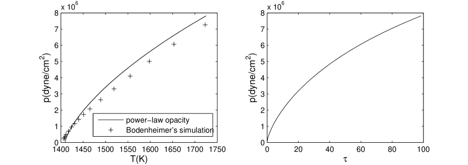
Figure 1: The structure of the uniformly irradiated equilibrium reference state for the radiative layer of HD 209458b. In the left panel, the data from Bodenheimer’s simulation (cross points) based on the opacity table by Freedman et al. 2008 are compared to the analytical solution of eq. (14) using the power-law opacity eq. (35) (solid curve). In the right panel, the relation between the pressure and the optical depth $\tau$ derived from the analytical solution is shown.

We set the positive $x$-direction as the direction of the planet’s rotation. We focus on the case that the planet is rotating faster than its orbital motion. Therefore the thermal forcing and the thermal tides propagate in a retrograde sense; i.e., the substellar point moves backwards in the frame of the rotating planet ($\omega<0$).

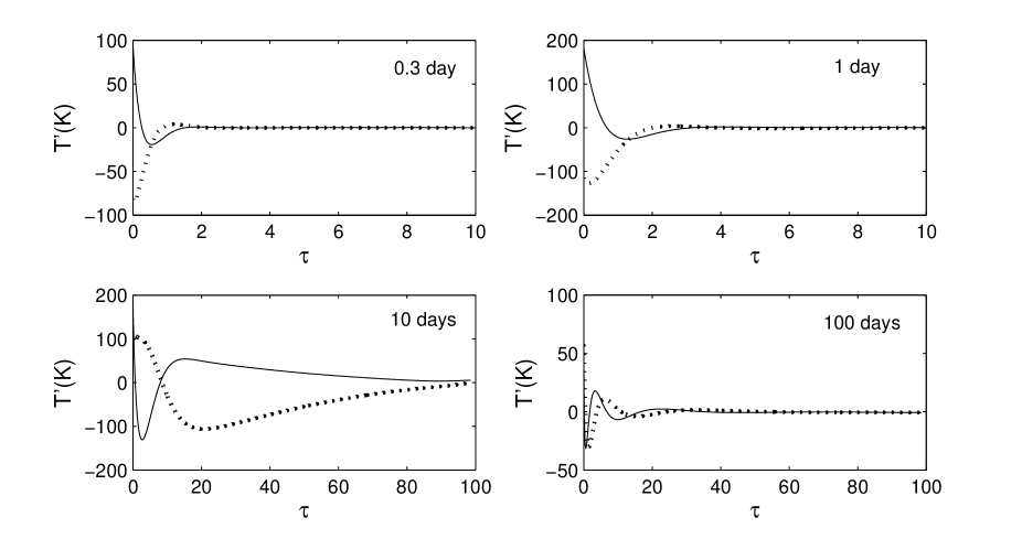
Figure 2: Temperature perturbation $T^{\prime}$ as a function of $\tau$ for the cases of 4 different forcing periods: $-2\pi/\omega=$ 0.3, 1, 10, and 100 days. The real and imaginary parts of $T^{\prime}$ are denoted by a solid and a dotted curve respectively.

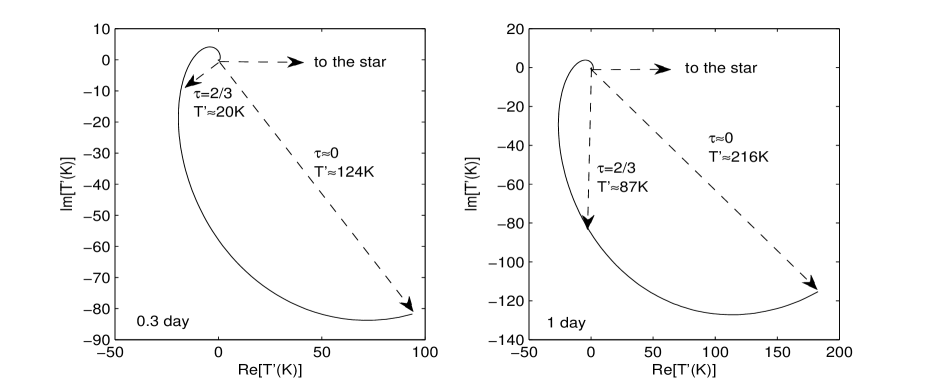
Figure 3: Phase diagrams of $T^{\prime}$ in the complex-number plane for the cases of two forcing periods: 0.3 day (left panel) and 1 day (right panel). The phase vector $T^{\prime}$ spirals clockwise from $\tau\approx 0$ to large $\tau$, meaning that $T^{\prime}$ exhibits a larger phase lag with respect to the star (i.e. the direction of the thermal forcing as shown pointing to the right in the horizontal direction) as $\tau$ increases, its magnitude decreasing and finally dropping to zero. The phase vector $T^{\prime}$ for $\tau\approx 0$ (i.e. at the top of the atmosphere) and $\tau=2/3$ (i.e. at the photosphere) are shown.

Figure 2 shows the vertical structure of $T^{\prime}$ in units of K for different thermal forcing periods $2\pi/\omega$ ranging from 0.3 day (a case for a fast rotating planet) to 100 days (a case close to the synchronous state). The real and imaginary parts of $T^{\prime}$ are denoted by a solid and a dotted curve respectively. Although the results show that $|T^{\prime}|\ll T$ in all cases, $|dT^{\prime}/dz|$ is not smaller than $|dT/dz|$ especially at small $\tau$ owing to the nonlinear forcing (i.e. $|F^{\prime}_{i}|\sim F_{i}$ at the top boundary). Therefore our linear analysis is less justified.

When the forcing periods are short (e.g. 0.3 and 1 day as shown in the top two panels), $T^{\prime}$ decays with depth and the solutions behave like those to the thermal diffusion problem with the heat diffusing from the top of the atmosphere to a depth characterized by the diffusion length $\approx\sqrt{2D/|\omega|}$, where $D$ is the thermal diffusion coefficient of the atmosphere. Comparing the 0.3-day to the 1-day case, Figure 2 shows that $T^{\prime}$ can penetrate deeper in the 1-day case as a result of a longer forcing period and therefore a longer diffusion length. The phenomenon of thermal diffusion can be also verified by the phase diagram of the complex number $T^{\prime}$. Figure 3 shows that in the cases of the forcing periods $=0.3$ and 1 day, the solutions for $T^{\prime}$, denoted by the solid curve in the real complex plane, spiral clockwise toward the origin as $\tau$ increases. The direction of the thermal forcing is shown by the horizontal arrow pointing to the right. For the forcing $\propto\exp({-i\omega t})$ with $\omega<0$, this means that the peak value of the perturbed temperature $|T^{\prime}|$ exhibits a phase lag (i.e. delay) with respect to the star. Furthermore, while the phase lag increases with depth, $|T^{\prime}|$ decreases with depth. All of these results demonstrate the process of thermal diffusion.

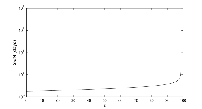
Figure 4: The Brunt–Väisälä frequency as a function of $\tau$ resulting from the vertical structure with the use of the power-law opacity shown in Figure 1. In this case, convection occurs when $\tau_{conv}\approx 98.5$.

On the other hand, when the forcing periods are long (e.g. 10 and 100 days as shown in the bottom panels of Figure 2), the vertical profiles of $T^{\prime}$ exhibit wavelike solutions, meaning that waves are excited from the top of the atmosphere and propagate in. These waves are known as internal waves (i.e. g modes). The dispersion relation of g-mode oscillation in the WKB linear perturbation analysis without dissipation reads

$$k_{x}^{2}+k_{z}^{2}={N^{2}\over\omega^{2}}k_{x}^{2},$$ (36)

where $k_{x}$ and $k_{z}$ are the horizontal and the vertical wave numbers respectively. Figure 4 shows the vertical profile of $N$ for our parameters for the radiative layer of HD 209458b. $N\gg|\omega|$ throughout the radiative layer except for the region very close to $\tau=\tau_{conv}\approx 98.5$. The dispersion relation indicates that for a given $k_{x}$, the vertical wavelength $2\pi/k_{z}$ decreases with the forcing period $2\pi/\omega$. Furthermore, internal waves can be dissipated due to radiative loss especially in the top layer of the radiative zone where the thermal timescale is short and $k_{z}$ is large. The shorter the wavelength is, the faster the wave is radiatively dissipated. This is exactly what is shown in the bottom panels of Figure 2. The internal wave for the 100-day case has a much shorter wavelength and hence decays faster with depth than the wave for the 10-day case.

The different dynamics appearing in the cases of short (thermal diffusion) and long (g mode) forcing periods can be also understood by comparing the forcing period with the sound crossing time of the planet’s surface. When the forcing period is longer than the sound crossing time of the planet’s surface; i.e.,

$${2\pi\over|\omega|}>{\pi\over k_{x}c_{sp}}={\pi R_{p}\over c_{sp}}\approx 1.5\left({R_{p}\over 1.32R_{j}}\right)\left({T\over 1500{\rm K}}\right)^{-1/2}\left({\mu\over 2}\right)^{-1/2}\ {\rm days},$$ (37)

downward-travelling internal waves (incompressible modes) can be driven by the diurnal forcing. On the other hand, when $|\omega|>k_{x}c_{sp}/2$, the day-side and the night-side are causally disconnected. The diurnal forcing results only in the thermal diffusive effect in the vertical direction.

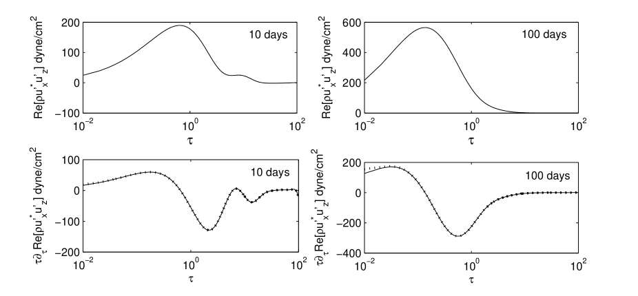
Figure 5: The top two panels show the momentum flux Re[$\rho{u^{\prime}_{x}}^{*}u_{z}^{\prime}$] as a function of $\tau$ for the cases of two forcing periods: 10 (left panel) and 100 (right panel) days. In the bottom two panels, the gradient of the momentum flux multiplied by $\tau$, denoted by the dotted curve, is plotted for comparison with the solid curve described by the right-hand side of eq. (38).

In the plane-parallel case, internal waves carry a vertical flux of horizontal momentum. This flux builds up in the upper layers of the atmosphere where the waves are thermally forced, and is reduced at greater depth where the waves are radiatively damped and transfer their momentum to the atmosphere. It can be shown from the linearized equations (27)-(30) that the gradient of the vertical momentum flux density is related to the non-adiabatic term $\nabla\cdot{\mn@boldsymbol{F}}^{\prime}$ as follows:

$$\tau\partial_{\tau}\left[{\rm Re}(\rho u^{\prime}_{x}{u^{\prime}_{z}}^{*})\right]=-\frac{\tau k_{x}}{\kappa\rho\omega}{\rm Re}\left[\frac{(\gamma-1)}{\mathrm{i}\omega}\left(\nabla\cdot{\mn@boldsymbol{u}}^{\prime}\right)^{*}\left(\nabla\cdot{\mn@boldsymbol{F}}^{\prime}\right)\right].$$ (38)

Figure 5 shows the vertical profiles of the momentum flux Re[$\rho{u^{\prime}_{x}}^{*}u_{z}^{\prime}$] and its gradient for the cases of two forcing periods: 10 and 100 days. The bottom two panels indicate that the gradient of the momentum flux, which has been multiplied by $\tau$ for clearer illustration, agrees with the right-hand side of eq. (38). This validates the relation between momentum transfer and radiative damping in our result. General speaking, both cases indicate that the momentum flux is positive and indicate that the momentum is transported from the inner region where the gradient of the momentum flux is negative to the outer region where the gradient of the momentum flux is positive. In other words, the downward-travelling internal waves excited by the thermal forcing transport momentum outward. In the 10-day case, however, the situation is more complicated since the internal waves can penetrate deeper as a result of less damping due to longer vertical wavelength (see Figure 2).

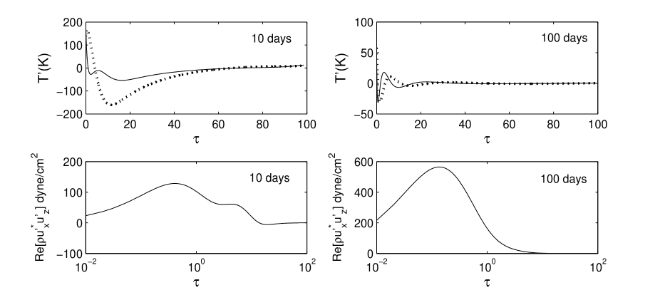
Figure 6: Vertical profiles of $T^{\prime}$ (the solid and the dotted curve denote the real and imaginary part respectively) and the vertical momentum flux Re[$\rho{u^{\prime}_{x}}^{*}u_{z}^{\prime}$] for $2\pi/\omega$=10 and 100 days based on the following bottom conditions at $\tau_{conv}$: $p^{\prime}/p=\gamma\rho^{\prime}/\rho$ and the Lagrangian density perturbation =0.

We note that the undamped internal waves in the 10-day case reach the turning point where $N=\omega$ (and therefore $k_{z}=0$) near the radiative-convective boundary (see eq. (36)). The waves are evanescent beyond the turning point and are reflected so as to interfere with the downward-travelling waves. As is clear from Figure 4, the turning point is extremely close to the bottom of the radiative layer, implying that internal waves may not be evanescent significantly at $\tau_{conv}$ where we nevertheless have imposed the boundary conditions $p^{\prime}=T^{\prime}=0$. The consequence is that the solution in the 10-day calculation is sensitive to the bottom boundary conditions at $\tau_{conv}$. To demonstrate this point, we consider the possibility that the perturbations at $\tau_{conv}$ may still preserve both the adiabatic and incompressible properties of internal waves instead of the “decaying” conditions $p^{\prime}=T^{\prime}=0$. We apply alternative bottom boundary conditions to the 10- and 100-day cases: $p^{\prime}/p=\gamma\rho^{\prime}/\rho$ (adiabatic perturbation) and the Lagrangian density perturbation =0 (incompressible perturbation). The results are shown in Figure 6. Comparing with Figure 2 and Figure 5, we find that the solutions in the 100-day case are almost the same despite different bottom boundary conditions. However, the solutions in the 10-day case are indeed different for different bottom boundary conditions. Setting the bottom boundary conditions $p^{\prime}=T^{\prime}=0$ at a location well below $\tau_{conv}$ should give rise to more reasonable solutions for the 10-day case, but would require a method of treating the dynamics in the convective zone.

The direction of momentum transport is related to the sign of $\omega$. A retrograde thermal forcing ($\omega<0$) leads to upward momentum transport. When the sign of $\omega$ is switched to positive (i.e. the planets spins slowly than the orbit), our result shows that internal waves transport momentum downwards.

3 Thermal tides in a rotating planetary atmosphere

We now consider the linearized dynamics of a thin spherical shell (a planetary atmosphere) which rotates at the uniform angular velocity $\Omega$. We adopt the coordinates $(\theta,\phi,z)$, where $\theta$ and $\phi$ are the spherical polar angles and $z$ is the altitude. In order to separate the variables and determine the solutions, we consider the “perturbations” to refer to time- and azimuth-dependent deviations from a spherically symmetrically irradiated atmosphere. This procedure corresponds to neglecting the latitudinal dependence of the average irradiation, and therefore eliminates winds in the basic state. Similar to the results for the plane-parallel case described in the preceding section, the damping of the vertically propagating waves should be able to transport and deposit angular momentum between different altitudes.

3.1 Linearized Equations

We adopt the linearized equations

$$-\mathrm{i}\omega u_{\theta}^{\prime}-2\Omega\cos\theta\,u_{\phi}^{\prime}=-\frac{1}{\rho R_{p}}\partial_{\theta}p^{\prime},$$ (39)

$$-\mathrm{i}\omega u_{\phi}^{\prime}+2\Omega\cos\theta\,u_{\theta}^{\prime}=-\frac{\mathrm{i}mp^{\prime}}{\rho R_{p}\sin\theta},$$ (40)

$$0=-\frac{1}{\rho}\partial_{z}p^{\prime}+\frac{\rho^{\prime}}{\rho^{2}}\partial_{z}p,$$ (41)

$$-\mathrm{i}\omega\rho^{\prime}+u_{z}^{\prime}\partial_{z}\rho+\rho\Delta=0,$$ (42)

$$-\mathrm{i}\omega p^{\prime}+u_{z}^{\prime}\partial_{z}p+\gamma p\Delta=-(\gamma-1)\partial_{z}F_{z}^{\prime},$$ (43)

$$F_{z}^{\prime}=F_{z}\left(\frac{\partial_{z}T^{\prime}}{\partial_{z}T}+\frac{3T^{\prime}}{T}-\frac{\rho^{\prime}}{\rho}-\frac{\kappa^{\prime}}{\kappa}\right),$$ (44)

$$\frac{p^{\prime}}{p}=\frac{\rho^{\prime}}{\rho}+\frac{T^{\prime}}{T},$$ (45)

$$\Delta=\frac{1}{R_{p}\sin\theta}\partial_{\theta}(u_{\theta}^{\prime}\sin\theta)+\frac{\mathrm{i}mu_{\phi}^{\prime}}{R_{p}\sin\theta}+\partial_{z}u_{z}^{\prime},$$ (46)

where all perturbations have the form

$$\mathrm{Re}\left[{\mn@boldsymbol{u}}^{\prime}(\theta,z)\,\mathrm{e}^{\mathrm{i}m\phi-\mathrm{i}\omega t}\right],$$ (47)

etc. We have assumed vertical hydrostatic balance and neglected horizontal radiative diffusion. These assumptions are identical to those made for the plane-parallel model and are justified in the Appendix. We have adopted the traditional approximation, which neglects $2\Omega\sin\theta\,u_{z}^{\prime}$ in the $\phi$-momentum equation. The traditional approximation is valid if $|u_{z}^{\prime}|\ll|u_{\theta}^{\prime}|,|u_{\phi}^{\prime}|$ as expected in the atmosphere where the wave frequency is much smaller than $N$. Under these assumptions we can solve the horizontal components of the equation of motion for $u_{\theta}^{\prime}$ and $u_{\phi}^{\prime}$ and substitute into the expression for $\Delta$ to obtain

$$\Delta=-\frac{1}{\mathrm{i}\omega\rho R_{p}^{2}}\mathcal{L}p^{\prime}+\partial_{z}u_{z}^{\prime},$$ (48)

where $\mathcal{L}$ is the Laplace tidal operator defined by

$$\mathcal{L}p^{\prime}=-\frac{1}{\sin\theta}(\partial_{\theta}+\nu m\cot\theta)\left[\left(\frac{\sin\theta}{1-\nu^{2}\cos^{2}\theta}\right)(\partial_{\theta}-\nu m\cot\theta)p^{\prime}\right]+\frac{m^{2}p^{\prime}}{\sin^{2}\theta},$$ (49)

with $\nu=2\Omega/\omega$ and in general, $\omega=m(n_{orb}-\Omega)$. Together with regularity conditions at the north and south poles, this is a self-adjoint operator with real eigenvalues $\lambda$ (either positive or negative) depending on the dimensionless wave frequency $\nu$. In the non-rotating limit $|\nu|\ll 1$ the eigenfunctions are associated Legendre polynomials (i.e. spherical harmonics) $P^{m}_{n}(\cos\theta)$ and the eigenvalues are $n(n+1)$ for integers $n\geq|m|$; more generally the eigenfunctions are the Hough functions $H_{\nu,m,n}(\theta)$. It is traditional to express the eigenvalues in terms of an ‘equivalent depth’ $h$:

$$\mathcal{L}H_{\nu,m,n}=\lambda_{\nu,m,n}H_{\nu,m,n}=\frac{\omega^{2}R_{p}^{2}}{gh_{\nu,m,n}}H_{\nu,m,n}.$$ (50)

We may then assume that all perturbations other than $u_{\theta}^{\prime}$ and $u_{\phi}^{\prime}$ (which have been eliminated) depend on $\theta$ through a particular Hough function. This allows for the separation of variables and we are left with the following system of ordinary differential equations:

$$0=-\frac{1}{\rho}\partial_{z}p^{\prime}+\frac{\rho^{\prime}}{\rho^{2}}\partial_{z}p,$$ (51)

$$-\mathrm{i}\omega\rho^{\prime}+u_{z}^{\prime}\partial_{z}\rho+\rho\Delta=0,$$ (52)

$$-\mathrm{i}\omega p^{\prime}+u_{z}^{\prime}\partial_{z}p+\gamma p\Delta=-(\gamma-1)\partial_{z}F_{z}^{\prime},$$ (53)

$$\Delta=-\frac{\lambda}{\mathrm{i}\omega R_{p}^{2}}\frac{p^{\prime}}{\rho}+\partial_{z}u_{z}^{\prime},$$ (54)

$$F_{z}^{\prime}=F_{z}\left(\frac{\partial_{z}T^{\prime}}{\partial_{z}T}+\frac{3T^{\prime}}{T}-\frac{\rho^{\prime}}{\rho}-\frac{\kappa^{\prime}}{\kappa}\right),$$ (55)

$$\frac{p^{\prime}}{p}=\frac{\rho^{\prime}}{\rho}+\frac{T^{\prime}}{T},$$ (56)

in which $\mathcal{L}$ has been replaced with the appropriate eigenvalue $\lambda$. These are identical to the equations used for the non-rotating plane-parallel atmosphere and lead to the same ODEs (eq. (27)-(30)) except that the horizontal wavenumber $k_{x}$ is replaced by the Hough eigenvalue $\lambda$ according to the formula $k_{x}^{2}=\lambda/R_{p}^{2}$ (or by the equivalent depth of the Hough function according to the formula $k_{x}^{2}=\omega^{2}/gh$). In the non-rotating limit this means $k_{x}^{2}=n(n+1)/R_{p}^{2}$, but in the rotating case $k_{x}^{2}$ can be positive (wave solutions) or negative (evanescent solutions).

A WKB analysis of the above linearized equations, in which $(1/r)\partial_{\theta}$ and $\partial_{r}$ are replaced by $\mathrm{i}k_{\theta}$ and $\mathrm{i}k_{r}$, gives the dispersion relation for adiabatic perturbations (Ogilvie & Lin, 2004)

$$k_{r}^{2}=\frac{N^{2}}{\omega^{2}}\left(\frac{\lambda}{r^{2}}\right),$$ (57)

where

$$\frac{\lambda}{r^{2}}\approx\frac{k_{\theta}^{2}}{1-\nu^{2}\cos^{2}\theta}.$$ (58)

This suggests that the solutions are oscillatory for $\lambda(1-\nu^{2}\cos^{2}\theta)>0$. For solutions with $\lambda>0$, the oscillations are confined to the equatorial region. This corresponds to the g-mode solutions modified by rotation (Longuet-Higgins, 1968; Bildsten et al., 1996). However, if $\lambda$ is small, this confinement is relatively weak because $k_{\theta}$ is imaginary but small away from the equatorial region. The WKB analysis in the $\theta$ direction starts to fail in this regime but the radial (i.e. vertical) wavelength can remain small if $\omega$ is very small. The solutions in this regime give rise to the baroclinic Rossby waves, or so called buoyant r modes (Longuet-Higgins, 1968; Heyl, 2004). In the limit of solutions with very small, or zero, $\lambda$, the radial WKB approach also fails. These special solutions that are global in both $r$ and $\theta$ are conventionally referred to as the barotropic Rossby waves, or simply the Rossby waves or r modes. Of course, our thin-layer calculation has eliminated barotropic r modes and we shall see later that non-adiabatic effects such as thermal diffusion affect the vertical structure of these modes to some extent.

The above description of the solution properties implies that $k_{x}$ is not simply related to the horizontal scale of the tidal forcing, as in the non-rotating problem. There is a need for reinterpretation by finding the eigenvalues of the relevant Hough functions excited by the tidal forcing. The Hough functions for a given $m$ and $\nu$ can be decomposed in terms of normalized associated Legendre polynomials $\tilde{P}_{l}^{m}$. (Ogilvie & Lin, 2004) show that the $n$th eigenvector of a certain tridiagonal matrix provides the $n$th Hough function in the form

$$H_{\nu,m,n}(\theta)=\sum_{l}a_{n,l}\tilde{P}_{l}^{m}(\cos(\theta))$$ (59)

for some coefficients $a_{n,l}$ (the components of the eigenvector $n$). In the next subsection, we shall demonstrate how we determine the relevant Hough modes excited by thermal forcing and describe the associated problem with the method of separation of variables.

3.2 Thermal Forcing

Although the parent star is not distant from its hot Jupiter, we simplify matters by assuming the stellar irradiation to consist of parallel light rays impinging on the spherical planet. The stellar irradiation (heating term) is then proportional to eq. (33) multiplied by $\sin\theta$ with $\tilde{\phi}=\phi-(n_{orb}-\Omega)t$.

The latitudinal dependence $\sin\theta$ should be decomposed into Hough functions. If the Hough functions are expressed in a basis of associated Legendre polynomials with $m=1$, it is necessary to decompose $\sin\theta$ similarly:

$$\sin\theta=-(2/\sqrt{3})\tilde{P}_{1}^{1}(\cos\theta)=-(2/\sqrt{3})\sum_{n}b_{1,n}H_{\nu,1,n}(\theta),$$ (60)

where $b_{1,n}$ is the first row of $b_{l,n}$ which is the inverse matrix of $a_{n,l}$ in eq. (59). The coefficient $b_{1,n}$ tells us how much each Hough mode is excited by the latitude-dependent irradiation with $m=1$ (i.e. the second term on the right hand side of eq. (33)).

Having said that the Hough modes are determined from the latitude-dependent heating in our model, we should note that our description is not entirely self-consistent because we have neglected the latitudinal dependence of the average irradiation. The $\theta$-dependence of $F_{i}$ would lead to a latitudinal variation of the properties of the unperturbed atmosphere and would also generate winds in the basic state. These complications are in conflict with the method of separation of variables used for solving the linear problem. However, as we have explained in the preceding subsection and as we shall see from some examples later in this paper, the Hough functions in some cases peak at low latitudes and decay quickly at high latitudes. Moreover, the latitudinal dependence of $F_{i}$, $\sin\theta$, is not a fast varying function of low latitudes. These imply that if we aim to perform an order-of-magnitude estimate of some wave quantities integrated over all latitudes (such as the vertical angular momentum flux computed later in this paper), the contribution of calculations from high latitudes should be quite small. Therefore, we may simply apply the unperturbed heating at the equator to all latitudes and expect that the error introduced from high latitudes will be diminished by the Hough functions. This allows us to consider the “perturbations” referring to time- and azimuth-dependent deviations from the symmetrically irradiated atmosphere even though the excited Hough modes are still determined by the latitude-dependent perturbed heating in our model.

3.3 Numerical Results

We adopt the same input parameters for HD 209458b in the rotating case as in the plane-parallel case to solve the linear problem. We consider the diurnal thermal forcing ($m=1$) and the scenario where the planet rotates faster than its orbit ($\omega<0$). The Hough functions and eigenvalues are obtained based on Ogilvie & Lin (2004). We only consider the $n$th “wave” mode (i.e. $\lambda>0$) which contributes the largest value of $b_{1,n}$; namely, the largest heating term in the basis of Hough functions excited by the latitude-dependent diurnal forcing. This particular $n$ is denoted as $n^{\prime}$. Then we find that the positive eigenvalue $\lambda$ associated with the leading Hough mode for $m=1$ has distinct features between fast and slow thermal tides (Longuet-Higgins 1968).

When $-2\pi/\omega$ is shorter than $\approx 7.04$ days (i.e. $<3$ times the spin period or say $-\nu<6$), $\lambda$ increases with the forcing period and is much larger than 1. The dominant Hough modes in this fast-tide regime have negative $\lambda$ and are evanescent. Positive and large $\lambda$ are then associated with less dominant Hough modes which normally consist of more weight from the associated Legendre polynomials of higher degrees. For instance, $\lambda$ for the forcing period $=0.3$, 1, 3.5, and 7 days are 37.64, 53.9, 135, and 309 respectively. The corresponding eigenvectors $H_{\nu,1,n^{\prime}}$ in the basis of the associated Legendre polynomials with the normalization coefficient $\sqrt{[(2l+1)(l-1)!]/[2(l+1)!]}$ summed from $l=1,3,5$ up to 25 are depicted in Figure 7. These latitudinal structures agree roughly with the WKB analysis described by eqs. (57) and (58): as the forcing period increases, the oscillatory solutions are more equatorially confined and the latitudinal wavelength becomes shorter. These waves excited by the fast thermal tides are g modes modified by rotation.

Figure 7: Hough functions $H_{\nu,m=1,n=n^{\prime}}(\theta)=\sum_{l=1}^{l=25}a_{n^{\prime},l}\tilde{P}_{l}^{1}(\cos\theta)$ for $-2\pi/\omega=0.3$ ($\nu\approx-2.17$, solid curve), $1$ ($\nu\approx-2.57$, dashed curve), $3.5$ ($\nu\approx-4$, dotted curve), and $7$ ($\nu=-5.97$, dash-dotted curve) days.

When the forcing period is exactly 3 times the spin period, $\lambda=0$ and the solution of the Laplace tidal equations without thermal diffusion corresponds to a $m=1$ Rossby wave with the latitudinal profile $\propto\sin\theta(1+4\cos^{2}(\theta))$. When the forcing period $>$ 3 times the spin period, other than allowing solutions with a very large positive $\lambda$ (i.e. equatorially confined g modes), the tidal equations also admit solutions with a small yet positive $\lambda$. They are known as the barotropic and baroclinic Rossby waves. These new solutions in the slow-tide regime are the predominant modes excited by the thermal forcing in our model. The $\lambda$ of the r modes increases slowly with the forcing period but remains smaller than 1. For instance, the $\lambda$ of the r modes for the forcing period $=10$, 50, 100, and 150 days are approximately 0.056, 0.109, 0.11, and 0.111 respectively. The Hough functions for these cases are plotted in Figure 8 to illustrate how the latitudinal structure of these dominant modes varies with the forcing period. Note that the r modes are less equatorially confined than the g modes and therefore couple better with the global heating profile ($\propto\sin\theta$). This explains why the r modes are more strongly excited than the g modes in our model.

Figure 8: Hough functions $H_{\nu,m=1,n=n^{\prime}}(\theta)=\sum_{l=1}^{l=25}a_{n^{\prime},l}\tilde{P}_{l}^{1}(\cos\theta)$ for $-2\pi/\omega=10$ ($\nu\approx-7.67$, solid curve), $50$ ($\nu\approx-30.4$, dashed curve), $100$ ($\nu\approx-58.7$, dotted curve), and $150$ ($\nu=-87.1$, dash-dotted curve) days.

Knowing the eigenvalues $\lambda$ and assuming the unperturbed irradiation to be spherically symmetrical, we can solve for the $z$-dependence of the perturbations. For comparison, we start our study with the rotating cases for the same forcing periods considered in the non-rotating cases: 0.3, 1, 10, and 100 days. The results for the temperature perturbations are shown in Figure 9 (rotating cases) for comparison with Figure 2 (non-rotating plane-parallel cases). In the 0.3-day case, the solutions for both the rotating and non-rotating cases exhibit diffusive behaviour. In the 100-day case, the waves propagate downwards in the rotating case as in the non-rotating case but the vertical wavelength in the rotating cases is longer (therefore the waves are less damped via radiative loss) because $\lambda$ has a small value. However in the 1-day and 10-day cases, the Coriolis effect introduces a large and a small $\lambda$ respectively, turning the diffusive solution to a wave solution in the 1-day case and turning the wave solution to a diffusive solution in the 10-day case.

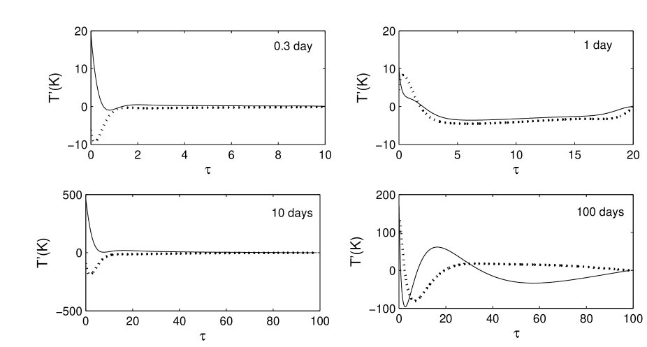
Figure 9: Same as Figure 2 except that the Coriolis effect is included.

Although the leading modes in the 0.3- and 10-day cases give rise to vertically diffusive solutions, the less dominant modes (with therefore smaller magnitudes), do admit vertical wave solutions due to the much larger values of $\lambda$. These are g modes and more equatorially confined. For instance, we find that (not plotted here) the second dominant mode in the 10-day case gives a vertical wave solution (g mode) because $\lambda\approx 535$ but its wave magnitude, described by $b_{1,n}$, is 0.024 which is much smaller than the magnitude $b_{1,n^{\prime}}=0.905$ of the most dominant mode. The Hough function in the 10-day case has a latitudinal profile close to $\sin\theta(1+4\cos^{2}(\theta))$, more akin to the barotropic Rossby mode. On the other hand, the dominant modes for the forcing period $>20$ days do give vertical wave solutions. As the planet is more rotationally synchronized (i.e., $-\omega$ becomes smaller and therefore $-\nu$ becomes larger), the Rossby waves are more akin to baroclinic r modes with shorter vertical wavelength (see the 100-day case in Figure 9) and are more equatorially confined. Note that although the r mode in the 10-day case decays vertically due to thermal diffusion, it has a broad distribution across latitudes. Therefore the assumption of symmetrical unperturbed irradiation relying on small values of Hough functions at high latitudes may not be appropriate in this case.

In the regime of fast thermal tides ($-\nu<6$), only g modes can exist. In the 1-day case, we have applied the bottom boundary conditions $p^{\prime}=T^{\prime}=0$ at $\tau=20$ to illustrate the results (see Figure 9) because we have difficulty obtaining the solutions when imposing the bottom boundary conditions at $\tau=\tau_{conv}$. This may result from the possibility that the wave of long vertical wavelength in the 1-day case can penetrate deep into the radiative layer, rendering the bottom boundary conditions $p^{\prime}=T^{\prime}=0$ invalid (cf. the 10-day case in the non-rotating case). To justify this approach for the 1-day case, we examine the solutions for forcing periods slightly longer than 1 day, with the expectation that short-wave solutions would appear owing to the larger $\lambda$. This is illustrated in Figure 10 for the cases of $-2\pi/\omega=3.5$ days ($\lambda\approx 135$) and $7$ days ($\lambda\approx 309$). As the forcing period increases from 1 day to 3.5 days, and then to 7 days, the wave solutions can be seen clearly with decreasing vertical wavelength, as expected. The larger values of $\lambda$ associated with the less dominant Hough modes manifest themselves as shorter latitudinal wavelength as a result of the Coriolis effect, driving internal waves of shorter vertical wavelength according to the WKB dispersion relation (see eqs. (57) and (58)).

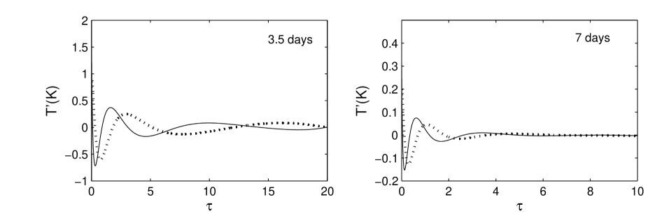
Figure 10: Same as Figure 9 but for the rotating cases of $-2\pi/\omega=3.5$ days and $7$ days.

In summary, the diurnal thermal forcing in the rotating case excites a series of Hough modes. When the forcing period is long (i.e., $-2\pi/\omega$ is much longer than $\sim 10-20$ days), the dominant modes are baroclinic Rossby waves that can propagate downwards. When the forcing period is short (i.e., $-2\pi/\omega$ is shorter than $\sim 10-20$ days), the dominant modes are evanescent due to either the Coriolis effect (i.e. negative $\lambda$) or thermal diffusion. However, the less dominant modes have short latitudinal wavelength and therefore internal waves can be excited without being subject to the same constraint that the sound crossing time between the day and night sides needs to be shorter than the forcing period as in the non-rotating plane-parallel case. Since the less dominant modes are small in magnitude, we expect that the angular momentum transported by the fast tides (g modes) is smaller than in the case of the slow tides (r modes). This is the subject of the next subsection.

3.4 Vertical Angular Momentum Transport

The vertical angular momentum flux carried by the Hough waves integrated over the planet’s surface is given by (Ogilvie & Lin, 2004)

$$L=\frac{\pi m}{\omega}\int_{0}^{\pi}{\rm Re}[{p^{\prime}}^{*}u^{\prime}_{z}]R_{p}^{2}\sin\theta d\theta,$$ (61)

where $p^{\prime}$ and $u^{\prime}_{z}$ are both expressed as series of Hough functions ($p^{\prime}=\sum_{n}p^{\prime}_{n}H_{\nu,m,n}$, etc.) in our model. Then the total flux is the sum of the contributions from each Hough function, because they are orthogonal. Therefore, the angular momentum flux carried by each Hough mode $H_{\nu,m,n}$ with $m=1$ is given by

$$L_{n}=\frac{\pi}{\omega}\int_{0}^{\pi}{\rm Re}[{p^{\prime}_{n}}^{*}u^{\prime}_{zn}]H_{\nu,m=1,n}^{2}R_{p}^{2}\sin\theta d\theta=\frac{\pi}{\omega}{\rm Re}[{p^{\prime}_{n}}^{*}u^{\prime}_{zn}]R_{p}^{2},$$ (62)

where we have used the normalization $\int_{0}^{\pi}H_{\nu,m,n}^{2}\sin\theta d\theta=1$. We focus only on $L_{n}$ due to the leading Hough mode (i.e., $n=n^{\prime}$) and use the peak value of the radial profile of the angular momentum flux to quantify the torque in each case of parameter study.

Since our calculation is limited to a thin radiative layer and by the condition of symmetrical unperturbed irradiation, to reasonably estimate $L_{n^{\prime}}$, we focus on the frequency regimes in which the solutions give short vertical wavelengths and modest equatorial confinement. Hence we carry out the estimates for the following forcing periods: 3.5, 7, 100, & 150 days. The results are listed in Table 1, taking into consideration 4 different cases for each forcing period; Case I: the original case for the input parameters of HD 209458b, Case II: the same input parameters as Case I except that a larger $\kappa$ ($c_{\kappa}$ is increased by a factor of 100) is used, Case III: the same as Case I except that a larger $R_{p}$ ($=2R_{J}$, a young planet) is used, and Case IV: the same as Case I except that a smaller $a$ (one half of $0.0474$ AU) is used. Note that changing $\kappa$, $R_{p}$, or $a$ would alter the interior structure and therefore other input parameters such as $F_{z}$ need to change accordingly. However, the purpose of the present case study here is simply to investigate how $L_{n^{\prime}}$ varies with each parameter and to better understand what we can expect from our model for other interesting cases.

In general, Table 1 shows that the torques in the fast-tide cases (i.e. 3.5 and 7 days) are weaker than those in the slow-tide cases (i.e. 100 and 150 days) by several orders of magnitude. As described in the previous subsection, this is primarily because the dominant Hough modes in the fast-tide regime are evanescent in the vertical direction. More specifically, the amplitudes of the internal waves $|b_{1,n^{\prime}}|$ are 0.08 for $2\pi/\omega=-3.5$ days and 0.04 for $2\pi/\omega=-7$ days, which are smaller than the amplitudes of the baroclinic Rossby waves 0.88 for $2\pi/\omega=-100$ days and 0.82 for $2\pi/\omega=-150$ days.

Table 1 also illustrates how different input parameters affect the torque $L_{n^{\prime}}$ driven by the thermal tides. Case II shows that increasing $c_{\kappa}$ by 2 orders of magnitude only reduces the torque by less than a factor of 3, indicating that the result is less sensitive to the opacity. Case III shows that the torque driven by fast (i.e., 3.5 and 7 days) thermal tides on a larger hot Jupiter is weaker than that on a smaller hot Jupiter. The effect is opposite for slow (i.e., 100 and 150 days) thermal tides. Case IV shows that placing a hot Jupiter closer to its parent star decreases (increases) the torque in the fast (slow) tide case. Note that increasing $\kappa$, $R_{p}$ (therefore $g$), or $F_{i}$ reduces the pressure and density of the equilibrium state at a given $\tau$. This normally leads to an increase in $u^{\prime}_{z}$ but does not dictate the change of $p^{\prime}$ in any unique way among the various cases. Therefore, the torque does not follow a simple trend in variation with any of the input parameters.

Table 1: Torques in units of $10^{30}$ dyne cm generated by thermal tides with $2\pi/\omega=-3.5$, $-100$, and $-150$ days for 4 different cases.

Case	$-3.5$ days	$-7$ days	$-100$ days	$-150$ days
I (original)	0.062	0.014	3474	3011
II (high $\kappa$)	0.022	0.005	2276	1973
III (large $R_{p}$)	0.041	0.009	8414	7294
IV (small $a$)	0.056	0.013	13719	11893

Compared to the torque generated by the gravitational tides, the torque driven by the radiative damping of the baroclinic Rossby waves is sizable. With a constant tidal lag angle specified by the $Q^{\prime}_{p}$ value of the planet, the torque due to the gravitational equilibrium tides driven by a parent star on a non-synchronized planet is given by (e.g. Goldreich & Soter 1966)

$$L_{grav} = {3GM_{*}^{2}R_{p}^{5}\over 2a^{6}Q^{\prime}_{p}}$$ (63)

$$\approx 2.8\times 10^{32}\left({M_{*}\over 1.1M_{sun}}\right)^{2}\left({R_{p}\over 1.32R_{J}}\right)^{5}\left({a\over 0.0474{\rm AU}}\right)^{-6}\left({Q^{\prime}_{p}\over 10^{6}}\right)^{-1}\ {\rm dyne\ cm}$$ (64)

which is comparable to the torques driven by slow Hough waves listed in Table 1. This implies that in our calculation, thermal tides play a significant role in transferring angular momentum to the atmospheric gas even if contributions of the gravitational tides are also a factor in the atmosphere.

4 Summary and Discussions

We present a linear perturbation analysis for internal waves excited by the stellar diurnal thermal forcing ($m=1$ thermal tides) in a non-synchronized radiative layer of a hot Jupiter. For computational simplicity, we employ the radiative diffusion approximation with a power-law opacity throughout our computation region from the radiative layer to a cloud-free atmosphere and apply the Marshak boundary condition for energy balance at $z=+\infty$. We use the parameters of HD 209458b as an illustrative example.

We first perform a linear perturbation analysis for a non-rotating plane-parallel atmosphere to explore how the dynamics of thermal response in the atmosphere varies with the thermal forcing frequency $\omega$ in the absence of the Coriolis effect. The boundary conditions at the bottom of the radiative layer are set to be $p^{\prime}=T^{\prime}=0$ which we speculate are less accurate for the waves with long vertical wavelength. Nevertheless, we find that when the thermal forcing period is shorter than the sound speed crossing time between the day and the night sides of the planet, the periodic thermal heating at the top of the atmosphere diffuses into a deeper layer with a decay length related to $\omega$. In the fast thermal forcing regime corresponding to the rotation rate of our Jupiter, the problem for an atmosphere heated by the stellar irradiation becomes essentially a 1-D thermal diffusion problem with $k_{x}\rightarrow 0$. On the other hand, when the thermal forcing period is longer than the sound crossing time of the planet’s surface, the day and the night sides are causally connected and the problem becomes a 2-D phenomenon with incompressible properties. As a result, the internal waves are excited at the top of the atmosphere before propagating downwards. When the planet spins faster (slower) than its orbital motion, the thermal tides exhibit a retrograde (prograde) motion. The retrograde (prograde) waves causes the upward (downward) transport of momentum. The radiative damping of the waves leads to the deposition of the momentum in the atmosphere.

We then carry out a linear calculation for a thin spherical shell which rotates at a uniform angular speed. Since $|\omega|\ll N$, we adopt the traditional approximation and neglect inertial terms in the vertical momentum equation. We also assume a spherically symmetrically irradiated atmosphere as the basic state. These assumptions allow us to separate the variables and obtain the perturbation of the form Re$[u^{\prime}(z)H_{\nu,m,n}(\theta)\exp{(im\phi-i\omega t)}]$. We examine the diurnal thermal forcing $m=1$ and consider the $n$th component of the Hough function which contributes the dominant latitudinal structure of the heating. The linearized ODEs thus remain the same as those in the plane-parallel case except that the horizontal wavenumber $k_{x}$ is replaced by the eigenvalue $\sqrt{\lambda}/R_{p}$. In other words, $\lambda$ conceals the information on how the latitudinal structure is modified by the Coriolis effect. Similar to the non-rotating plane-parallel case, the internal waves are driven by thermal forcing at the top of the rotating atmosphere. However, the internal waves in most of cases are primarily confined in a band of latitudes close to the equator and therefore are weakly excited by the global thermal forcing in our model. In the slow-tide regime (i.e., $-2\pi/\omega$ is much longer than $\sim 10-20$ days), baroclinic Rossby waves can be largely excited by the global thermal forcing. When the planet spins faster than its orbit ($\omega<0$), these waves propagate inwards but transport angular momentum outwards. While the torque generated by the radiative damping of the baroclinic Rossby waves in the slow-tide regime is comparable to the torque due to the gravitational tides, the torque generated by internal waves in the fast-tide regime (i.e., $-2\pi/\omega$ is shorter than $\sim 10-20$ days) is smaller by several orders of magnitude. The magnitude of the torque is more sensitive to $R_{p}$ and $a$ than $\kappa$ in our model.

Unlike the thermal tide theories for a dense atmosphere on a terrestrial planet (Gold & Soter, 1969; Dobrovolskis & Ingersoll, 1980; Correia et al., 2003), our model for hot Jupiters, which do not have a hard surface, fails to generate net thermal bulges and therefore causes only internal transport of angular momentum inside the planet. In fact, the atmosphere in our model brings the interior closer to, not further away from, synchronous rotation. Together with the gravitational tides, one possible equilibrium state for rotation in our scenario is still the synchronous rotation.

At this point, it is not clear how our linear results without winds for a non-synchronized hot Jupiter are able to explain the vertical shear appearing in existing 3-dimensional numerical simulations for the atmospheres of hot Jupiters. Apparently, the advection in the upper atmosphere of a hot Jupiter is driven by the temperature gradient between the day and night sides and cannot be described by our linear approach. Nevertheless, it is likely that the wave dynamics plays a role in the lower atmosphere where the day-night temperature contrast is small. Cooper & Showman (2005) postulate that the equatorial super-rotating jet occurring in the deep atmosphere of HD 209458b in their simulation could be due to wave transport. The numerical simulation by Showman et al. (2008) for a non-synchronously rotating HD 209458b shows that the super-rotating jets are more equatorially confined and penetrate deeper in their case for $2\pi/\omega=-3.5$ days than those in their cases for $2\pi/\omega=7$ days and $\infty$. Whether the deeper distribution of the super-rotating jet is due to the Hough waves driven by retrograde thermal forcing is an interesting subject worthy of further investigation.

Our work presented in this paper is the first attempt at an analytical understanding of thermal tides in a hot Jupiter. Our linear theory suggests that the angular momentum transport in the atmosphere of a hot Jupiter due to a periodic thermal forcing is possible and mostly happens in low latitudes through the radiative damping of Hough waves. This encouraging result lays the foundation for further improvements in our calculations during future investigation, such as the inclusion of the semi-diurnal contribution, the consideration of Kelvin waves (third kind of Hough waves; e.g. see Longuet-Higgins 1968) driven by prograde thermal forcing, or the examination of internal waves driven from clouds in hot Jupiters. The extension of this work to other applications, for instance, thermal bulges on hot super-earths or Hough waves on a pseudo-synchronized hot Jupiter in an eccentric orbit (cf. Langton & Laughlin 2008), is necessary for gaining further insight into the question of how waves can play a role in atmospheric circulation on hot Jupiters.

Appendix A Dimensionless equations and top boundary conditions

In this section, we demonstrate how the fluid equations are non-dimensionalized in our problem. This procedure will not only help to clarify the relative importance among various terms in the equations more easily, but also shed light on the behaviour of the solutions near $\tau=0$ and help to specify the top boundary conditions.

The equilibrium and perturbed states are completely determined once the parameters $g$, $c_{\kappa}$, $a$, $b$, $\mu$, $F_{z}$ and $F_{\mathrm{i}}$ are specified. Therefore the problem can be non-dimensionalized in terms of these parameters. We can write $p=\tilde{p}\,U_{p}$, $T=\tilde{T}\,U_{T}$, $\rho=\tilde{\rho}\,U_{\rho}$, $\kappa=\tilde{\kappa}\,U_{\kappa}$, and $z=\tilde{z}\,U_{z}$, where $\tilde{p}$, $\tilde{T}$, $\tilde{\rho}$, $\tilde{\kappa}$, a nd $\tilde{z}$ are dimensionless functions of $\tau$ and the dimensional units are given by the following relations:

$$\sigma U_{T}^{4}=F_{z},$$ (65)

$$U_{p}=\frac{g}{U_{\kappa}},$$ (66)

$$U_{p}=\frac{R}{\mu}U_{\rho}U_{T},$$ (67)

$$U_{z}=\frac{1}{U_{\kappa}U_{\rho}},$$ (68)

$$U_{\kappa}=c_{\kappa}U_{p}^{a}U_{T}^{-4b}.$$ (69)

The equilibrium solution can then be expressed as

$$\tilde{T}=\left[{\textstyle{\frac{3}{4}}}(\tau+{\textstyle{\frac{2}{3}}})+f\right]^{1/4},$$ (70)

$${\tilde{p}}^{a+1}=\frac{4}{3}\left(\frac{a+1}{b+1}\right)\left[\tilde{T}^{4(b+1)}-\tilde{T}_{\infty}^{4(b+1)}\right],$$ (71)

$$\tilde{\rho}=\frac{\tilde{p}}{\tilde{T}},$$ (72)

$$\tilde{z}=-\int\frac{1}{\tilde{p}^{a}\tilde{T}^{-4b}}\frac{\mathrm{d}\tau}{\tilde{\rho}},$$ (73)

where $f=F_{\mathrm{i}}/F_{z}$ is a dimensionless parameter that determines the importance of irradiation. A further dimensionless parameter associated with the problem is

$$\epsilon=\frac{F_{z}}{U_{p}U_{c}},$$ (74)

where $U_{c}\equiv(RU_{T}/\mu)^{1/2}$, a characteristic velocity unit. For the parameters adopted for HD 209458b in this paper, $\epsilon\approx 4.8\times 10^{-6}\ll 1$. We further define an estimate of the radiative thermal diffusivity $U_{\chi}$ as follows

$$U_{\chi}=\frac{F_{z}}{U_{\kappa}U_{\rho}U_{p}}.$$ (75)

The linearized equations (27)-(30) can also be made dimensionless by writing $\omega=\tilde{\omega}\,U_{\omega}$, $k_{x}=\tilde{k}_{x}\,U_{k}$, $\xi_{z}=\tilde{\xi}_{z}\,U_{z}$, $p^{\prime}=\tilde{p}^{\prime}\,U_{p}$, $T^{\prime}=\tilde{T}^{\prime}\,U_{T}$ and ${\mn@boldsymbol{F}}^{\prime}=\tilde{\mn@boldsymbol{F}}^{\prime}\,F_{z}$, where

$$U_{\omega}=\frac{U_{\chi}}{U_{z}^{2}},$$ (76)

$$U_{k}=\frac{U_{\omega}}{U_{c}}.$$ (77)

Note that $U_{k}U_{z}=\epsilon$. The above scaling leads to

$$\partial_{\tau}\tilde{\xi}_{z}=(\partial_{\tau}\ln\tilde{T}-\partial_{\tau}\ln\tilde{p})\tilde{\xi}_{z}-\frac{\tilde{k}_{x}^{2}\tilde{p}^{\prime}}{\tilde{\kappa}\tilde{\omega}^{2}\tilde{\rho}^{2}}+\frac{1}{\tilde{\kappa}\tilde{\rho}}\left(\frac{\tilde{p}^{\prime}}{\tilde{p}}-\frac{\tilde{T}^{\prime}}{\tilde{T}}\right),$$ (78)

$$\partial_{\tau}\tilde{p}^{\prime}=-\epsilon^{2}\frac{\tilde{\omega}^{2}\tilde{\xi}_{z}}{\tilde{\kappa}}+\frac{1}{\tilde{\kappa}}\left(\frac{\tilde{p}^{\prime}}{\tilde{p}}-\frac{\tilde{T}^{\prime}}{\tilde{T}}\right),$$ (79)

$$\partial_{\tau}\tilde{T}^{\prime}=\left[(a+1)\frac{\tilde{p}^{\prime}}{\tilde{p}}-(b+1)\frac{4\tilde{T}^{\prime}}{\tilde{T}}+\tilde{F}_{z}^{\prime}\right]\partial_{\tau}\tilde{T},$$ (80)

$$\partial_{\tau}\tilde{F}_{z}^{\prime}=\tilde{p}\left[\left(\frac{\gamma}{\gamma-1}\right)\partial_{\tau}\ln\tilde{T}-\partial_{\tau}\ln\tilde{p}\right]\mathrm{i}\tilde{\omega}\tilde{\xi}_{z}+\epsilon^{2}\frac{\tilde{k}_{x}^{2}\tilde{T}^{\prime}}{\tilde{\kappa}^{2}\tilde{\rho}^{2}\partial_{\tau}\tilde{T}}$$

$$+\frac{\mathrm{i}\tilde{\omega}\tilde{p}}{\tilde{\kappa}\tilde{\rho}}\left[\frac{\tilde{p}^{\prime}}{\tilde{p}}-\left(\frac{\gamma}{\gamma-1}\right)\frac{\tilde{T}^{\prime}}{\tilde{T}}\right].$$ (81)

The terms proportional to $\epsilon^{2}$ may reasonably be omitted. Neglecting these small terms amounts to assuming vertical hydrostatic balance and neglecting horizontal radiative diffusion.

For $a+1>0$, we find the behaviour of physically acceptable solutions as $\tau\to 0$ (omitting the $\epsilon^{2}$ terms) to be as follows:

$$\tilde{\xi}_{z}=\left[C_{1}+O(\tau)\right]\ln\tau+\left[C_{2}+O(\tau)\right],$$ (82)

$$\tilde{p}^{\prime}=\tau^{1\over a+1}\left[C_{3}+O(\tau)\right]\ln\tau+\tau^{1\over a+1}\left[C_{4}+O(\tau)\right],$$ (83)

$$\tilde{T}^{\prime}=\left[C_{5}\tau+O(\tau^{2})\right]\ln\tau+\left[C_{6}+O(\tau)\right],$$ (84)

$$\tilde{F}_{z}^{\prime}=\tau^{1\over a+1}\left[C_{7}+O(\tau)\right]\ln\tau+C_{8},$$ (85)

together with the background states

$$\tilde{T} = \tilde{T}_{\infty}+\tilde{T}_{1}\tau+O(\tau^{2}),$$ (86)

$$\tilde{p}^{a+1} = {\tilde{p}_{1}}\tau+O(\tau^{2}),$$ (87)

where $\tilde{T}_{\infty}=({\textstyle{\frac{1}{2}}}+f)^{1/4}$, $\tilde{T}_{1}={\textstyle\frac{3}{16}}({\textstyle{\frac{1}{2}}}+f)^{-3/4}$, and $\tilde{p}_{1}=(a+1)({\textstyle{\frac{1}{2}}}+f)^{b}$. The only variable to diverge as $\tau\to 0$ is $\tilde{\xi}_{z}$, but since $\tilde{\rho}=\tilde{p}/\tilde{T}=O(\tau^{1\over a+1})$, the mass flux at $\tau=0$ vanishes. In fact the $\epsilon^{2}$ terms eventually become important as $\tau\to 0$, but we neglect them here. On substituting these series into the ODEs, we obtain the following relations between the coefficients:

$$C_{1}=(a+1)\left(\tilde{T}_{\infty}-\frac{\tilde{k}_{x}^{2}\tilde{T}_{\infty}^{2}}{\tilde{\omega}^{2}}\right)\frac{1}{\tilde{p}_{1}^{(a+2)/(a+1)}}\left(\frac{1}{\tilde{T}_{\infty}}\right)^{-4b}C_{3}$$ (88)

$$C_{1}=-\frac{C_{2}}{a+1}+\left({\tilde{T}}_{\infty}-\frac{\tilde{k}_{x}^{2}\tilde{T}_{\infty}^{2}}{\tilde{\omega}^{2}}\right)\frac{1}{\tilde{p}_{1}^{(a+2)/(a+1)}}\left(\frac{1}{\tilde{T}_{\infty}}\right)^{-4b}C_{4}-\frac{1}{\tilde{p}_{1}}\left(\frac{1}{\tilde{T}_{\infty}}\right)^{-4b}C_{6},$$ (89)

$$C_{3}=-\frac{C_{6}}{\tilde{T}_{\infty}}\frac{1}{\tilde{p}_{1}^{a/(a+1)}}\left(\frac{1}{\tilde{T}_{\infty}}\right)^{-4b},$$ (90)

$$C_{5}=\frac{(a+1)\tilde{T}_{1}}{\tilde{p}_{1}^{1/(a+1)}}C_{3},$$ (91)

$$C_{7}=-\mathrm{i}\tilde{\omega}\tilde{p}_{1}^{1/(a+1)}C_{1}+(a+1)\mathrm{i}\tilde{\omega}\tilde{T}_{\infty}\frac{1}{\tilde{p}_{1}}\left(\frac{1}{\tilde{T}_{\infty}}\right)^{-4b}C_{3}.$$ (92)

In addition, eq. (31), the thermal forcing condition at $\tau=0$, in dimensionless terms reads

$$C_{8}=8\tilde{T}_{\infty}^{3}C_{6}-2f^{\prime},$$ (93)

where the thermal forcing term $f^{\prime}=F_{\mathrm{i}}^{\prime}/F_{z}$. As a result, all the coefficients in the series expansion of the solution can ultimately be expressed in terms of $C_{4}$ and $C_{6}$. We apply the shooting method in solving the ODEs. We can first guess the values of $C_{4}$ and $C_{6}$ and evaluate the other expansion coefficients using the above relations. We then initialize the solution at $\tau\ll 1$ and integrate to $\tau=\tau_{conv}$, where two boundary conditions can be applied to determine the values of $C_{4}$ and $C_{6}$ and therefore the values of $\tilde{\xi}$, $\tilde{p}^{\prime}$, $\tilde{T}^{\prime}$, and $\tilde{F}_{z}^{\prime}$ at $\tau\ll 1$.

References

- Bildsten et al. (1996) Bildsten L., Ushomirsky G., & Cutler C., 1996, ApJ, 460, 827
- Bodenheimer et al. (2001) Bodenheimer P., Lin D. N. C., & Mardling R. A., 2001, ApJ, 548, 466
- Bodenheimer et al. (2003) Bodenheimer P., Laughlin G., & Lin D. N. C., 2003, ApJ, 592, 555
- Cartwright (2000) Cartwright D. E., 2000, Tides (Cambridge: Cambridge Univ. Press)
- Chapman & Lindzen (1970) Chapman S. & Lindzen R., 1970, Atmospheric Tides: Thermal and Gravitational, Gordon and Breach
- Cho (2008) Cho, J. Y.-K. 2008, Phil. Trans. R. Soc. A, 366, 4477
- Cooper & Showman (2005) Cooper C. S. & Showman A. P., 2005, ApJ, 629, L45
- Correia & Laskar (2003) Correia A. C. M. & Laskar J., 2003, J. Geophysical Research, 108, 9-1
- Correia et al. (2003) Correia A. C. M., Laskar J., & Néron de Surgy O. N., 2003, Icarus, 163, 1
- Cowan et al. (2007) Cowan N. B., Agol E., & Charbonneau D., 2007, MNRAS, 379, 641
- Dobbs-Dixon & Lin (2007) Dobbs-Dixon I. & Lin D. N. C., 2008, ApJ, 673, 513
- Dobrovolskis & Ingersoll (1980) Dobrovolskis A. R. & Ingersoll A. P., 1980, Icarus, 41, 1
- Freedman et al. (2008) Freedman R.S., Marley M. S., & Lodders K., 2008, ApJS, 174, 504
- Gold & Soter (1969) Gold T. & Soter S., 1969, Icarus, 11, 356
- Goldreich & Nicholson (1989) Goldreich P., Nicholson P. D., 1989, ApJ, 342, 1079
- Guillot (2005) Guillot T., 2005, Annu. Rev. Earth Planet. Sci., 33, 493
- Harrington et al. (2006) Harrington et al., 2006, Science, 314, 623
- Haurwitz (1964) Haurwitz B., 1964, Science, 144, 1415
- Heyl (2004) Heyl J., 2004, ApJ, 600, 939
- Knutson et al. (2007) Knutson H. A., Charbonneau D., Allen L. E., Fortney J. J., Agol E., Cowan N. B., Showman A. P., Cooper C. S. & Megeath S. T., 2007, Nature, 447, 183
- Langton & Laughlin (2008) Langton J. & Laughlin G., 2008, A&A, 483, 25
- Laskar & Correia (2004) Laskar J. & Correia A. C. M., 2004, in Extrasolar Planets: Today and Tomorrow, ASP Conference Proceedings, 321, 401
- Longuet-Higgins (1968) Longuet-Higgins M. S., 1968, Phil. Trans. R. Soc. London, 262, 511
- Lubow et al. (1997) Lubow S. H., Tout C. A., & Livio M., 1997, ApJ, 484, 866
- Mardling (2007) Mardling R. A., 2007, MNRAS, 382, 1768
- Ogilvie & Lin (2004) Ogilvie G. I. & Lin D. N. C., 2004, ApJ, 610, 477
- Orton et al. (2008) Orton G. S. et al., 2008, Nature, 453, 196
- Pomraning (1973) Pomraning G. C., 1973, The equations of radiation hydrodynamics, Pergamon Press
- Showman et al. (2007) Showman A. P., Menou K., & Cho J. Y.-K., 2007, in proceedings of the Conference on Extreme Solar Systems, arXiv:0710.2930v1
- Showman et al. (2008) Showman A. P., Cooper C. S., Fortney J. J., & Marley M. S., 2008, arXiv:0802.0327v1
- Showman & Guillot (2002) Showman A. P. & Guillot T., 2002, A&A, 385, 166