BSLP: Markovian Bivariate Spread-Loss Model
for Portfolio Credit Derivatives
Matthias Arnsdorf and Igor Halperin
Quantitative Research, JP Morgan
Email: matthias.x.arnsdorf@jpmorgan.com, igor.halperin@jpmorgan.com
March 2007

Abstract:

BSLP is a two-dimensional dynamic model of interacting portfolio-level loss and loss intensity processes. It is constructed as a Markovian, short-rate intensity model, which facilitates fast lattice methods for pricing various portfolio credit derivatives such as tranche options, forward-starting tranches, leveraged super-senior tranches etc. A semi-parametric model specification is used to achieve near perfect calibration to any set of consistent portfolio tranche quotes. The one-dimensional local intensity model obtained in the zero volatility limit of the stochastic intensity is useful in its own right for pricing non-standard index tranches by arbitrage-free interpolation.

1 Introduction

A large class of portfolio credit derivatives can be viewed as derivatives referencing the cumulative portfolio losses. Furthermore, we can distinguish between two classes of such derivatives. For single-period (vanilla) instruments such as synthetic CDO tranches all that is needed for pricing is the set of marginal portfolio loss distributions at different time horizons. More exotic, multi-period instruments such as tranche options require knowledge of the future distributions of the mark-to-market (MTM) of the tranche as well as the portfolio losses. This is equivalent to having a model for the evolution of the portfolio losses, from which the MTM of the tranche can then be derived.

If we hedge such multi-period products only using tranches on the underlying portfolio, then the challenge of modeling single-name dynamics does not arise at all. Therefore, under these conditions both the pricing and risk management of portfolio credit derivatives can be done within a model that specifies the portfolio-level dynamics of cumulative losses but leaves the single name dynamics unspecified (or specified at a later stage).

The fact that powerful and flexible pricing models can be constructed within such a “top-down” framework was first recognized in work by Giesecke and Goldberg [1], Schönbucher [2], Sidenius, Piterbarg and Andersen (SPA) [3], and Bennani [4]. More recent publications along this strand include Brigo et al. [5], Chapovsky et al. [6], Errais et al. [7], Cont et al. [8], Ding et al. [9], and de Kock et al. [10]. Furthermore, while this paper was under preparation we learned of a recent paper by Lopatin and Misirpashaev [11] who have independently suggested a model similar to the one developed in this paper. We will comment on similarities and differences between their approach and ours in due course.

In this paper, we present the Bivariate Spread-Loss Portfolio (BSLP) model - a dynamic Markovian model for correlated portfolio loss and loss intensity processes. In our model the portfolio loss process follows a Markov chain whose generator is driven by a stochastic intensity (so that the generator itself becomes stochastic). The intensity is given by a diffusion process which can incorporate default-induced jumps. The fact that the driving intensity and the loss process are mutually dependent means that our framework is more general than the more standard doubly stochastic one which only allows for a one-sided dependence.

The portfolio default intensity is a derived process in our model. It is shown to be a jump-diffusion that depends on the default level. This dependence is governed by a set of multiplicative factors - the so-called contagion factors. These factors enable a convenient semi-parametric specification which can be calibrated to any set of consistent portfolio tranche quotes. Furthermore, the fact that the model is two-dimensional and Markovian means that efficient lattice implementations are available.

Our framework can be viewed as a low-dimensional short-rate version of the approach described by Schönbucher in [2]. In particular, Schönbucher describes a Heath-Jarrow-Morton (HJM)-like model of forward default transition rates which will in general be non-Markovian and require Monte-Carlo simulations. The BSLP model, on the other hand, imposes local drift conditions that allow for fast lattice implementations, as indicated above.

Both models coincide in the local intensity limit where the intensity process becomes a locally deterministic function of the default level. In this case, we obtain a continuous-time, one-dimensional Markov chain driven by a deterministic Markov generator. This can serve as a model in its own right, useful for constructing an arbitrage-free interpolation of liquid index (e.g. iTraxx or CDX) tranche prices across strikes and maturities. The interpolation can then be used to price non-standard index tranches consistently, which is often a problem in the standard base correlation framework.

This is similar to the way local volatility models are used to price exotic equity or FX options off liquid vanillas. While such a framework can formally be viewed as a dynamic model, it is known that local volatility models misspecify the dynamics of the volatility process, and are therefore ill-suited for pricing instruments sensitive to the forward smile dynamics, such as forward starting options and cliquets. This points to the need for stochastic volatility models.

Similarly, what is needed in the present context, for the pricing of multi-period credit derivatives is a stochastic evolution of the loss distribution. This is obtained by making the Markov chain generator stochastic. In this way, we arrive at the full-blown, stochastic intensity version of the BSLP model.

Besides Schönbucher [2], our model is related to a few other models suggested previously in the literature. In particular, it can be compared to the Markov “infectious default” model by Davis and Lo [12]. In their approach the portfolio default intensity is piecewise deterministic, and follows a pure jump process that jumps upon defaults. In our case we have a stochastic, rather than piecewise deterministic, portfolio default intensity as a result of introducing a diffusion component in the dynamics of the driving factor. In addition, and perhaps more importantly, we set up a semi-parametric framework that enables accurate and fast calibration to market data. (See Appendix C for a further discussion of the relation between the two models.)

Our model can also be compared to the time-changed birth model of portfolio loss dynamics of Ding et al. [9]. They consider a linear birth process that has a self-affecting property (controlled by a single parameter) and is therefore capable of modeling credit contagion of credit losses in the portfolio. To have more flexibility in the dynamics, an independent parametric time-change process (CIR or quadratic Gaussian) is introduced. This plays a very similar role to the driving intensity in BSLP. The main difference between the models is that BSLP is represented by a non-linear death process and has a semi-parametric specification with a level-dependent amount of contagion controlled by a set of contagion factors. Our semi-parametric approach enables accurate calibration to any set of consistent quotes. However, this comes at the price of losing the analytical tractability of Ding et al. and necessitating the use of numerical (or approximate analytical) methods instead. An additional difference between the two approaches is that, as indicated above, we admit a back-impact of defaults on the driving intensity process, which is absent in the model of Ding et al.

The paper is organized as follows. In Section 2 we present the 1D local intensity version of the model. Section 3 describes the 2D stochastic intensity extension. We specify the default intensity process, forward equations for the full 2D model, and its calibration. In Section 4 we summarize lattice-based pricing algorithms for tranche, tranche options, forward-starting tranches etc. Section 5 contains detailed analysis of numerical results, including calibration of the model and pricing of index tranchlets and options on indices and tranches, as well as analysis of conditional forward spreads implied by the model. Furthermore, we explain how to calculate sensitivities in our framework, and compute index deltas for tranches and tranche options. Section 6 summarizes. In addition, four appendices discuss more technical model details. Appendix A derives the relation between the next-to-default intensity and the portfolio default intensity. Appendices B and C develop the continuous-time formulation of BSLP under different assumptions on the stochastic driver dynamics. Appendix D describes the adiabatic approximation to BSLP that can be used to construct a semi-analytical approach to pricing credit vanilla and exotic products.

2 BSLP with Local Loss Intensity

In this section we describe a local intensity version of the BSLP model, where default intensities are assumed to be locally deterministic (dependent on the loss level only). More specifically, we construct a Markov portfolio default process whose marginal default distributions will be consistent with any set of arbitrage-free quotes for tranches on the portfolio. Our construction is similar to the one-step Markov chain construction proposed by Schönbucher [2].

The model presented here will form the basis of the full-blown BSLP model, which will be introduced in Sect. 3 as a stochastic generalisation of the framework developed here.

2.1 Markov chain for portfolio default process

We construct a model for the default counting process $N_{t}$:

$$N_{t}=\sum_{i=1}^{N}\mathbb{I}_{\tau_{i}<t}$$ (1)

where $\tau_{i}$ is the default time of the $i^{th}$ name in the portfolio, and $N$ is the initial number of portfolio names. The indicator function is denoted by $\mathbb{I}$.

We assume that the counting process $N_{t}$ is Markovian, and model it as a continuous-time Markov chain with generator matrix $A_{t}$. We recall that off-diagonal elements of $A_{t}=\{a_{ij}(t)\}_{i,j=0}^{N}$ provide transition probabilities for infinitesimal time intervals $dt$:

$$P[N_{t+dt}=j|N_{t}=i]=a_{ij}(t)dt$$ (2)

for $j\neq i$.

Given the generators $A_{t}$, the matrix of finite-time transition probabilities $P(N_{T},T|N_{t},t)$ with matrix elements

$$p_{ij}(t,T)=P[N_{T}=j,T|N_{t}=i,t]$$

satisfies the forward equation

$$\frac{\partial P}{\partial T}=PA$$ (3)

In what follows we restrict our analysis to a piecewise time-homogeneous continuous-time Markov-chain, where different generator matrices are applied for time intervals $[0,t_{1}],[t_{1},t_{2}]$ etc.. Note that for any interval $[t_{1},t_{2}]$ on which $A_{t}$ is constant, $A_{t}=A$, the forward equation can be solved to give:

$$p_{ij}(t_{1},t_{2})=\left(e^{(t_{2}-t_{1})A}\right)_{ij}$$ (4)

Without the piecewise-homogeneity of $A_{t}$, we would need to use a time-ordered exponential in the equation above, along with the substitution $(t_{2}-t_{1})A\rightarrow\int_{t_{1}}^{t_{2}}A_{s}ds$.

Clearly, default counting is a non-decreasing process, which means that its generator should have zeros below the diagonal. Furthermore, assuming that at most one default can occur in the infinitesimal time $dt$, the generator can be taken to be bi-diagonal. Since we are dealing with infinitesimal time-steps this is a reasonable assumption, which makes a parsimonious description of the model possible.

The simplest Markov non-increasing process with a bi-diagonal generator is a well-known linear death process. The constant generator $A$ takes the following form

$$A=\lambda\left(\begin{array}[]{ccccccccc}-N&N&0&\cdots&0&0\\ 0&-(N-1)&(N-1)&\cdots&0&0\\ \vdots\\ 0&0&0&\cdots&-1&1\\ 0&0&0&\cdots&0&0\end{array}\right)$$ (10)

Here $\lambda$ is a parameter interpreted as the average single-name default intensity of all names.

It is well know (see e.g. Feller [15]) that the death process gives rise to the binomial distribution for the number of events (in our case, defaults):

$$\pi(n,t)\equiv P[N_{t}=n]=\binom{N}{n}\left(1-e^{-\lambda t}\right)^{n}e^{-(N-n)\lambda t}$$ (11)

The binomial distribution (11) corresponds to the case of non-interacting (“uncorrelated”) credit exposures in the portfolio, and is very far from distributions implied by market prices of liquid tranches, for any choice of $\lambda$.

To produce a more interesting and non-trivial distribution of defaults, we consider a minimal modification of the homogeneous linear death process (10). In particular, we make it piecewise time-homogeneous to calibrate to tranche quotes at different maturities. We also generalize it to a non-linear death process, where transition intensities are a general function of the number of defaults $n$ in the portfolio. We therefore consider the following generator:

$$A_{t}=\lambda\left(\begin{array}[]{ccccccc}-f_{0}(t)N&f_{0}(t)N&0&\cdots&0&0\\ 0&-f_{1}(t)(N-1)&f_{1}(t)(N-1)&\cdots&0&0\\ \vdots\\ 0&0&0&\cdots&-f_{N-1}(t)&f_{N-1}(t)\\ 0&0&0&\cdots&0&0\end{array}\right)$$ (17)

Clearly, the linear death process (10) is recovered if all $f_{i}(t)=1$. The generator (17) corresponds to the case where the next-to-default intensity in the scenario where $n$ names have defaulted is given by:

$$\lambda_{NtD}(n,t)=\lambda f_{n}(t)(N-n)$$ (18)

If $f_{n}(t)\neq 1$, it means that the default intensity is a non-trivial function of the default level and the resulting implied default dynamics is contagious (self-affecting). Hence, in what follows, the parameters $f_{i}(t)$ introduced here will be referred to as contagion factors.

As discussed in the next section, a suitable parametrization of the contagion factors will enable calibration to any set of consistent portfolio tranche prices.

The bi-diagonal generator provides a convenient low-dimensional parametrization of the portfolio default process. Indeed, numerical calculations of break-even tranche spreads according to equations (21) and (2.3) (see below) require evaluation of loss distributions at quarterly time steps. Probabilities of multiple defaults within such periods cannot be neglected. Attempting to directly parameterize these probabilities in a discrete Markov chain framework would be a difficult task.

In contrast, the continuous-time framework allows the calculation of all finite time, multiple default, probabilities by taking matrix exponentials of the generator (17). This can be done efficiently if we neglect small differences in accrual periods, as described in the next section.

2.2 Numerical implementation and calibration to tranche quotes

We assume that we are given quotes for a set of tranches at different maturities. Let $\vec{k}$ denote the ordered set of all low strikes (including $100\%$ if we are calibrating to the index level). For example, for iTraxx we have $\vec{k}=\{0\%,3\%,6\%,9\%,12\%,22\%,100\%\}$. Similarly, the set of quoted maturities is denoted by $\vec{T}$, so that for example for iTraxx series 6 we would have: $\vec{T}=\{$20-Dec-09, 20-Dec-11, 20-Dec-13, 20-Dec-16$\}$.

Since tranche payoffs are determined by the cumulative portfolio loss, $L_{t}$, and not the number of defaults, $N_{t}$, we need to specify the relation between the two variables. The most general assumption we can make within our model is that $L_{t}$ is a function of $N_{t}$ only, i.e. $L_{t}=L(N_{t})$. Typically, however, we can set the recovery rate, $R$, to a constant value, in which case we have: $L(N_{t})=(1-R)N_{t}/N$, where $N$ is the initial number of names in the portfolio.

In order to calibrate to the given set of quotes we need to choose a parametrization of the contagion factors $f_{i}(t)$. To do this we introduce a contagion function, $g(L_{t},t)$, which is a function of the portfolio loss level and time. This function is defined on the interval $[0,1]\times[0,\infty)$ and takes values on the positive real line: $[0,\infty)$. We define the contagion factors as:

$$f_{i}(t)=g(L(i),t)$$ (19)

where as above $L_{t}=L(N_{t})$. Lastly, we restrict the functional form of $g$ so that the number of free parameters exactly matches the number of tranche quotes. To do this we assume that $g(l,t)$ is piecewise constant in $t$ (for a given $l$) with node points given by the quoted maturities, $\vec{T}$. In addition we take $g(l,t)$ to be piecewise linear in $l$ (for a given $t$) between node points $\vec{k}$ (and piecewise flat outside).

Using a multi-dimensional solver we can now calibrate the contagion factors $f_{k}(t)$ to the observed tranche prices. This is done by calculating all finite time loss distributions and using them along with the standard pricing formulae (reviewed in the next section). This results in a calibrated generator of the default process:

$$a_{ij}(t)=\lambda(N-i)f_{i}(t)(\delta_{i+1,j}-\delta_{i,j})\,\ \;i,j=0,\ldots,N$$ (20)

where $\delta_{i,j}$ denotes the Kronecker delta. As described previously, finite time transition probabilities can be obtained from the generator (17) by matrix exponentiation. This can be done using efficient numerical methods such as the Padé approximation.

2.3 Pricing

Once all finite-time loss transition probabilities are calculated from the generator, the pricing of a tranche with lower strike $K_{d}$ and upper strike $K_{u}$ (both defined as percentages of the total portfolio notional $N_{0}$) with maturity $T$ is done using standard formulae which we present here for the sake of completeness.

In the following, we assume that the recovery rate $R$, is fixed for all names in the portfolio. Then the default (or contingent or protection) leg, $\mathcal{D}$, of a tranche paid by the protection seller to the protection buyer is given by

$$\mathcal{D}=N_{0}\int_{0}^{T}B(0,t)dEL_{t}\simeq N_{0}\sum_{i=1}^{M}\frac{1}{2}\left(B_{i-1}+B_{i}\right)(EL_{i}-EL_{i-1})$$ (21)

where the sum runs over all coupon dates $T_{i}$, $i=1,\ldots,M$, $B_{i}\equiv B(0,T_{i})$ is a risk-free discount factor, and $EL_{i}$ is the tranche expected loss, given by:

$$EL_{i}\equiv EL_{T_{i}}=\mathbb{E}\left[L_{[K_{d},K_{u}]}(T_{i})\right]$$ (22)

where $L_{[K_{d},K_{u}]}(t)$ is the tranche loss at time $t$ given by:

$$L_{[K_{d},K_{u}]}(t)=(L_{t}-K_{d})^{+}-(L_{t}-K_{u})^{+}$$ (23)

The premium leg (paid by the protection buyer to the protection seller) is given by

$$\mathcal{P}(S) = S\cdot N_{0}\sum_{i=1}^{M}\Delta_{i}\left(B_{i}\cdot EN_{T_{i}}-\int_{T_{i-1}}^{T_{i}}\frac{t-T_{i-1}}{T_{i}-T_{i-1}}B(0,t)dEN_{t}\right)$$

$$\simeq S\cdot N_{0}\sum_{i=1}^{M}\Delta_{i}B_{i}\frac{1}{2}\left(EN_{i-1}+EN_{i}\right)$$

where $S$ is the tranche spread, $\Delta_{i}$ is the day count fraction and $EN_{i}$ is the expected tranche outstanding notional at time $T_{i}$. It is defined by:

$$EN_{i}\equiv EN_{T_{i}}=\mathbb{E}[N_{[K_{u},K_{d}]}(T_{i})]\equiv\mathbb{E}[K_{u}-K_{d}-L_{[K_{u},K_{d}]}]$$ (25)

The integral term in (2.3) represents the accrued coupon due to defaults happening between the coupon payments dates. The integral is calculated using the standard approximation: $(t-T_{i-1})/(T_{i}-T_{i-1})\rightarrow 1/2$ and $B(0,t)\rightarrow B_{i}$.

The tranche par (or fair or break-even) spread, $S$, is determined from the par equation $\mathcal{D}=\mathcal{P}(S)$. Most index quotes are given in terms of the par spread. For the equity tranche, however, the market convention is to charge an upfront payment from the protection buyer while fixing the running spread $S$ at 500 bp.

2.4 Bootstrapping

It can be useful in practice to convert the calibration into a bootstrapping problem. This is possible if we use piecewise-flat interpolation of the contagion function $g(l,t)$ in both time and loss dimensions.

This can be easily seen by the fact that the calculation of the par-spread, $S_{[K_{d},K_{u}]}(T)$ (of a tranche with low strike $K_{d}$, high strike $K_{u}$, and maturity $T$) will depend only on the function $g(l,t)$ in the region $0\leq t\leq T$ and $0\leq l\leq K_{u}$.

Because of the piecewise-flat assumption we can calibrate the contagion function values at the points $\vec{k}$ and $\vec{T}$ iteratively in the time and loss dimensions.

At this point we should note why we have not made the piecewise-flat loss interpolation choice in the previous section. This is because for typical tranche quotes such as iTraxx, the piecewise-flat assumption is not very good for the equity region and results in poor calibration. This is essentially due to the thickness of the standard tranches, e.g. $3\%$ for junior iTraxx and CDX tranches. Indeed, if we calibrate to thinner tranches then the piecewise-flat assumption will become more viable.

In particular, in the limit where we consider tranches that are exactly one default wide, piecewise-linear and piecewise-constant interpolations become equivalent. This means that bootstrapping will produce very accurate calibrations provided the input quotes are arbitrage free.

2.5 Discussion

In this section we discuss the applicability of the local intensity model presented above.

First we note that the price of a tranche depends only on the marginal default distributions at a set of time points but not on the inter-temporal correlations between defaults at different times. In other words, tranches are single-period instruments.

Let us hence assume that we have found a set of marginal default distributions such that prices of all liquid tranches are matched. It is well known that this is not equivalent to, and not by itself sufficient for, defining a dynamic model.

This is best seen by considering the path probability for the default counting process $N_{t}$ to pass through levels $[N_{h},N_{2h},\ldots,N_{nh}]$ at times $t=[h,2h,\ldots,nh]$. Using the chain rule, we write

$$P\left[N_{h},N_{2h},\ldots,N_{nh}\right]=P\left[N_{h}\right]P\left[N_{2h}|N_{h}\right]\ldots P\left[N_{nh}|N_{h}N_{2h}\ldots N_{(n-1)h}\right]$$ (26)

The important point here is that tranche market prices do not constrain the conditional transition probabilities in (26). The only thing that can be uniquely determined from the market are marginal loss distributions at various times (implied distributions) and one-step transition probabilities $P[N_{t+h}|N_{t}]$.

The calculation of the path probability (26) reduces to a product of one-step transition probabilities only in the special case where $N_{t}$ is a Markov process. However, whenever additional stochastic risk factors are present in the model this would generally not be the case. Hence it is only by making further assumptions that a set of marginal distributions for different time horizons, originally viewed as a disjoint set, can be “glued” together within a unique dynamic process.

In the local intensity setting, we assumed that the portfolio default counting variable, $N_{t}$, is the only relevant state variable, and its dynamics was further supposed to be Markov. This assumption allowed us to construct a model which can calibrate perfectly to any set of tranche prices.

Formally, such a 1D Markov chain model may be viewed as a dynamic, multi-period, model since the Markov property allows one to calculate all default transition probabilities. However, the assumptions underlying this model are likely to be too extreme. In particular, defaults are rare events and we expect portfolio spreads to move stochastically even in the absence of defaults, which cannot be achieved in the present 1D setting.

Even if we are willing to ignore the requirement of any realism in modeling portfolio spreads, we face the problem that the default-only model is completely specified once calibrated. It is likely that we will need extra flexibility to adjust the dynamic properties of the model when pricing exotic derivatives.

For example, stochastic loss intensities are needed if we want to have control over the tranche option implied volatilities. Another issue is that the 1D model implies high inter-temporal correlations between losses at different time horizons. Again we need to introduce stochastic intensities to gain more control.

Furthermore, experience with equity and FX modeling suggests that local volatility-type models tend to give rise to strong time-inhomogeneity of dynamics which, while allowing for a good fit to today’s option prices, makes the evolution of option prices (or equivalently, implied volatility) unrealistic.

For these reasons the 1D model is unlikely to be adequate for pricing path-dependent instruments or/and derivatives that are sensitive to the dynamics of the loss process. Note that most exotic credit derivatives (tranche options, forward-starting tranches, leveraged super-seniors etc.) are of this type. To model these instruments, we need a dynamic extension of the framework developed so far. This will be presented in the next section.

To summarize, the local intensity version of our model appears inadequate for pricing credit exotics, however it is useful on two other counts:

• It provides a very convenient way to parameterize a set of observable liquid tranche quotes. This can be used for an intuitive interpolation-based pricing of non-standard tranches off the liquid ones.

• It can serve as a first step towards the second, dynamic stage of the model.

3 Dynamic Intensity BSLP model

3.1 Stochastic loss intensity

We construct a dynamic version of the model presented above by promoting the constant $\lambda$ in the generator (17) to a stochastic driving process $Y_{t}$. This means that the next-to-default intensity $\lambda_{NtD}(N_{t},Y_{t},t)$ is now stochastic and is given by:

$$\lambda_{NtD}(N_{t}=k,Y_{t},t)\equiv(N-k)F(k,t)Y_{t}$$ (27)

Here we have introduced the contagion factors $F(k,t)$, which, as before, are a deterministic function of default level $k$ and time $t$. Note that these factors will, in general, differ numerically from the factors $f$ defined in equation (20). We will occasionally refer to the former and the latter as the 2D and 1D contagion factors, respectively.

We consider the general form of the SDE of the driving process $Y_{t}$:

$$dY_{t}=\mu(Y_{t},t)dt+\sigma(Y_{t},t)dW_{t}+\gamma(Y_{t},t)dN_{t}$$ (28)

Several specifications of the dynamics of $Y_{t}$ are possible. We have considered a mean-reverting, log-normal process with

$$\mu_{ln}(Y_{t-},t) = aY_{t-}(\ln\theta_{t}-\ln Y_{t-})$$ (29)

$$\sigma_{ln}(Y_{t-},t) = \sigma Y_{t-}$$

$$\gamma_{ln}(Y_{t-},t) = \gamma Y_{t-}$$

and a mapped OU form $Y_{t}=q(y_{t})$ where $q(x)$ is a function ensuring positivity of the mapping and $y_{t}$ is an Ornstein-Uhlenbeck (OU) process with

$$\mu_{OU}(y_{t-},t) = a(\theta_{t}-y_{t-})$$

$$\sigma_{OU}(y_{t-},t) = \sigma$$ (30)

$$\gamma_{OU}(y_{t-},t) = \gamma$$

It will be important later that the $Y_{t}$ process does not depend on the default level $N_{t}$. It can, however, include a jump component, $dN_{t}$, which depends on changes in the default level.

Note that for both (29) and (3.1) the model obtained in the limit $\sigma\rightarrow 0$, $a\rightarrow\infty$ and $\gamma\rightarrow 0$ becomes equivalent to the local intensity model described in the previous section. Alternatively, in the zero volatility limit $\sigma\rightarrow 0$ with $\gamma\neq 0$, we obtain a pure jump process for $Y_{t}$ driven by jumps in $N_{t}$, which fits into the piecewise-deterministic Markov framework of Davis and Lo (DL) [12].

3.2 Index swap intensity process in BSLP

We now consider in more detail the BSLP dynamics implied by our definition of the next-to-default intensity (27). This is done most conveniently by considering the SDE for the index swap intensity $\lambda_{s}(t)$. The reason for focussing on the swap intensity is that it represents the average portfolio single name intensity. In the absence of contagion this can be expected to be largely independent of the portfolio size. This is not the case for the next-to-default intensity, which even in the independence case is proportional to the remaining number of names in the portfolio.

In what follows we assume that recovery rates are constant and homogeneous across the portfolio. If in addition we assume that defaults cannot happen simultaneously, then $\lambda_{s}$ is obtained from the first-to-default intensity by division by the number of surviving names:

$$\lambda_{s}(t)=\frac{\lambda_{NtD}(N_{t},Y_{t},t)}{N-N_{t}}=Y_{t}F(N_{t},t)$$ (31)

While the relation between $\lambda_{s}$ and $\lambda_{NtD}$ may look intuitively obvious, we present a formal derivation in Appendix A.

To derive the SDE we first note that using Itô’s lemma for a pure jump process $N_{t}$, we obtain

$$dF(N_{t},t) = \frac{\partial F_{t}(N_{t-},t)}{\partial t}dt+(F(N_{t},t)-F(N_{t-},t))dN_{t}$$

$$\equiv F^{\prime}(N_{t-},t)dt+\Delta F(N_{t},t)dN_{t}$$

where $N_{t-}=N_{t}-1$ if there is a default at time $t$. Now the dynamics of $\lambda_{s}(t)$ are determined as follows:

$$d\lambda_{s}(t)=d(Y_{t}F(N_{t},t))=F(N_{t-},t)dY_{t}+Y_{t-}dF(N_{t},t)+\gamma(Y_{t-},t)\Delta F(N_{t},t)dN_{t}$$ (33)

Then (33) together with (3.2) and (28) yield the following SDE for the swap intensity $\lambda_{s}(t)$:

$$d\lambda_{s}(t)=\mu_{s}(\lambda_{s},N_{t},t)dt+\sigma_{s}(\lambda_{s},N_{t},t)dW_{t}+\gamma_{s}(\lambda_{s},N_{t},t)dN_{t}$$ (34)

where

$$\mu_{s}(\lambda_{s},N_{t},t) = F(N_{t-},t)\mu\left(\frac{\lambda_{s}}{F(N_{t-},t)},t\right)+\lambda_{s}\frac{F^{\prime}(N_{t-},t)}{F(N_{t-},t)}$$

$$\sigma_{s}(\lambda_{s},N_{t},t) = F(N_{t-},t)\sigma\left(\frac{\lambda_{s}}{F(N_{t-},t)},t\right)$$ (35)

$$\gamma_{s}(\lambda_{s},N_{t},t) = \left(F(N_{t-},t)+\Delta F(N_{t},t)\right)\gamma\left(\frac{\lambda_{s}}{F(N_{t-},t)},t\right)+\lambda_{s}\frac{\Delta F(N_{t},t)}{F(N_{t-},t)}$$

Equations (3.2) determine the $N_{t}$-dependent (and generally non-linear) transformation needed to obtain the coefficient functions of the SDE (34) from the coefficient functions of the SDE (28). It is interesting to consider these relations for the example of the log-normal mean reverting (Black-Derman-Toy or BDT) specification (29). For this case, we obtain

$$\mu_{s}(\lambda_{s},N_{t},t)/\lambda_{s}(t-) = a\left(\ln(F(N_{t-},t)\theta_{t}))-\ln\lambda_{s}(t-)\right)+\frac{F^{\prime}(N_{t-},t)}{F(N_{t-},t)}$$

$$\sigma_{s}(\lambda_{s},N_{t},t)/\lambda_{s}(t-) = \sigma$$ (36)

$$\gamma_{s}(\lambda_{s},N_{t},t)/\lambda_{s}(t-) = \gamma+\frac{\Delta F(N_{t},t)}{F(N_{t-},t)}(1+\gamma)$$

This is an interesting result. It shows that if we start with a jump-diffusion BDT specification for the driving $Y_{t}$-process, then the SDE for the quasi-observable swap intensity process $\lambda_{s}(t)$ is obtained from that of $Y_{t}$ by adjusting its drift and jump intensity, while keeping the volatility constant.

We can also clearly see that there are two qualitatively different types of contagion implied by the model. The coefficient $\gamma_{s}(\lambda_{s},N_{t},t)$ determines the jump size of the swap intensity contingent on portfolio defaults. The jumps in intensity will mean-revert over time, hence we say that $\gamma$ is responsible for transient contagion. Note that even if we start with the pure diffusion case $\gamma=0$ for the process $Y_{t}$, the intensity $\lambda_{s}(t)$ acquires a jump component with the jump size determined by the relative change of the 2D contagion factor $F(N_{t},t)$.

The second important effect of portfolio defaults is that they change the mean reversion level of the swap process. This is referred to as permanent contagion and is driven by the contagion factors $F(N_{t},t)$.

This can be compared with the formalism suggested by Lopatin and Misirpashaev (LM) [11]. In their formulation, they start with a stochastic next-to-default intensity $\lambda^{LM}(N_{t},t)$ where the $N_{t}$-dependence arises entirely through the drift term. Furthermore, LM do not admit jumps in the SDE for $\lambda^{LM}(N_{t},t)$, in contrast to the BSLP formulation. Hence, in the LM model next-to-default intensities do not jump upon defaults but gradually diffuse to a new mean-reversion level.

However, jumps are present in the SDE for the swap intensity, which is related to the next-to-default intensity by the general formula (31):

$$\lambda_{s}^{LM}(t)=\frac{\lambda^{LM}(N_{t},t)}{N-N_{t}}$$ (37)

Hence, we have:

$$d\lambda_{s}^{LM}(t)=\frac{1}{N-N_{t}}d\lambda^{LM}(N_{t},t)+\lambda^{LM}(N_{t},t)d\frac{1}{N-N_{t}}$$ (38)

To evaluate the second term, we use Itô’s lemma for jump processes, assuming in addition that $dN_{t}\ll N-N_{t}$ so that we can use an approximation:

$$d\frac{1}{N-N_{t}}=\left(\frac{1}{N-N_{t}}-\frac{1}{N-N_{t-}}\right)dN_{t}\simeq\left(\frac{1}{N-N_{t}}\right)^{2}dN_{t}$$ (39)

This means that in the LM model jumps in the portfolio swap intensity $\lambda_{s}(t)$ are solely due to the reduction of the portfolio as defaults occur. In addition the jump size scales down in a fixed manner as $(N-N_{t})^{-2}$. This is in contrast to the BSLP model where the jump size of the swap intensity depends on the amount of contagion in the data, expressed via the 2D contagion factor $F(N_{t},t)$.

3.3 Forward equation and transition probabilities in 2D

We postulate that the 2D dynamics of the pair $(N_{t},Y_{t})$ in BSLP model is Markovian. We find it convenient to use a simple discrete-time formulation of the model in what follows, with a time step $dt$ considered as small but finite. A continuous-time formulation of BSLP may still be of interest from both theoretical and practical viewpoints. This is discussed in some detail in appendices B to D.

Discretizing the range of $Y_{t}$ to a finite set $\{Y_{n}\}$, the system is described in terms of the joint marginal probabilities

$$\pi(j,n,t)\equiv P\left[N_{t}=j,Y_{t}=Y_{n}\right]$$ (40)

and conditional transition probabilities

$$p_{jm|kn}(t,t+dt)\equiv P\left[N_{t+dt}=k,Y_{t+dt}=Y_{n}|N_{t}=j,Y_{t}=Y_{m}\right]$$ (41)

The forward equation takes the form

$$\pi(k,n,t+dt)=\sum_{j,m}p_{jm|kn}(t,t+dt)\pi(j,m,t)$$ (42)

We note that due to the composition law of probabilities we have the following relation

$$p_{jm|kn}(t,t+dt)$$ (43)

$$=P\left[N_{t+dt}=k|N_{t}=j,Y_{t}=Y_{m}\right]\,P\left[Y_{t+dt}=Y_{n}|Y_{t}=Y_{m},N_{t}=j,N_{t+dt}=k\right]$$

The form of the second factor

$$P_{mn}(j,k,t)\equiv P\left[Y_{t+dt}=Y_{n}|Y_{t}=Y_{m},N_{t}=j,N_{t+dt}=k\right]$$ (44)

is fixed by the SDE (28). Note that here we used the fact that our SDE for $Y_{t}$ does not depend on the default level $N_{t}$ but only on the change in default levels $dN_{t}$.

The formulae presented so far are completely general. BSLP is defined by the functional form of the first factor in (43).

$$g_{jk}(Y_{m},t)\equiv P\left[N_{t+dt}=k|N_{t}=j,Y_{t}=Y_{m}\right]$$ (45)

This is determined by our definition of the next-to-default intensity in equation (27) as follows:

$$g_{jk}(Y_{m},t)=\left\{\begin{array}[]{lll}dt(N-N_{t})Y_{m}F_{j}(t)+O(dt^{2})&\mbox{if $k=j+1$}\\ 1-dt(N-N_{t})Y_{m}F_{j}(t)+O(dt^{2})&\mbox{if $k=j$}\\ O(dt^{2})&\mbox{otherwise}\end{array}\right.$$ (49)

where we have introduced $F_{j}(t)\equiv F(N_{t}=j,t)$.

3.4 Tree discretisation

To turn the above into a practical scheme, we discretise BSLP on a tree. To do this we introduce a discrete timeline $t_{0},t_{1},\ldots,t_{n}$ with (finite) time step $\Delta t=t_{i+1}-t_{i}$.

We assume that $Y_{t}$ and $F_{k}(t)$ are piecewise constant between timeline points.

The transition probabilities defined in equation (49) are given to first order in $dt$. If we wanted to use these equations directly this would require very small (daily) time steps in the tree.

In practice our discretisation step $\Delta t$ is likely to be larger. In this case we can no longer assume that there is only one default over the time period. Our conditional transition probabilities are now given by:

$$P[N_{t+\Delta t}=k|N_{t}=j,Y_{t}=Y_{m}]=\left(e^{\Delta tY_{m}\hat{A}_{t}}\right)_{jk}$$ (50)

where $\hat{A}_{t}$ is defined as in (17) with the substitution $\lambda\rightarrow 1$ and $f_{i}\rightarrow F_{i}(t)$. This expression generalizes (49) to the case of a finite time step $\Delta t$. Note that for a small but finite $\Delta t$, (50) coincides, to the first order in $\Delta t$, with (49) integrated over the interval $[t,\,t+\Delta t]$ assuming that $Y_{t}$ and $F_{k}(t)$ do not change in this interval. In other words, (50) can be interpreted as the transition probability matrix in a conditional discrete-time Markov chain obtained by “freezing” the random variables $Y_{s}$ and $F_{k}(s)$ for all $t\leq s\leq t+\Delta t$ at their values at time $t$.

Given equation (50) we can construct a discretisation of BSLP on a 2D tree. In particular, the factorisation in equation (43) means that to calculate 2D transition probabilities we can proceed in two steps:

1. Discretise the $Y_{t}$ process on a lattice or tree and calculate all 1D $Y$-transition probabilities.

2. Calculate the conditional transition probabilities in (50). As mentioned previously, efficient numerical methods, such as the Padé expansion, for calculating matrix exponentials are available.

The probabilities $p_{jm|kn}(t,t+dt)$ are then given by the product of the probabilities calculated in the two steps, as in (43).

3.5 Two dimensional calibration

BSLP is specified by the choice of contagion factors, $F(N_{t},t)$ and the parameters governing the $Y_{t}$-process (28). As such there are two possible routes for calibrating the model to external data.

We could fix the form of the 2D contagion factors $F(N_{t},t)$, and try to fit the $Y_{t}$ to liquid tranche prices. Alternatively, we could postulate some fixed law for $Y_{t}$ and calibrate the model in terms of the $F(N_{t},t)$. In this paper, we explore the second route.

In more detail, once we have fixed the parameters that govern the $Y_{t}$-process, we can calibrate the contagion factors $F(N_{t},t)$ exactly as we do in Sect. 2. In particular, we can still use the bootstrapping algorithm as described. The only difference is that now tranche prices are calculated on a 2D tree. This makes calibration slower, although the speed is still acceptable (about 1-2 min for a standard index portfolio with calibration to four standard maturities).

However, a much faster calibration algorithm is also available. This is described in the next sections.

3.6 Fast calibration by forward induction

In this section we present a fast calibration algorithm that enables a re-calibration of the full 2D model starting from a calibrated 1D default tree (lattice) constructed in section 2. It uses a recursive procedure of “integrating in” the stochastic loss intensity. Our method is similar to the algorithm developed by Britten-Jones and Neuberger (BJN) in the context of stochastic volatility modeling. In turn, the BJN method is closely related to the Markov projection method used by Lopatin and Misirpashaev [11].

We start by summing over $n$ in the forward equation (42), to get the probability unconditional on $Y_{t+dt}$:

$$\pi(k,t+dt)=\sum_{j,m}P\left[N_{t+dt}=k|N_{t}=j,Y_{t}=Y_{m}\right]\pi(j,m,t)$$ (51)

This is the marginal $N$-probability at time $t+dt$. Assuming that the model is constructed as described above (i.e. in two stages) we have the 1D $N_{t}$-tree (lattice) calibrated to the observed set of tranche quotes. Marginal probabilities in the full 2D model should match ones calculated in the 1D model. Moreover, we can relate the marginal probability at $t+dt$ with the one at $t$ using the forward equation in the 1D model:

$$\pi(k,t+dt) = a_{k-1,k}\pi(k-1,t)dt+(1-a_{k,k}dt)\pi(k,t)+O(dt^{2})$$ (52)

We now re-write equations (49) in the following form:

$$P\left[N_{t+dt}=k|N_{t}=j,Y_{t}=Y_{m}\right]=\left\{\begin{array}[]{lll}dt(N-j)Y_{m}q_{j}(t)f_{j}(t)+O(dt^{2})&\mbox{if $k=j+1$}\\ 1-dt(N-j)Y_{m}q_{j}(t)f_{j}(t)+O(dt^{2})&\mbox{if $k=j$}\\ O(dt^{2})&\mbox{otherwise}\end{array}\right.$$ (56)

where $f_{j}(t)\equiv f(N_{t}=j,t)$ are the contagion factors introduced in equation (20), and $q_{j}(t)\equiv q(N_{t}=j,t)$ are the drift adjustment factors. We assume that the contagion factors $f_{j}(t)$ are chosen such that the 1D $N_{t}$-tree is calibrated to the market data. Note that as long as the factors $q_{j}(t)$ are not yet defined, the parametrization in (56) is only a matter of convenience, and is completely equivalent to (49).

By substituting (56) into (51) and (20) into (52) and by comparing the two resulting forward equations, we obtain the following constraint on the drift adjustment factors $q_{j}(t)$:

$$q_{N_{t}}(t)f_{N_{t}}(t)\sum_{m}Y_{m}\pi(N_{t},m,t)=\lambda f_{N_{t}}(t)\pi(N_{t},t)\;\Leftrightarrow\;q_{N_{t}}(t)=\frac{\lambda}{\mathbb{E}\left[Y_{t}|N_{t}\right]}$$ (57)

The no-arbitrage drift constraint just derived is our short-rate analog of the no-arbitrage drift constraints in the HJM-like construction of Schönbucher [2], where the drift corrections are typically non-local in time. In contrast, our drift constraints (57) are local in both $N_{t}$ and $t$, and are thus amenable to a fast lattice implementation. Note that our drift constraint coincides with the $dt\rightarrow 0$ limit of the drift constraint obtained by BJN [14] using a more involved argument (and in a different context). Also note that the same drift condition (albeit with a different notation) is obtained by LM [11] who further identify it as a special case of a general Markovian projection approach.

We now use the BSLP drift constraint (57) in order to set up a convenient and fast calibration method for the 2D BSLP tree based on a combination of the 1D calibration of the $N_{t}$-tree and a forward induction method.

We assume that the 1D calibration of the $N_{t}$-tree is performed as discussed above. We start with the initial conditions for the 2D and 1D probability distributions, correspondingly,

$$\pi(N_{0},Y_{m},0)=\delta_{N_{0},0}\delta_{m,\hat{m}}\;,\;\pi(N_{0},0)=\delta_{N_{0},0}$$ (58)

where $\hat{m}$ is the index corresponding to the initial value $Y_{0}$ (which we assume to be known). Using Eq.(57), we solve for $q_{N_{0}}(0)$:

$$q_{N_{0}}(0)=\frac{\lambda\pi(N_{0},0)}{\sum_{m}Y_{m}\pi(N_{0},Y_{m},0)}=\frac{\lambda}{Y_{\hat{m}}}\;,\;N_{0}=0$$ (59)

Note that for $N_{0}\neq 0$ the correction factors $q_{N_{0}}(0)$ are undefined. However, this does not pose any problem as such states are unachievable at time $t=0$, and therefore play no role in the dynamics whatsoever. If desired, these parameters can be assigned some definite dummy values that would not have any impact on the numerical results reported below. We now use the forward equation

$$\pi(k,n,t+dt) = \sum_{m}g_{k-1,k}(Y_{m},t)P_{mn}(k-1,k,t)\pi(j,m,t)$$

$$+ \sum_{m}g_{k,k}(Y_{m},t)P_{mn}(k,k,t)\pi(k,m,t)$$

(where the conditional $Y_{t}$-transition matrix $P_{mn}(i,j,t)$ is defined in (44)) at $t=0$ to calculate the joint probability distribution $\pi(k,n,dt)$. Then we calculate the drift adjustments $q_{j}(dt)$ for the second period from the drift constraint (57). Next we use it to calculate $\pi(k,n,2dt)$ from the forward equation (3.6) evaluated at $t=dt$, and so on. As a result, we have a full 2D BSLP tree calibrated to the set of tranche quotes using a fast and effective algorithm.

To avoid possible misunderstanding, a comment on the meaning of the above procedure is in order here. The drift condition (57) provides a way to specify the 2D dynamics once the 1D dynamics of $N_{t}$ is fixed. Is this equivalent to saying that the 2D dynamics is uniquely (once the SDE for $Y_{t}$ is specified) fixed by observed tranche prices? The answer is no, of course, as market incompleteness means there is no unique correspondence between tranche prices and marginal default distributions. The meaning of the above procedure is rather to pick a 1D model that matches all tranche quotes, and then calibrate the full 2D dynamics to this model, not to the data directly.

3.6.1 Fast calibration in practice

The algorithm of forward induction-based calibration of the BSLP model just presented is simple and intuitive, however it is not ideal from a practical viewpoint, as it assumes that the time steps are small enough to justify the use of a binomial approximation for the one-step default process. In practice, this means we should take daily steps, which may slow down calibration and pricing. If we want to be able to have a tree with larger steps (e.g. monthly), we need to use a different method.

Several alternatives of different complexity can be considered at this point. The first one is to generalize the relation (56) to the case of non-infinitesimal time steps $\Delta t$. We have considered the following specification

$$P\left[N_{t+\Delta t}=k|N_{t}=j,Y_{t}=Y_{m}\right]=\left\{\begin{array}[]{lll}Q_{jk}(t)\left(e^{\Delta tY_{m}A_{t}}\right)_{jk}&\mbox{if $k>j$}\\ 1-\sum_{k\neq j}P\left[N_{t+\Delta t}=k|N_{t}=j,Y_{t}=Y_{m}\right]&\mbox{if $k=j$}\\ 0&\mbox{otherwise}\end{array}\right.$$ (64)

which is similar to parametrizations used for stochastic volatility models by BJN [14]. Here $A_{t}$ stands for the calibrated generator of the 1D default-only model, and $Q_{jk}(t)$ are drift adjustment factors similar to the factors $q_{j}(t)$ in (49). We may interpret the term $e^{\Delta tY_{m}A_{t}}$ in (64) as an “initial guess” or a “prior” for the finite-time conditional transition probability, which is then corrected by a set of multiplicative drift adjustment factors $Q_{jk}$ using a finite-time version of (57). Note that the ansatz (64) is somewhat non-symmetric with respect to its dependence on $Y_{m}$, i.e. the drift adjustments $Q_{jk}$ with $j\neq k$ are assumed to be independent of $Y_{m}$, while the diagonal adjustment $Q_{jj}$ is implicitly dependent on $Y_{m}$, as required by conservation of probability.

We have implemented this scheme and tested it on a number of portfolios. Unfortunately, we have found that while this method works well for some portfolios, it develops numerical instabilities for others. However, we were able to find a simple practical solution to this problem, which involves using the adjustment given in the first line of (64) for both off-diagonal and diagonal transitions, and then rescaling all probabilities by a common factor chosen to ensure the correct normalization. Note that this produces a more uniform dependence on $Y_{m}$ than in the ansatz (64). This algorithm was found to be stable and accurate in all cases we tested, with model outputs similar to those obtained with a direct 2D calibration described above.

Lastly, we note that in addition to the numerical methods discussed so far, analytical approximations to the model are possible as well. In particular, we can consider the adiabatic approximation, which is expected to produce accurate results as long as the characteristic time of changes in spreads is much smaller than those in the loss counting variable. This assumption is expected to hold in reality (spreads change daily, while defaults are rare events). Derivation of the adiabatic approximation is presented in Appendix C. Interestingly, this approach produces an analytical formula for the drift adjustments $q_{j}(t)$ similar to the one defined by (57).

4 Pricing algorithms

Models discretised on a tree or lattice are particularly suitable for pricing products which have a payoff that is amenable to a backward recursion algorithm. Typically, these are products with embedded optionality, such as tranche options or leveraged super-seniors.

In addition, tree pricing of products that are weakly path-dependent is also tractable. By weakly path-dependent we mean that the payoff depends on the loss path at only a few points in the past. A forward tranche is an example of such a product.

In this section we take a closer look at how tree pricing algorithms can be applied to the products mentioned above. Note that the algorithms presented are not specific to the BSLP model. In the following we also assume that defaults and losses are related simply by $L_{t}=(1-R)N_{t}$ and hence we will only talk about losses below.

4.1 Tranche pricing by backward induction

Let $\mathcal{D}(t)$ and $\mathcal{P}(t)$ be the default and the premium legs at time $t$ of a tranche with strikes $K_{d}$ and $K_{u}$ with maturity $T$. Let $0=t_{1},\ldots,t_{M}=T$ be the time grid and $T_{n}$ ($n=1,2,\ldots,M_{c}$) be the coupon payment dates on the grid. Then, neglecting the accrued coupon, we obtain the following expressions:

$$\mathcal{D}(t_{i}) = \mathbb{E}_{i}\left[\sum_{j=i}^{M-1}B(t_{i},t_{j+1})\left(L_{[K_{d},K_{u}]}(t_{j+1})-L_{[K_{d},K_{u}]}(t_{j})\right)\right]$$

$$\mathcal{P}(t_{i}) = \mathbb{E}_{i}\left[\sum_{T_{n}>t_{i}}\Delta_{n}B(t_{i},T_{n})N_{[K_{d},K_{u}]}(T_{n})\right]$$ (65)

where the tranche loss, $L_{[K_{d},K_{u}]}$, and tranche notional, $N_{[K_{d},K_{u}]}$, have been defined in section 2.3. Here $\Delta_{n}$ is the day count fraction for the period $[T_{n-1},T_{n}]$ and $\mathbb{E}_{i}$ stands for the expectation value conditional on the history up to time $t_{i}$. Assuming that the last time grid point falls on a coupon payment date, we impose the following boundary conditions for $\mathcal{D}$ and $\mathcal{P}$ (here $i$ is the $N$-index and $n$ in a $Y$-index):

$$\mathcal{D}_{i,n}(t_{M}) = 0$$

$$\mathcal{P}_{i,n}(t_{M}) = \Delta_{M}N_{[K_{d},K_{u}]}(t_{M})$$ (66)

Using the tower law for conditional expectations

$$\mathbb{E}_{t}\left[X_{T}\right]\equiv\mathbb{E}\left[\left.X_{T}\right|\mathcal{F}_{t}\right]=\mathbb{E}\left[\left.\mathbb{E}\left[\left.X_{T}\right|\mathcal{F}_{s}\right]\right|\mathcal{F}_{t}\right]\;\;,\;\;t\leq s\leq T$$ (67)

and splitting off the first terms of the sums in (4.1), we obtain the recursive formulas

$$\mathcal{D}(t_{i}) = B(t_{i},t_{i+1})\mathbb{E}_{i}\left[\mathcal{D}(t_{i+1})\right]+B(t_{i},t_{i+1})\left(\mathbb{E}_{i}\left[L_{[K_{d},K_{u}]}(t_{i+1})\right]-L_{[K_{d},K_{u}]}(t_{i})\right)$$

$$\mathcal{P}(t_{i}) = B(t_{i},t_{i+1})\mathbb{E}_{i}\left[\mathcal{P}(t_{i+1})\right]+\Delta_{n}N_{[K_{d},K_{u}]}(T_{n})\delta_{t_{i},T_{n}}$$ (68)

Here the second term in the second equation is non-zero only on coupon payment dates, and corresponds to a coupon added on that date. Using the one-step backward equations to evaluate the expectations entering (4.1), we obtain the backward induction pricing method for a tranche.

4.2 Tranche option

Given the algorithm for calculating the tranche mark-to-market by backward recursion on a tree, we can price a tranche option using the standard tree option pricing procedure. Note that today’s value, $V_{0}$ of the tranche option with strike $k$ and exercise date $T_{1}$ and maturity $T_{2}$ is given by:

$$V_{0}=\mathbb{E}_{0}[\mathcal{M}_{T_{1}}(T_{2},k)^{+}]$$ (69)

where $\mathcal{M}_{t}(T,c)$ is the mark-to-market at time $t$ of the underlying tranche paying coupon $c$ and with maturity $T$. Therefore, to price the tranche option, we build a tree or lattice up to maturity $T_{2}$, and then roll the tranche price backward on this tree from $T_{2}$ to $T_{1}$. This provides the boundary condition at $T_{1}$ for the tranche option which is then rolled backward in time from $t=T_{1}$ to $t=0$.

4.3 Forward starting tranche

Forward starting tranches provide protection against tranche losses in a pre-specified future period $[t,T]$. The distinguishing feature is that defaults occurring prior to $t$ do not affect the subordination of the tranche. In particular, a forward tranche with low strike $K_{d}$ and high strike $K_{u}$ can be valued as the forward value of a tranche with adjusted strikes, $K^{\prime}_{d}$ and $K^{\prime}_{u}$:

$$V_{0}=\mathbb{E}_{0}[\mathcal{M}_{t}(T;K^{\prime}_{d},K^{\prime}_{u})]$$ (70)

where $\mathcal{M}_{t}(T;K_{u},K_{d})$ is the mark-to-market at time $t$ of a tranche with maturity $T$ and low and high strikes $K_{d}$ and $K_{u}$. The strikes are adjusted by the loss, $L_{t}$, at time $t$ and given by: $K^{\prime}_{u}=\min(1,K_{u}+L_{t})$ and $K^{\prime}_{d}=\min(1,K_{d}+L_{t})$. This dependence of the payoff on the loss makes the forward tranche path dependent.

To price this on a tree we need to know the mark-to-market, $\mathcal{M}_{i}(t)$, of the tranche at all loss nodes, $i$, of the tree at time $t$. The payoff of the forward tranche is dependent on the loss at $t$ and hence each $\mathcal{M}_{i}(t)$ needs to be calculated on a separate sub-tree emanating from node $i$. The values $\mathcal{M}_{i}(t)$ provide a boundary condition for the tree at time $t$ which can be rolled back to $t=0$ as usual.

4.4 Leveraged super senior

Leveraged Super Senior (LSS) is a tranche with the added feature that the trade knocks out once a certain trigger is breached. Different versions define the trigger to be either the portfolio loss or spread, or MTM of the tranche. In particular, for the loss trigger, the trade knocks out when the portfolio loss $L_{t}$ hits a (deterministic) barrier $\bar{L}(t)$ for the first time. Assuming a deterministic and fixed recovery $R$ as before, we can translate this into an equivalent default count boundary $\bar{N}(t)=\bar{L}(t)/(1-R)$. The random hitting time $\tau$ is therefore the following:

$$\tau=\inf\{t:N_{t}\geq\bar{N}(t)\}$$ (71)

The payoff for the protection buyer is given by:

$$P(\tau)=\min\left(K,\mathcal{M}(\tau+\Delta t)\right)=\mathcal{M}(\tau+\Delta t)-\left(\mathcal{M}(\tau+\Delta t)-K\right)^{+}$$ (72)

where $K$ is the collateral posted and $\Delta t$ is the unwinding period (typically two weeks) during which the trade is terminated and unwound after first breaching the barrier. Equation (72) implies that the LSS can be viewed as a portfolio of a long position in the super-senior tranche and a short position in an American barrier option (the “gap risk option”). Let $C(t)$ be the price of this option at time $t$. Assuming for simplicity that the length of the unwinding period $\Delta t$ is equal to the time step on the tree, the option can be priced using the standard backward recursion:

$$C(t_{i}) = B(t_{i},t_{i+1})\mathbb{I}_{N_{t_{i}}<\bar{N}(t_{i})}\mathbb{E}_{i}\left[C(t_{i+1})\right]$$ (73)

$$+ B(t_{i},t_{i+1})\mathbb{I}_{N_{t_{i}}\geq\bar{N}(t_{i})}\mathbb{E}_{i}\left[\left(\mathcal{M}(t_{i+1})-K\right)^{+}\right]$$

5 Numerical results

In this section, we present results obtained with BSLP based on calibration to iTraxx Europe Series 6 tranche quotes from March 15th, 2007. We look at two specifications of the model:

• The $0\%$ $Y_{t}$-volatility case with mean reversion speed $a=\infty$ and transient contagion $\gamma=0$. This is equivalent to the local intensity model presented in Sect. 2.

• A log-normal specification for the $Y_{t}$ process (29) with volatility $\sigma=70\%$, mean reversion speed $a=30\%$ and transient contagion $\gamma=0$.

5.1 Calibration

Calibration of BSLP to the tranche quotes was done using the 2D calibration described in Sect. 3.5. We present the quality of the calibration in Fig. 1 where we indicate mid as well as bid and ask levels. We see that in all cases the calibrated values lie well within the bid/ask spreads.

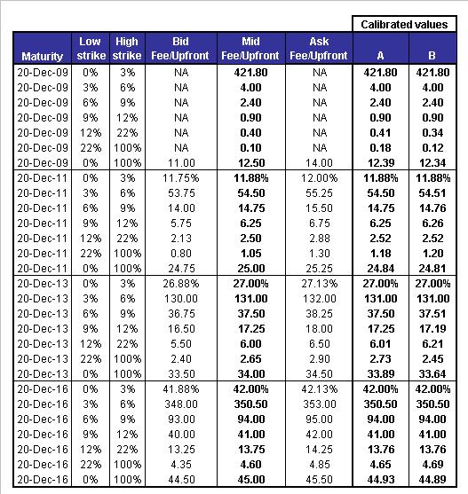
Figure 1: Calibration results for BSLP. Note that quotes are given as spreads in bps except for the 5,7, and 10y equity tranches which are quoted as upfront in percent (with a coupon of 500bps). Calibration is done to mid quotes. Indicative bid/ask quotes are included for reference to assess calibration quality. Note that 3y bid/ask spreads are not available.

5.2 Pricing

5.2.1 Tranchlets

Next we investigate the behavior of the two calibrated BSLP models A and B. First we look at implied tranchlet pricing, i.e. prices of thin CDO tranches on the iTraxx portfolio. In particular we look at the 10 year $1\%$-wide tranches up to $12\%$ and plot the results in Fig. 2.

The first observation is that the tranchlet curve is close to linear on a logarithmic scale, resulting in a smooth interpolation and extrapolation to the equity region.

The second observation is that the $0\%$ and $75\%$ volatility cases produce nearly identical curves. This is a reassuring result that suggests that the local intensity model is indeed sufficient for tranche price interpolation. Note that this is not a completely trivial observation. Indeed, similarly to regular tranches, tranchlet prices are determined by a set of marginal loss distributions at a set of horizons. However, market tranche quotes do not uniquely define those marginal probabilities; they only provide integral constraints on them (i.e. the market is incomplete - see also the remarks at the end of section 3.6). When we calibrate BSLP with volatilities $0\%$ and $75\%$, strictly speaking we end up with two different sets of marginal loss distributions, whose difference could in principle amplify when projected onto thin tranchlets. Thus our findings imply that volatility assumptions have a negligible impact on marginal loss distributions even for incomplete markets.

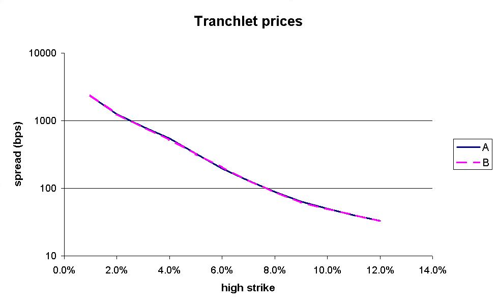
Figure 2: Tranchlet ($1\%$-wide) prices for models A and B on logarithmic scale. Maturity is the 20th December 2016.

5.2.2 Tranche Options

The main aim of the BSLP model is to price exotic credit derivatives. Here we look at the tranche option as an example. We focus on 5y into 5y options, i.e. exercise date 20-Dec-2011 and maturity 20-Dec-2016. The tranches we consider here are the index ($0\%-100\%$) and the equity ($0\%-3\%$) tranche.

Figs. 3 and 4 show the implied (Black) volatilities for these options for both model choices A and B.

We start by discussing the index option (Fig. (3)). It can be seen clearly that for both models A and B there is a strong skew in the implied volatilities.

It should be noted that even for model A which has $0\%$ volatility for the portfolio intensity the implied volatilities are high (the ATM vol is around $22\%$). As we will see in the next section, this is because the model gives rise to a non-zero dispersion of forward spreads even in the absence of Y-volatility.

One can also see that adding non-zero $Y$-volatility results in a rotation of the volatility smile curve, i.e. volatilities increase for low strikes and decrease for high strikes. Again, this can be understood by looking at the behavior of the conditional forward spreads as discussed in section 5.2.3.

For the equity option (Fig. (4)) we note that increasing $Y$-volatility results in an upward parallel shift of the smile curve. We can also see that the curve for the local intensity model (A) is not very smooth. This is a result of the fact that the local intensity model is fundamentally discrete, i.e. the dynamic default variable can only take on integer values. This means in turn that the distribution of conditional forwards is also discrete. As a result option prices are linear for strikes that lie between the conditional forward levels.

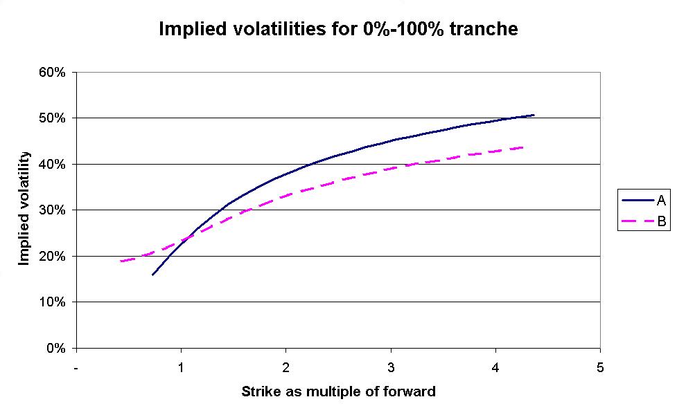
Figure 3: Implied volatilities for index ($0\%-100\%$ tranche) option. Exercise date is 20-Dec-2011 and maturity is 20-Dec-2016. Strikes are given as a multiple of the forward value, which is at 69bps.

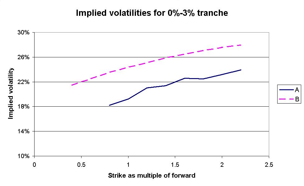
Figure 4: Implied volatilities for equity ($0\%-3\%$ tranche) option. Exercise date is 20-Dec-2011 and maturity is 20-Dec-2016. Strikes are given as a multiple of the forward value, which is at 2725bps.

5.2.3 Conditional Forwards

A key quantity for assessing dynamics of a multi-period model is the forward spread distribution. Here we focus on the 5 year spreads, conditional on the default level at 20-Dec-2011.

These spreads tell us how the model links spread and default dynamics. This can be compared to intuition on how risk will be priced in different (default) states of the world. Of course these forwards will also play a direct role in exotic pricing, e.g. a tranche option can be viewed as essentially an option on the forward spread.

The forwards levels are plotted in Figs. 5 and 6 for  $0\%-100\%$ and a $3\%-6\%$ tranche respectively.

First we should note that $0\%$ volatility (model A) does not imply 0 variance for the distribution of conditional forwards. This leads to non-zero implied tranche option volatilities as described in the previous section. The reason for this is that even though there is no spread diffusion, we still have spread jumps determined by the contagion factors.

One can also see a rapid increase in spread levels as defaults increase, which indicates that the model implies a high level of contagion. An interesting feature is that the increase in forward spreads is less pronounced for model B than A, i.e. introducing $Y$-volatility reduces the level of contagion.

This can be understood since we are replacing spread contagion with spread diffusion while calibrating to the same portfolio loss distribution. Another way to see this is to note that adding spread diffusion will decorrelate losses and spreads.

This is an important effect, which is likely to have significant impact on exotic pricing.

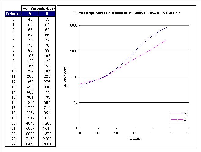
Figure 5: Forward spreads on a logarithmic scale conditional on the default level for the index tranche for models A and B. Start date is 20-Dec-2011 and maturity is 20-Dec-2016. The unconditional forward level is ca. 69bps.

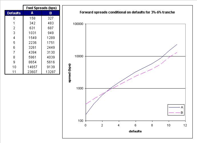
Figure 6: Forward spreads on a logarithmic scale conditional on the default level for $3\%-6\%$ tranche for models A and B. Start date is 20-Dec-2011 and maturity is 20-Dec-2016. The unconditional forward level is 750bps. Note that the tranche is wiped out after 11 defaults.

5.3 Risk

In this section we explore the first order (spread) risk in the BSLP model. Since BSLP is driven by a stochastic $Y$-process, it is natural to look at deltas with respect to moves in todays value $Y_{0}$. The meaning of this procedure can be clarified using Eq.(31): if we keep contagion factors $F(N_{k},0)$ constant and shift $Y_{0}$, this is equivalent to shifting the index swap intensity $\lambda_{s}(0)$, and thus can be used to specify the index delta.

We note that, the same Eq.(31) also shows that shifting $Y_{0}$ while keeping contagion factors $F(N_{k},0)$ constant is equivalent to a common rescaling of all contagion factors.

5.3.1 Tranche Deltas

First we look at how tranche prices behave as we shift the initial $Y$-value, $Y_{0}$. In particular, we can look at the hedge ratio to the index.

Let us denote the mark-to-market of a tranche with low strike $k$, high strike $l$ and coupon $c$ as a function of $Y_{0}$ by: $\mathcal{M}_{[k,l]}(c,Y_{0})$. The par spread of this tranche is $S_{[k,l]}$, defined by:

$$\mathcal{M}_{[k,l]}(S_{[k,l]},Y_{0})=0$$ (74)

For a given tranche with strikes $k$ and $l$, we now define the tranche delta $\Delta_{[k,l]}$ as follows:

$$\Delta_{[k,l]}\equiv\frac{\mathcal{M}_{[k,l]}(S_{[k,l]},Y_{0}+\epsilon)-\mathcal{M}_{[k,l]}(S_{[k,l]},Y_{0})}{\mathcal{M}_{[0,1]}(S_{[0,1]},Y_{0}+\epsilon)-\mathcal{M}_{[0,1]}(S_{[0,1]},Y_{0})}=\frac{\mathcal{M}_{[k,l]}(S_{[k,l]},Y_{0}+\epsilon)}{\mathcal{M}_{[0,1]}(S_{[0,1]},Y_{0}+\epsilon)}$$ (75)

For index tranches these deltas can be compared to the quoted spread deltas. This is done in Fig. 7. We see that deltas are reasonably close to the quoted values. BSLP deltas tend to be lower in the equity region and higher for super senior tranches. We note also that adding $Y$-volatility (model B) tends to improve the delta match.

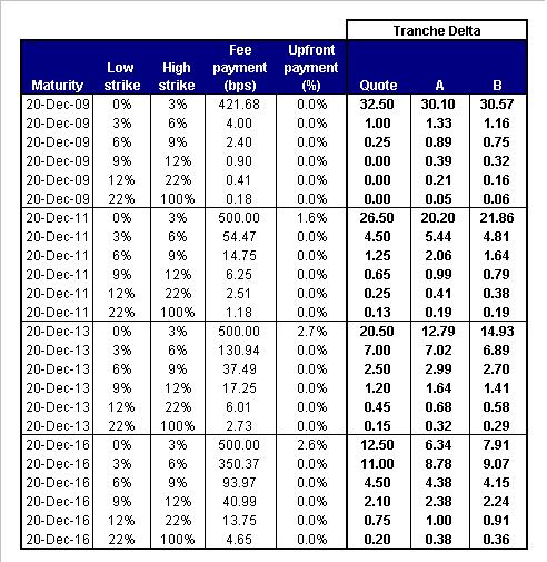
Figure 7: Tranche deltas computed with models A and B compared to iTraxx quoted deltas.

5.3.2 Option Deltas

We now look at deltas of tranche options. Again we consider the impact of a shift in initial $Y$-level and compute the option delta as the change in mark-to-market of the option divided by the change in mark-to-market of the forward tranche. In other words we are computing the hedge ratio of the tranche option with respect to a position in the underlying forward.

We can compare this to the hedge ratio obtained by using the Black formula. In this case we first calculate the implied Black volatility of the option. After shifting $Y_{0}$ we get new forward levels and risky annuities for the underlying tranche. Using these shifted forwards and annuities but keeping the implied volatility constant we can compute a new option price using the Black formula. This gives rise to a Black delta or hedge ratio.

The results are given for a $0\%-3\%$ equity tranche option and the $0\%-100\%$ index option in Figs. 9 and 8 respectively. As before the exercise date of the options is 20-Dec-2011 and the maturity is 20-Dec-2016.

We can see that BSLP and Black deltas are of the same order. The match is better for the equity option than the index option, especially for high strikes. We note also that Black and BSLP deltas are closer to each other for model specification B, i.e. with non-zero $Y$-volatility.

As in the case of the implied Black volatility smile we can see that the curve of option deltas as a function of strike is not very smooth for the $0\%$ volatility case. Again this is due to the fundamental discreteness of the local intensity model.

Figure 8: Option deltas for the index tranche computed with models A and B compared to Black option deltas. Strikes are given as multiples of the forward level which is ca. 69bps.

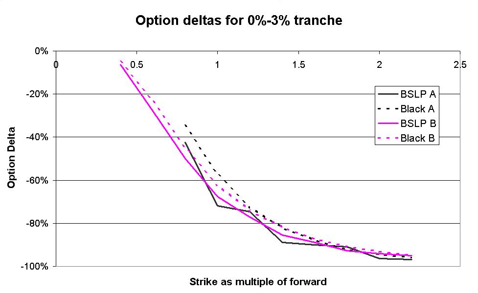
Figure 9: Option deltas for the $0\%-3\%$ equity tranche computed with models A and B compared to Black option deltas. Strikes are given as multiples of the forward level which is ca. 2725bps.

6 Summary

BSLP is a model of the portfolio loss and loss intensity. It can be used for the pricing and risk management of vanilla as well exotic credit derivatives which depend on the portfolio loss.

Because the model is low-dimensional and Markovian, efficient lattice or tree implementations are possible. In addition to such numerical methods, analytical approaches such as the adiabatic approximation can be used. A possible extension to the model considers multi-factor generalizations of the driving stochastic process.

BSLP explicitly models credit contagion and provides insight on how this impacts the forward loss dynamics. This is a key for the pricing and risk management of exotic portfolio credit derivatives.

The model achieves a near perfect calibration to any set of portfolio tranche quotes due to a semi-parametric representation of the contagion factors. These quotes can either be obtained from the market for liquid indices or from an underlying bespoke tranche pricing model.

Efficient lattice or tree pricing algorithms for the model have been developed, including fast calibration algorithms based on a 1D projection of the full 2D model. Tree pricing is most suitable for pricing exotic credit portfolio derivatives that incorporate optionality and/or weak loss-path dependence such as tranche options, forward tranches, leveraged super-senior etc.. However, Monte Carlo implementations of the model (not discussed in this paper) are also possible in order to price more strongly path dependent products.

The calibrated model retains flexibility in adjusting the dynamics by choosing a concrete specification of the underlying stochastic driving process. This provides some freedom in the pricing of exotic derivatives. The local intensity limit of BSLP is a model in its own right that can be used to price non-standard tranches by arbitrage-free interpolation.

Appendix A: Swap intensity and NtD intensity

Here we formally derive the relation (31) between the NtD intensities specifying the transition probabilities (27) in the full 2D model, and the stochastic index swap intensity $\lambda_{s}(t)$.

The swap intensity is defined as the intensity that prices the index correctly as a single name CDS. More precisely, we want the following. Given a stochastic intensity $\lambda_{s}(t)$ we denote the distribution, $Q(t,T)$, of the first jump $\tau$ of the associated counting process by:

$$Q(t,T)\equiv P[\tau>T|\mathcal{F}_{t}]$$ (A.1)

This is all we need to price a CDS. To ensure that the value of this CDS corresponds to the value of the index calculated using the portfolio default process $N_{t}$ we need:

$$Q(t,T)=\frac{\mathbb{E}\left[N-N_{T}|\mathcal{F}_{t}\right]}{N-N_{t}}$$ (A.2)

The intensity corresponding to $Q(t,T)$ is given by:

$$\lambda_{s}(t)=-\left.\frac{\partial Q}{\partial T}\right|_{t}(t,T)$$ (A.3)

Using equation (A.2) this gives:

$$\lambda_{s}(t)dt=\frac{\mathbb{E}[N_{t+dt}|\mathcal{F}_{t}]-N_{t}}{N-N_{t}}$$ (A.4)

We can evaluate the conditional expectation in (A.4) as follows:

$$\mathbb{E}[N_{t+dt}|\mathcal{F}_{t}]=\sum_{k=0}^{N-N_{t}}(N_{t}+k)P[N_{t+dt}=N_{t}+k|N_{t},Y_{t},t]$$ (A.5)

where $P[N_{t+dt}=N_{t}+k|N_{t},Y_{t},t]$ is the probability of the transition $N_{t}\rightarrow N_{t+dt}=N_{t}+k$. As we only allow for at most one step transition in the infinitesimal time $dt$, the sum in (A.5) reduces to just two terms:

$$\mathbb{E}[N_{t+dt}|\mathcal{F}_{t}]=(N_{t}+1)\lambda_{NtD}(N_{t},Y_{t},t)dt+N_{t}\left(1-\lambda_{NtD}(N_{t},Y_{t},t)dt\right)$$ (A.6)

Substituting this relation into (A.4), we arrive at the sought-after relation between the two intensities:

$$\lambda_{s}(N_{t},Y_{t},t)=\frac{\lambda_{NtD}(N_{t},Y_{t},t)}{N-N_{t}}$$ (A.7)

Note that $\lambda_{s}(t)$ is also the average of the portfolio single name intensities $\lambda_{i}$. This follows since in the absence of simultaneous defaults we know that the portfolio default intensity $\lambda_{NtD}$ is just given by the sum of single name intensities. In other words:

$$\lambda_{NtD}=\sum_{i=1}^{N-N_{t}}\lambda_{i}=(N-N_{t})\lambda_{s}$$ (A.8)

Appendix B: BSLP in continuous time

Here we present a continuous-time formulation of the BSLP model for a jump-diffusion specification of the driving $Y$-process given in Eq.(28). (A continuous-time formulation with a discretized $Y$-variable is further analysed in Appendix C). In this appendix, we will use a more conventional notation $(x,y)$ instead of $(N,Y)$ for the dynamic variables of the BSLP model, with $x$ denoting the defaulted fraction $N_{t}/N$ instead of the absolute default level $N_{t}$.

The general form of the infinitesimal jump-diffusion generator $\mathcal{L}$ acting on the pdf $P(\vec{z}^{\prime},t|\vec{z},s)$ for $n$-dimensional random variables $\vec{z}^{\prime},\,\vec{z}\in R^{n}$ is as follows

$$\mathcal{L}P(\vec{z}^{\prime},t|\vec{z},s) = \sum_{i=1}^{n}\mu_{i}(\vec{z},s)\frac{\partial P(\vec{z}^{\prime},t|\vec{z},s)}{\partial z_{i}}+\sum_{i,j=1}^{n}\frac{1}{2}\sigma_{ij}^{2}(\vec{z},s)\frac{\partial^{2}P(\vec{z}^{\prime},t|\vec{z},s)}{\partial z_{i}\partial z_{j}}$$ (B.1)

$$+ \sum_{\vec{z}^{\prime\prime}\neq\vec{z}}W(\vec{z}^{\prime\prime}|\vec{z},s)\left[P(\vec{z}^{\prime},t|\vec{z}^{\prime\prime},s)-P(\vec{z}^{\prime},t|\vec{z},s)\right]$$

while the adjoint operator $\mathcal{L}^{*}$ reads

$$\mathcal{L}^{*}P(\vec{z}^{\prime},t|\vec{z},s) = -\sum_{i=1}^{n}\frac{\partial}{\partial z_{i}^{\prime}}\left[\mu_{i}(\vec{z}^{\prime},t)P(\vec{z}^{\prime},t|\vec{z},s)\right]+\sum_{i,j=1}^{n}\frac{1}{2}\frac{\partial^{2}}{\partial z_{i}^{\prime}\partial z_{i}^{\prime}}\left[\sigma_{ij}^{2}(\vec{z}^{\prime},t)P(\vec{z}^{\prime},t|\vec{z},s)\right]$$ (B.2)

$$+ \sum_{\vec{z}^{\prime\prime}\neq\vec{z}}\left[W(\vec{z}^{\prime}|\vec{z}^{\prime\prime},t)P(\vec{z}^{\prime\prime},t|\vec{z},s)-W(\vec{z}^{\prime\prime}|\vec{z}^{\prime},t)P(\vec{z}^{\prime},t|\vec{z},s)\right]$$

Here $W(\vec{z}^{\prime}|\vec{z},t)$ is the jump measure determining the jump probability in time $dt$ together with the jump size distribution. Using standard conventions, we write

$$W(\vec{z}^{\prime}|\vec{z},t)=\lambda(\vec{z},t)w(\vec{z}^{\prime}-\vec{z}|\vec{z},t)$$ (B.3)

where $\lambda(\vec{z},t)$ stands for the jump rate (intensity) and $w(\delta\vec{z}|\vec{z},t)$ is a pdf of the jump size $\delta\vec{z}$ given the initial point $\vec{z}$. The forward and backward equations are

$$\frac{\partial P(\vec{z}^{\prime},t|\vec{z},s)}{\partial t}=\mathcal{L}^{*}P(\vec{z}^{\prime},t|\vec{z},s)\;\;,\;\;\frac{\partial P(\vec{z}^{\prime},t|\vec{z},s)}{\partial s}=-\mathcal{L}P(\vec{z}^{\prime},t|\vec{z},s)$$ (B.4)

We note that the generator can be written in the following form

$$A=\mathcal{L}_{0}+\mathcal{L}_{1}$$ (B.5)

where $\mathcal{L}_{0}$ and $\mathcal{L}_{1}$ correspond to diffusion and jump parts of the generator, given by the first two terms and the last term in (B.1), respectively.

Let us now define the operators $\mathcal{L}_{0}$ and $\mathcal{L}_{1}$ in our specific 2D setting with $\vec{z}=(x,y)$. In the BSLP model, the generator $\mathcal{L}_{0}$ acts only on $y$. We therefore set

$$\mathcal{L}_{0}P(x,y,t|x_{0},y_{0},s)=\mu(y_{0},s)\frac{\partial}{\partial y_{0}}P(x,y,t|x_{0},y_{0},s)+\frac{1}{2}\sigma^{2}(y_{0},s)\frac{\partial^{2}}{\partial y_{0}^{2}}P(x,y,t|x_{0},y_{0},s)$$ (B.6)

where the functions $\mu(y,t)$ and $\sigma(y,t)$ are defined in the SDE (28). For the adjoint operators we obtain

$$\mathcal{L}_{0}^{*}P(x,y,t|x_{0},y_{0},s)=-\frac{\partial}{\partial y}\left[\mu(y,t)P(x,y,t|x_{0},y_{0},s)\right]+\frac{1}{2}\frac{\partial^{2}}{\partial y^{2}}\left[\sigma^{2}(y,t)P(x,y,t|x_{0},y_{0},s)\right]$$ (B.7)

The second generator $\mathcal{L}_{1}$ corresponds to the case where jumps $x\rightarrow x+\Delta x$ are enabled, and in addition are accompanied by a related jump in $y$ (which arises due to the $dN_{t}$-term in (28)). The rate of this process is proportional to the product of the $y$-variable and the fraction of surviving names, times the contagion factor $F(x)=q(x)f(x)$, similarly to the treatment above:

$$\lambda(x,y,t)=y(1-x)q(x)f(x)$$ (B.8)

and the jump size distribution is a product of two delta-functions:

$$w_{1}(x-x_{0},y-y_{0}|x_{0},y_{0},s)=\delta(x-x_{0}-\Delta x)\delta(y-y_{0}-\Delta y)$$ (B.9)

Using (B.9) and (B.8), we calculate the generator $\mathcal{L}_{1}$

$$\mathcal{L}_{1}P(x,y,t|x_{0},y_{0},s) = \lambda(x_{0},y_{0},s)\left[P(x,y,t|x_{0}+\Delta x,y_{0}+\Delta y,s)\right.$$ (B.10)

$$- \left.P(x,y,t|x_{0},y_{0},s)\right]$$

and for the adjoint operator we have

$$\mathcal{L}_{1}^{*}P(x,y,t|x_{0},y_{0},s) = \lambda(x-\Delta x,y-\Delta y,t)P(x-\Delta x,y-\Delta y,t|x_{0},y_{0},s)$$ (B.11)

$$- \lambda(x,y,t)P(x,y,t|x_{0},y_{0},s)$$

To summarize, $\mathcal{L}_{0}$ in (B.5) collects terms in the generator $\mathcal{L}$ where $Y_{t}$ serves as the only dynamic variable while the default counting variable $N_{t}$ enters as a parameter. The second term $\mathcal{L}_{1}$ describes the part of the generator that contains both $Y_{t}$ and $N_{t}$ as dynamic variables. This special structure of the generator can be used to set up an adiabatic perturbation theory for the model (see Appendix D).

Appendix C: Discretized BSLP in continuous time

Here we discuss how the continuous-time formalism presented in Appendix B changes if we keep time continuous but assume that the $Y_{t}$-variable can only take discrete values from some finite set. Such analysis may be of interest as in this case the model becomes that of a 2D Markov chain, allowing powerful methods of Markov chain theory to be used to build fast and accurate numerical approximations to the dynamics of the original model, get more insight into the model behavior, and build connections to previous research. In particular, we will use this reformulation to compare our approach with the Davis-Lo model [12], as well as establish a link with a general and rich class of quasi-birth-death (QBD) processes.

Unlike the setting of Appendix B, which uses a jump-diffusion framework, here we assume that the $Y_{t}$-variable is discretized. For the general case of a two-dimensional process in the $NY$-plane, the states are parameterized by two indices $(i,n)$ ($i$ for number of defaults, and $n$ for $Y$-state). Correspondingly, the 2D generator carries four indices instead of two. We’ll use the notation $A_{in|jm}(t)$ for the matrix elements of the generator. In matrix notation, the generator can be viewed as a block matrix

$$A\,=\,\left(\begin{array}[]{clcrcc}L^{(0)}&F^{(0)}&0&0&\cdots&0\\ 0&L^{(1)}&F^{(1)}&0&\cdots&0\\ 0&0&L^{(2)}&F^{(2)}&\cdots&0\\ \vdots\\ 0&0&0&0&\cdots&0\end{array}\right)$$ (C.6)

where all matrices $L^{(i)},\,F^{(i)}$ have dimension $M\times M$, with $M$ being the dimension of the $Y$-space. The interpretation of these matrices is as follows. The matrix $L^{(i)}$ gives intensities of transitions between $Y$-states when there is no change of the $L$-state during the infinitesimal time step $\Delta t$, while the matrix $F^{(i)}$ provides intensities of joint events of a jump in the loss variable during the interval $[t,t+dt]$ accompanied by a transition between $Y$-states. As usual, all off-diagonal elements should be positive, diagonal elements should be negative, and each row in $A$ should sum up to zero.

Given the 2D generator matrix $A$, the forward equation takes a block-matrix form

$$\frac{\partial P(t,T)}{\partial T}=P(t,T)A$$ (C.7)

where $P(t,T)$ has matrix elements $P_{in|jm}(t,T)$.

The Davis-Lo model [12] is a particular case of a QBD credit process where the dynamics of $Y$ is locally deterministic. Matrix elements of $A$ are given in this model by $2\times 2$ matrices

$$L^{(i)}=\,\left(\begin{array}[]{cc}-\lambda(N-i)&0\\ \mu&-\mu-a\lambda(N-i)\end{array}\right)\;\;F^{(i)}=\,\left(\begin{array}[]{cc}0&\lambda(N-i)\\ 0&a\lambda(N-i)\end{array}\right)$$ (C.12)

Note that the form of $F^{(i)}$ implies that whenever there is a default in a given time step $dt$, the probability for the hidden variable $Y$ to stay in state “0” is zero, meaning it jumps to state “1” (“risky state”) with (conditional) probability 1 , or stays in state “1” with (conditional) probability 1 if it was already there at the beginning of the time step. The matrix $L^{(i)}$ is interpreted similarly.

In the BSLP model, the dynamics of $Y$ is Markov as opposed to being locally deterministic (as in the Davis-Lo model), thus matrices $L^{(i)}$ and $F^{(i)}$ will have very few, if any, zero elements, as in general all transition probabilities between different $Y$-states will be non-vanishing. Note that the generator (C.6) can be identically re-written as follows:

$$A\,=\,\left(\begin{array}[]{clcrc}\tilde{L}^{(0)}&0&0&\cdots&0\\ 0&\tilde{L}^{(1)}&0&\cdots&0\\ 0&0&\tilde{L}^{(2)}&\cdots&0\\ \vdots\\ 0&0&0&\cdots&0\end{array}\right)+\left(\begin{array}[]{clcrc}-\tilde{F}^{(0)}&F^{(0)}&0&\cdots&0\\ 0&-\tilde{F}^{(1)}&F^{(1)}&\cdots&0\\ 0&0&-\tilde{F}^{(2)}&\cdots&0\\ \vdots\\ 0&0&0&\cdots&0\end{array}\right)\equiv A_{0}+A_{1}$$ (C.23)

where $\tilde{L}^{(i)}=L^{(i)}+\mbox{diag}\left(F^{(i)}\mathbb{I}\right)$, $\tilde{F}^{(i)}=\mbox{diag}\left(F^{(i)}\mathbb{I}\right)$. Both matrices $A_{0}$ and $A_{1}$ can be separately interpreted as generators, as in both of them off-diagonal elements are positive, diagonal ones are negative, and the row-wise sums are zeros. Note that they have a straightforward interpretation: generator $A_{0}$ corresponds to the case when no $L$-transitions occur during the infinitesimal time step $dt$, while $A_{1}$ allows jumps in the $L$-process during the interval $[t,t+dt]$, that are accompanied by possible transitions between $Y$-states. Note that this decomposition is a discrete counterpart of (B.5).

Appendix D: Adiabatic approximation in the continuous time BSLP model

To get a tractable approximation to pricing index (or tranche) options, we assume that the characteristic time scales of changes in $Y$ and $N$ ($\tau_{spread}$ and $\tau_{loss}$, respectively) are significantly different. We expect this approximation to yield accurate results because spreads change daily while loss states change very infrequently. To acknowledge the presence of a hidden small parameter $\sim\tau_{spread}/\tau_{loss}$ in the problem, we re-write the infinitesimal generator (B.5) of the BSLP model as follows:

$$A=\frac{1}{\varepsilon}\mathcal{L}_{0}+\mathcal{L}_{1}$$ (D.1)

where the parameter $\varepsilon>0$ is assumed to be small. Matrices $\mathcal{L}_{0}/\varepsilon$ and $\mathcal{L}_{1}$ correspond to parts of the generator responsible for the $y$-dependent part (where the default counting variable $N_{t}$ may enter as a parameter) $A_{0}$ and a second term $A_{1}$ that contains both $N_{t}$ and $Y_{t}$ as dynamic variables. In particular, for the OU specification (3.1) with mean reversion parameter $a=1/\varepsilon$ and variance $\nu^{2}=\sigma^{2}/(2a)$, we obtain

$$\mathcal{L}_{0}=(\theta-y_{0})\frac{\partial}{\partial y_{0}}+\nu^{2}\frac{\partial^{2}}{\partial y_{0}^{2}}$$ (D.2)

Given these assumptions, we consider the adiabatic approximation (see e.g. [16] for financial applications of this method) to find the forward and backward dynamics in the form of asymptotic series in powers of $\varepsilon$. We restrict ourselves to a calculation of the leading order adiabatic approximation for the backward equation.

Consider the backward equation for some function $B(x,t)$ of initial values $(x,t)$ (this function can be a conditional expectation or a transition probability viewed as a function of the initial variables):

$$\frac{\partial B}{\partial t}=-\mathcal{L}B=-\left(\frac{1}{\varepsilon}\mathcal{L}_{0}+\mathcal{L}_{1}\right)B$$ (D.3)

We look for a solution in the form

$$B=B_{0}+\varepsilon B_{1}+\varepsilon^{2}B_{2}+\ldots$$ (D.4)

Plugging this into (D.3) and equating like powers of $\varepsilon$, we obtain the chain of equations

$$\mathcal{L}_{0}B_{0} = 0$$

$$\mathcal{L}_{0}B_{1} = -\frac{\partial B_{0}}{\partial t}-\mathcal{L}_{1}B_{0}$$ (D.5)

$$\mathcal{L}_{0}B_{2} = -\frac{\partial B_{1}}{\partial t}-\mathcal{L}_{1}B_{1}$$

As the generator $\mathcal{L}_{0}$ depends only on $y$, the solution to the first equation is

$$B_{0}=B_{0}(x,t)$$ (D.6)

i.e. a function (unknown at this stage) of $x$ and $t$ only. To find this function, we multiply both sides of the second equation in (Appendix D: Adiabatic approximation in the continuous time BSLP model) by the stationary state $\rho_{0}(y,x)$ of the adjoint generator $\mathcal{L}_{0}^{*}$, i.e. $\mathcal{L}_{0}^{*}\rho_{0}(y,x)=0$. The left hand side of this equation vanishes, hence the right hand side should vanish as well. This implies that $B_{0}(x,t)$ should solve the equation

$$0=\langle\frac{\partial B_{0}}{\partial t}+\mathcal{L}_{1}B_{0}\rangle=\frac{\partial B_{0}}{\partial t}+\langle\mathcal{L}_{1}\rangle B_{0}$$ (D.7)

where

$$\langle\mathcal{L}_{1}\rangle\equiv\int dy\rho_{0}(y,x)\mathcal{L}_{1}(y,x)$$ (D.8)

That is, $B_{0}(x,t)$ satisfies the backward equation in the $L$-space where the fast $Y$-dynamics is integrated out in the generator $\mathcal{L}_{1}$ with weight equal to the invariant distribution $\rho_{0}(y,x)$ of $\mathcal{L}_{0}^{*}$. Correction terms $B_{1},\,B_{2},\ldots$ can be found from further equations in (Appendix D: Adiabatic approximation in the continuous time BSLP model).

Let us consider the leading order adiabatic approximation formulas. Using (D.7) and (B.10), we obtain the following equation for the lowest order term $B_{0}(x,t)$:

$$\frac{\partial B_{0}}{\partial t}=-\bar{\lambda}(x)\left(B_{0}(x+\Delta x,t)-B_{0}(x,t)\right)$$ (D.9)

where

$$\bar{\lambda}(x)\equiv(1-x)q(x)f(x)\langle y\rangle=(1-x)q(x)f(x)\int dy\,y\rho_{0}(y,x)$$ (D.10)

Thus to the leading order in the adiabatic approximation, we find that the backward dynamics can be described as the 1D pure default dynamics with a rescaled intensity. If we further impose the condition that the intensity of this effective 1D model should be equal to the intensity $(1-x)\lambda f(x)$ of the original default-only model, we obtain the following expression for the drift adjustment factor $q(x)$:

$$q(x)=\frac{\lambda}{\langle y\rangle_{x}}=\frac{\lambda}{\int y\rho_{0}(y,x)dy}$$ (D.11)

One notes a similarity between(D.11) and (57). The difference between them is that while (57) contains the full time-dependent distrubution $\pi(Y_{t},t|N_{t})$, it is the steady state distribution $\rho_{0}(y,x)=\lim_{t\rightarrow\infty}\pi(Y_{t},t|N_{t})$ that appears in (D.11).

Corrections to the zero-order result $B_{0}=B_{0}(x,t)$ can now be found from equations (Appendix D: Adiabatic approximation in the continuous time BSLP model). In particular, after the right hand side of the second equation in (Appendix D: Adiabatic approximation in the continuous time BSLP model) is “centered” (i.e. its expectation is zeroed by the choice of $B_{0}$), we can write this equation as follows:

$$\mathcal{L}_{0}B_{1}=\left(\langle\mathcal{L}_{1}\rangle-\mathcal{L}_{1}\right)B_{0}$$ (D.12)

This is the so-called Poisson equation that can be explicitly solved to find the first correction $B_{1}$, as described in [16].

Information has been obtained from sources believed to be reliable but JPMorgan Chase & Co. or its affiliates and/or subsidiaries (collectively JPMorgan) does not warrant its completeness or accuracy. Opinions and estimates constitute our judgement as of the date of this material and are subject to change without notice. Past performance is not indicative of future results. This material is not intended as an offer or solicitation for the purchase or sale of any financial instrument. Securities, financial instruments or strategies mentioned herein may not be suitable for all investors. The opinions and recommendations herein do not take into account individual client circumstances, objectives, or needs and are not intended as recommendations of particular securities, financial instruments or strategies to particular clients. The recipient of this presentation must make its own independent decisions regarding any securities or financial instruments mentioned herein. JPMorgan may act as market maker or trade on a principal basis, or have undertaken or may undertake account transactions in the financial instruments or related instruments of any issuer discussed herein and may act as underwriter, placement agent, advisor or lender to such issuer. JPMorgan and/or its employees may hold a position in any securities or financial instruments mentioned herein. Important disclosures are available on a company specific basis at http://mm.jpmorgan.com/disclosures/company. Additional information available upon request.

References

- [1] K. Giesecke and L. Goldberg, “ A Top Down Approach to Multi-Name Credit”, working papers (2005).
- [2] P. Schönbucher, “Portfolio Losses and the Term Structure of Loss Transition Rates”, working paper (2005).
- [3] J. Sidenius, V. Piterbarg, and L. Andersen, “A New Framework for Dynamic Credit Portfolio Modelling”, working paper (2005).
- [4] N. Bennani, “The Forward Loss Model: a Dynamic Term Structure Approach for the Pricing of Portfolio Credit Derivatives”, working paper (2005) available at www.defaultrisk.com.
- [5] D. Brigo, A. Pallavicini, and R. Torresetti, “Calibration of CDO Tranches with the Dynamical Generalized-Poisson Loss Model”, working paper (2006), available at www.defaultrisk.com.
- [6] A. Chapovsky, A. Rennie, and P.A.C. Tavares, “Stochastic Intensity Modelling for Structured Credit Exotics”, working paper (2006), available at www.defaultrisk.com
- [7] E. Errais, K. Giesecke and L. Goldberg, “Pricing Credit from the Top Down with Affine Point Processes”, working paper (2006).
- [8] R. Cont and I. Savescu, “Forward Loss Models for Portfolio Credit Derivatives”, presented at Credit Risk Summit, New York, Oct. 2006.
- [9] X. Ding, K. Giesecke, and P. Tomocek, “Time-Changed Birth Processes and Multi-Name Credit”, working paper (2006), available at www.defaultrisk.com.
- [10] J. de Kock, H. Kraft, and M. Steffensen, “CDO in Chains”, working paper (2007), available at www.defaultrisk.com.
- [11] A.V. Lopatin and T. Misirpashaev, “Two-Dimensional Markovian Model for Dynamics of Aggregate Credit Loss”, working paper (2007), available at www.defaultrisk.com.
- [12] M. Davis and V. Lo, “Modelling Default Correlation in Bond Portfolio” (2001).
- [13] R. Frey and J. Backhaus, “Credit Derivatives in Models with Interacting Default Intensities: a Markovian approach” (2006), available at www.defaultrisk.com.
- [14] M. Britten-Jones and A. Neuberger, “Option Prices, Implied Price Processes, and Stochastic Volatility”, Journal of Finance, 55 (2000), p. 839.
- [15] W. Feller, “An Introduction to Probability Theory and its Applications” , Wiley 1957.
- [16] J.P. Fouque, G. Papanicolaou and K.R. Sircar, “Derivatives in Financial Markets with Stochastic Volatility”, Cambridge University Press (2000).