Marangoni shocks in unobstructed soap-film flows

Abstract

It is widely thought that in steady, gravity-driven, unobstructed soap-film flows, the velocity increases monotonically downstream. Here we show experimentally that the velocity increases, peaks, drops abruptly, then lessens gradually downstream. We argue theoretically and verify experimentally that the abrupt drop in velocity corresponds to a Marangoni shock, a type of shock related to the elasticity of the film. Marangoni shocks induce locally intense turbulent fluctuations and may help elucidate the mechanisms that produce two-dimensional turbulence away from boundaries.

Soap-film flows soapf have long been used to study two-dimensional (2-D) turbulence, a type of turbulence that differs from its three-dimensional (3-D) counterpart in crucial respects. For example, in 3-D turbulence the energy may cascade only from larger to smaller lengthscales whereas in 2-D turbulence the energy may cascade in either direction cascade . Disparate directions of energy transfer result in disparate apportionings of the turbulent kinetic energy among the lengthscales of the flow cascade . Besides the theoretical interest inherent in its distinctive characteristics, 2-D turbulence is relevant to the large-scale irregularities encountered in 2-D atmospheric flows—flows that are confined to two dimensions by geostrophic forces and a stratified atmosphere twod . Examples of large-scale irregularities in 2-D atmospheric flows include hurricanes, typhoons, and the Great Red Spot of Jupiter atmo .

In the typical setup used to study soap-film flows rutgers2001 , a film hangs between two long, vertical, mutually parallel wires a few centimeters apart from one another. Driven by gravity, a steady vertical flow soon becomes established within the film (Fig. 1). Then, the thickness $h$ of the film is roughly uniform on any cross section of the flow georgiev2002 , and we write $h=h(x)$, where $x$ runs along the centerline of the flow (Fig. 1). In a typical flow $h\approx 10\,\mu$m, much smaller than both the width $w$ and the length $L$ of the flow (Fig. 1). As a result, the velocity of the flow lies on the plane of the film, and the flow is 2-D. Since the viscous stresses (and the attendant velocity gradients) are confined close to the wires, the mean (time-averaged) velocity $u$ is roughly uniform on any cross section of the film rutgers1996 , and we write $u=u(x)$. Thus, assuming incompressibility, $h(x)u(x)$ equals the flux $q$ per unit width of film and is independent of $x$ for a steady flow.

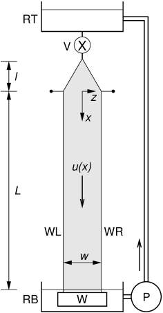
Figure 1: Typical setup used to study steady, gravity-driven, unobstructed soap-film flows. Axis $x$ runs vertically along the centerline of the flow. Wires WL and WR are thin nylon-fishing lines kept taut by weight W. The film hangs from the wires; its width increases from 0 to $w$ over an expansion section of length $l$, then remains constant and equal to $w$ over a measurement section of length $L\gg l$. (The origin of $x$ is at the top of the measurement section. $L$ is the “length of the flow” and $w$ the “width of the flow.”) Reservoir RT contains a soapy solution which flows through valve V and into the film. After flowing through the film with mean velocity $u(x)$, the soapy solution drains into reservoir RB and returns to reservoir RT via pump P. In our experiments, the soapy solution consists of $\simeq 2.5\,$% Dawn Nonultra in water; $w=2.5$ to 5.1 cm; $L=1.05$ to 1.39 m; and $l=23.5\,$cm.

Analyses of steady flows have accounted for the gravitational force, the inertial force, the drag force of the ambient air, and the drag force of the wires. Rutgers et al.  rutgers1996 have shown that the drag force of the wires is negligible as compared to the drag force of the ambient air and may be dropped from the equation of momentum balance. Then, a prediction can be made that in a steady flow the mean velocity is a monotonically increasing function of $x$ and approaches a terminal velocity asymptotically downstream rutgers1996 ; georgiev2002 . This prediction has not been tested, but it is thought to be in qualitative agreement with the few known experiments rutgers1996 ; georgiev2002 . In contrast to this prediction, in our experiments $u(x)$ is a strongly non-monotonic function of $x$.

To measure $u$, we use laser Doppler velocimetry (LDV). In Fig. 2 we show plots of $u$ along the centerline of several representative flows. In each flow, $u$ increases downstream up to a certain point whereupon it peaks, drops abruptly to a fraction of its peak value, then continues to lessen gradually downstream.

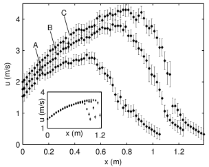
Figure 2: Plots of the mean velocity $u$ vs. $x$ for three steady flows. The width $w=5.1\,$cm for all flows; both the length $L$ and the flux per unit width $q$ change from flow to flow. $L=1.05\,$m and $q=3.8\,10^{-6}\,$m²/s (A), $L=1.23\,$m and $q=4.9\,10^{-6}\,$m²/s (B), $L=1.39\,$m and $q=5.5\,10^{-6}\,$m²/s (C). Inset: Plots of $u$ vs. $x$ for three steady flows. $w=5.1\,$cm and $q=5.7\,10^{-6}\,$m²/s for all flows; $L$ changes from flow to flow.

From the incompressibility condition ($uh=q$), the abrupt drop in $u$ should be accompanied by an abrupt increase in $h$. To verify this abrupt increase in $h$, we light one face of a film with a sodium lamp and observe the interference fringes that form there. In Fig. 3a we show a photograph of the interference fringes on the part of a film where $u$ drops abruptly. The distance between successive fringes decreases rapidly in the downstream direction, signaling an abrupt increase in $h$.

To verify the abrupt increase in $h$ by means of an alternative technique, we put Flourescein dye in the soapy solution and focus incoherent blue light on a spot on the film. The spot becomes fluorescent, and we monitor the intensity of the fluorescence using a photodetector whose counting rate is proportional to $h$. In Fig. 3b we show plots of $h$ along four cross sections of a flow. These cross sections lie on the part of the flow where $u$ drops abruptly. The thickness trebles over a short distance of a few centimeters in the downstream direction.

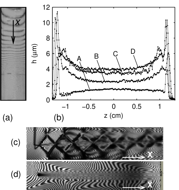
Figure 3: (a) Fringes over the part of a film where the velocity drops abruptly. (b) Plots of the thickness vs. $z$ along four cross sections of a flow of width $2.5\,$cm and length $1.2\,$m. The cross sections are at $x=0.95\,$m (A), $x=1.04\,$m (B), $x=1.05\,$m (C), and $x=1.07\,$m (D). The large peaks near the lateral edges are due to backscattering from the wires. Fringes at a piercing upstream (c) and downstream (d) of the drop in velocity; fields of view $=5\,$cm$\times 1\,$cm.

To explain our experimental results, we write the steady-state equation of momentum balance in the form

$$\rho huu_{x}=2\sigma_{x}+\rho gh-2\tau_{a},$$ (1)

where $\rho$ is the density, $(\cdot)_{x}=d(\cdot)/dx$, $\sigma$ is the surface tension, $g$ is the gravitational acceleration, and $\tau_{a}$ is the shear stress due to air friction. From left to right, the terms in (1) represent the inertial force, the elastic force, the gravitational force, and the drag force of the ambient air. Here we follow Rutgers et al. rutgers1996 and use (as a rough approximation) $\tau_{a}=0.3\sqrt{\rho_{a}\mu_{a}u^{3}/(x+l)}$, the Blasius expression for the shear stress on a rigid plate that moves at a constant velocity $u$ through air of density $\rho_{a}=1.2\,$kg/m³ and viscosity $\mu_{a}=1.7\times 10^{-5}\,$kg/ms.

To obtain an expression for $\sigma_{x}$, we argue that the concentration of soap molecules in the bulk of the film remains constant in our experiments (because there is no time for diffusional exchange between the bulk and the faces of the film couder1989 ; maratimeNEW ). Then, the film is said to be in the Marangoni regime, and $2\sigma_{x}=-\rho U_{M}^{2}h_{x}$ mararegNEW , where $U_{M}$ is the Marangoni speed—a property of the film, independent of $h$, that quantifies the speed at which disturbances in $h$ travel on the plane of the film couder1989 ; mararegNEW . By substituting $2\sigma_{x}=-\rho U_{M}^{2}h_{x}$ and $h=q/u$ in (1), we obtain the governing equation

$$u_{x}=u\frac{g-2\tau_{a}u/\rho q}{u^{2}-U_{M}^{2}}.$$ (2)

In (2) we can distinguish two types of flow: a supercritical flow in which $u>U_{M}$ and $u_{x}>0$, and a subcritical flow in which $u<U_{M}$ and $u_{x}<0$. We conjecture that in our experiments the flow is supercritical upstream of the drop in velocity and subcritical downstream. Consistent with this conjecture, for any fixed $q$ the flow upstream of the drop in velocity remains invariant to changes in the length of the flow (inset of Fig. 2).

To confirm that flows are supercritical upstream of the drop in velocity and subcritical downstream, we use pins to pierce a flow upstream and downstream of the drop in velocity (Figs. 3c and d, respectively). Upstream of the drop in velocity the Mach angle $\approx 50^{o}$ (from Fig. 3c), and the local $u=1.83\,$m/s (from an LDV measurement); thus $U_{M}\approx\sin 50^{o}\times 1.83\,$m/s$=1.4\,$m/s in our experiments.

Let us test the governing equation (2) for one of our experiments. We adopt a value of $U_{M}$ and a value of $q$ and perform two computations. First, we integrate (2) downstream from $x=0$ with boundary condition $u(0)=u_{0}$, where $u_{0}$ is the velocity measured at $x=0$ in the experiment bcond . This first computation gives a function $u(x)$ that should fit the experiment upstream of the drop in velocity. Second, we integrate (2) upstream from $x=L$ with boundary condition $u(L)=u_{L}$, where $u_{L}$ is the velocity measured at $x=L$ in the experiment bcond . This second computation gives a function $u(x)$ that should fit the experiment downstream of the drop in velocity. We perform the same computations for each one of our experiments trying different values of $q$ and $U_{M}$, and choose the optimal values of $q$ and the optimal value of $U_{M}$—that is to say, the values of $q$ (one for each experiment) and the value of $U_{M}$ (the same for all experiments) that yield the best fits to the experiments (Fig. 4). The optimal value of $U_{M}$, $1.48\,$m/s, is in remarkable agreement with our estimate from Fig. 3c ($1.4\,$m/s). The optimal values of $q$ are in reasonable agreement with the experimental estimates for $q$ flux (caption to Fig. 4).

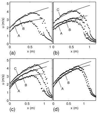
Figure 4: Plots of the computational $u(x)$ (lines) and experimental $u(x)$ (points) for ten different flows. The computations are for $U_{M}=1.48\,$m/s and the values of $q$ indicated below (the experimental estimates for $q$ are indicated in parentheses flux ). $w=5.1\,$cm for all flows. (a) Flows of length $1.05\,$m: (A) $q=5.7\,10^{-6}\,$m²/s ($3.9\,10^{-6}\,$m²/s), (B) $25\,10^{-6}\,$m²/s ($5.7\,10^{-6}\,$m²/s); (b) flows of length $1.17\,$m: (A) $5.7\,10^{-6}\,$m²/s ($5.1\,10^{-6}\,$m²/s), (B) $7.4\,10^{-6}\,$m²/s ($5.9\,10^{-6}\,$m²/s), (C) $30\,10^{-6}\,$m²/s ($7.5\,10^{-6}\,$m²/s); (c) flows of length $1.23\,$m: (A) $6.1\,10^{-6}\,$m²/s ($4.1\,10^{-6}\,$m²/s), (B) $14\,10^{-6}\,$m²/s ($5.3\,10^{-6}\,$m²/s), (C) $31\,10^{-6}\,$m²/s ($6.5\,10^{-6}\,$m²/s); and (d) flows of length $1.39\,$m: (A) $16\,10^{-6}\,$m²/s ($4.7\,10^{-6}\,$m²/s), (B) $25\,10^{-6}\,$m²/s ($6.3\,10^{-6}\,$m²/s).

We conclude that a drop in velocity signals a supercritical-to-subcritical transition and corresponds to a Marangoni shock. In theory the drop in velocity is infinitely steep and may be said to take place at $x=x^{*}$, where $u$ attains the value of $U_{M}$ (and $u_{x}$ becomes singular) in the subcritical flow (Fig. 4) theojump . But in experiments the drop in velocity takes place over a finite span $\Delta x$ whose magnitude appears to increase with $q$ (Fig. 4) and whose downstream edge is located at about $x=x^{*}$, the theoretical position of the shock (a position which appears to move downstream as $q$ increases). Thus in our simple theory the shock is sharp whereas in experiments the shock is diffused over a finite span $\Delta x$.

To understand the reason why our theory (which does not account for turbulence) cannot resolve the structure of the shock, recall that a shock must dissipate energy at a steady rate power . We argue (i) that the shock dissipates energy by powering locally intense turbulent fluctuations and (ii) that these fluctuations must extend roughly over the same span $\Delta x$ as the shock that powers them faber1997 .

To test these arguments we use LDV to measure the root-mean-square velocity $u_{\rm rms}$ along the centerline of a representative flow (Fig. 5). From a comparison of Figs. 5a and b, we confirm that the shock is accompanied over its entire span $\Delta x$ by velocity fluctuations that are up to thrice as intense as the velocity fluctuations that prevail both upstream and dowstream of $\Delta x$. We conjecture that intense velocity fluctuations can arise more readily where the mean velocity is higher; this may explain why the locally intense velocity fluctuations—and the diffusive shock that powers them—are located on the supercritical side of the theoretical position of the shock.

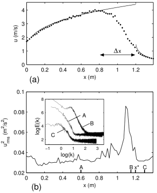
Figure 5: (a) Plots of the computational $u(x)$ (lines) and the experimental $u(x)$ (points) for a representative flow. $\Delta x$ is the span of the shock. (b) Plot of the experimental $u_{\rm rms}^{2}$ (an index of the energetic contents of the velocity fluctuations) vs. $x$ for the same flow. Inset: energy spectra at the centerline of the same flow for the cross section at $x=0.60\,$m (A), $x=1.17\,$m (B), and $x=1.30\,$m (C). These are the cross sections marked “A,” “B,” and “C” in part b. The spectra are log-log plots of the energy density $E$ (m³/s²) vs. the wavenumber $k$ (1/m).

To verify that the velocity fluctuations are turbulent, we obtain the energy spectrum on the centerline of the flow for three cross sections: one upstream, one within, and one downstream of the shock (inset to Fig. 5b). (These cross sections are marked “A,” “B,” and “C” in Fig. 5b.) The area under the spectrum is larger for cross section B than for cross sections A and C, confirming that the turbulence is more intense within the shock than elsewhere in the flow. Further, the slope of the spectrum at intermediate wavenumbers and the shape of the spectrum at low wavenumbers differ on either side of the shock, indicating that the spectrum undergoes structural changes as the flow traverses the shock.

We have demonstrated the spontaneous occurrence of shocks in the soap-film flows that are customarily used in experimental work on two-dimensional turbulence. These shocks are dissipative and diffusive; they give rise to fluctuations independently from the boundaries, with a strong but circumscribed effect on the spatial distribution of turbulent intensity; and they alter the structure of the turbulent spectrum downstream from the shock. We conclude that the presence of shocks should be factored in in the interpretation of experimental measurements, and submit that shocks may furnish a convenient setting to study localized turbulence production in two dimensions.

I Acknowledgements

NSF funded this reasearch through grants DMR06–04477 (UP) and DMR06–04435 (UIUC). The Vietnam Education Foundation funded T. Tran’s work. We thank Alisia Prescott, Jason Larkin, Nik Hartman, Hamid Kellay, Nicholas Guttenberg, and Nigel Goldenfeld.

References

- (1) M. Gharib and P. Derango, Physica D 37, 406 (1989); M. Beizaie and M. Gharib, Exp. Fluids 23, 130 (1997); H. Kellay and W. Goldburg, Rep. Prog. Phys. 65, 845 (2002); P. Tabeling, Phys. Rep. 362, 1 (2002).
- (2) R. Kraichnan, Phys. Fluids 10, 1417 (1967); G. Batchelor, ibid. 12, II-233 (1969); R. Kraichnan and D. Montgomery, Rep. Prog. Phys. 43, 547 (1980).
- (3) J. Pedlosky, Geophysical Fluid Dynamics (Springer-Verlag, 1987).
- (4) C. Leith, J. Atmos. Sci. 28, 145 (1971); C. Leith and R. Kraichnan, ibid. 29, 1041 (1972); M. Lesieur, Turbulence in Fluids (Kluwer Academic Publishers, Dordrecht, 1997); P. Marcus, Nature 428, 828 (2004); F. Seychelles et al., Phys. Rev. Lett. 100, 144501 (2008).
- (5) M. Rutgers, X. Wu and W.B. Daniel, Rev. Sci. Instrum. 72, 3025 (2001).
- (6) D. Georgiev and P. Vorobieff, Rev. Sci. Instrum. 73, 1177 (2002).
- (7) M. Rutgers et al., Phys. Fluids 8, 2847 (1996).
- (8) Y. Couder, J.M. Chomaz, and M. Rabaud, Physica D 37, 384 (1989); C.Y. Wen, S.K. Chang-Jian, and M.C. Chuang, Exp. Fluids 34, 173 (2003).
- (9) Note that a change in (and the attendant stretching of the film) may disturb the mutual equilibrium between the bulk and the faces of the film. To show that the concentration of soap molecules in the bulk remains constant, we must show that the rate of change of does not allow time for soap molecules to diffuse between the bulk and the faces of the film, so that (the timescale of diffusion) (the timescale associated with changes in ). For m (a typical value in our experiments) we estimate s couder1989 . To obtain an upper bound on , we argue that (the residence time of a drop of soapy solution in the flow) . For m/s and m (typical values in our experiments) we estimate , and conclude that .
- (10) The surface tension of a dilute soap solution can be expressed as , where is the surface tension of pure water, is the gas constant, is the absolute temperature, and is the concentration of soap molecules on the faces of the film couder1989 . Now, by definition , where is the overall concentration of soap molecules in the film and is the concentration of soap molecules in the bulk of the film. Since remains constant (because of incompressibility) and also remains constant (because the film is in the Marangoni regime), and , where is a constant independent of .
- (11) In actuality, we integrate downstream from with boundary condition , where is the velocity measured at in the experiment, and is the width of the flow (cm). Thus we avoid using the velocity measured at , where the flow is likely to be disturbed by end effects associated with the expanding section (Fig. 1). In an analogous way, we later integrate upstream from with boundary condition , where is the velocity measured at in the experiment.
- (12) We estimate these values of by measuring the volume of soapy solution that drains into reservoir RB (Fig. 1) in a given time interval and divide this volume by .
- (13) It may be argued theoretically that the sharp shock is located downstream of , where (Rayleigh’s jump condition, where and denote down and upstream of the jump, respectively.).
- (14) The energy per unit area on the plane of the film is the sum of the elastic, kinetic, and potential energy, . Thus the energy conveyed per unit time and unit width of film is , and the shock must dissipate a power per unit width , where . By substituting mararegNEW and , we obtain .
- (15) Here we argue by analogy with turbulent hydraulic jumps in open channels; see, e.g. T.E. Faber, Fluid Dynamics for Physicists (Cambridge U. Press, 1997) and D. Bonn, A. Anderson, and T. Bohr, J. Fluid Mech. 618, 71 (2009).