Identifying Multi-Top Events from Gluino Decay at the LHC
Abstract
We study the LHC signal of a light gluino whose cascade decay is dominated by channels involving top, and, sometimes, bottom quarks. This is a generic signature for a number of supersymmetry breaking scenarios considered recently, where the squarks are heavier than gauginos. Third generation final states generically dominate since third generation squarks are typically somewhat lighter in these models. At the LHC we demonstrate that early discovery is possible due to the existence of multi-lepton multi-bottom final states which have fairly low Standard Model background. We find that the best discovery channel is ’same sign dilepton’. The relative decay branching ratios into , and states carry important information about the underlying model. Although reconstruction will yield evidence for the existence of top quarks in the event, we demonstrate that identifying multiple top quarks suffers from low efficiency and large combinatorial background, due to the large number of final state particles. We propose a fitting method which takes advantage of excesses in a large number of channels. We demonstrate such a method will allow us to extract information about decay branching ratios with moderate integrated luminosities. In addition, the method also gives an upper bound on the gluino production cross section and an estimate of the gluino mass.
1 Introduction
Many considerations of new physics at the TeV scale point toward top rich final states at the LHC. Such scenarios include top compositeness [1], and models in which top partners ensure the naturalness of electroweak symmetry breaking [2, 3, 4, 5]. Compared with the Standard Model QCD production of , top quarks in the final states of new physics production typically either have very different kinematics [6, 7, 8], or different event topology [9, 11, 12, 10, 13], which may make it crucial to develop new techniques to identify them.
Naturalness of the electroweak symmetry breaking typically requires the existence of a light top partner. Experimental observations, ranging from the existence of Cold Dark Matter in the universe to the constraints of electroweak precision measurements, strongly motivates the existence of a neutral stable particle as particle of new physics signals at the LHC. The above considerations lead to the recent studies of new physics signals with final state [9].
In this article, we consider scenarios which also include a gluon partner, such as gluino in low energy supersymmetry [2, 14], the KK-gluon in universal extra dimension models [3], or other octet states [15, 16, 17]. Due to the nature of proton colliders, production of such color octet gluon partners and their decay typically becomes the main channel of new physics signals. Decay products of the gluon partner typically include an even number of quarks. Combining this with the scenario with light top partners, we conclude that a typical signature of production of gluon partners will be multiple top quarks in the final states.
In the rest of this paper, we will study this signature using a particular example, low energy supersymmetry with light gluinos. We will focus on the scenario in which the squarks are heavier than the gluino and the third generation squarks are lighter than those of the first two generations. In this case, the gluino will dominantly decay into top (bottom) quarks. Although not absolutely unavoidable, this is a generic possibility from the point of view of many models being studied recently [19, 18, 20, 21]. Heavier squark masses are often preferred due to constraints from flavor changing neutral currents [22, 23, 24]. RGE running of scalar masses from the high scale down to the electroweak scale will tend to push the third generation squark masses significantly lower than those of the other generations. Large third generation trilinear couplings will also help further lower one of the stop masses. For earlier studies on gluino decay into third generation quarks, see Refs. [25, 26, 27, 28, 29, 30, 31].
In the minimal case, this scenario has only a single, light top partner, . On the other hand, we would like to include in our study the possibility that all the squarks of the full third generation could be light relative to the other two generations. Therefore, we are led to consider decay channels , , and . As will be clear from our discussion later, many of the leading order features of the signature of different combinations of the above decay channels (from gluino pair production and decay) can be quite similar. Therefore, it is one of the primary purposes of this article to study techniques to distinguish them. We remark that such measurement is crucial for understanding both the spectrum of the third generation sfermions and the electroweak-inos. For example, if we measure a non-zero branching ratio for the decay channel , then there must be a light electroweak-ino carrying charge, suggesting that the lightest supersymmetric particle (LSP) is mostly Wino. Moreover, the relative branching ratio carries important information about the squark masses. For example, if this ratio is close to 1, it strongly suggests that left-handed squark masses are lighter than the right-handed ones, .
In section 3, we will focus on discovering new physics in this class of final states. Decay of multiple top quarks could lead to b-rich and lepton rich final states. Therefore, we expect great potential for early discovery. For example, we show that significant excesses can be observed in many channels even with just 500 pb-1 of data. The obvious channel with the best early discovery potential is same-sign dilepton plus additional b-tags.
In section 4, we study the problem of direct reconstruction of top quarks. Large combinatorics and high probability of object merging are expected due to the large multiplicity of final state particles. Therefore, while we may gather evidence from this study that there are some top quarks in the decay chain of the gluino, similar to the approaches taken in Ref. [26, 27, 15], the direct reconstruction efficiency for the top quark is low. We find that while the efficiency for reconstructing a single top quark candidate approaches , the efficiency to detect three and four candidates drops dramatically to and , respectively. As a result, it is less likely we can measure top multiplicity by direct reconstruction.
We will demonstrate in our study a fitting procedure which could allow us to measure the branching ratios of different gluino decay channels. We begin by simulating a number of samples of gluino pair production and decay, each with different final states, such as , , , and so on. Then we will fit the relative weights of different samples to match a set of experimental signatures. Of course, without precise knowledge of the underlying spectrum, choice of the templates will introduce errors in the estimate of the branching ratios. We studied such effects by using several templates with different hypotheses for the relevant masses. We conclude that such a method will allow us to establish important features of gluino branching ratios.
We carry out our study on several benchmark models with relatively low gluino masses. A detailed scan of the parameter space involving the gluino mass and different branching ratios is beyond the scope of this paper. The corresponding results for heavier gluino masses (but with similar decay branching ratio and mass difference between gluino and the LSP) could be roughly obtained by scaling from the present result using relative production cross sections. The mass gap between the gluino and the neutralino or chargino in the next step of the decay chain could also have important effects as it will affect the detection efficiency of various decay products. In general, a larger mass gap will enhance the discovery potential. At the same time, we expect this effect is milder in comparison with the dependence on the gluino mass.
We emphasize that our goal in this study is to demonstrate a method which allows us to extract information of the SUSY spectrum, such as the identity of the LSP with relatively low integrated luminosity. This is possible mainly because, unlike the precision measurements of the masses and couplings, our method mainly relies on inclusive counts and general kinematical features. Moreover, since we do not demand direct reconstruction, we are able to take advantage of many channels with multiple leptons. Due to lower background and theoretical uncertainty in comparison with the pure hadronic channel, we expect to have significant excesses in many of these channels. After discovery, we expect our method will yield a first set of clues about the underlying model during the early stages of LHC operation.
2 Benchmark Models
| Model parameters (TeV) | Branching ratios | |||||||||
|---|---|---|---|---|---|---|---|---|---|---|
| A | 0.65 | 0.1 | 0.92 | 0.07 | 0 | |||||
| B | 0.65 | 0.8 | 0.93 | 0.87 | 0.1 | 0.71 | 0.27 | 0 | ||
| C | 0.65 | 0.64 | 0.9 | 0.72 | 0.1 | 0.52 | 0.47 | 0 | ||
| D | 0.65 | 0.63 | 0.9 | 0.72 | 0.1 | 0.09 | 0.22 | 0.69 | ||
We consider four benchmark models in our study. The model parameters and relevant decay branching ratios are shown in Table 1. For simplicity, we will only consider gluino decay chains in which the only observable decay products are tops and bottoms, and they only come from one single step in the gluino decay chain. This is of course the case if the only state lighter than the gluino is the neutral LSP, i.e., a bino-like LSP (Models A, B and C). We also consider the possibility of a wino LSP, in which the neutral LSP is almost degenerate with the lightest chargino (Model D).
Model A is the simplest example of multi-top physics. It is designed to have only a single light stop, and therefore always produces four tops in the final state. Model B and C are designed to include the decay channel , with each model exhibiting a somewhat different branching ratio. In Model D, the wino LSP is approximately degenerate with the lightest chargino, which is also wino-like. It is designed to further include a chargino in the decay chain. We will study distinguishing it from the other channels. Since the charged wino is approximately degenerate with the wino LSP, it appears only as missing energy.
In Table 1 and the rest of this paper, we will adopt a short-hand notation for gluino decay by only including top and bottom quarks and not giving explicitly the electroweak-inos, as it should be evident from the context.
3 Signal Isolation and Backgrounds
We begin by discussing the prospects for signal isolation above Standard Model background at the LHC. The relatively large -jet and lepton multiplicity associated with four-top production provide for potentially striking signatures that are easily distinguishable above the expected SM background. We find that by requesting -tagged jets and at least one lepton, it is possible to achieve signal significance for only 500 pb-1 of integrated luminosity. We will demonstrate the discovery potential in three of the four benchmark models.
One of the important backgrounds from the Standard Model for final states with many -tagged jets, several isolated leptons and very high missing , is top pair production, . The expected cross-section at the LHC for this background is pb (NLO+NLL result [32]). The background event samples were produced using Pythia 6.4 [33].
| Process | Process | Process | |||
|---|---|---|---|---|---|
| 833 | 0.67 | 0.48 | |||
| 0.28 | 0.58 | 0.50 | |||
| 1.5 | 0.18 | 0.85 | |||
| 3.4 | 0.09 | 0.28 |
We have also included in our analysis a set of SM backgrounds involving associated production of W/Z bosons with third generation quarks. These contribute significantly to signals with high lepton multiplicity, or same sign dileptons in the final state. As we will see, the latter case is a particularly important discovery channel early on. The parton-level SM background event samples were produced with Madgraph v.4.2.3 [34], with the exception of the background which was produced using Pythia 6.4. The cross section was taken from [32], while the cross sections for the other backgrounds are calculated from Madgraph. The subsequent parton shower and hadronization were simulated by Pythia 6.4. We have used the CKKW matching scheme [35] implemented in Madgraph. The events are then passed on to PGS-4 [36] with parameters chosen to mimic a generic ATLAS/CMS type detector. All background sources considered, and their respective cross sections are given in Table 2.
The signal event samples, for gluino pair production and decay, were produced using Pythia 6.4 and have been passed through the same PGS-4 detector simulation. Appropriate k-factors [37] were applied to the LO signal cross-section calculated by Pythia to obtain the NLO cross-section.
Basic muon isolation was applied to all samples: If the summed in a cone around the muon is greater than 5 GeV, or the ratio of the in a cell region of the calorimeter to the muon is greater than 0.1125, the muon is merged with the nearest jet in .
We have also imposed on both the signal and the background the following selection cuts
-
1.
GeV
-
2.
GeV and pseudorapidity for all objects
-
3.
At least jets with GeV
| Standard Model Background | ||||||||||||||||||||||||||||||||||||||||||
|
| Model A | Model C | Model D | ||||||||||||||||||||||||||||||||||||||||||||||||||||||||||||
|---|---|---|---|---|---|---|---|---|---|---|---|---|---|---|---|---|---|---|---|---|---|---|---|---|---|---|---|---|---|---|---|---|---|---|---|---|---|---|---|---|---|---|---|---|---|---|---|---|---|---|---|---|---|---|---|---|---|---|---|---|---|---|
|
|
|
Table 3 shows the expected number of events from the SM background. We have classified them according to the number of -tagged jets and isolated leptons in the event. Same sign (SS) and opposite sign (OS) di-leptons are separated as they have very different origins and sizes. We will use the possible excess in these channels to assess the discovery potential. The results are normalized to of integrated luminosity. Crossed out entries indicate no background events passing the signature and selection cuts.
| Model A | Model C | Model D | ||||||||||||||||||||||||||||||||||||||||||||||||||||||||||||
|---|---|---|---|---|---|---|---|---|---|---|---|---|---|---|---|---|---|---|---|---|---|---|---|---|---|---|---|---|---|---|---|---|---|---|---|---|---|---|---|---|---|---|---|---|---|---|---|---|---|---|---|---|---|---|---|---|---|---|---|---|---|---|
|
|
|
Table 4 shows the expected number of signal events with -tagged jets and isolated leptons (leptons ). Model A, which is predominantly a four top signal, has significantly more muti-lepton and -jet events passing selection cuts than Model C and Model D, which have fewer four top events. Model C is a stronger signal than Model D, which has very few four top events.
In Table 5, we show the signal significance achievable with 500 integrated luminosity. By requesting -tagged jets it is possible to observe signal significance 3 for events with multiple leptons, an excess consistent with multi-top production. In the single lepton channels, a more detailed study of the background would be required to carefully calculate the expected significance, since there are likely to be significant background contributions from QCD processes with a faked lepton. The same-sign dilepton channel is probably the best channel for discovery, a finding that is consistent with results in [38]. It can also be observed that already with 100 pb-1 integrated luminosity a 4 top signal (Model A) may be established in the same sign dilepton, 3 -jet channel.
During the early period of LHC data taking, missing energy may not be well understood since it requires a ’global’ understanding of the ATLAS/CMS detectors. Therefore missing energy should not necessarily be taken as a reliable tool to discover new physics at low luminosities. If we do not include the missing energy cut in our analysis, then QCD backgrounds, particularly production, becomes a significant background to the multi-top signal. Requiring four hard jets, as we have done here, does reduce the QCD backgrounds since hard jets are less likely to produce isolated leptons [39]. However, even though the 2-lepton background from QCD might still be significant, the 3-lepton QCD background will unlikely be more significant than the 4-top signal [39, 40]. Thus, it seems reasonable that, without using missing energy, discovery could still be possible without missing energy at integrated luminosities greater than or equal to .
4 Direct Reconstruction
Once evidence is obtained for an excess beyond the Standard Model in events with multiple -jets and leptons, it is natural to assume that the signal involves production of multiple top quarks. In order to provide concrete evidence for this, bosons and top quarks in the signal should be reconstructed.
In the model under consideration, where each signal event has four top quarks, the main sources of difficulty in reconstruction are low statistics, large combinatorial background, and poor object reconstruction due to the extremely complex event topology. Every event has four bosons, each of which gives two jets if it decays hadronically. Furthermore, every top decay itself gives a -jet. Therefore the expected number of hard jets arising in a decay with bosons decaying hadronically is On top of this there are also jets arising from initial/final state radiation (ISR/FSR). For comparison, all hadronic decays are expected to have hard jets on average before ISR/FSR effects are included.
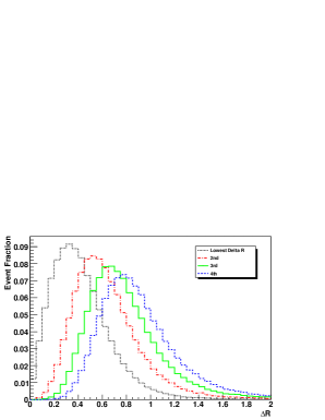
We expect that due to the large number of particles in the final state, the chance of reconstructible objects (such as jets) overlapping is large, so that the detector will frequently be unable to accurately reconstruct isolated objects. If two partons are very close in (roughly less than twice the diameter of the cone used in the jet algorithm), the jets coming from the partons are likely to be recombined into a single jet. Similarly, if a lepton is very close to a jet, it will likely not pass the isolation requirement. We utilize the standard cone jet reconstruction algorithm implemented in the PGS simulator, however we reduce the cone size to 0.4 in line with the expected performance of the ATLAS detector.
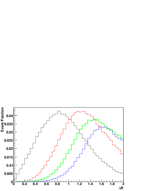
Figure 1 shows the distributions of the lowest, 2nd lowest, 3rd lowest, and 4th lowest values between reconstructible partons in four top events from benchmark model A. For comparison, the same information is also shown for Standard Model events. Here we define a reconstructible parton as any first/second generation quark or -quark. It may be seen in figure 1 (a) that in four top events there is a large likelihood of three to four pairs of overlapping objects, rendering reliable final state reconstruction difficult.
Direct reconstruction of top quarks in somewhat different decay chains has been studied in Ref. [26, 27]. We expect a similar study in our case will also yield at least some evidence that there are indeed top quarks in the event. Rather then presenting a detailed analysis here, we focus here on a somewhat different question. Clearly, in order to completely measure the branching ratios into different final states involving different numbers of top and bottom, it is not enough to just reconstruct a certain top quark. We need to be able to reconstruct all of the top quarks in the event with reasonable efficiency. However, our study already shows that there is a significant overlap between different object in this type of signal events. Including additional combinatorics, we expect a very low efficiency for reconstructing multiple tops.
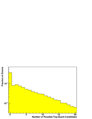
To gain some estimate of such efficiencies, we study how many tops we can possibly reconstruct in a event. To proceed, we define a ’top candidate’ to be the combination of two light-jets (ie non--tagged) and one -tagged jet, where the non--tagged dijet invariant mass satisfies GeV, the invariant mass of the b-jet with any lepton must satisfy GeV, while the invariant mass with either of the two non--tagged jets must satisfy GeV. Finally, the invariant mass of the final three-jet combination must satisfy GeV.
Figure 2 shows two distributions for the number of top candidates observed in our benchmark model A. The first figure, 2 (a), includes all possible three-quark combinations that satisfy the requirements above. The inherent combinatorical background due to the intense hadronic activity in four-top events is clearly visible. We see that the same -quark can be combined with other partons to form several “top candidates”. There can be no more than 4 top quarks present in the event, and the vast majority of ’candiate’ combinations are incorretly chosen. Figure 2 (b) shows the same information except that here we isolate only the distinct jet combinations of each event. Degeneracies that arise are removed by keeping track of the mass difference for each jet triplet, and choosing the set of triplets with the lowest average difference. From the figure, it is clear that this approach gives a significantly more reasonable result. However, notice that the number of reconstructed candidates drops dramatically as the top multiplicity increases, rendering statistical analysis essentially impossible without a large integrated luminosity.
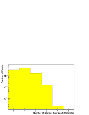
The study we perform here is not an actual reconstruction of the top quark. A true reconstruction involves positive identification of the top quark through statistical determination of the top invariant mass. Instead, this study is an estimate of how many objects obtained from recombining final states can be consistent with a top quark. We expect this study, though not completely precise, does capture the main effect of combinatorics and object merging. We observe that the efficiency for detecting one top quark as defined is approximately , for two quarks , three quarks , and for four quarks .
Further perfections of reconstruction techniques are certainly going to improve these results and should be pursued. However, it is likely that to extract statistically significant information based on a full reconstruction will still require large integrated luminosity.
5 Understanding multi-top final states
As we have demonstrated in the previous sections, new physics signals containing multiple tops can be discovered at the LHC. By direct reconstruction, we expect to gather evidence that there are indeed top quarks in the signal. However, there are many possible event topologies which can contribute to our signal. In general, gluino can decay into third generation quarks through , , and . Therefore, final states coming from gluino pair production can involve from zero to four top quarks, with relative amounts determined by gluino branching ratios. As we have argued in the introduction, measuring such branching ratios plays a central role in understanding the properties of superpartners involved. For example, the relative ratio of and could give us important information about the spectrum of the third generation squarks. At the same time, significant decay branching ratio of strongly suggests that either Higgsino or Wino (or both) is lighter than the gluino.
As demonstrated in the previous section, measuring the branching ratios by directly reconstructing top quarks suffers from low efficiencies. In this section, we will instead tackle this question from a different approach. We assume that the new physics signal has already been discovered in a set of channels, particularly those with multiple leptons and multiple bottom quarks (Table 4). In addition, there are a set of statistically significant experimental observables defined on the set of signal events. This general approach can in principle be applied in practice with an arbitrary set of experimental observables based on availability. Here, we will only use a limited set of experimental variables
-
•
2 -jets and either OS di-leptons, SS di-leptons, 3 leptons, 4 or more leptons
-
•
3 -jets and either 1 lepton, OS di-leptons, SS di-leptons, 3 leptons, 4 or more leptons
-
•
4 or more -jets and either 1 lepton, OS di-leptons, SS di-leptons, 3 leptons, 4 or more leptons
We will consider a general set of decay channels of the gluino which can in principle contribute to the new physics signal. We will consider as free parameters the relative branching ratios of those channels whose values are determined by a fit to the above set of experimental observables. This approach can be viewed as a natural application of the method proposed in Ref. [43]. The set of possible decay channels are chosen as follows
where we continue to used the short hand notation of not explicitly displaying either the lightest neutralino, or the lightest chargino. We have assumed that the lightest chargino and neutralino are nearly degenerate so that transitions between them will not yield observable decay products. indicates that we included the charge conjugated event.
The number of events in the possible decay channels are given by
These number can then be used to estimate the number of observed events with a particular signature, , which can receive contributions from several channels listed above with a particular fraction, , depending on event topology and experimental efficiencies. We have
In the rest of this section, we will first obtain estimates of all signal efficiencies . Then, we will perform a -fit to determine a set of best fit values of . Note that in order to obtain the branching ratio from these counting signatures, we will have to know the product . Such information could be available independently from other measurements, such as the gluino mass. We will show later in this section that our method indeed gives us an estimate of this absolute rate. At this moment, we note that we can already derive a lot of information about the underlying model if we measure the ratio of branching ratios, for which the dependence on drops out.
The key step in this method of fitting for branching ratios is, of course, to obtain an estimate the efficiencies, . Many factors enter in such an estimate. The existence of many objects, in particular jets, in the event means that simple extrapolation from single object efficiency is no longer reliable. In particular, there is a significant chance now for the leptons from top decay to be close to a jet and therefore fail the isolation cut. -tagging can also be affected. Numerical simulation using an appropriate model, a template, of the underlying physics involved is therefore unavoidable.
In practice, certain assumptions about the underlying model must be made in choosing a template. We have already chosen the set of channels to include, based on information gained from the type of study in the previous section. In addition, we have to choose the spectrum, the gluino mass and LSP mass, to be used in the template. To begin with, we will first choose a template model using the actual gluino mass and LSP mass as the underlying model. We will fit the underlying branching ratios by using efficiencies obtained by simulating this template and demonstrate such a fit does give us accurate information of the underlying model. We will then simulate a set of different templates with different mass hypotheses. We will show that for the variation of mass hypotheses we have studied, the difference induced for the fit does not significantly affect our conclusion about the underlying models. Of course, such a result still leaves the question of whether the range of variation of mass parameters we have used is too optimistic. Later in this section, we will show that indeed it is reasonable to expect we can get estimates of mass scales from other experimental observables so that we can choose our mass hypothesis with an error within this range. For the continuity of our presentation, we will present our result for the fits first. Then we will come back to address the question of choosing the mass hypothesis in detail.
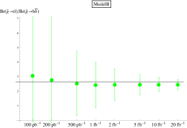
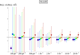

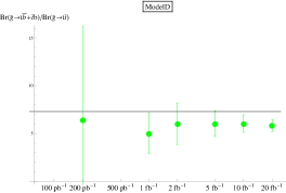
Our fit to BrBr for benchmark model-B using the correct mass hypothesis is shown in the left panel of Fig. 3. For this and all the other fits presented in this section, we have required that for a channel to be included in our fits, there must be at least 1 signal event, and the significance over the background must be greater than 3.
We pause here to briefly describe how error bars are calculated in these and the other fits presented in this section. Using large statistics for the template model, the statistical errors for calculating the efficiencies and for determining the number of events for a given signature are assumed to be much smaller that the expected Gaussian errors from the LHC data. The only errors we include here are statistical errors from the minimization procedure. Therefore, the error for a given branching ratio is given by the change in the branching ratio required to shift the one unit from its value at the minimum
From the left Fig. 3, we see that using the correct mass hypothesis, we will be able to measure the ratio BrBr with good accuracy for an integrated luminosity of fb-1. In particular, we will be able to verify that in Model B, the gluino decay is dominated by with a smaller but non-vanishing branching ratio for .
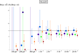
Next, we want to assess the effect of changing our assumptions of underlying spectrum. We will assume that although the mass spectrum cannot be precisely measured, some crude estimates can still be made based on kinematical variables such as and rate. We will provide justifications for this assumption later in this section. Therefore, we will consider cases where the gluino mass only deviates from the underlying benchmark model by about 100 GeV. In particular, we use four additional sets of alternative templates and carry out the same fit. The result in Model B is shown in the right panel of Fig. 3. We see that using different mass hypotheses does make a visible difference. However, we observe that these differences are not big enough to dramatically affect the information we will extract from our measurement of BrBr. In the case of 3-body gluino decay under consideration, this ratio is proportional to . Therefore, we see that using different mass hypotheses within this range will at most result in a factor two error in the measurement of the ratio of the branching ratios, will induce at most shift in the inferred ratio .
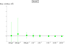
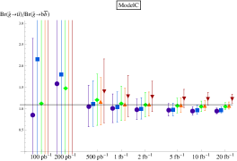
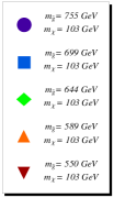
Notice that incorrect assumptions about the underlying spectrum do not lead to significant effects in the fitting when considering at least integrated luminosity of data. In all cases, we can still extract a good estimate of the squark hierarchy and the nature of the LSP.
Similar studies are performed for benchmark Model C. The result for Model C is shown in Fig. 4. Similar accuracies of the measurements are obtained with same integrated luminosity. In particular, we observe that we should be able to distinguish Model B and C from these results alone with about fb-1 of integrated luminosity.
As a final note, we add that the even for the correct mass template the ratio is slightly underestimated in all cases. This is because the data actually contains a small percentage of events in which the gluino decayed to first and second generation quarks. As those decays looks most similar the decay into two b-jets, the fit tends to slightly overestimate , and therefore underestimating .

The study of gluino decay for benchmark model D is presented in Fig. 5. In this case, we are interested in ratio BrBr. For a wino-LSP model like Model D, we expect this ratio to be large, which can indeed be experimentally verified with moderate luminosity, as shown in the figure.
We finally consider how well we can chose our mass hypotheses based on available experimental data. This is certainly an important issue since significantly wrong mass hypotheses lead to misleading results. To begin with, we study the dependence of our result on the mass hypothesis in more detail.
As the mass gap between the gluino and LSP is tightened, the events will have a harder time satisfying the missing energy cut we imposed. This more significantly affects events of the form than , since the tops will use more of the gluinos’ energy than the bottoms. Thus a tighter mass gap used in our template underestimates the ratio of efficiencies , see Figure 6. The fitter then adjusts for this low efficiency by fitting more events relative to the signature counts
Thus, in Models B and C as we increase(decrease) the gluino mass in our templates we tend to underestimate(overestimate) the branching ratio .
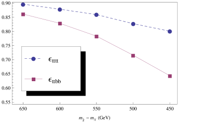
We see that the change in the mass gap between gluino and the LSP can account for most of the variation in the fit result. For example, extrapolating from our study, if our assumption of gluino mass is off by more than 200 GeV, the result for benchmark Model B will indeed look similar to that of Model C. However, since we expect to have significant excess in multiple channels, we observe that we should also have a significant amount of information about the mass scales, and in particular the mass gap of the new physics particles already at early stages of LHC running. For example, we would expect simple transverse variables in channels with multiple leptons (and hence lower Standard Model background) should already provide some indication of the mass scales involved.
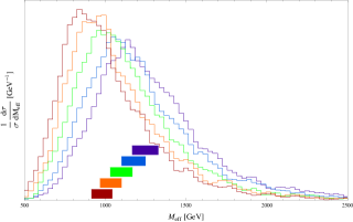

Indeed, visible differences can be seen between different gluino masses when we histogram the effective mass, , defined as the scalar sum of the transverse momentum for all objects in the an event
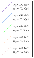
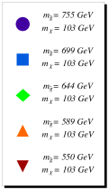
To demonstrate this, we plotted the effective mass for for the 5 gluino masses used in fits above, in Figure 7. The histogram curves move to lower energies (right to left) as the gluino mass is lowered. There is also a noticeable change in the effective mass spread, which we quantify as the location of middle quantile. The bars at the bottom show the location of the inner quantile; the highest one is for the largest gluino mass, the second highest for second largest gluino mass, etc. The fact that the bars move right to left as the gluino mass is lowered indicates that the median effective mass is decreasing, while the fact that the bars are shrinking indicate the effective mass has less variation as the gluino mass decreases.
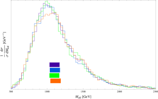
This analysis was only carried out for , so we still need to demonstrate that the effective mass is also independent of the gluino decay. To do this we plotted the effective mass for the four models considered in this paper, in Figure 8. The bars at the bottom show the spread, from top to bottom, for Model-A, Model-B, Model-C, and Model-D. As can be seen, the four histogram curves are remarkably similar, and have no noticeable differences in the median or spread.
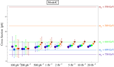
Notice that since our fit yield a set of values for with any given mass hypothesis. It can by itself provide a consistency check on the hypothesis. In particular, we can get a lower limit on the gluino pair production cross section, by summing and squaring the fit values
We can obtain cross sections for gluino pair production in the case of decoupled scalars, and rule out some incorrect gluino masses used in the templates. For example, in Model C (see Figure 9), we can rule out the GeV mass template at of data at certainty, and begin to rule out the GeV mass template at approximately of data at certainty. If the actual gluino is much lower than 600 GeV then there must be a significant branching fraction of the gluino that is not contributing the channels we used in our fits, such as gluino decays into first and second generation quarks.
6 Conclusion
We have studied the LHC signals of pair produced light gluinos which decay dominantly through , , and . We conclude that an early discovery of new physics in this scenario is possible due to significant excesses expected in multi-lepton multi-bottom channels. Measuring relative branching ratios of gluino decay into , and channels is essential to extract information about the underlying model. The crucial step in such a measurement is identify top multiplicity in the signal events. We show that direct reconstruction, while useful in gathering evidence for the existence top quark in decay products, is not sufficient to measure the number of top quarks in the event effectively. We proposed and studied a method based on fitting a set of branching ratios to a collection of experimental observables, most of them inclusive counts. Efficiencies for identifying a particular final state resulting from certain underlying decay topology are estimated by simulating corresponding templates. We conclude that this method will allow us to learn about gluino decay branching ratios with roughly 10 of integrated luminosity. We verified that, in combination with earlier information on the mass spectrum of gluino and the LSP, we can obtain a reliable measurement by choosing appropriate mass hypotheses. We emphasize that the main advantage of our method is that it allows us to use a large number of channels, many of them with multiple leptons and bottoms, in which we expect to see excesses during the early stage of LHC in models of this sort.
We showed that we can expect to gain enough information about the mass spectrum, in particular the mass gap , from simple observables like effective mass and demonstrated that, with our fitting method, it is also possible to obtain an estimate of the gluino production cross section which in turn gives us very valuable information of the gluino mass, which also gives a consistency check of the assumption we made in our measurement of the branching ratio.
In the paper, we have considered only benchmark models with only a set of simple decay chains. More complicated models will certainly contain channels which requires further study [26, 27]. For example, a decay chain which contains followed by has the same set of final state particles as top decay. On the other hand, we have also only used counting signatures in our fit. Inclusion of more kinematical variables may improve our ability of discerning other decay topologies. For example, in the decay of stop mentioned above, the kinematics of and will be in general different from the case of top decay.
One key factor entering our lepton efficiency is the isolation requirement. This is particularly significant in our case since we expect to have a lot of hadronic activity in these top rich events. We have only implemented a simple and commonly used isolation criterion based on hadronic activity within a narrow cone around the lepton. However, one can in principle improve and optimize the isolation cuts by including additional alternative isolation criteria, such as by requiring the invariant mass of lepton and the hadronic activity . This cut is effective since a lepton from heavy flavor decay is typically soft and therefore gives a small , while it is expected to be larger for accidental overlap between lepton and jet.
7 Acknowledgement
We are grateful for interesting discussions with Aaron Pierce and David Morrissey. L.-T. W. is supported by the National Science Foundation under grant PHY-0756966 and the Department of Energy under grant DE-FG02-90ER40542. G.L.K., E.K. and P.G. are supported in part by the U.S. D.O.E. B.S.A and L.-T.W. thank the Michigan Center for Theoretical Physics for hospitality during which this work was done. G.L.K. thanks IAS for hospitality. E.K. thanks Princeton University for hospitality. P.G. thanks the Abdus Salam International Center for Theoretical Physics for hospitality.
References
- [1] T. Gherghetta and A. Pomarol, Nucl. Phys. B 586, 141 (2000) [arXiv:hep-ph/0003129]. K. Agashe, A. Delgado, M. J. May and R. Sundrum, JHEP 0308, 050 (2003) [arXiv:hep-ph/0308036].
- [2] S. Dimopoulos and H. Georgi, Nucl. Phys. B 193, 150 (1981).
- [3] T. Appelquist, H. C. Cheng and B. A. Dobrescu, Phys. Rev. D 64, 035002 (2001) [arXiv:hep-ph/0012100].
- [4] N. Arkani-Hamed, A. G. Cohen and H. Georgi, Phys. Lett. B 513, 232 (2001) [arXiv:hep-ph/0105239].
- [5] Z. Chacko, H. S. Goh and R. Harnik, Phys. Rev. Lett. 96, 231802 (2006) [arXiv:hep-ph/0506256].
- [6] K. Agashe, A. Belyaev, T. Krupovnickas, G. Perez and J. Virzi, Phys. Rev. D 77, 015003 (2008) [arXiv:hep-ph/0612015]. V. Barger, T. Han and D. G. E. Walker, Phys. Rev. Lett. 100, 031801 (2008) [arXiv:hep-ph/0612016]. B. Lillie, L. Randall and L. T. Wang, JHEP 0709, 074 (2007) [arXiv:hep-ph/0701166]. A. L. Fitzpatrick, J. Kaplan, L. Randall and L. T. Wang, JHEP 0709, 013 (2007) [arXiv:hep-ph/0701150]. K. Agashe, H. Davoudiasl, G. Perez and A. Soni, Phys. Rev. D 76, 036006 (2007) [arXiv:hep-ph/0701186]. U. Baur and L. H. Orr, Phys. Rev. D 76, 094012 (2007) [arXiv:0707.2066 [hep-ph]]. R. Frederix and F. Maltoni, arXiv:0712.2355 [hep-ph]. U. Baur and L. H. Orr, arXiv:0803.1160 [hep-ph]. J. Thaler and L. T. Wang, JHEP 0807, 092 (2008) [arXiv:0806.0023 [hep-ph]]. D. E. Kaplan, K. Rehermann, M. D. Schwartz and B. Tweedie, Phys. Rev. Lett. 101, 142001 (2008) [arXiv:0806.0848 [hep-ph]]. L. G. Almeida, S. J. Lee, G. Perez, G. Sterman, I. Sung and J. Virzi, arXiv:0807.0234 [hep-ph]. L. G. Almeida, S. J. Lee, G. Perez, I. Sung and J. Virzi, arXiv:0810.0934 [hep-ph].
- [7] G. Brooijmans, ATLAS note, ATL-PHYS-CONF-2008-008.
- [8] Y. Bai and Z. Han, arXiv:0809.4487 [hep-ph].
- [9] H. C. Cheng, I. Low and L. T. Wang, Phys. Rev. D 74, 055001 (2006) [arXiv:hep-ph/0510225]. P. Meade and M. Reece, Phys. Rev. D 74, 015010 (2006) [arXiv:hep-ph/0601124]. A. Freitas and D. Wyler, JHEP 0611, 061 (2006) [arXiv:hep-ph/0609103]. A. Belyaev, C. R. Chen, K. Tobe and C. P. Yuan, arXiv:hep-ph/0609179. S. Matsumoto, M. M. Nojiri and D. Nomura, Phys. Rev. D 75, 055006 (2007) [arXiv:hep-ph/0612249]; M. M. Nojiri and M. Takeuchi, arXiv:0802.4142 [hep-ph]. T. Han, R. Mahbubani, D. G. E. Walker and L. T. Wang, arXiv:0803.3820 [hep-ph].
- [10] R. Contino and G. Servant, JHEP 0806, 026 (2008) [arXiv:0801.1679 [hep-ph]].
- [11] S. Kraml and A. R. Raklev,
- [12] B. Lillie, J. Shu and T. M. P. Tait, JHEP 0804, 087 (2008) [arXiv:0712.3057 [hep-ph]].
- [13] For a recent review on top quark related new physics signatures, see T. Han, arXiv:0804.3178 [hep-ph].
- [14] For a recent review, see D. J. H. Chung, L. L. Everett, G. L. Kane, S. F. King, J. D. Lykken and L. T. Wang, Phys. Rept. 407, 1 (2005) [arXiv:hep-ph/0312378].
- [15] M. Gerbush, T. J. Khoo, D. J. Phalen, A. Pierce and D. Tucker-Smith, Phys. Rev. D 77, 095003 (2008) [arXiv:0710.3133 [hep-ph]].
- [16] A. R. Zerwekh, C. O. Dib and R. Rosenfeld, Phys. Rev. D 77, 097703 (2008) [arXiv:0802.4303 [hep-ph]]. P. Fileviez Perez, R. Gavin, T. McElmurry and F. Petriello, arXiv:0809.2106 [hep-ph]. T. Plehn and T. M. P. Tait, arXiv:0810.3919 [hep-ph].
- [17] B. A. Dobrescu, K. Kong and R. Mahbubani, arXiv:0709.2378 [hep-ph].
- [18] P. Langacker, G. Paz, L. T. Wang and I. Yavin, Phys. Rev. Lett. 100, 041802 (2008) [arXiv:0710.1632 [hep-ph]]. H. Verlinde, L. T. Wang, M. Wijnholt and I. Yavin, JHEP 0802, 082 (2008) [arXiv:0711.3214 [hep-th]]. P. Langacker, G. Paz, L. T. Wang and I. Yavin, Phys. Rev. D 77, 085033 (2008) [arXiv:0801.3693 [hep-ph]].
- [19] L. L. Everett, I. W. Kim, P. Ouyang and K. M. Zurek, JHEP 0808, 102 (2008) [arXiv:0806.2330 [hep-ph]]. L. L. Everett, I. W. Kim, P. Ouyang and K. M. Zurek, Phys. Rev. Lett. 101, 101803 (2008) [arXiv:0804.0592 [hep-ph]]. S. Nakamura, K. i. Okumura and M. Yamaguchi, Phys. Rev. D 77, 115027 (2008) [arXiv:0803.3725 [hep-ph]]. K. Choi, K. S. Jeong, S. Nakamura, K. I. Okumura and M. Yamaguchi, arXiv:0901.0052 [hep-ph].
- [20] B. S. Acharya, K. Bobkov, G. L. Kane, J. Shao and P. Kumar, arXiv:0801.0478 [hep-ph].
- [21] J. J. Heckman and C. Vafa, arXiv:0809.3452 [hep-ph].
- [22] A. G. Cohen, D. B. Kaplan, F. Lepeintre and A. E. Nelson, Phys. Rev. Lett. 78 (1997) 2300 [arXiv:hep-ph/9610252].
- [23] J. L. Feng, K. T. Matchev and T. Moroi, Phys. Rev. D 61 (2000) 075005 [arXiv:hep-ph/9909334].
- [24] N. Arkani-Hamed and S. Dimopoulos, JHEP 0506 (2005) 073 [arXiv:hep-th/0405159]. G. F. Giudice and A. Romanino, Nucl. Phys. B 699 (2004) 65 [Erratum-ibid. B 706 (2005) 65] [arXiv:hep-ph/0406088]. N. Arkani-Hamed, S. Dimopoulos, G. F. Giudice and A. Romanino, Nucl. Phys. B 709 (2005) 3 [arXiv:hep-ph/0409232].
- [25] H. Baer, X. Tata and J. Woodside, “PHENOMENOLOGY OF GLUINO DECAYS VIA LOOPS AND TOP QUARK YUKAWA COUPLING,” Phys. Rev. D 42, 1568 (1990).
- [26] J. Hisano, K. Kawagoe, R. Kitano and M. M. Nojiri, “Scenery from the top: Study of the third generation squarks at CERN LHC,” Phys. Rev. D 66, 115004 (2002) [arXiv:hep-ph/0204078].
- [27] J. Hisano, K. Kawagoe and M. M. Nojiri, “A detailed study of the gluino decay into the third generation squarks at
- [28] P. G. Mercadante, J. K. Mizukoshi and X. Tata, Braz. J. Phys. 37, 549 (2007).
- [29] H. Baer, V. Barger, G. Shaughnessy, H. Summy and L. t. Wang, Phys. Rev. D 75, 095010 (2007) [arXiv:hep-ph/0703289].
- [30] P. Gambino, G. F. Giudice and P. Slavich, “Gluino decays in split supersymmetry,” Nucl. Phys. B 726, 35 (2005) [arXiv:hep-ph/0506214].
- [31] M. Toharia and J. D. Wells, “Gluino decays with heavier scalar superpartners,” JHEP 0602, 015 (2006) [arXiv:hep-ph/0503175].
- [32] R. Bonciani, S. Catani, M. L. Mangano and P. Nason, “NLL resummation of the heavy-quark hadroproduction cross-section,” Nucl. Phys. B 529, 424 (1998) [arXiv:hep-ph/9801375].
- [33] T. Sjostrand, S. Mrenna and P. Skands, “PYTHIA 6.4 physics and manual,” JHEP 0605, 026 (2006) [arXiv:hep-ph/0603175].
- [34] J. Alwall et al., “MadGraph/MadEvent v4: The New Web Generation,” JHEP 0709, 028 (2007) [arXiv:0706.2334 [hep-ph]].
- [35] S. Catani, F. Krauss, R. Kuhn and B. R. Webber, JHEP 0111, 063 (2001) [arXiv:hep-ph/0109231].
- [36] John Conway, “http://www.physics.ucdavis.edu/ conway/research/software/pgs/pgs4-general.htm’
- [37] W. Beenakker, R. Hopker, M. Spira and P. M. Zerwas, Nucl. Phys. B 492, 51 (1997) [arXiv:hep-ph/9610490].
- [38] See, for example, H. Baer, C. h. Chen, F. Paige and X. Tata, Phys. Rev. D 53 (1996) 6241 [arXiv:hep-ph/9512383].
- [39] H. Baer, H. Prosper and H. Summy, Phys. Rev. D 77, 055017 (2008) [arXiv:0801.3799 [hep-ph]].
- [40] Z. Sullivan and E. L. Berger, Phys. Rev. D 78, 034030 (2008) [arXiv:0805.3720 [hep-ph]].
- [41] B. S. Acharya, F. Cavallari, G. Corcella, R. Di Sipio and G. Petrucciani, “Re-discovery of the top quark at the LHC and first measurements,” arXiv:0806.0484 [hep-ex].
- [42] M. M. Nojiri, G. Polesello and D. R. Tovey, arXiv:hep-ph/0312318.
- [43] N. Arkani-Hamed, P. Schuster, N. Toro, J. Thaler, L. T. Wang, B. Knuteson and S. Mrenna, arXiv:hep-ph/0703088.