Spatial correlation properties of the anomalous density matrix
in a slab of nuclear matter with realistic NN-forces

Abstract

Spatial correlation characteristics of the anomalous density matrix $\varkappa$ in a slab of nuclear matter with the Paris and Argonne v₁₈ forces are calculated. A detailed comparison with predictions of the effective Gogny force is made. It is found that the two realistic forces lead to very close results which are qualitatively similar to those for the Gogny force. At the same time, the magnitude of $\varkappa$ for realistic forces is essentially smaller than the one for the Gogny force. The correlation characteristics are practically independent of the magnitude of $\varkappa$ and turn out to be quite close for the three kinds of the force. In particular, all of them predict a small value of the local correlation length at the surface of the slab and a big one, inside. These results are in agreement with those obtained recently by Pillet at al. for finite nuclei with the Gogny force.

I Introduction

The problem of surface nature of nuclear pairing has a long history, see the review paper Rep and Refs. therein. First, it was formulated in terms of the effective pairing interaction (EPI) entering the gap equation in a model space in which the pairing problem is usually considered. Within the self-consistent Finite Fermi System theory, the use of a natural density dependent ansatz for the EPI has resulted in a strong attraction at the nuclear surface, being rather small inside nuclei ZvSap . Similar conclusion was obtained in the ab initio calculation of the EPI BLSZ1 . Later, the surface enhancement of the gap function $\Delta(X)$ was found by solving the gap equation for the complete Hilbert space in semi-infinite nuclear matter with the realistic Paris force in BLSZ2 and with the effective Gogny force in FarSch . Similar conclusions were obtained for a nuclear slab in Ref. 6auth where the gap equation was solved for both the types of NN force simultaneously. It was found that, although there is a quntitative difference between predictions of the two calculations, both of them show a pronounced maximum of $\Delta(X)$ at the surface of the slab, $X=L$, where $2L$ is the slab width, the effect being stronger for smaller values of $L$. In more detail, the gap equation for the nuclear slab was solved in Pankr1 for the Paris force and in Pankr2 for the Argonne v₁₈ force. It turned out that predictions of these two absolutely different kinds of realistic NN-force for the gap function agree with each other within 10%, both yielding the ratio $\Delta(X\simeq L)/\Delta(X=0)\simeq 2$.

Recently, Pillet et al. PiSanSch investigated directly spatial properties of the anomalous density $\varkappa$ which determines the space distribution of Cooper pairs. Calculations were carried out within the HFB approach with employing the D1S Gogny interaction Gogny for a set of Sn, Ni, and Ca isotopes. It was shown that Cooper pairs in nuclei preferentially are located with small size ($2-3\;$fm) in the surface region. The relevance of this phenomenon to two-nucleon transfer reactions was discussed. It should be mentioned that earlier the correlation properties of pairing for specific nuclei were studied by Catara et. al. Catara , Ferreira et al. Ferreira , Bertsch et al. Bertsch , Hagino et al. a12 and yet in several works cited in PiSanSch . A similar investigation has also been performed for $T=0$ pairing in dilute nuclear matter L_Sch .

In this paper we carry out an analogous study for a nuclear slab with realistic NN force (the Paris and Argonne v₁₈ potentials) and the Gogny force. Our goal is to compare predictions for the correlation pairing characteristics of the Gogny force and of realistic forces in order to analyze, to what extent the effect found in PiSanSch is general and independent on the specific choice of NN force. It should be mentioned that, with small modifications, the nuclear slab configuration may be used to describe the so-called “lasagna” phase of the inner crust of neutron stars.

II Main definitions

To make the comparison easier, let us recall the main definitions introduced in PiSanSch . In a inhomogeneous system, the anomalous density matrix is defined as follows:

$$\varkappa({\bf r}_{1},{\bf r}_{2})=\sum_{i}u_{i}({\bf r}_{1})v_{i}({\bf r}_{2}),$$ (1)

where $u_{i}({\bf r}),v_{i}({\bf r})$ are the Bogolyubov functions. For a spherical nucleus, it is convenient to go to relative and center of mass coordinates, ${\bf r}={\bf r}_{1}-{\bf r}_{2}$ and ${\bf R}=({\bf r}_{1}+{\bf r}_{2})/2$. In PiSanSch the anomalous density matrix was studied in such a way that the probability distribution of Cooper pairs, $|\varkappa({\bf R},{\bf r})|^{2}$, was averaged over the angle between the vectors ${\bf R}$ and ${\bf r}$,

$$\varkappa^{2}(R,r)=\frac{1}{4\pi}\int|\varkappa({\bf R},{\bf r})|^{2}\;d\Omega\;.$$ (2)

In particular, the space distribution of the pairing tensor $|\varkappa(R,r)|^{2}$ was analyzed. The probability distribution of pairing correlations,

$$P(R,r)=R^{2}r^{2}\varkappa^{2}(R,r)\,,$$ (3)

was calculated in PiSanSch . To avoid misunderstanding, this quantity is not normalized to unity.

The coordinate dependent local correlation length was defined as

$$\xi(R)=\frac{(\int r^{2}\varkappa^{2}(R;r)\;d^{3}r)^{1/2}}{(\int\varkappa^{2}(R;r)\;d^{3}r)^{1/2}}\;.$$ (4)

At last, the locally normalized pairing tensor was considered in the form

$$W(R,r)=\dfrac{r^{2}\varkappa^{2}(R,r)}{\int\varkappa^{2}(R,r)\;r^{2}dr}\;,$$ (5)

as it enters the definition of the correlation length.

Just as in Pankr2 , we consider a nuclear slab embedded into the Saxon-Woods potential $U(x)$ symmetrical with respect to the point $x=0$ with potential well depth $U_{0}=-50\;$MeV and diffuseness parameter of $d=0.65\;$fm typical for finite nuclei. The chemical potential is taken equal to $\mu=-8\;$MeV. To compare our calculations with those of PiSanSch , we fixed the thickness parameter of the slab as $L=6\;$fm to mimic nuclei of the tin region. We use the notation ${\bf r}=({\bf s},x)$, where ${\bf s}$ is the two-dimensional vector in the plane perpendicular to the $x$-axis. The system under consideration is homogeneous in the ${\bf s}$-plane, therefore one has $\varkappa({\bf r}_{1},{\bf r}_{2})\to\varkappa({\bf R},{\bf r})\to\varkappa(X;x,{\bf s})$, with the obvious notation. The definition (4) is then rewritten as follows:

$$\xi^{2}(X)=\dfrac{\int(x^{2}+s^{2})|\varkappa(X;x,{\bf s})|^{2}\;d^{3}r}{\int|\varkappa(X;x,{\bf s})|^{2}\;d^{3}r}\;.$$ (6)

As far as the correlation properties in the $x$-direction and in the ${\bf s}$-plane are essentially different, it looks reasonable to consider them separately,

$$\xi^{2}(X)=\xi_{x}^{2}(X)+\xi_{s}^{2}(X)\;,$$ (7)

with the obvious notation.

In the slab geometry, the angular averaging procedure similar to that in Eq. (2) is as follows:

$$\varkappa^{2}(X,r)=\frac{1}{4\pi}\int|\varkappa(X;x,{\bf s})|^{2}\;\dfrac{2}{r}\;\delta(r^{2}-x^{2}-s^{2})\;d^{2}s\;dx\;.$$ (8)

It gives the distribution of the pairing tensor for a fixed value of the 3-dimensional relative distance $r$. There is another possibility, just to integrate over ${\bf s}$:

$$\varkappa^{2}(X,x)=\int|\varkappa(X;x,{\bf s})|^{2}\;d^{2}s\;.$$ (9)

It yields the quantity $\varkappa^{2}(X,x)$ which gives the distribution of the pairing tensor in natural for slab variables. For brevity, we use the same notation for the integrated anomalous density matrix as for the initial one and the one in Eq. (8). The arguments should help to avoid misleading. Note that $\varkappa(X,x)$ and $\varkappa(X,r)$ have different dimensions.

Figure 1: The gap $\Delta(k=k_{\mbox{\scriptsize F}})$ in infinite nuclear matter

Figure 2: The correlation pairing length in infinite nuclear matter

III Calculation results

Methods of solving the gap equation and the Bogolyubov equations for a nuclear slab are described in Pankr1 for the separable representation of the Paris potential and in Pankr2 , for the Argonne v₁₈ force. The latter could be used for arbitrary NN-potential, and we repeated all the calculations of Pankr2 for the Gogny force. To begin the comparison, let us start from infinite nuclear matter. The dependence of the gap on the density of nuclear matter for the three kinds of the NN-force is displayed in Fig. 1. The correlation length (4) in infinite matter can be easily found in the momentum space:

$$\xi^{2}=\dfrac{\int\left|\dfrac{\partial}{\partial k}\varkappa(k)\right|^{2}d^{3}k}{\int|\varkappa(k)|^{2}d^{3}k}.$$ (10)

Let us substitute in this equation $\varkappa(k)=\Delta(k)/2E_{k}$, where $E_{k}=\sqrt{(\varepsilon_{k}-\varepsilon_{\mbox{\scriptsize F}})^{2}+\Delta^{2}(k)}$, $\varepsilon_{k}=k^{2}/2m^{*}$, $\varepsilon_{\mbox{\scriptsize F}}=k_{\mbox{\scriptsize F}}^{2}/2m^{*}$. The functions inside the integrals both in the numerator and denominator of this relation are very peaked in the vicinity of $k=k_{\mbox{\scriptsize F}}$ and rapidly vanish outside the interval $|k-k_{\mbox{\scriptsize F}}|\stackrel{{\scriptstyle\scriptstyle<}}{{\phantom{}{}_{\sim}}}k_{\mbox{\scriptsize F}}(\Delta_{\mbox{\scriptsize F}}/\varepsilon_{\mbox{\scriptsize F}})$, $\Delta_{\mbox{\scriptsize F}}=\Delta(k_{\mbox{\scriptsize F}})$. Usually one deals with the limit $(\Delta_{\mbox{\scriptsize F}}/\varepsilon_{\mbox{\scriptsize F}})<<1$. In this case, one can substitute $\Delta(k)=\Delta_{\mbox{\scriptsize F}}$ in Eq. (10) and evaluate the integrals analytically. A simple calculation yields

$$\xi=\frac{v_{\mbox{\scriptsize F}}}{\sqrt{8}\Delta_{\mbox{\scriptsize F}}}\;,$$ (11)

where $v_{\mbox{\scriptsize F}}=k_{\mbox{\scriptsize F}}/m^{*}$.

The correlation length for the three kinds of force under discussion found numerically from Eq. (10), with $m^{*}=m$, are displayed in Fig. 2. For comparison, the approximate $\xi$ from Eq. (11) with Argonne force is also displayed. It is seen that the approximate formula works sufficiently well in all the interval of $k_{\mbox{\scriptsize F}}$. Even at the maximum of the gap the deviation from the numerical result is of the order of 15%.

One can see that at small density, $k_{\mbox{\scriptsize F}}<0.5\;$fm^-1, the results for all three forces practically coincide. This is not strange. Indeed, although the Gogny force is an effective one, in the ${}^{1}S_{0}$ channel under consideration it describes the free NN-scattering perfectly well for small energy values which are only important in this density interval. In this sense, the Gogny force could be considered as a semi-realistic force. Two realistic forces lead to close results for all density values. In the vicinity of the gap maximum, the difference between $\Delta^{\rm Arg}$ and $\Delta^{\rm Par}$ does not exceed 10%, and only at $k_{\mbox{\scriptsize F}}\simeq 1.4\;$fm^-1, where the gap value itself becomes very small, the relative difference becomes larger. As to the Gogny force, at the density region $k_{\mbox{\scriptsize F}}\simeq 1\;$fm^-1 it leads to the gap values which are bigger by approximately $(20\div 30)$% than those for realistic forces. Correspondingly, the correlation length for the Gogny force is quite close to that of the realistic forces till $k_{\mbox{\scriptsize F}}\simeq 0.8\;$fm^-1, and only at $k_{\mbox{\scriptsize F}}\simeq 1.2\;$fm^-1 the difference becomes large. The density dependence of the correlation length, $\xi(k_{\mbox{\scriptsize F}})$, is qualitatively similar for all the three types of force. It consists of a plateau at $0.3\stackrel{{\scriptstyle\scriptstyle<}}{{\phantom{}{}_{\sim}}}k_{\mbox{\scriptsize F}}\stackrel{{\scriptstyle\scriptstyle<}}{{\phantom{}{}_{\sim}}}1\;$fm^-1 and two intervals of sharp growth, at $k_{\mbox{\scriptsize F}}\stackrel{{\scriptstyle\scriptstyle<}}{{\phantom{}{}_{\sim}}}0.3\;$fm^-1 and $k_{\mbox{\scriptsize F}}\stackrel{{\scriptstyle\scriptstyle>}}{{\phantom{}{}_{\sim}}}1\;$fm^-1. In the latter, the value of $\xi^{\rm Gog}(k_{\mbox{\scriptsize F}})$ is growing with $k_{\mbox{\scriptsize F}}$ much slower than that of $\xi^{\rm Arg}(k_{\mbox{\scriptsize F}})$ and $\xi^{\rm Par}(k_{\mbox{\scriptsize F}})$. Note that at $k_{\mbox{\scriptsize F}}\stackrel{{\scriptstyle\scriptstyle>}}{{\phantom{}{}_{\sim}}}1.2\;$fm^-1 the difference between $\xi^{\rm Arg}(k_{\mbox{\scriptsize F}})$ and $\xi^{\rm Par}(k_{\mbox{\scriptsize F}})$ also becomes noticeable. This is a manifestation of their behavior near the critical point $k_{\mbox{\scriptsize F}}^{\rm c}$ at which the gap vanishes and transition to the normal phase of nuclear matter occurs. The values of $k_{\mbox{\scriptsize F}}^{\rm c}$ for the Argonne force and the Paris potential are a little different. This results in different behavior of $\xi^{\rm Arg}(k_{\mbox{\scriptsize F}})$ and $\xi^{\rm Par}(k_{\mbox{\scriptsize F}})$ in the region of $k_{\mbox{\scriptsize F}}\simeq 1.5\;$fm^-1.

Figure 3: The Fermi averaged gap $\Delta_{\mbox{\scriptsize F}}(X)$

Figure 4: The Fermi averaged effective pairing interaction ${\mathcal{V}}^{\mbox{\scriptsize F}}_{\mbox{\scriptsize eff}}(X)$

Figure 5: The correlation pairing length $\xi(X)$ in a slab of nuclear matter

Figure 6: The correlation pairing length $\xi_{x}(X)$ in the $x$-direction for a slab of nuclear matter

Let us now turn to the slab system. Before analyzing the correlation characteristics, it is instructive to briefly compare the EPI and the gap itself found with the realistic forces and the Gogny force. The “Fermi averaged” gap is displayed in Fig.3. It is defined as follows:

$$\Delta_{\mbox{\scriptsize F}}(X)=\Delta(X,k_{\mbox{\scriptsize F}}(X))\,,$$ (12)

where the local Fermi momentum is $k_{\mbox{\scriptsize F}}(X){=}\sqrt{2m(\mu{-}U(X))}\;\Theta(\mu{-}U(X))$. This quantity characterizes the gap on average Rep ; Pankr1 ; Pankr2 . We see, first, that all three functions $\Delta_{\mbox{\scriptsize F}}(X)$ have pronounced maxima at $X\simeq L=6\;fm$. The ratio $\Delta_{\mbox{\scriptsize F}}(X\simeq L)/\Delta_{\mbox{\scriptsize F}}(X=0)\simeq 2$ for realistic forces and $\simeq 1.5$ for the Gogny force, in agreement with 6auth . Second, the gap $\Delta_{\mbox{\scriptsize F}}^{\rm Gog}$ is significantly bigger than $\Delta_{\mbox{\scriptsize F}}^{\rm Par}$ and $\Delta_{\mbox{\scriptsize F}}^{\rm Arg}$, by approximately a factor one and a half at the surface and two inside the slab. It is worth to discuss this point in more detail. Let us consider ¹²⁰Sn as a “reference nucleus”. Its empirical gap value is estimated usually as $\Delta\simeq 1.3\;$MeV Fay ; milan . Diagonal matrix elements of the gap found in Pankr1 ; Pankr2 for a slab with $L=6\;$fm are about 1 MeV which agrees with the above value, leaving a room about 20–30% for the surface vibration contribution. The latter was estimated in milan as $\simeq 50$% which is, in our opinion, too much, see discussion in Rep . We consider the estimation of A_Kam at $\simeq 30$% as more realistic, but, evidently, also too big, because of disregarding so-called tadpole diagrams Kam_S . Calculations of PiSanSch for this nucleus gave $\Delta\simeq 2\;$MeV which, in our opinion, is too much, especially if to take into account that some additional contribution of surface vibrations to the mean field theory value of $\Delta$ should be! Thus, our observation in slab calculations that the Gogny force overestimates the gap value agrees essentially with results of PiSanSch .

To understand the physical reason for the surface enhancement of the pairing gap with each NN force under consideration and bigger values of the gap for Gogny force, it is useful to calculate the EPI which we use in the two-step method of solving the gap equation Rep . Let us remind how this quantity is defined. In a symbolic form, the microscopic gap equation reads:

$$\Delta={\cal V}A^{s}\Delta\,,$$ (13)

where ${\cal V}$ is the free $NN$-potential and $A^{s}=GG^{s}$ stands for the two-particle propagator in the superfluid system. Here $G$ and $G^{s}$ are the one-particle Green functions without and with pairing effects taken into account, respectively. In Eq. (13), as usual, integration over intermediate coordinates and summation over spin variables is understood. Let us now split the complete Hilbert space $S$ of two-particle states into two parts, $S=S_{0}+S^{\prime}$. The first one is the model subspace $S_{0}$ in which the gap equation is considered, and the other is the complementary subspace $S^{\prime}$. They are separated by the energy $E_{0}$ in such a way that $S_{0}$ involves all the two-particle states $(\lambda,\lambda^{\prime})$ with the single-particle energies $\varepsilon_{\lambda},\varepsilon_{\lambda^{\prime}}<E_{0}$. The complementary subspace $S^{\prime}$ involves the two-particle states for which one of the energies $\varepsilon_{\lambda},\varepsilon_{\lambda^{\prime}}$ or both of them are greater than $E_{0}$. Therefore, pairing effects can be neglected in $S^{\prime}$ if $E_{0}$ is sufficiently large. The validity of inequality $\Delta^{2}/(E_{0}-\mu)^{2}\ll 1$ is the criterium of such approximation. Correspondingly, the two-particle propagator is represented as the sum $A^{s}=A^{s}_{0}+A^{\prime}$. Here we already neglected the superfluid effects in the $S^{\prime}$-subspace and omitted the superscript “s” in the second term. The gap equation (13) can be rewritten in the model subspace,

$$\Delta=V^{p}_{\mbox{\scriptsize eff}}\,A^{s}_{0}\,\Delta\,,$$ (14)

where the EPI should be found in the supplementary subspace,

$$V^{p}_{\mbox{\scriptsize eff}}={\cal V}+{\cal V}A^{\prime}\,V^{p}_{\mbox{\scriptsize eff}}\,.$$ (15)

Note that the last equation has a strong similarity with the Bethe–Goldstone equation.

As the analysis showed Pankr1 ; Pankr2 , the optimal choice of splitting corresponds to $E_{0}=15\div 20\;$MeV. In a slab system, the EPI is calculated in the mixed coordinate-momentum representation Rep . To illustrate graphically properties of the EPI, we present it in a localized form Pankr1 ; Pankr2 with the Fermi averaged strength

$${\mathcal{V}}^{\mbox{\scriptsize F}}_{\mbox{\scriptsize eff}}(X)=\int dtV^{p}_{\mbox{\scriptsize eff}}(k_{1}{=}k_{2}{=}k_{\mbox{\scriptsize F}}(X);X+\frac{t}{2},X-\frac{t}{2})\,.$$ (16)

The Fermi averaged EPI for the Argonne v₁₈ force and the Gogny D1S force calculated for $E_{0}=15\;$MeV are displayed in Fig.4. We did not display the EPI for the Paris potential as it practically coincides with that for the Argonne force. One can see that both the curves behave in a similar way changing from quite week attraction inside the slab to very strong one outside. The reason for the latter is that in the asymptotic region $X>L$ the ${\mathcal{V}}^{\mbox{\scriptsize F}}_{\mbox{\scriptsize eff}}$ value tends to the quantity which is very close to the free $T$-matrix taken at the negative energy $E=2\mu$. To be precise, the limit is equal to $T(E=2\mu)$ if the separating energy $E_{0}=0$. In the case of $E_{0}\neq 0$ the limit is equal to some “$T^{\prime}$-matrix” which is obtained by solving the same Lippman–Schwinger equation as the $T$-matrix, but in a cut momentum space, because the contribution of nucleons with total energy less than $E_{0}$ must be pulled out. As it is known, the Gogny force leads to the scattering length in the ${}^{1}S_{0}$ channel $a\simeq 12\;$fm Bertsch ; a12 . It differs, of course, from the experimental value of $a\simeq 18\;$fm which is reproduced by any realistic force, but not so much. In any case, the virtual pole of the $T$-matrix for the Gogny force is close to zero as it should be. Therefore the analytical continuation of the $T$-matrix (or $T^{\prime}$-matrix) to rather small negative energy $E=2\mu$ results in an enhancement of the $T^{\prime}$-matrix ($\simeq-950\;$MeV fm³) in comparison with typical values. This enhancement is not so strong as in the case of the Argonne force ($\simeq-1100\;$MeV fm³), but it is equally significant. The inner value of the EPI for the Gogny force is quite small ($\simeq-160\;$MeV fm³), but bigger than for the Argonne one ($\simeq-95\;$MeV fm³). In our previous study with realistic forces Rep ; Pankr1 ; Pankr2 we explained the surface enhancement of the gap in terms of the sharp variation of the EPI at the surface. In the case of the Argonne force, the ratio ${\cal V}^{\rm out}_{\mbox{\scriptsize eff}}/{\cal V}^{\rm in}_{\mbox{\scriptsize eff}}\simeq 12$. For the Gogny force, it is about 6. This is also a big number leading to a surface enhancement of the gap, but not so pronounced as for realistic force. Fig.4 explains also why the Gogny gap is so big. It is well known that the pairing gap depends on the interaction strength in an exponential way. In Pankr1 it was found that 1% variation of ${\cal V}^{\rm in}_{\mbox{\scriptsize eff}}$ leads to 5% variation of the gap. It explains why the gap function for the Gogny force is in $1.5\div 2$ times greater than the one for realistic forces.

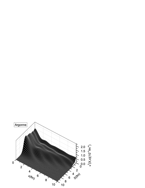
Figure 7: The pairing tensor distribution $\varkappa^{2}(X,x)$

Figure 8: The profile functions $\varkappa^{2}(X=X_{0},x)$

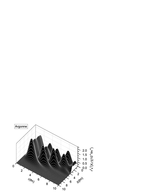
Figure 9: The probability distribution $r^{2}\varkappa^{2}(X,r)$

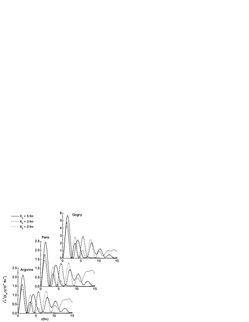
Figure 10: The profile functions $r^{2}\varkappa^{2}(X=X_{0},r)$

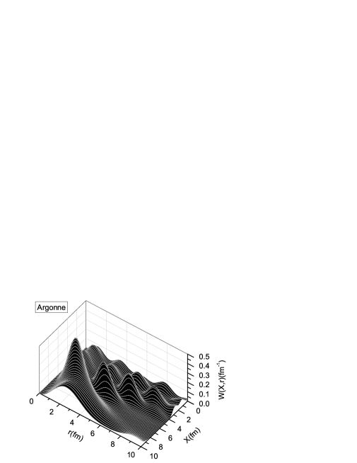
Figure 11: The locally normalized pairing tensor $W(X,r)$

Let us turn now to the correlation pairing characteristics. The total correlation lengths $\xi$ and the correlation lengths in $x$-direction $\xi_{x}$ found from Eq. (7) for each kind of force are displayed in Fig. 5 and Fig. 6, correspondingly. The curve $\xi^{\rm Arg}(X)$ is quite similar to $\xi^{\rm Par}(X)$, the difference is about 5%. Both have a minimum shifted a little from the surface, $X=L$, in direction to the free space, both have a pronounced maximum in the vicinity of $X=0$ and grow rapidly to the right from the minimum. Qualitatively, the curve $\xi^{\rm Gog}(X)$ behaves in a similar way, but the maximum value at $X=0$ is approximately two times less than those for realistic forces. The minimum of $\xi^{\rm Gog}(X)$ is also shifted from the point $X=L$, but the value of the shift is less. Such a behavior of each curve $\xi(X)$ qualitatively agrees with naive local density approximation (LDA) predictions. Indeed, inside the slab, the local Fermi momentum $k_{\mbox{\scriptsize F}}(X\simeq 0)\simeq\sqrt{2m(\mu-U_{0})}\simeq 1.4\;$fm^-1 which corresponds to big values of $\xi$ in infinite matter (see Fig. 2). The same is true at $X>8\;$fm where the local Fermi momentum vanishes. But under more detailed examination, deviations from the LDA predictions are significant. To illustrate this point, we display in Fig. 5 with a thick line, in arbitrary units, the density distribution $\rho(X)$. Within the LDA, the correlation length $\xi(X)$ should show a plateau inside the slab, just as the density does. Instead, $\xi(X)$ is decreasing rapidly with increase of $X$ till $X\simeq L$. Qualitatively, the coordinate dependence of the function $\xi(X)$ in the slab reminds us that of $\xi(R)$ in spherical nuclei found in PiSanSch . Both of them have minima at the surface region and pronounced maxima in the center. But any quantitative comparison is hardly possible since, for the problem under consideration, the properties of the two systems are essentially different. Indeed, in a spherical nucleus all particles move in a finite space limited by the nuclear surface. On the contrary, in a slab the particle motion is limited only in the $x$-direction. In the ${\bf s}$-plane, the motion is free which leads to very big values of $\xi_{s}$ in Eq. (7) and $\xi$ close to that in infinite system. As to the $\xi_{x}(X)$ function, it should be much closer to $\xi(R)$ of PiSanSch . As it is seen in Fig. 6, two curves $\xi^{\rm Arg}_{x}(X)$ and $\xi^{\rm Par}_{x}(X)$ practically coincide. Deviation of $\xi^{\rm Gog}_{x}(X)$ from the both is much less than in the case of the total correlation length. It doesn’t exceed 15%. All three curves have common minimum at $X\simeq L$, with the value of $\xi_{x}^{\min}\simeq 1.5\;$fm. It is not far from the value of $\xi^{\min}\simeq 2\;$fm found in PiSanSch for Sn isotopes. Evidently, the difference is mainly due to geometry effects. Thus, for a nuclear slab, the correlation length of pairing in the $x$-direction at the surface, calculated with realistic and semi-realistic Gogny forces, is very small, in agreement with conclusions of PiSanSch .

To visualize the pairing tensor distribution, we draw a 3-dimensional plot in Fig.7 for the $\varkappa^{2}(X,x)$ function given by Eq. (9) for the Argonne force. We see that there is a set of maxima at $x=0$, the highest one being near to the slab surface, $X\simeq L$. Fig.8 shows the profile functions $\varkappa^{2}(X=X_{0},x)$ for several values of $X_{0}$ corresponding to the maximum positions. The nearest to the surface maximum there is at $X_{0}\simeq 5\;$fm, the neighboring one, at $X_{0}\simeq 3\;$fm. There is also a pronounced maximum at $X_{0}=0$. The surface peak is very narrow, in correspondence with Fig.6. On the contrary, in the case of $X_{0}=0$ a comparatively sharp peak is accompanied by a flat base plate which results in a big value of $\xi_{x}$. The similar profile functions are drawn, in the same figure, for the Paris and Gogny force. The Paris curves are again quite similar to the Argonne ones. As to the Gogny force, the similarity takes place only at qualitative level, absolute values of $\varkappa^{2}$ being bigger than those for realistic forces. This is the result of bigger values of the gap itself for the Gogny force, as illustrated in Fig. 3. We see that $\Delta_{\mbox{\scriptsize F}}^{\rm Par}$ is a little bigger than $\Delta_{\mbox{\scriptsize F}}^{\rm Arg}$, therefore $(\varkappa^{\rm Par})^{2}$ is, on average, bigger than $(\varkappa^{\rm Arg})^{2}$. On the other side, $\Delta_{\mbox{\scriptsize F}}^{\rm Gog}$ is significantly bigger than the gap for realistic forces. As the result, $(\varkappa^{\rm Gog})^{2}$ significantly exceeds the microscopic values as well. Note that the correlation length $\xi(X)$, Eq. (6), does not depend on the magnitude of $\varkappa$, giving rise to a much smaller difference between the Gogny and realistic forces. The same is true for $\xi_{x}(X)$, Eq. (7). The surface peak dominates, to some extent, for all three kinds of forces, and this effect for realistic forces is even stronger than for Gogny force.

The $\varkappa^{2}(X,r)$ function given by Eq. (8) multiplied by $r^{2}$ gives the probability distribution of paring correlations similar to Eq. (3) in the case of the spherical symmetry. It is displayed in Fig.9, again for the Argonne force. Now the main maximum positions are shifted from $r=0$ to $r\simeq 1\div 2\;$fm due to the factor $r^{2}$. The surface maximum at $X\simeq L$ is even more pronounced than in Fig.7. To compare results obtained for different forces under consideration, we again draw the profile functions $r^{2}\varkappa^{2}(X=X_{0},r)$, see Fig.10. Again, just as in Fig.8, the Gogny force results are significantly bigger than those of realistic ones in the magnitude but are very similar in the form. Again the surface maxima dominates and again the surface enhancement is stronger for realistic forces.

Figure 12: The profile functions $W(X_{0},r)$

To make the comparison with PiSanSch more complete, we display in Fig.11 the locally normalized pairing tensor which is defined as

$$W(X,r)=\dfrac{r^{2}\varkappa^{2}(X,r)}{\int\varkappa^{2}(X,r)\;d^{3}r}\;,$$ (17)

similar to the definition (5) in spherical systems. The profile functions $W(X=X_{0},r)$ are displayed in Fig.12 which is analogous to Fig.8 and Fig.10. In this case, the Gogny force curves are close to those for realistic forces not only in the form but also in the magnitude. This is happens because the $\varkappa^{2}$ quantity comes in both the numerator and the denominator of Eq. (17), the result being almost independent of the magnitude of $\varkappa$. Absolutely similar situation occurs with calculations of the correlation lengths $\xi$ and $\xi_{x}$.

The denominator of Eq. (17),

$$p(X)=\int\varkappa^{2}(X,r)\;d^{3}r=\int\varkappa^{2}(X,x)\;dx\;,$$ (18)

gives the total probability distribution of Cooper pairs integrated over relative coordinates. Note that this quantity displayed in Fig.13, just as $P(R,r)$, Eq. (3), is not normalized to unity. Again we see that the result for the Gogny force behaves qualitatively similar to those for the realistic forces but its magnitude is significantly bigger. And for each force under consideration this quantity in the slab does not exhibit any surface enhancement. It occurred because, although the surface maximum for any force in Fig.8 is higher than the central one, the correlation length in the $x$-direction at the surface is much smaller than inside the slab that makes the integral over $x$ to be smaller. An analogous effect should take place in nuclei, too, but in this case the “geometrical” factor $R^{2}$ in Eq. (3) would help to survive to the surface enhancement in the Cooper pairs distribution if the probability $P(R,r)$, Eq. (3), is integrated over the relative coordinates.

Figure 13: The integrated Cooper pair probability distribution $p(X)$

IV Conclusion

Spatial correlation properties of nuclear pairing in a nuclear slab are studied with two realistic NN potentials, the Paris and Argonne v₁₈, and with the phenomenological Gogny D1S interaction. The results obtained with the two realistic forces agree with each other with an accuracy of about 10%. But they agree only qualitatively with those of the Gogny force. The gap value in the slab for the Gogny force exceeds that from the realistic forces by a factor about 2 , which results in rather bigger values of the anomalous density matrix $\varkappa$. Nevertheless, some of main conclusions of PiSanSch obtained for finite nuclei with the Gogny force are confirmed qualitatively, especially the dependence of the correlation length on the position of the c. m. of a Cooper pair. This quantity does not depend practically on the absolute value of $\varkappa$, only the space distribution of the pairing tensor $\varkappa^{2}(X,x)$ being important. At the surface of the slab the local value of the correlation length in the $x$-direction is very small, $\xi_{x}(X\simeq L)\simeq 1.5\;$fm, for all three kinds of the force under consideration. Inside the slab $\xi_{x}$ becomes very large, i.e. of the order of the slab width or even more. Thus, in this point our results completely confirm those of PiSanSch .

The pairing tensor $\varkappa^{2}(X,x=0)$ has several maxima, among them the ones at $X=0$ and $X\simeq L$ are most pronounced. And the one at the surface is a bit higher, especially for realistic forces. In this sense, we can speak of surface enhancement of the Cooper pair distribution. However, the total probability $p(X)$ for a pair to have the c.m. coordinate $X$, which is obtained by integrating $\varkappa^{2}(X,x)$ over relative coordinate, has no surface enhancement. Thus, the second conclusion of PiSanSch that Cooper pairs in nuclei prefer to be concentrated in the vicinity of the surface should not be drawn for a slab. We explain this with different geometrical properties of two systems under comparison, with different “surface-to-volume ratio” in a sphere and in a slab. However, all surface enhancement features found for realistic forces are qualitatively reproduced with the Gogny force. We trace this effect to the “semi-realistic” nature of the Gogny force which describes the low-energy NN-scattering in the ${}^{1}S_{0}$-channel sufficiently well. It seems reasonable to suppose that all main conclusions of PiSanSch will be confirmed qualitatively if the Gogny force in the pairing channel will be replaced by a realistic NN-potential.

This research was partially supported by the Grant NSh-3003.2008.2 of the Russian Ministry for Science and Education and by the RFBR grants 06-02-17171-a and 07-02-00553-a. Two of us (S.P. and E.S.) thank the INFN, Seczione di Catania, for hospitality.

References

- (1) M. Baldo, U. Lombardo, E.E. Saperstein, M.V. Zverev, Phys. Rep. 391, 261 (2004).
- (2) M.V. Zverev, E.E. Saperstein, Sov. J. Nucl. Phys. 42, 683 (1985).
- (3) M. Baldo, U. Lombardo, E.E. Saperstein, M.V. Zverev, Nucl. Phys. A 628, 503 (1998).
- (4) M. Baldo, U. Lombardo, E.E. Saperstein, M.V. Zverev, Phys. Lett. B459, 437 (1999).
- (5) M. Farine, P. Schuck, Phys. Lett. B459, 444 (1999).
- (6) M. Baldo, M. Farine, U. Lombardo, E.E. Saperstein, P. Schuck and M.V. Zverev, Eur. Phys. J. A 18, 17 (2003).
- (7) S.S. Pankratov, M. Baldo, U. Lombardo, E.E. Saperstein, and M.V. Zverev, Nucl. Phys. A765, 61 (2006).
- (8) S.S. Pankratov, M. Baldo, U. Lombardo, E.E. Saperstein, and M.V. Zverev, Nucl. Phys. A811, 127 (2008).
- (9) N. Pillet, N. Sandulescu and P. Schuck, Phys. Rev. C 76, 024310 (2007).
- (10) J.-F. Berger, M. Girod, and D. Gogny, Comput. Phys. Commun. 63, 365 (1991).
- (11) F. Catara, A. Insolia, E. Maglione, and A. Vitturi, Phys. Rev. C 29, 1091 (1984).
- (12) L. Ferreira, R. Liotta, C.H. Dasso, R.A. Broglia, and A. Winther, Nucl. Phys. A426, 276 (1984).
- (13) G.F. Bertsch and H. Esbensen, Ann. Phys.(NY) 209, 327 (1991).
- (14) K. Hagino, H. Sagawa, J. Carbonell, and P. Schuck, Phys. Rev. Lett. 99, 022506 (2007).
- (15) U. Lombardo and P. Schuck, Phys. Rev. C 63, 038201 (2001).
- (16) S.A. Fayans, S.V. Tolokonnikov, E.L. Trykov, and D. Zawischa, Nucl. Phys. A676, 49 (2000).
- (17) F. Barranco, R.A. Broglia, G. Colo, G. Gori, E. Vigezzi, and P.F. Bortignon, Eur. Phys. J. A 21, 57 (2004).
- (18) A.V. Avdeenkov, S.P. Kamerdzhiev, JETP Lett. 69, 715 (1999).
- (19) S. Kamerdzhiev, E.E. Saperstein, Eur. Phys. J. A 37, 333 (2008).