Non-WKB Models of the FIP Effect: Implications for Solar Coronal Heating and the Coronal Helium and Neon Abundances

Abstract

We revisit in more detail a model for element abundance fractionation in the solar chromosphere, that gives rise to the “FIP Effect” in the solar corona and wind. Elements with first ionization potential below about 10 eV, i.e. those that are predominantly ionized in the chromosphere, are enriched in the corona by a factor 3-4. We model the propagation of Alfvén waves through the chromosphere using a non-WKB treatment, and evaluate the ponderomotive force associated with these waves. Under solar conditions, this is generally pointed upwards in the chromosphere, and enhances the abundance of chromospheric ions in the corona. Our new approach captures the essentials of the solar coronal abundance anomalies, including the depletion of He relative to H, and also the putative depletion of Ne, recently discussed in the literature. We also argue that the FIP effect provides the strongest evidence to date for energy fluxes of Alfvén waves sufficient to heat the corona. However it appears that these waves must also be generated in the corona, in order to preserve the rather regular fractionation pattern without strong variations from loop to loop observed in the solar corona and slow speed solar wind.

1 Introduction

Since about 1985 it has been recognized that the composition of the solar corona and the photosphere are not the same. In the corona, the ratios of abundances of elements with first ionization potentials (FIP) less than about 10 eV relative to abundances of elements with a FIP greater than about 10 eV are about a factor of 3-4 times higher than in the photosphere. Those elements with a FIP greater than 10 eV appear to have a photospheric composition in general (with respect to hydrogen) in the corona, and the low FIP elements are enhanced in abundance there. This fractionation has recently been explained (Laming, 2004a) as being due to the ponderomotive force in the chromosphere from Alfvén waves. This is usually directed upwards, and acts on chromospheric ions, but not neutrals. Elements that are predominantly ionized in the chromosphere (low FIP elements like Al, Mg, Si, Ca, and Fe) can be enhanced in abundance as they flow up to the corona, whereas high FIP elements such as C, N, O, Ne, and Ar that are largely neutral appear essentially unaffected. The abundance of sulfur (FIP = 10.36 eV) is between photospheric and coronal.

It was recognized very early that the most plausible site for FIP fractionation was the chromosphere, where low FIP elements are generally ionized and where high FIP elements are at least partially neutral. Henoux (1995, 1998) reviewed the early models. Those which rely on ion-neutral separation by diffusion in magnetic fields, in temperature gradients, or in upward plasma flows suffer from problems of the speed of the process (diffusion is inherently slow) or the choice of boundary conditions. Realistic FIP effect models must include some form of external force that acts upon the plasma ions but not upon the neutrals. The first effort along these lines (Antiochos 1994) considered the cross-B thermoelectric electric field associated with the downward heat flux carried by electrons which gives rise to chromospheric evaporation. This draws ions into the flux tube, enhancing their abundance over neutrals. The absence of a FIP effect in coronal holes arises naturally, but in coronal regions where FIP fractionation occurs, a mass dependence is predicted, which is not observed.

Henoux & Somov (1992) proposed that cross-B pressure gradients arising in current carrying loops could enhance the ion abundance by a “pinch” force. Azimuthal motions of the partially ionized photosphere at flux tube boundaries generate a system of currents flowing in opposite directions, such that the azimuthal component of the field vanishes at infinity. Details of the fractionation (mass dependence, degree, etc) remain to be worked out, but it is thought to begin just above the temperature minimum region at about 4000 K, and continue until temperatures where all elements are ionized. More recent suggestions have been that chromospheric ions, but not neutrals, are heated by either reconnection events (Arge & Mullan 1998), or by waves that can penetrate down to loop footpoints from the corona (Schwadron, Fisk & Zurbuchen 1999). Strengths and weaknesses of these two models are discussed in some detail by Laming (2004). For the time being we comment that although both models seem capable of producing mass independent fractionation of about the right degree, they, in common with the others mentioned above, only predict positive FIP effects. In these models there is no possibility of an “inverse FIP” effect such as seen in the coronae of active stars (see e.g. Feldman & Laming 2000, Laming 2004 and references therein).

This consideration led Laming (2004) to consider the action of ponderomotive forces due to Alfvén waves propagating up through the chromosphere and either transmitting into or being reflected from coronal loops. This force can in principle be either upward or downward and is given approximately by (see derivation in Appendix A)

$$F={q^{2}\over 4m\left(\Omega^{2}-\omega^{2}\right)}{\partial\delta E_{\perp}^{2}\over\partial z}$$ (1)

where $\Omega$ and $\omega$ are the particle cyclotron frequency and the wave frequency respectively, $q$ and $m$ the charge and mass, and $E_{\perp}$ is the wave peak transverse electric field. The dependence on the Alfvén speed, $V_{A}$, means that the ponderomotive force is usually strongest at the top of the chromosphere. The ponderomotive acceleration, $F/m$, is independent of the ion mass, leading to the essentially mass independent fractionation that is observed. Using an analytic model solar loop from Hollweg (1984), upward ponderomotive forces on ions are much more common in solar conditions, and for typical density gradients in the chromosphere can be larger than the gravitational force downward. The magnitude of the FIP fractionation is dictated by the resonant properties of the coronal loop and the corresponding wave energy density. Large loops with resonant frequencies similar to the chromospheric period of 200-300 seconds admit strong Alfvén wave fluxes with correspondingly large FIP fractionation. Open field lines, or coronal holes, with formally infinite wave periods or unresolved fine structures (i.e. the chromosphere and lower transition region away from coronal loop footpoints, Feldman 1983, 1987) with much shorter wave periods do not have much Alfvén wave transmission into them and so would have very low FIP fractionation, as observed. Using model chromospheres from Vernazza, Avrett, & Loeser (1981), most of the FIP fractionation is found to occur at the top of the chromosphere at altitudes with strong density gradients near the plateau regions, where low FIP elements are essentially completely ionized and high FIP elements are typically at least 50% ionized. The Laming (2004) model thus comes about as a natural extension of existing work on Alfvén wave propagation in the solar atmosphere with essentially no extra physics required.

In this paper we revisit the Laming (2004a) model using a numerical treatment of Alfvén wave propagation in a coronal loop rooted in the chromosphere at each footpoint. Section 2 describes this model and the improvements over Laming (2004a) with a series of illustrative examples. Section 3 gives a more complete tabulation of the FIP fractionation expected in a variety of elements, and section 4 gives some discussion of the implications of the new models, both for the solar coronal abundances of helium and neon, and for MHD wave origin and propagation in the solar atmosphere, before section 5 concludes.

2 Ponderomotive Driving of the FIP Effect

2.1 Introduction and Formalism

Laming (2004) used a WKB approximation to treat the case of strong transmission of Alfvén waves into a coronal loop, and hence evaluate the FIP fractionation. Here we have extend this work to a non-WKB treatment. The procedure follows that described in detail by Cranmer & van Ballegooijen (2005), but applied to closed rather than open magnetic field structures. The transport equations are (see Appendix B for a derivation)

$${\partial I_{\pm}\over\partial t}+\left(u\pm V_{A}\right){\partial I_{\pm}\over\partial z}=\left(u\pm V_{A}\right)\left({I_{\pm}\over 4H_{D}}+{I_{\mp}\over 2H_{A}}\right),$$ (2)

where $I_{\pm}=\delta v\pm\delta B/\sqrt{4\pi\rho}$ are the Elsässer variables for inward and outward propagating Alfvén waves respectively. The Alfvén speed is $V_{A}$, the upward flow speed in $u$ and the density is $\rho$. The signed scale heights are $H_{D}=\rho/\left(\partial\rho/\partial z\right)$ and $H_{A}=V_{A}/\left(\partial V_{A}/\partial z\right)$. In the solar chromosphere and in closed loops we may take $u<<V_{A}$.

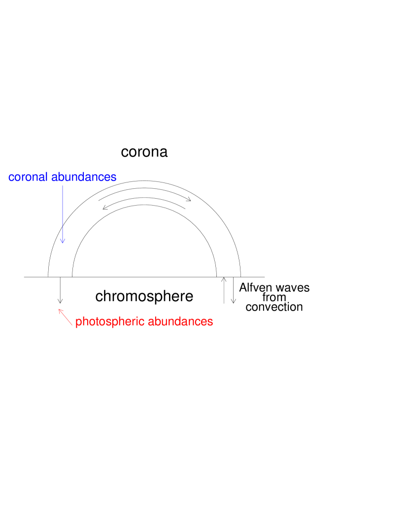
Figure 2: Cartoon illustrating the model. Alfvén waves are incident on the coronal loop from below on the right hand side. Waves are either transmitted into the loop or reflected back down again. Waves in the coronal loop bounce back and forth, with some leakage at each footpoint. The magnetic field is taken to be uniform in the coronal section of the loop (illustrated), while it varies according to Figure 1 within the chromosphere (not shown on this figure).

We use the same chromospheric model as before in Laming (2004), but this time also embedding it in a 2D force-free magnetic field computed from formulae given in Athay (1981), and shown in Figure 1. We take a scale here of 1 unit to 1,000 km, and place the bottom of the plot at 500km altitude in the chromosphere. The region where the plasma beta (ratio of gas pressure to magnetic pressure) equals unity is taken at 650 km altitude, or at $y=0.15$ in the figure. This region is where upcoming acoustic waves from the convection zone can convert to Alfvén waves by mode or parametric conversion, or where downgoing Alfvén waves can convert back to acoustic waves. We adopt an altitude of 650 km as the boundary of our simulations where Alfvén waves are launched upwards. We consider a loop model similar to that of Hollweg (1984), the coronal portion of which is illustrated in Figure 2. Waves from beneath impinge on the right hand side chromosphere-corona boundary and are either reflected back down, or transmitted into the loop. Waves in the loop section bounce back and forth, with a small probability of leaking back into the chromosphere at either end. The magnetic field in the coronal loop section is uniform, and is simply the extension of chromospheric force-free field into the corona. In the current work, the non-uniformity of the magnetic field in the low chromosphere has no effect on the FIP effect, since the fractionation in this work appears towards the top of the chromosphere where the magnetic field is almost parallel. The loop density is similarly extrapolated, but with a density scale height taken here to be equal to the loop length. All models presented here assume waves propagating up the $y$-axis at $x=0$.

Equations (2) are integrated from a starting point in the left hand side chromosphere (hereafter chromosphere “A”) where Alfv’en waves leak down into the chromosphere, back through the corona to the right hand side (chromosphere “B”) where waves are fed up from below. In this way the reflection and transmission of Alfvén waves at the loop footpoints and elsewhere is naturally reconstructed. The velocity and magnetic field perturbations are calculated from

$$\delta v ={I_{+}+I_{-}\over 2}$$ (3)

$${\delta B\over\sqrt{4\pi\rho}} ={I_{+}-I_{-}\over 2}.$$ (4)

The wave energy density and positive and negative going energy fluxes are

$$U ={\rho\delta v^{2}\over 2}+{\delta B^{2}\over 8\pi}={\rho\over 4}\left(I_{+}^{2}+I_{-}^{2}\right)$$ (5)

$$F_{+} ={\rho\over 4}I_{+}^{2}V_{A}$$ (6)

$$F_{-} ={\rho\over 4}I_{-}^{2}V_{A},$$ (7)

and the wave peak electric field appearing in equation (1) is

$$\delta E_{\perp}^{2}={B^{2}\over 2c^{2}}\left(I_{+}^{2}+I_{-}^{2}\right).$$ (8)

Given the ponderomotive acceleration from equation (1), the FIP fractionations are calculated in a similar manner to Laming (2004a), but with one important modification. In the momentum equations (10) and (11) of Laming (2004a), we add the motion in the wave to the ion and neutral partial pressures, so that $P_{s,i,n}=\left(k_{\rm B}T/m_{s}+v_{turb}^{2}+v_{wave}^{2}\right)\rho_{s,i,n}/2$ where the first two terms in parentheses represent the ion thermal velocity and the microturbulent velocity in the model chromosphere, and the third term represents the motion of the ion in the Alfvén wave. In true collisionless plasma, neutrals would not respond to the wave. However the solar chromosphere is sufficiently collisional that neutrals move with the ions in the wave motion (e.g. Vranjes et al., 2008) for wave frequencies well below the charge exchange rate that couples neutrals and ions, and so neutrals require the same form for their partial pressure as the ions. Following the derivation through, writing $\nu_{s,n}\partial P_{s,i}/\partial z+\nu_{s,i}\partial P_{s,n}/\partial z$ from equations (10) and (11) in Laming (2004a) (with the ponderomotive term in $\partial\rho_{s,i}/\partial z\rightarrow 0$, i.e. $b=0$) we find

$${\partial\over\partial z}\left[{\rho_{s}\over 2}\left({k_{\rm B}T\over m_{s}}+v_{turb}^{2}+v_{wave}^{2}\right)\right]+\rho_{s}\left[g+\nu_{eff}\left(u_{s}-u\right)\right]+\rho_{s}a\xi_{s}\nu_{eff}/\nu_{si}=0$$ (9)

where $\nu_{eff}=\nu_{s,i}\nu_{s,n}/\left[\xi_{s}\nu_{s,n}+\left(1-\xi_{s}\right)\nu_{s,i}\right]$, with $\xi_{s}$ being the ionization fraction of element $s$, and $\nu_{s,i}$ and $\nu_{s,n}$ the collision rates of ions and neutrals respectively of element $s$ with the ambient gas, and $a$ the ponderomotive acceleration. This leads to

$${\rho_{s}\left(z_{u}\right)\over\rho_{s}\left(z_{l}\right)}={v_{s}\left(z_{l}\right)^{2}\over v_{s}\left(z_{u}\right)^{2}}\exp\left(2\int_{z_{l}}^{z_{u}}{-g-\nu_{eff}\left(u_{s}-u\right)+\xi_{s}a\nu_{eff}/\nu_{s,i}\over v_{s}^{2}}dz\right)$$ (10)

where $v_{s}^{2}=kT/m_{s}+v_{turb}^{2}+v_{wave}^{2}$. We argue that in the absence of the ponderomotive acceleration $a$, the effect of turbulence should be to fully mix the element composition. Thus we choose $u_{s}$ in equation (7) such that

$${v_{s}\left(z_{l}\right)^{2}\over v_{s}\left(z_{u}\right)^{2}}\exp\left(2\int_{z_{l}}^{z_{u}}{-g-\nu_{eff}\left(u_{s}-u\right)\over v_{s}^{2}}dz\right)=1$$ (11)

to yield the fractionation by the ponderomotive force as

$${\rho_{s}\left(z_{u}\right)\over\rho_{s}\left(z_{l}\right)}=\exp\left(2\int_{z_{l}}^{z_{u}}{\xi_{s}a\nu_{eff}/\nu_{s,i}\over v_{s}^{2}}dz\right).$$ (12)

As mentioned previously (Laming, 2004a), the solar chromosphere is undoubtedly more active and dynamic than represented by equations (6-9). However this choice allows us to model a chromosphere which in the absence of Alfvén waves is completely mixed, presumably by hydrodynamic turbulence, and upon which the ponderomotive force acts to selectively accelerate chromospheric ions. Chromospheric simulations excluding turbulence find huge (and unobserved) variations in various coronal element abundances due to ambipolar and thermal diffusion (Killie & Lie-Svendson, 2007). It would appear that such abundance variations are unavoidable in the situation that the chromosphere remains undisturbed for a sufficient length of time (days to weeks in the case of Killie & Lie-Svendson, 2007). We argue that hydrodynamic turbulence acts on timescales much shorter than this (but still longer than that required to establish the FIP effect) to leave a fully mixed chromosphere in the absence of ponderomotive forces. We model the ponderomotive acceleration as acting only on the chromospheric ions, since the ponderomotive acceleration divided by the flow velocity $a/u\sim 10-1000$ s^-1 is much greater than the charge exchange rate (of order 1 s^-1). This rate should also be sufficiently greater than the turbulent mixing rate discussed above.

We also use a more recent chromospheric model (model C7 in Avrett & Loeser, 2008), introduced as an update to the older VALC model (Vernazza, Avrett, & Loeser, 1981) used previously in Laming (2004a). We continue to evaluate photoionization rates using incident spectra based on Vernazza & Reeves (1978) with the extensions and modifications outlined in Laming (2004a). In most cases, the “very active region” spectrum is used, being the most consistent with the underlying chromospheric model.

2.2 A Loop On Resonance

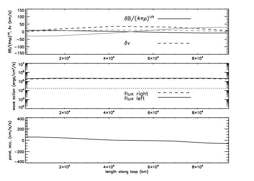
Figure 3: Coronal section of loop, length 100,000 km, magnetic field 9.9 G, (half wavelength long) showing from top: Elsässer variables in km s^-1 ($\delta B/\sqrt{4\pi\rho}$ solid lines, $\delta v$ dashed lines), with black lines for real parts and gray lines for imaginary parts. The loop is approximately half a wavelength long. Middle; wave energy fluxes in ergs cm^-2 s^-1, the thin solid line shows the difference in energy fluxes divided by the magnetic field strength and should be a horizontal line if energy is properly conserved. Bottom, the ponderomotive acceleration in cm s^-2. Positive acceleration means positive along the $z$ axis, which is upwards pointing near $z=0$ and downwards near $z=100,000$.

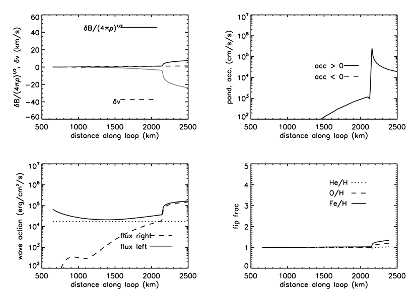
Figure 4: Same as figure 3 giving the first three panels for the left hand chromosphere “A”, where waves leak down from the corona. The extra bottom right panel shows the FIP fractionation for Fe, O, and He, relative to H.

In the following, Figures 3, 4, and 5 illustrate the solutions for a loop 100,000 km long, with coronal magnetic field $B=9.9$ G. This yields a wavelength for 3 minute period waves approximately the same as twice the loop length, and therefore such waves can be transmitted into the coronal loop section from the chromosphere. We concentrate on 3 minute waves since unlike 5 minutes waves, these require no special conditions to propagate up into the corona (de Pontieu et al., 2005). Figure 3 shows the coronal section of the loop. From top to bottom the three panels give the amplitudes of $\delta v$ and $\delta B/\sqrt{4\pi\rho}$ in units of km s^-1. Real and imaginary parts are given as black and gray lines respectively, with $\delta B/\sqrt{4\pi\rho}$ and $\delta v$ given by solid and dashed line respectively. The wave amplitude has been chosen to be $\sim 30$ km s^-1 in the corona, giving a typical spectral line FWHM consistent with observations (e.g. McIntosh et al., 2008). The second panel gives the wave actions (energy fluxes) for the left going (solid) and right going (dashed) lines, and their difference divided by the magnetic field as a dotted line, in arbitrary units. This last quantity should be a straight horizontal line if energy is properly conserved in the calculation. The third panel gives the ponderomotive acceleration, in cm s^-2. Throughout the coronal section of the loop, it is significantly lower than the gravitational acceleration. Solid lines indicate positive, i.e. right going, and dashed lines indicate left going accelerations. The oscillation amplitude has been chosen to give mass motions within observational constraints (Chae et al., 1998; McIntosh et al., 2008), as measured from line profiles.

Figure 4 shows the same three plots for the left hand side chromosphere “A”, where waves leak down from the corona, together with a fourth panel showing the degree of fractionation for the abundance ratios Fe/H, O/H, and He/H. The ponderomotive acceleration in the chromosphere is much larger than in the corona, especially towards the top. The most significant fractionation occurs here, increasing Fe/H in this case by a factor of 1.4 over photospheric values, O/H by a factor of around 1.25, with He/H remaining nearly unchanged.

Finally Figure 5 shows the same four panels for the chromosphere “B” on the right hand side, where the upgoing Alfvén waves originate. The ponderomotive acceleration is still pointed upwards (though is negative in the coordinate system used here), giving the same FIP fractionations as before. In exact resonance, the chromospheric ponderomotive force behaves the same as at the opposite footpoint already shown in Figure 4.

2.3 A Loop Off Resonance

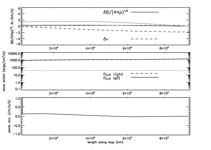
Figure 6: Coronal section of loop, length 100,000 km, magnetic field 19.8 G, showing from top: Elsässer variables in km s^-1 ($\delta B/\sqrt{4\pi\rho}$ solid lines, $\delta v$ dashed lines), with black lines for real parts and gray lines for imaginary parts. The loop is now a quarter wavelength long and reflects most Alfvén waves incident from below, and consequently has much smaller nonthermal motions than the previous resonant case. Middle; wave energy fluxes in ergs cm^-2 s^-1. Bottom, the ponderomotive acceleration in cm s^-2.

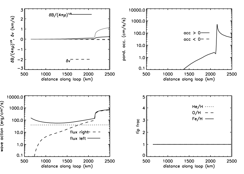
Figure 7: Same as figure 6 giving the first three panels for the left hand chromosphere “A”, where waves leak down from the corona. The extra bottom right panel shows the FIP fractionation for Fe, O, and He, relative to H. In the case of a loop off resonance, no waves are transmitted through to chromosphere “A”, and no fractionation occurs.

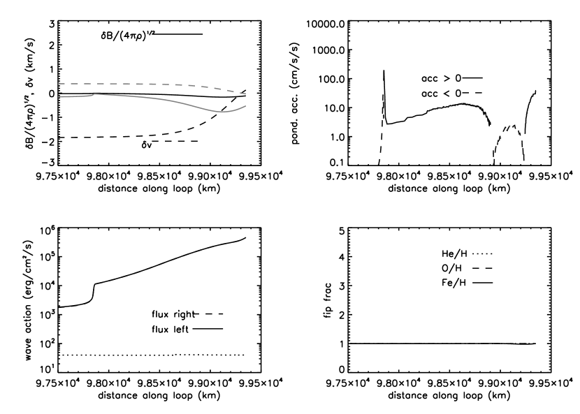
Figure 8: Same as figure 7 for the right hand side chromosphere “B”, where Alfvén waves are launched up from the convection zone. Almost complete reflection of Alfvén waves occurs from the loop footpoint, leading to no fractionation.

Figures 6, 7 and 8 show the same variables as before, but for a loop 100,000 km long and with magnetic field $B=19.8$ G. Now the loop is a quarter wavelength long, and almost complete reflection of the incident Alfvén waves on the right hand side takes place. The simulation has been normalized so that the incident Alfvén wave flux coming up from the chromosphere is about the same as for the on resonance case. Figure 6 shows that the coronal loop oscillation is now much weaker than before, by about a factor 20. In the left hand chromosphere “A” (Figure 7) negligible Alfvén wave flux leaks through and no FIP fractionation occurs. In the right hand chromosphere “B” (Figure 8), the behavior is quite different to the previous case. The ponderomotive force is now downwards pointing for most heights in the chromosphere, and it is still very small, also giving essentially no FIP fractionation. The downward directed ponderomotive force might be of interest in cases where the turbulence is stronger. As reviewed in Laming (2004a), the coronae of various active stars exhibit an inverse FIP effect, where the low FIPs are depleted in the corona instead of being enhanced. The reversal of the ponderomotive force under these conditions is a plausible mechanism for such abundance anomalies.

2.4 Loops with Stronger Turbulence

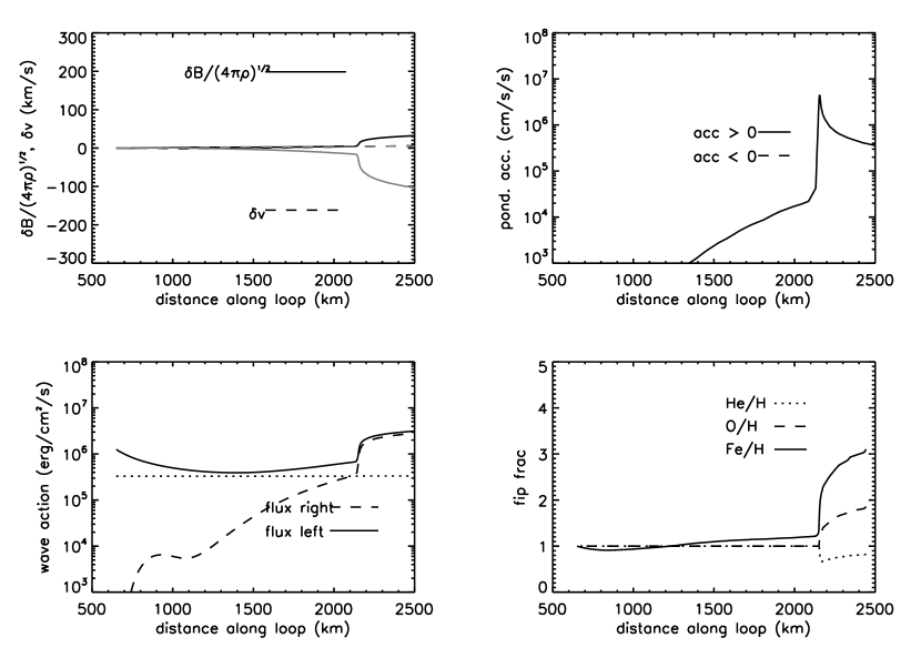
Figure 9: Same as figure 4 (on resonance case) giving the first three panels for the left hand chromosphere “A”, where waves leak down from the corona. The extra bottom right panel shows the FIP fractionation for Fe, O, and He, relative to H. The wave energy flux has been increased by a factor 20, leading to stronger coronal nonthermal motions, and stronger fractionation. Helium is now depleted in the corona relative to the chromosphere.

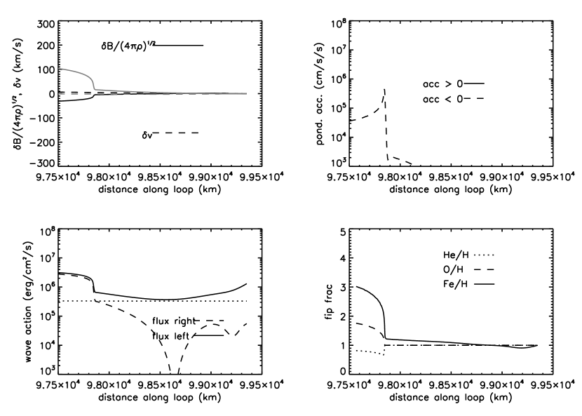
Figure 10: Same as figure 5 (on resonance case) for the right hand side chromosphere “B”, where Alfvén waves are launched up from the convection zone. The wave energy flux has been increased by a factor 20, leading to stronger coronal nonthermal motions, and stronger fractionation.

The first case above was designed to give a coronal nonthermal mass motion within observational limits, i.e. a root mean square $\delta v\simeq 30$ km s^-1. The upgoing energy flux of Alfvén waves at the loop footpoint is $\sim 10^{5}$ ergs cm^-2 s^-1, and is insufficient to power the coronal radiation power loss by one to two orders of magnitude. In this subsection we consider the same loop as in the first case, but with an Alfvén wave upward energy flux of about $2\times 10^{6}$ ergs cm^-2 s^-1; sufficient to power radiation from a 100,000 km loop with a density of $10^{8}-10^{9}$ cm^-3. The predicted nonthermal mass motions in the corona are now unphysically high, in excess of 100 km s^-1, unless we are able to argue that only a small region of the corona oscillates with this speed. We discuss this further in subsection 4.1. This is less of a problem in the transition region where the “classical” transition region that connects a coronal loop with the chromosphere has only recently been identified in observations (Peter, 2001), being otherwise masked by “unresolved fine structures” (Feldman, 1983, 1987). Peter (2001) in fact observed nonthermal line broadening in what he interprets as the “classical” transition region approaching the values modeled in this section, and suggests that they arise from the passage of an Alfvén wave with sufficient energy flux to heat the corona. In this strong wave field, the behavior of the FIP fractionation is now subtly different, as shown in Figures 9 and 10 for the left and right hand side chromospheres (“A” and “B”) respectively. On each side, Fe is somewhat more enhanced than in the previous case, at 3 - 3.3. O has a FIP fractionation of about 1.7-1.8, similar to before, but He/H is now at about 0.8 of its photospheric value.

This new behavior can be understood with reference to equation 5, and the denominator in the integral, $v_{s}^{2}=kT/m_{s}+v_{turb}^{2}+v_{wave}^{2}$. In the case that the first two terms in $v_{s}^{2}$ dominate, i.e. weak Alfvén turbulence, all elements (high FIPs as well as low FIPs) are fractionated positive to H because H has the largest thermal velocity in the denominator. When the Alfvénic velocity dominates, the fractionation changes and is determined solely by the numerator in the integral. In this case the element that stays neutral the longest, He, as expected, has the lowest abundance in the corona, being depleted with respect to H. This occurs because H experiences a stronger ponderomotive enhancement. O/H is unchanged, again as expected because O and H have very similar ionization potentials and their ionization structures are locked by charge exchange reactions between them. Fe remains fractionated with respect to H, by a similar amount as before. The inclusion of the Alfvén turbulence in $v_{s}$ leads to a natural saturation of the FIP effect, at about the level observed. Thus for a wide range of turbulence levels, and FIP effect of around 3 should be expected.

The decrease in He/H is especially interesting. It might be relevant to the He abundance in the solar wind, of around 4-5% (e.g. Aellig et al., 2001; Kasper et al., 2007) compared with a photospheric abundance of 8%, also seen in coronal holes and quiet solar corona (Laming & Feldman, 2001, 2003), and is discussed further below.

3 More Realistic Examples

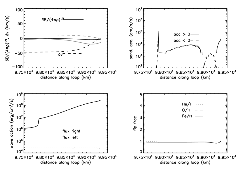
Figure 11: Same as figure 8 (off resonance case) for the right hand side chromosphere “B”, where Alfvén waves are launched up from the convection zone. The wave energy flux has been increased by a factor 20, leading to stronger coronal nonthermal motions, and stronger fractionation. Waves are now reflected, and a small inverse FIP effect results.

We put three Alfvén waves with angular frequencies 0.025, 0.022, and 0.016 rad s^-1, with relative intensities 1:0.5:0.25 in the left hand chromosphere designed to match the network power spectrum displayed in Figure 1 of Muglach (2003). The loop is 100,000 km long as before, with a magnetic field of 7.1 G, which puts the 0.025 rad $s^{-1}$ on resonance. In the first case, FIP fractionations are computed for the left hand chromosphere “A”, using the very active region spectrum of Vernazza & Reeves (1978), and are given in Table 1. This is the region where waves leak into the chromosphere from the corona before being reflected back up again, and should give FIP fractionation. The corresponding model is shown in Figure 11. There are three important differences from the tabulation given previously (Table 2 in Laming, 2004a). The first is that with increasing wave energy flux, the FIP fractionations now appear to saturate at levels corresponding to a fractionation of low FIP elements overabundant with respect to high FIP elements by a factor of about 3, and does not increase without limit. This arises from the inclusion of the term in $v_{wave}^{2}$ in the ion and neutral partial pressures discussed above, and means that for a wide range of turbulent energy densities, similar fractionated abundances should result. The other new features, already mentioned briefly above, are the depletion in the He abundance, and at higher energy fluxes also the Ne abundance relative to H. These also stem from the modification to the partial pressures.

These new calculations are compared in Table 1 with observations from Zurbuchen et al. (2002), Bryans et al. (2008) and Giammanco et al. (2008). Zurbuchen et al. (2002) give abundances measured in the slow speed solar wind during 1997/8 relative to O, relative to photospheric abundances given by Grevesse & Sauval (1998). Bryans et al. (2008) give abundances observed spectroscopically in a region of quiet solar corona, again tabulated relative to the photospheric composition of Grevesse & Sauval (1998), with small modifications by Feldman & Laming (2000). With the exceptions of Mg and K, the calculated abundances agree well with those observed for a wave energy flux between one and four times that shown in Figure 11, both for the elements that are depleted, like He and Ne, and for those enriched. We predict stronger fractionation in Mg than is in fact observed, and stronger than in Laming (2004a). The reason for this has been tracked to the use of the newer chromospheric model from Avrett & Loeser (2008), where H retains a higher degree of ionization lower in the chromosphere than in the previous VAL models. This then in turn renders the ionization of Mg probably spuriously high because of charge transfer ionization with the ambient protons. The difference in ionization fraction between 0.99 and 0.95 makes a considerable impact on the fractionations that result. Other low FIP elements, Si, and Fe, do not have charge transfer ionization rates tabulated by Kingdon & Ferland (1996), and so are unaffected by this change. The cause of the discrepancy for K is less clear. Like Na, K is very highly ionized throughout the chromosphere due to its very low FIP, and should be expected to fractionate strongly, though Bryans et al. (2008) do comment that their analysis only includes one line of K IX.

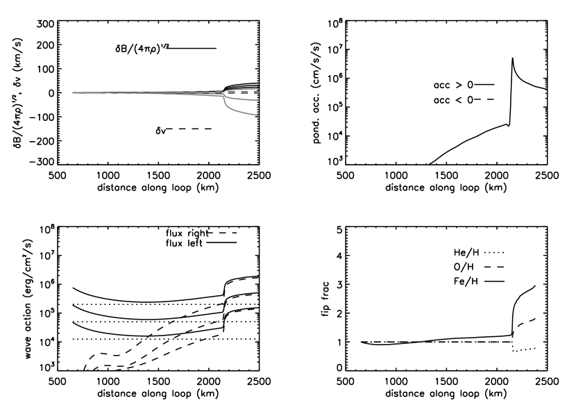
Figure 12: Same as figure 9 giving the first three panels for the left hand chromosphere “A”, where waves leak down from the corona. The extra bottom right panel shows the FIP fractionation for Fe, O, and He, relative to H. Three wave frequencies are now introduced to simulate more nearly a realistic chromospheric power spectrum.

The results of the calculation for the right hand side chromosphere “B” are given in Figure 12. The loop model chosen is resonant with the 0.025 angular frequency wave, and this is the component transmitted into the corona. However the FIP fractionation is significantly reduced by the presence of the other wave frequencies which are reflected from the corona. In the right hand chromosphere “B” the weaker components on the left are now the strongest. This does not produce much change in the ponderomotive acceleration, but increases the term $v_{wave}^{2}$ in the denominator of the integrand in equation 6, thereby reducing the fractionation. A wave source in the chromosphere is unlikely to be monochromatic, and so this situation of partial transmission and partial reflection with the reduced FIP fractionation will be ubiquitous in the solar atmosphere. This does not agree with observations, for which chromosphere “A” is a much better match. We therefore argue that if the FIP effect is due to the ponderomotive force of Alfvén waves in the chromosphere, these must have a source in the corona. We return to this thought in subsection 4.1.

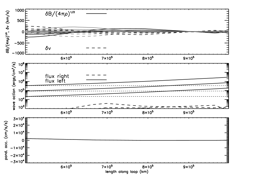
Figure 14: Coronal section of open field region up to 500,000 km altitude, showing from top: Elsässer variables in km s^-1 ($\delta B/\sqrt{4\pi\rho}$ solid lines, $\delta v$ dashed lines), with black lines for real parts and gray lines for imaginary parts. Middle; wave energy fluxes in ergs cm^-2 s^-1. Bottom, the ponderomotive acceleration in cm s^-2.

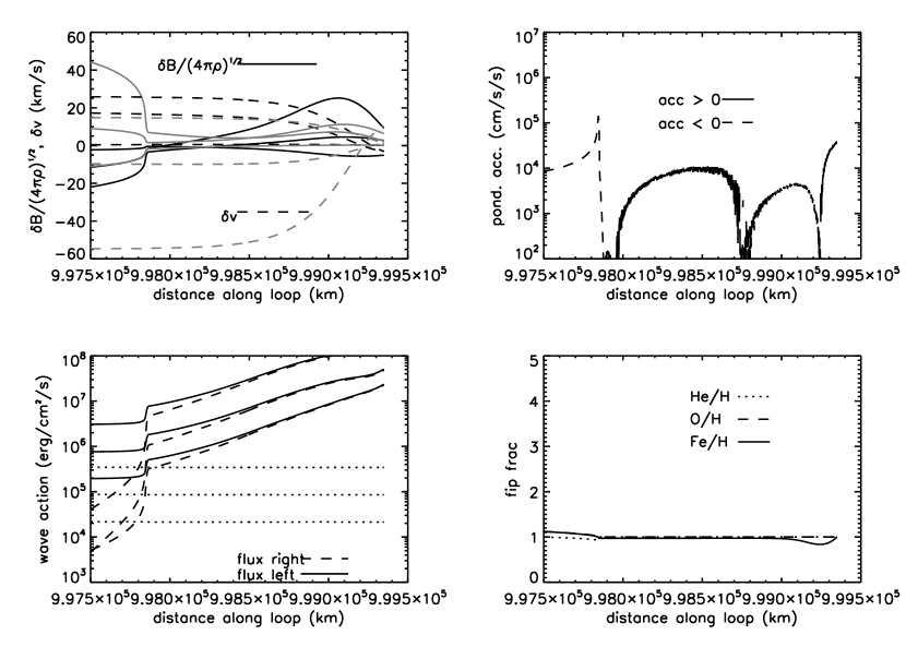
Figure 15: Same as figure 11 for the right hand side chromosphere “B”, where Alfvén waves are launched up from the convection zone into an open field region. The FIP fractionations are evaluated with an incident coronal hole spectrum, as opposed to that for an active region, and show the absence of strong fractionation consistent with observations of the fast solar wind and coronal holes.

Although this calculation has been done for a closed loop, we expect that this chromospheric wave pattern will also arise at the footpoint of an open field line in a coronal hole. In fact the character of our chromospheric solution matches well with that found in the open field case by Cranmer & van Ballegooijen (2005), subsequently shown in Cranmer et al. (2007) to exhibit FIP fractionation similar to that observed in the fast solar wind. We emphasize this point by showing in Figures 14 and 15 the coronal and chromospheric portions of an open field flux tube. In this case we start the integration at an altitude of $5\times 10^{5}$ km with purely outgoing waves, and work back to the solar surface. This restricts us to the region where the solar wind outflow speed is still much lower than the Alfvén speed, in keeping with our assumption of $u<<V_{A}$ above. We take magnetic field from Banaskiewicz et al. (1998), modified by Cranmer & van Ballegooijen (2005), and choose a density scale height to match the observed and modeled density profiles in Laming (2004b). Figure 14 shows $\delta v$ and $\delta B/\sqrt{4\pi\rho}$, chosen to match the observational and modeling constraints in Cranmer & van Ballegooijen (2005). Figure 15 shows the extension of these variables into chromosphere “B”, in a similar manner to the previous figures. While there is much more to be said about the wave properties in open field lines, the important point to be made here is that the ponderomotive force naturally produces a very small fractionation in this geometry. This is consistent with observed abundances in the fast solar wind (Zurbuchen et al., 2002) and in coronal holes (Feldman et al., 1998). A tabulation of coronal hole fractionations is given in Table 2, in a similar format to that in Table 1, using the coronal hole incident spectrum of Vernazza & Reeves (1978).

4 Discussion

4.1 Alfvén Wave Energy Fluxes

It appears from the forgoing that the abundance anomalies observed in various regions of the solar corona may yield inferences on the energy fluxes of Alfvén waves in the chromosphere. Our initial considerations then imply that wave energy fluxes sufficient to heat the solar corona or accelerate the solar wind are necessary to produce the correct fractionation. Energy fluxes observed in slow mode and fast mode waves are not sufficient to heat the solar corona (Erdélyi & Fedun, 2007). The detection of Alfvén waves, the favored mode for transporting energy to the solar corona, is much harder, since they are incompressible and can only be revealed through Doppler shifts or motions, which become hard to see in inhomogeneous conditions where Alfvén waves on neighboring flux surfaces can propagate at different speeds and lose phase coherence. However Tomczyk et al. (2007) claim the detection of Alfvén waves in the solar corona, albeit with insufficient energy flux to heat the corona. van Doorsselaere et al. (2008) argue that the detected waves are in fact kink mode waves, for the reasons suggested above. de Pontieu et al. (2007) observe transverse waves in the chromosphere, which they argue should be interpreted as Alfvén waves in the absence of a chromospheric waveguide. However these waves are inferred from the observed oscillations of spicules, which clearly have radial structure. The energy flux detected by these authors $\sim 10^{5}$ ergs cm^-2 s^-1 is close to being sufficient to heat the solar corona or accelerate the solar wind.

In this paper we argue that the FIP effect is due to the ponderomotive force associated with transverse waves in the chromosphere. Longitudinal MHD waves do not generate electric field. In order to generate the observed FIP fractionation, the energy fluxes associated with these waves need to be of order $10^{6}-10^{7}$ ergs cm^-2 s^-1, much closer to those required for coronal heating. It is clear that FIP fractionation is associated with the transmission of waves between the chromosphere and the corona, and correspondingly we argue that the required transverse waves should be identified as Alfvén waves to meet this condition. The fast mode totally internally reflects somewhere in the transition region or low corona (Schwartz & Leroy 1982, Leroy & Schwartz 1982).

The nonthermal mass motions predicted in the coronal section of this loop are higher than observed. In the transition region, this is not necessarily a problem since ample evidence exists to show that the “classical” transition regions of coronal loops are rarely observed, being masked as they are by a population of smaller “unresolved fine structures” (Feldman, 1983, 1987; Peter, 2001). In the corona, this may also be true if the heating occurs in thin filament or shells as in Alfvén resonance models (e.g. Terradas et al., 2008) while the rest of the emitting loop undergoes much slower oscillations. Another possibility might be the generation of turbulence following coronal reconnection events associated with nanoflares (Dahlburg et al., 2005). In each case it is likely that the turbulence would actually be produced in the coronal section of the loop, not in the chromosphere, and will also be in resonance with the loop. This also appears to be the conclusion to be drawn from section 3. Chromosphere “A” where waves leak down from the corona before being reflected back again gives stronger and more consistent FIP fractionations for a wide variety of wave spectra than chromosphere “B”, where waves are incident upwards on the loop from the chromosphere below. We therefore argue that the FIP effect is more likely to arise with a coronal source of Alfvén waves, rather than a chromospheric source as originally conceived in Laming (2004a), and that this inference will constrain the means by which the corona may be heated.

4.2 Helium and Neon in the Solar Corona

The fractionations computed in this paper differ from those in Laming (2004a) in three notable ways. First, as the turbulent energy density increases, the fractionation does not increase without limit but saturates at values broadly consistent with those observed. This is due to a refinement in our formalism discussed above, where the wave oscillation velocity is included in the ion and neutral partial pressures in equation 3.

The second is that at high turbulence levels, He becomes significantly depleted relative to H. Comparing Tables 1 and 2, we find a stronger depletion in the coronal loop, representative of the slow speed solar wind, than we would in a coronal hole, the source of the fast wind. The abundance ratio He/H in the fast solar wind is fairly constant at about 5% (Aellig et al., 2001; Zurbuchen et al., 2002), or a depletion of 0.59 from the photospheric value of 8.5%. He/H in the slow speed solar is lower, and generally more variable. Aellig et al. (2001) and Kasper et al. (2007) find He/H varying with wind speed, with these variations being more pronounced at solar minimum, where He/H $\sim 1\%$ for speeds below 300 km s^-1, approaching 4.5% for speeds above 500 km s^-1. At solar maximum, He/H is always in the range 3.5 - 5%. Kasper et al. (2007) also find a dependence on heliographic latitude during periods of solar minimum, with lower He/H being found closer to the heliographic equator. Table 1 gives values of He/H down to about 3.5%. Overall though, our modeled values for the abundance ratio He/H are very encouragingly consistent with observations, lending confidence to our approach.

The third, and most controversial new feature is the similar depletion predicted for Ne. This was originally suggested by Drake & Testa (2005) from a survey of the Ne/O abundance ratio in a sample of late-type stellar coronae, as a solution to the problem in helioseismology presented by the reduction in the solar photospheric abundance of O (see Caffau et al., 2008, and references therein). Specifically, (Basu & Antia, 2004) the depth of the solar convection zone demands a metallicity higher than that coming from the standard solar composition, with the O abundance revised downwards by nearly a factor of 1.5 (Asplund et al., 2004) from Grevesse & Sauval (1998). Ne, having no photospheric lines on which to base an abundance measurement, was suggested as the element most likely to resolve this by having a higher postulated abundance (e.g. Bahcall et al., 2005; Basu & Antia, 2008). Drake & Testa (2005) find coronal Ne/O typically $\sim 0.4$ in stars which exhibit either no FIP effect or an inverse FIP effect, and argued that the general consistency of Ne/O among their sample of 21 stars suggests no significant fractionation between Ne and O here between photosphere and corona. The solar coronal abundance ratio Ne/O, measured at $\simeq 0.15-0.18$ (Schmelz et al., 2005; Young, 2005) would imply therefore that Ne is depleted in the solar corona relative to the photosphere, similarly to He. Our calculations in Table 1 provide some support to this view, especially at higher turbulence levels, where Ne/O is about 0.5 of its photospheric value.

4.3 Fractionation in the Low Chromosphere

One main feature of Laming (2004) model and the calculations presented above is that the fractionation is predicted to occur relatively high up in the chromosphere, at altitudes greater than 2000 km. However in the literature there are already indications that, at least in active regions and flares, that fractionation should set in lower down.

In an analysis of HRTS II (the Naval Research Laboratory’s High Resolution Telescope and Spectrograph) data, Athay (1994) observed variations in the C I 1561Å /Fe II 1563 Å line intensity ratio. Compared to plage regions around a sunspot, the sunspot itself has a higher ratio C I/Fe II, while surrounding C I dark flocculi have a lower ratio. Similar results are found by Doschek, Dere & Lund (1991) and Feldman, Widing & Lund (1990). This absence of fractionation in the sunspot presumably relates to the absence of acoustic waves in sunspots (e.g. Muglach, Hofmann, & Staude, 2005) because convection is inhibited by the strong magnetic field (Parchevsky & Kosovichev, 2007). The fact that this is observed in lines of C I and Fe II suggests that fractionation must set in at lower altitudes than originally modeled by Laming (2004; see Figure 1 (left and right panels), where O and C are becoming ionized in the region of fractionation, and one would expect neutral O I and C I to be emitted from lower, unfractionated layers).

The existence of fractionation at these low altitudes also offers a possible explanation of the observation by Phillips et al. (1994) who found rather small difference in the abundances of Fe determined from soft X-ray flare plasma, compared with that lower down in the atmosphere, determined from the Fe K$\beta$ fluorescent line, rather than the strong FIP effect expected. More recently Murphy & Share (2005) studied $\gamma$-ray emission from flares. Protons accelerated into the chromosphere by the flare excite $\gamma$-ray emission from the ambient plasma when its density reaches about $10^{14}-10^{15}$ cm^-3. Element abundances determined from the resulting $\gamma$-ray spectrum show the presence of a FIP fractionation. The densities at which this occurs correspond to the low chromosphere where sound and Alfvén speeds are approximately equal, and certainly not the Lyman $\alpha$ plateau region where fractionation is expected in the Laming (2004) model. A search for FIP fractionation in photospheric lines i.e. below the chromosphere (Sheminova & Solanki 1999) reveals very little, if any fractionation. Thus all available observational evidence suggests that the low chromosphere as another plausible place for FIP fractionation to occur.

We speculate that the growth of Alfvén waves from sound waves near the $\beta=1$ layer will give an extra ponderomotive force in this region that can account for this. Zaqarashvili & Roberts (2006) give a treatment of the parametric conversion of sound waves into Alfvén waves which requires $\beta=1$ when both are traveling in the same direction along the magnetic field. This distinguishes it from the phenomenon of mode conversion, which requires nonzero wavevector perpendicular to the magnetic field to proceed (e.g. McDougall & Hood 2007), and parametric conversion lower down in high $\beta$ plasma where the sound waves must be oblique (Zaqarashvili & Roberts, 2002). Waves impinging on the chromosphere from below are fast magnetoacoustic waves from the high $\beta$ (gas pressure/magnetic pressure) solar interior. In the absence of mode conversion, these retain their acoustic character propagating as a slow mode wave when $\beta<<1$ further up in the chromosphere (McDougall & Hood 2007). At the altitude where $\beta\simeq 1$ (i.e. where the phase speeds of magnetic and acoustic waves are similar) these waves can mode convert into other MHD wave modes (Bogdan et al. 2003). This would be consistent with the findings of Sheminova & Solanki (1999), who find essentially no FIP effect at photospheric altitudes. Acoustic waves will produce no ponderomotive force, and only once mode conversion to the other MHD modes has occurred can fractionation proceed.

5 Conclusions

In conclusion then we have refined the model of Laming (2004a) for FIP fractionations arising from the ponderomotive force as Alfvén waves propagate through the chromosphere. We have implemented a non-WKB treatment of the wave transport, which can be further modified to include the effects of wave growth and damping, and made a correction to the previous formalism to include the Alfvén wave transverse velocity in the chromospheric ion and neutral partial pressures. The new effects are a saturation of the FIP effect at the correct level, and predicted depletions in the coronal abundances of He and Ne, again consistent with observations. We find the best match to the observed coronal or solar wind element abundances arises for models with an Alfvén wave energy fluxes sufficient to heat the corona or accelerate the solar wind. The inference that a coronal source of Alfvén waves provides a FIP effect better matching the observations suggests that coronal abundance anomalies may provide novel insights into the coronal heating mechanism(s).

Appendix A The Ponderomotive Force

The ponderomotive force arises from the effects of wave refraction in an inhomogeneous plasma. In a nonmagnetic plasma, the refractive index, $\sqrt{\epsilon}$, is given by $\epsilon=1-\omega_{p}^{2}/\omega^{2}$ where $\omega_{p}$ is the plasma frequency. Waves are refracted to high refractive index, which means low plasma density. The increased wave pressure can then expel even more plasma from the low density region, leading to ducting instabilities. In magnetic plasma, $\epsilon=1-\omega_{p}^{2}/\left(\omega^{2}-\Omega^{2}\right)$, where $\Omega$ is the ion cyclotron frequency. Thus waves refract to high density regions, and plasma is attracted to regions of high wave energy density. A simple expression for the ponderomotive force on an ion may be derived as follows. The Lagrangian density for a system of thermal plasma of density $n$ with particle mass $m$ and waves is

$$L=\sum_{i}{1\over 2}m_{i}\left(v_{thi,i}^{2}+v_{osc,i}^{2}\right)+\sum_{i}{q_{i}\over c}\left({\bf v}_{th,i}+{\bf v}_{osc,i}\right)\cdot\delta{\bf A}+{\epsilon\delta E^{2}-\delta B^{2}\over 8\pi}$$ (A1)

where $v_{th,i}$ is the thermal speed and $v_{osc,i}$ is the oscillatory speed induced by the wave of particle $i$, with mass $m_{i}$, and charge $q_{i}$. Wave electric and magnetic fields are given by $\delta{\bf E}$ and $\delta{\bf B}$ respectively, and $\delta{\bf A}$ is the vector potential. We have omitted the interaction term involving the electrostatic potential, since this is constant in a neutral plasma. Putting $\delta B^{2}/8\pi=\sum_{i}mv_{osc,i}^{2}/2+\delta E^{2}/8\pi$ and ${\bf v}_{osc,i}\cdot\delta{\bf A}=0$ for MHD waves, then

$$L=\sum_{i}{1\over 2}mv_{thi,i}^{2}+\sum_{i}{q_{i}\over c}{\bf v}_{th,i}\cdot{\bf A}+{\left(\epsilon-1\right)\delta E^{2}\over 8\pi}=\sum_{i}{1\over 2}mv_{thi,i}^{2}+\sum_{i}{q_{i}\over c}{\bf v}_{th,i}\cdot{\bf A}+\sum_{i}{q_{i}^{2}\over 2m_{i}\left(\Omega_{i}^{2}-\omega^{2}\right)}{\delta E^{2}}.$$ (A2)

The “$z$” Euler-Lagrange equation gives

$${d\over dt}\left(mv_{th,iz}\right)={q_{i}^{2}\over 2m_{i}\left(\Omega_{i}^{2}-\omega^{2}\right)}{d\delta E^{2}\over dz},$$ (A3)

neglecting the spatial variation of $B$ and hence $\Omega_{i}$, and evaluating for the component of $v_{th,i}$ orthogonal to ${\bf A}$ and ${\bf B}$. This is the same as the expression derived by Landau, Lifshitz & Pitaevskii (1984), and agrees with earlier work (e.g. Lee & Parks 1983) if $\delta E^{2}=\delta E_{p}^{2}/2$, where $\delta E_{p}$ is the peak electric field in the wave, giving a ponderomotive force

$$F_{i}={q_{i}^{2}\over 4m_{i}\left(\Omega_{i}^{2}-\omega^{2}\right)}{d\delta E_{p}^{2}\over dz}.$$ (A4)

When $\omega<<\Omega_{i}$, the ponderomotive acceleration is thus independent of ion mass, which is one crucial property relevant to obtaining an almost mass independent fractionation as observed. It is also independent of ion change, so long as the ion is charged (and not neutral). Litwin & Rosner (1998) give a similar expression derived from the ${\bf j}\times{\bf B}$ term in the MHD momentum equation.

Appendix B The Non-WKB Transport Equations

We start from the linearized MHD force and induction equations,

$$\rho{\partial\delta{\bf v}\over\partial t}+\nabla\left(\rho{\bf u}\cdot\delta{\bf v}\right)={\left(\nabla\times\delta{\bf B}\right)\times{\bf B}\over 4\pi}={\left({\bf B}\cdot\nabla\right)\delta{\bf B}-\left(\nabla\delta{\bf B}\right)\cdot{\bf B}\over 4\pi},$$ (B1)

and

$${\partial\delta{\bf B}\over\partial t}=\nabla\times\left(\delta{\bf v}\times{\bf B}\right)+\nabla\times\left({\bf u}\times\delta{\bf B}\right)=\left({\bf B}\cdot\nabla\right)\delta{\bf v}-\delta{\bf B}\nabla\cdot{\bf u}-\left({\bf u}\cdot\nabla\right)\delta{\bf B},$$ (B2)

where ${\bf u}$ and ${\bf B}$ are the unperturbed velocity and magnetic field, $\delta{\bf v}$ and $\delta{\bf B}$ are the perturbations, and $\rho$ is the density. Equation (B1) is rewritten using $\nabla\left(\rho{\bf u}\cdot\delta{\bf v}\right)=\rho{\bf u}\times\nabla\times\delta{\bf v}+\delta{\bf v}\times\nabla\times\left(\rho{\bf u}\right)+\left(\rho{\bf u}\cdot\nabla\right)\delta{\bf v}+\left(\delta{\bf v}\cdot\nabla\right)\rho{\bf u}$ to yield

$${\partial\delta{\bf v}\over\partial t}+\left({\bf u}\cdot\nabla\right)\delta{\bf v}={\bf V}_{A}\cdot\nabla\left(\delta{\bf B}\over\sqrt{4\pi\rho}\right)+{\delta{\bf B}\over\sqrt{4\pi\rho}}{{\bf V}_{A}\cdot\nabla\rho\over 2\rho}+{\left(\nabla{\bf B}\right)\cdot\delta{\bf B}\over 4\pi\rho}-{\delta{\bf v}\cdot\nabla\left(\rho{\bf u}\right)\over\rho}$$ (B3)

where ${\bf V}_{A}={\bf B}/\sqrt{4\pi\rho}$ is the Alfvén velocity. Writing $\left(\nabla{\bf B}\right)\cdot\delta{\bf B}=\left(\partial B_{x}/\partial x\right)\delta{\bf B}=-\left(\partial B_{z}/\partial z\right)\delta{\bf B}/2$ since $\nabla\cdot{\bf B}=0$ (assuming $\partial B_{x}/\partial x=\partial B_{y}/\partial y$), and similarly for $\left(\nabla\rho{\bf u}\right)\cdot\delta{\bf v}$, and using $\partial\left(\rho u_{z}/B_{z}\right)/\partial z=0$ gives

$${\partial\delta{\bf v}\over\partial t}+\left({\bf u}\cdot\nabla\right)\delta{\bf v}={\bf V}_{A}\cdot\nabla\left(\delta{\bf B}\over\sqrt{4\pi\rho}\right)+{\delta{\bf B}\over\sqrt{4\pi\rho}}{V_{A}\over 2H_{D}}-{\delta{\bf B}\over\sqrt{4\pi\rho}}{V_{A}\over 2H_{B}}+\delta{\bf v}{u\over 2H_{B}}.$$ (B4)

Here $1/H_{B}=\partial\ln B_{z}/\partial z$, $1/H_{D}=\partial\ln\rho/\partial z$, and below $1/H_{A}=\partial\ln V_{A}/\partial z$. Similar manipulations give the induction equation in the form

$${\partial\over\partial t}\left(\delta{\bf B}\over\sqrt{4\pi\rho}\right)+\left({\bf u}\cdot\nabla\right){\delta{\bf B}\over\sqrt{4\pi\rho}}=\left({\bf V}_{A}\cdot\nabla\right)\delta{\bf v}+{\delta{\bf B}\over\sqrt{4\pi\rho}}{u\over 2H_{D}}+\delta{\bf v}{V_{A}\over 2H_{B}}-{\delta{\bf B}\over\sqrt{4\pi\rho}}{u\over 2H_{B}}.$$ (B5)

Taking equation (B4) plus or minus equation (B5) and rearranging gives the final result,

$${\partial I_{\pm}\over\partial t}+\left(u\pm V_{A}\right){\partial I_{\pm}\over\partial z}=\left(u\pm V_{A}\right)\left({I_{\pm}\over 4H_{D}}+{I_{\mp}\over 2H_{A}}\right),$$ (B6)

where $I_{\pm}=\delta{\bf v}\pm\delta{\bf B}/\sqrt{4\pi\rho}$, representing waves propagating in the $\mp$ z-directions.

Table 1: Coronal FIP Fractionations

ratio	relative wave energy flux							obs.
	1/64	1/16	1/4	1	4	16	64	a	b	c
He/H	1.0	1.1	1.1	0.79	0.55	0.46	0.44	0.68
C/H	1.1	1.3	1.5	1.2	0.84	0.66	0.60	1.36
N/H	1.1	1.3	1.5	1.2	0.86	0.72	0.69	0.72
O/H	1.1	1.4	1.9	1.8	1.3	1.1	1.1	1.00
Ne/H	1.1	1.2	1.4	1.1	0.76	0.63	0.60	0.58
Na/H	1.2	1.9	4.6	9.8	13.	13.	13.		7.8${+13\atop-5}$	2.1${+2\atop-1}$
Mg/H	1.2	1.7	3.5	6.1	6.9	6.6	6.3	2.58	2.8${+2.3\atop-1.3}$	3.0${+1.7\atop-1.1}$
Al/H	1.2	1.6	2.8	3.6	3.1	2.7	2.5		3.6${+1.7\atop-1.2}$	6.8${+4.0\atop-2.5}$
Si/H	1.2	1.7	3.0	4.2	3.8	3.2	3.1	2.49	5.1${+3\atop-1.9}$
S/H	1.1	1.4	2.0	1.9	1.4	1.1	1.0	1.62	2.2$\pm 0.2$	2.3${+1.3\atop-0.8}$
Ar/H	1.1	1.4	1.8	1.5	1.1	0.91	0.87
K/H	1.3	2.3	8.0	25.	38.	41.	42.		1.8${+0.4\atop-0.6}$	4.2${+6.3\atop-2.5}$
Ca/H	1.2	1.6	2.6	3.0	2.3	1.9	1.8		3.5${+4.3\atop-1.9}$	3.1${+1.8\atop-1.1}$
Fe/H	1.2	1.6	2.8	3.3	2.6	2.2	2.1	2.28	4.4$\pm 0.5$
Ni/H	1.2	1.6	2.4	2.5	1.9	1.5	1.5
Kr/H	1.1	1.4	1.9	1.7	1.3	1.1	1.0
Rb/H	1.3	2.3	7.4	19.	25.	25.	25.
W/H	1.3	2.3	6.9	16.	18.	17.	17.

Table 2: Coronal Hole FIP Fractionations

ratio	relative wave energy flux							obs.
	1/64	1/16	1/4	1	4	16	64
He/H	1.0	1.0	1.0	1.0	0.95	0.92	0.91	0.58
C/H	1.0	1.0	1.1	1.1	0.99	0.96	0.95	1.41
N/H	1.0	1.0	1.1	1.1	1.0	0.97	0.96	0.93
O/H	1.0	1.1	1.1	1.2	1.1	1.0	1.0	1.00
Ne/H	1.0	1.0	1.1	1.0	0.98	0.94	0.93	0.47
Na/H	1.2	1.3	1.4	1.4	1.3	1.2	1.2
Mg/H	1.1	1.2	1.3	1.2	1.2	1.1	1.1	1.92
Al/H	1.1	1.1	1.1	1.1	1.1	1.0	1.0
Si/H	1.1	1.1	1.1	1.1	1.1	1.0	1.0	1.86
S/H	1.0	1.0	1.1	1.1	1.0	0.98	0.97	1.56
Ar/H	1.0	1.1	1.1	1.1	1.0	1.0	0.99
K/H	1.2	1.2	1.3	1.3	1.2	1.2	1.2
Ca/H	1.0	1.1	1.1	1.1	1.1	1.0	1.0
Fe/H	1.0	1.1	1.1	1.1	1.1	1.0	1.0	1.67
Ni/H	1.0	1.1	1.1	1.1	1.1	1.0	1.0
Kr/H	1.0	1.1	1.1	1.1	1.1	1.0	0.99
Rb/H	1.2	1.2	1.3	1.3	1.3	1.2	1.2
W/H	1.1	1.1	1.2	1.2	1.1	1.1	1.1

Figure 1: Force free magnetic field, computed from Athay (1981), from the center of a network segment ($x=0$) to the center of a supergranule cell ($x=1$). We take $x=1$ to represent 1000 km, and y=0 to represent an altitude of 500 km above the photosphere. The solid lines represent magnetic lines of force, and dashed lines are logarithmically spaced contours of the Alfvén speed, assuming the density falls off exponentially with height. FIP fractionation in this work occurs towards the top of the chromosphere, where the magnetic field is nearly parallel.

Figure 5: Same as figure 4 for the right hand side chromosphere “B”, where Alfvén waves are launched up from the convection zone.

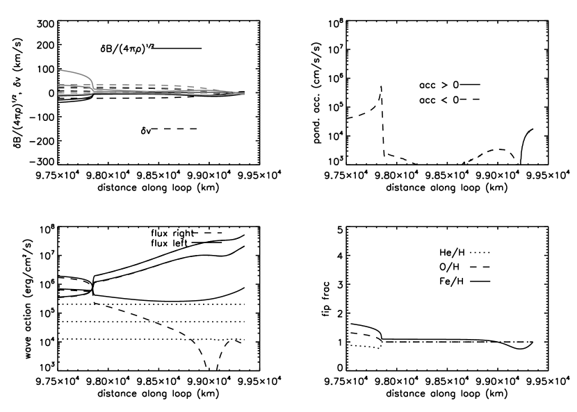
Figure 13: Same as figure 11 for the right hand side chromosphere “B”, where three Alfvén waves are launched up from the convection zone. The FIP fractions are reduced from those with a single incident wave, even though one of the waves here is on resonance. The contributions to the partial pressure of the other waves “dilute” the fractionation, by increasing the value of $v_{s}^{2}$ in the denominator of the integral in equation 6, without increasing the ponderomotive acceleration.

References

- Aellig et al. (2001) Aellig, M. R., Lazarus, A. J., & Steinberg, J. T. 2001, GRL, 28, 2767
- Antiochos (1994) Antiochos, S. K. 1994, Adv. Space Res., 14, 139
- Arge & Mullan (1998) Arge, C. N., & Mullan, D. J. 1998, Sol. Phys. 182, 293
- Asplund et al. (2004) Asplund, M., Grevesse, N., Sauval, A. J., Allende Prieto, C., & Kiselman, D. 2004, A&A, 417, 751
- Athay (1981) Athay, R. G. 1981, ApJ, 249, 340
- Athay (1994) Athay, R. G. 1994, ApJ, 423, 516
- Avrett & Loeser (2008) Avrett, E., & Loeser, R. 2008, ApJS, 175, 229
- Bahcall et al. (2005) Bahcall, J. N., Basu, S., & Serenelli, A. M. 2004, ApJ, 631, 1281
- Banaskiewicz et al. (1998) Banaskiewicz, M., Axford, W. I., & McKenzie, J. F. 1998, A&A, 337, 940
- Basu & Antia (2004) Basu, S., & Antia, H. M. 2004, ApJ, 606, L85
- Basu & Antia (2008) Basu, S., & Antia, H. M. 2008, Physics Reports, 457, 217
- Bogdan et al. (2003) Bogdan, T. J., et sl. 2003, ApJ, 599, 626
- Bryans et al. (2008) Bryans, P., Landi, E., & Savin, D. W. 2008, arXiv:0805.3302 [astro-ph]
- Caffau et al. (2008) Caffau, E., Ludwig, H.-G., Steffen, M., Ayres, T., Bonifacio, P., Cayrel, R., Freytag, B., & Plez, B. 2008, A&A, in press, arXiv:0805.4398 [astro-ph]
- Chae et al. (1998) Chae, J., Schühle, U., & Lemaire, P. 1998, ApJ, 505, 957
- Cranmer & van Ballegooijen (2005) Cranmer, S. R., & van Ballegooijen, A. A. 2005, ApJS, 156, 265
- Cranmer et al. (2007) Cranmer, S. R., van Ballegooijen, A. A., & Edgar, R. J. 2007, ApJS, 171, 520
- Dahlburg et al. (2005) Dahlburg, R. B.,Klimchuk, J. A., & Antiochos, S. K. 2005, ApJ, 622, 1191
- de Pontieu et al. (2007) De Pontieu, B., et al. 2007, Science, 318, 1574
- de Pontieu et al. (2005) De Pontieu, B., et al. 2005, ApJ, 624, L61
- Doschek, Dere, & Lund (1991) Doschek, G. A., Dere, K. P., & Lund, K. P. 1991, ApJ, 381, 583
- Drake & Testa (2005) Drake, J. J., & Testa, P. 2005, Nature, 436, 525
- Erdélyi & Fedun (2007) Erdélyi, R., & Fedun, V. 2007, Science, 318, 1572
- Feldman (1983) Feldman, U. 1983, ApJ, 275, 367
- Feldman (1987) Feldman, U. 1987, ApJ, 320, 426
- Feldman et al. (1998) Feldman, U., Schühle, U., Widing, K. G., & Laming, J. M. 1998, ApJ, 505, 999
- Feldman, Widing, & Lund (1990) Feldman, U., Widing, K. G., & Lund, P. A. 1990, ApJ, 364, L21
- Feldman & Laming (2000) Feldman, U., & Laming, J. M. 2000, Phys. Scripta., 61, 222
- Giammanco et al. (2008) Giammanco, C., Wurz, P., & Karrer, R. 2008, ApJ, 681, 1703
- Grevesse & Sauval (1998) Grevesse, N., & Sauval, A. J. 1998, Space Sci. Rev. 85, 161
- Henoux & Somov (1992) Henoux, J.-C., & Somov, B. V. 1992, Proceedings of the First SOHO WOrkshop, ESA SP-348, 325
- Henoux (1995) Henoux, J.-C. 1995, Adc. Space Res., 15, 23
- Henoux (1998) Henoux, J.-C. 1998, Space Science Reiews, 85, 215
- Hollweg (1984) Hollweg, J. V. 1984, ApJ, 277, 392
- Kasper et al. (2007) Kasper, J. C., Stevens, M. L., Lazarus, A. J., Steinberg, J. T., & Ogilive, K. W. 2007, ApJ, 660, 901
- Killie & Lie-Svendson (2007) Killie, M. A., & Lie-Svendson, Ø. 2007, ApJ, 666, 501
- Kingdon & Ferland (1996) Kingdon, J. B., & Ferland, G. J. 1996, ApJS, 106, 205
- Laming & Feldman (2001) Laming, J. M., & Feldman, U. 2001, ApJ, 546, 552
- Laming & Feldman (2003) Laming, J. M., & Feldman, U. 2003, ApJ, 591, 1257
- Laming (2004a) Laming, J. M. 2004a, ApJ, 614, 1063
- Laming (2004b) Laming, J. M. 2004b, ApJ, 604, 874
- Leroy & Schwartz (1982) Leroy, B., & Schwartz, S. J. 1982, A&A, 112, 84
- McDougall & Hood (2007) McDougal, A. M. D., & Hood, A. W. 2007, Solar Physics, 246, 259
- McIntosh et al. (2008) McIntosh, S. W., De Pontieu, B., & Tarbell, T. D. 2008, ApJ, 673, L219
- Muglach, Hofmann, & Staude (2005) Muglach, K., Hofmann, A., & Staude, J. 2005, A&A, 437, 1055
- Muglach (2003) Muglach,K. 2003, A&A, 401, 685
- Murphy & Share (2005) Murphy, R. J., & Share, G. H, 2005, Adv. Space Res. 35, 1825
- Parchevsky & Kosovichev (2007) Parchevsky, K. V., & Kosovichev, A. G. 2007, ApJ, 666, L53
- Peter (2001) Peter, H. 2001, A&A, 374, 1108
- Phillips et al. (1994) Phillips, K. J. H., Pike, C. D., Lang, J., Watanabe, T., & Takahashi, M. 1994, ApJ, 435, 888
- Schmelz et al. (2005) Schmelz, J. T., Nasraoui, K., Roames, J. K., Lippner, L. A., & Garst, J. W. 2005, ApJ, 634, L197
- Schwadron, Fisk, & Zurbuchen (1999) Schwadron, N. A., Fisk, L. A., & Zurbuchen, T. H. 1999, ApJ, 521, 859
- Schwartz & Leroy (1982) Schwartz, S. J., & Leroy, B. 1982, A&A, 112, 93
- Sheminova & Solanki (1999) Sheminova, V. A., & Solanki, S. K. 1999, A&A, 351, 701
- Terradas et al. (2008) Terradas, J., Arregui, I., Oliver, R., Ballester, J. L., Andries, J., & Goosens, M. 2008, ApJ, 679, 1611
- Tomczyk et al. (2007) Tomczyk, S., McIntosh, S. W., Keil, S. L., Judge, P. G., Schad, T., Seeley, D. H., & Edmondson, J. 2007, Science, 317, 1192
- van Doorsselaere et al. (2008) van Dooresselaere, T., Nakariakov, V. M., & Verwichte, E. 2008, ApJ, 676, L73
- Vernazza & Reeves (1978) Vernazza, J., & Reeves, E. M. 1978, ApJS, 37, 485
- Vernazza, Avrett, & Loeser (1981) Vernazza, J., Avrett, E. H., & Loeser, R. 1981, ApJS, 45, 635
- Vranjes et al. (2008) Vranjes, J., Poedts, S., Pandey, B. P., & De Pontieu, B. 2008, A&A, 478, 553
- Young (2005) Young, P. R. 2005, A&A, 444, L45
- Zaqarashvili & Roberts (2002) Zaqarashvili, T. V., & Roberts, B. 2002, PRE, 66, 026401
- Zaqarashvili & Roberts (2006) Zaqarashvili, T. V., & Roberts, B. 2006, A&A, 452, 1053
- Zurbuchen et al. (2002) Zurbuchen, T. H., Fisk, L. A., Gloeckler, G., & von Steiger, R. 2002, Geophys. Res. Lett. 29, 1352