Ruderman-Kittel-Kasuya-Yosida spin density oscillations: impact of the finite radius of the exchange interaction

Abstract

A non-interacting electron gas on a one-dimensional ring is considered at finite temperatures. The localized spin is embedded at some point on the ring and it is assumed that the interaction between this spin and the electrons is the exchange interaction being the basis of the Ruderman-Kittel-Kasuya-Yosida indirect exchange effect. When the number of electrons is large enough, it turns out that any small but finite interaction radius value can always produce an essential change of the spin density oscillations in comparison with the zero interaction radius traditionally used to model the Ruderman-Kittel-Kasuya-Yosida effect.

I Introduction

The Ruderman-Kittel-Kasuya-Yosida (RKKY) effect is a phenomenon which plays an important role in a formation of magnetic structures in different systems. The essence of the effect consists in an indirect interaction between localized spins placed in a Fermi sea of non-interacting conduction electrons. The interaction is called indirect because the spins feel the presence of each other through the electrons surrounding them: a localized spin interacting with the electrons induces in the electron gas spin density oscillations which then make impact on another localized spin. The interaction underlying the RKKY effect, that is the interaction between the localized spin and the electron gas, can be of different nature. It can be either the hyperfine interaction between a localized nuclear spin and conduction electrons Ruderman and Kittel (1954) or the exchange interaction between the conduction and localized electrons Kasuya (1956); Yosida (1957). The latter case is realized for example in alloys with transition metal ions where the conduction $s$-electrons and the localized $d$-electrons of an ion interact through the $s-d$ exchange interaction.

To model the RKKY effect it is traditionally assumed that the interaction between a localized spin and conduction electrons is local in the real space. This is modeled by Dirac’s delta function Kittel (1963); Harrison (1970). In the case of the hyperfine interaction this model looks quite plausible because the size of a nucleus, being of order $10^{-6}$ nm (see Ref. Krane, 1988), is small enough. The RKKY indirect exchange effect based on the hyperfine interaction was studied in the scientific literature. In Ref. Pershin et al., 2003 the RKKY interaction between nuclear spins embedded in a mesoscopic ring and a finite length quantum wire was investigated in the presence of a magnetic field. The indirect nuclear spin interaction was found to depend on the nuclear spin positions, number of the conduction electrons, magnetic field and system’s geometry. The influence of electron-electron interactions and electron spin correlations on the RKKY interaction between two nuclear spins was considered by Semiromi et al.Semiromi and Ebrahimi (2006) The nuclear spins were embedded in a mesoscopic metallic ring. It was numerically shown that the electron-electron interactions and electron spin correlations can essentially change the RKKY interaction dependence on the magnetic flux.

However, in the case of the exchange interaction the ionic spins are much less localized. For example, the ionic radius, which we will denote by $r_{0}$, for the $f$-shell metal ions Er³⁺ and Nd³⁺ is $r_{0}=0.096$ nm and $r_{0}=0.108$ nm (see Ref. Harrison, 1989), respectively. The value of $r_{0}$ gives an effective radius of the exchange interaction. Moreover, one can easily conceive a situation where artificial objects like quantum dots with non-zero total spin are embedded in a Fermi sea of conduction electrons. The interaction between the total spin of such objects and the electrons is similar to the exchange interaction and produces the RKKY interaction between the total spins of those artificial objects. The value of $r_{0}$ can thus be

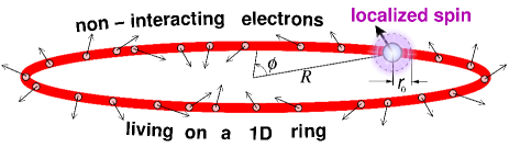
Figure 1: (Color online) A non-interacting electron gas on a 1D ring of radius $R$. The localized spin is centered around the ring point with the polar angle $\phi=0$. The localization radius of the spin is $r_{0}$ which is also estimated to be the radius of the exchange interaction in the RKKY effect.

technologically varied. Systems with quantum dots interacting through the RKKY effect were already investigated in a number of scientific papers. The RKKY effect between two quantum dots embedded in an Aharonov-Bohm ring was investigated by Utsumi et al.Utsumi et al. (2004) as a function of a magnetic flux through the ring. The quantum dots contained odd numbers of electrons. The interaction between the total quantum dots’ spins and the conduction electrons in the ring was described by a tunneling Hamiltonian. In this tunneling Hamiltonian the coupling constant was modeled by the delta function that is the interaction radius was $r_{0}=0$. In Ref. Rikitake and Imamura, 2005 two localized spins in one-, two- and three-dimensional electron gases were considered. Decoherence of the spins was studied using the kinetic equation for the reduced density matrix. Additionally, a quantum gate consisting of two quantum dots embedded in a two-dimensional electron gas of GaAs/AlGaAs heterostructure was investigated. The RKKY effect was provided through the $s-d$ exchange interaction which was assumed to take place just at the positions of the localized spins, that is the interaction radius was zero. Tamura et al.Tamura and Glazman (2005) studied the RKKY interaction between the localized spins of two quantum dots placed at the opposite edges of a one-dimensional (1D) conducting channel. The RKKY interaction between the spins across the channel was taken into account by virtue of an exchange interaction where the Fourier transform of the coupling constant was assumed to be momentum-dependent. This in principle means that the interaction could be non-local. However, consequences of this non-locality were out of focus of that work. In Ref. Aono, 2007 the RKKY interaction in a coupled quantum dot system embedded in a ring with a spin-orbit interaction was explored in the presence of the Aharonov-Bohm and Aharonov-Casher effects. The $s-d$ exchange interaction responsible for the RKKY effect in this system was also local.

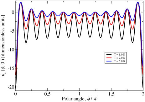
Figure 2: (Color online) The function $n_{\mathrm{s}}(\phi,r_{0})$ describing the spin density oscillations on a mesoscopic ring for the conventional model with $r_{0}=0$. The number of electrons is $N_{\mathrm{el}}=24$.

Finally, we would like to mention that effects of the finite size of the ionic spin distribution on the RKKY interaction have been studied in bulk systems in connection with ferromagnetic Heusler alloys Darby (1977a); Smit (1977); Darby (1977b); Malmström and Geldart (1978); Smit (1978). However, the models used in those attempts did not give the delta function in the limit $r_{0}\rightarrow 0$.

The purpose of the present work is to verify by means of a simple model whether in a mesoscopic ring a finite value of $r_{0}$ can play any role in the formation of the electron spin density oscillations which underpin the RKKY indirect exchange interaction. In the limit $r_{0}\rightarrow 0$ the model which we use gives the delta function. It is shown that if the interaction radius is finite, its impact on the electron spin density oscillations is to reduce the oscillation amplitude. An interesting feature is that when the number of the electrons in the gas is large enough, this reduction, produced by the presence of a small domain of size $r_{0}$, is significant and takes place in the whole system with much larger size.

The paper is organized as follows. Sec. II describes a mathematical formulation of the problem. In Sec. III the solution is obtained using the Matsubara diagrammatic approach. The results are discussed in Sec. IV.

II Theoretical model

We consider a non-interacting Fermi-gas on a 1D ring of radius $R$. The electron positions are specified by the polar angle $\phi$. An ion (or another object) with a non-zero total spin is placed on the ring at $\phi=0$. The system is schematically shown in Fig. 1. The interaction between the localized spin and conduction electrons is assumed to be an exchange interaction which in general can be non-local.

To formulate the problem mathematically we write down the Hamiltonian of the system in the form:

$$\hat{H}=\hat{H}_{0}+\hat{H}_{\mathrm{int}}.$$ (1)

In Eq. (1) $\hat{H}_{0}$ is the Hamiltonian of the non-interacting $N$-electron system on a 1D ring:

$$\hat{H}_{0}=\sum_{i=1}^{N}\hat{H}_{0}^{i},$$ (2)

with

$$\hat{H}_{0}^{i}=-\frac{\hbar^{2}}{2mR^{2}}\frac{\partial^{2}}{\partial\phi_{i}^{2}}$$ (3)

where $m$ is the electron mass and $\phi_{i}$ is the $i$-th electron coordinate. The spin-degenerate eigen-values of the single-particle Hamiltonian $\hat{H}_{0}^{i}$ are

$$\epsilon_{n\sigma}=\frac{\hbar^{2}n^{2}}{2mR^{2}},$$ (4)

where $n=0,\pm 1,\ldots$ and $\sigma$ is the spin index. The normalized eigen-states of $\hat{H}_{0}^{i}$, $|n\sigma\rangle$, in the coordinate representation are

$$\langle\phi\sigma^{\prime}|n\sigma\rangle=\delta_{\sigma\sigma^{\prime}}\frac{1}{\sqrt{2\pi}}\exp(-in\phi).$$ (5)

The term $\hat{H}_{\mathrm{int}}$ in Eq. (1) describes the exchange interaction between the localized spin and the electron gas and it is conventionally written as:

$$\hat{H}_{\mathrm{int}}=\sum_{j=1}^{N}J(\phi_{j})S^{i}\sigma_{j}^{i},$$ (6)

where $J(\phi)$ is the coupling function of the exchange interaction, ${\bf S}$ is the localized spin placed at $\phi=0$, ${\bf\sigma}_{j}$ is the vector of the electron spin Pauli matrices and the summation over the index $i$ is assumed.

As it was mentioned above, traditionally it is assumed that the exchange interaction is local, that is the embedded spin interacts with the electrons only at $\phi=0$. In this case the coupling function $J(\phi)$ is modeled by the following dependence on the polar angle:

$$J(\phi)=J\delta(\phi),$$ (7)

where $J$ is a coupling constant.

In this work we suggest a simple model in which the localized spin interacts with the electrons in a small vicinity of the point $\phi=0$ and when the vicinity is tightened into a point at $\phi=0$, the model turns into the conventional one (7):

$$J(\phi)=\frac{J}{\phi_{0}\sqrt{\pi}}\begin{cases}\exp\bigl{[}-\bigl{(}\frac{\phi}{\phi_{0}}\bigl{)}^{2}\bigl{]},&0\leqslant\phi<\pi,\\ \exp\bigl{[}-\bigl{(}\frac{2\pi-\phi}{\phi_{0}}\bigl{)}^{2}\bigl{]},&\pi\leqslant\phi<2\pi.\end{cases}$$ (8)

The size $\phi_{0}=r_{0}/R$ of this vicinity is estimated from the radius $r_{0}$ of the ion (or from a characteristic size of another object) which is the source of the spin centered around $\phi=0$. Using the well known representation of Dirac’s delta function,

$$\delta(x)=\underset{t\rightarrow 0}{\mathrm{lim}}\frac{\exp\bigl{[}-\bigl{(}\frac{x}{\sqrt{t}}\bigl{)}^{2}\bigl{]}}{\sqrt{\pi t}},$$ (9)

one is convinced that the non-local model, Eq. (8), takes the local form, Eq. (7), when $r_{0}\rightarrow 0$.

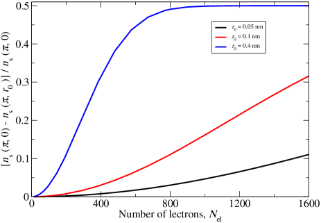
Figure 3: (Color online) The relative change of the spin density at $\phi=\pi$ (the furthermost point from the localized spin). The reference is the spin density at $r_{0}=0$. The temperature is $T=1K$.

To study whether finite values of $r_{0}$ have any effect we will calculate the electron spin density at finite temperatures. The electron spin density operator at point $\phi$ on the ring is defined as

$$\hat{n}_{\mathrm{s}}^{i}(\phi)=\sum_{j=1}^{N}\delta(\phi_{j}-\phi)\sigma_{j}^{i}.$$ (10)

The electron spin density at point $\phi$ is obtained through the statistical average using the Gibbs grand canonical ensemble:

$$n_{\mathrm{s}}^{i}(\phi,r_{0})=\frac{\mathrm{Tr}\bigl{[}\exp\bigl{(}-\frac{\hat{H}-\mu\hat{N}}{k_{\mathrm{B}}T}\bigl{)}\hat{n}_{s}^{i}(\phi)\bigl{]}}{Z},$$ (11)

where we explicitly show that the electron spin density is also a function of the interaction radius $r_{0}$. In Eq. (11) $Z$ is the partition function:

$$Z=\mathrm{Tr}\biggl{[}\exp\biggl{(}-\frac{\hat{H}-\mu\hat{N}}{k_{\mathrm{B}}T}\biggl{)}\biggl{]}.$$ (12)

In Eqs. (11) and (12) $k_{\mathrm{B}}$ is the Boltzmann constant, $\mu$ is the chemical potential, $T$ is the temperature, $\hat{N}$ is the particle number operator and the trace is taken using a complete set of states of the Fock space. It is also important to note that since the number $N$ of electrons is fixed, the chemical potential $\mu$ is not an independent variable but a function of the temperature $T$.

III Imaginary time Green’s function solution

The problem formulated in the previous section is obviously not solvable exactly. Thus some approximation methods should be applied. For small values of the coupling constant $J$ in Eq. (8) a perturbation theory, where $\hat{H}_{\mathrm{int}}$ is considered as a perturbation, can be applied. As the calculations are performed at finite temperatures, instead of the pure quantum mechanical perturbation theory one has to use the so-called thermodynamic perturbation theory Landau and Lifshitz (1980) for the quantum statistical averages. This perturbation theory is in general valid when the perturbation energy per particle is less than $k_{\mathrm{B}}T$, i.e., $J<k_{\mathrm{B}}T$. However, very often it happens that when $T\rightarrow 0$, the coefficients of the perturbation expansion change as functions of $T$ in such a way that the thermodynamic perturbation theory can remain valid for all temperatures.

Although the thermodynamic perturbation theory gives a general approach to calculate statistical averages, in its original form it is quite cumbersome. It is more convenient to use this theory reformulated in terms of a diagrammatic approach, namely the Matsubara (or imaginary time) diagrammatic method Abrikosov et al. (1963).

In order to employ this technique for our purposes we first rewrite the total Hamiltonian of the problem, Eq. (1), in the second quantized form using the $\{n\sigma\}$ single-particle basis:

$$\begin{split}&\hat{H}=\sum_{n\sigma}\epsilon_{n\sigma}a^{\dagger}_{n\sigma}a_{n\sigma}+\frac{JS^{i}}{2\pi}\sum_{n\sigma\,n^{\prime}\sigma^{\prime}}\langle\sigma|\hat{\sigma}^{i}|\sigma^{\prime}\rangle\times\\ &\times\biggl{\{}\frac{1}{\phi_{0}\sqrt{\pi}}\int_{\pi}^{\pi}\,d\tilde{\phi}\exp\biggl{[}-\biggl{(}\frac{\tilde{\phi}}{\phi_{0}}\biggl{)}^{2}\biggl{]}\times\\ &\times\exp[i\tilde{\phi}(n-n^{\prime})]\biggl{\}}a^{\dagger}_{n\sigma}a_{n^{\prime}\sigma^{\prime}}.\end{split}$$ (13)

The second quantized form of the electron spin density operator at point $\phi$ is

$$\hat{n}_{\mathrm{s}}^{i}(\phi)=\frac{1}{2\pi}\sum_{n\sigma\,n^{\prime}\sigma^{\prime}}\langle\sigma|\hat{\sigma}^{i}|\sigma^{\prime}\rangle\exp[i\phi(n-n^{\prime})]a^{\dagger}_{n\sigma}a_{n^{\prime}\sigma^{\prime}}$$ (14)

and the expression for the electron spin density at point $\phi$ may be rewritten as

$$n_{\mathrm{s}}^{i}(\phi,r_{0})=-\sum_{\sigma\sigma^{\prime}}\langle\sigma^{\prime}|\hat{\sigma}^{i}|\sigma\rangle\mathcal{G}_{\sigma\sigma^{\prime}}(\phi,\tau;\phi,\tau).$$ (15)

In the last expression $\mathcal{G}_{\sigma\sigma^{\prime}}(\phi,\tau;\phi^{\prime},\tau^{\prime})$ is the one-particle imaginary time Green’s function defined as

$$\begin{split}&\mathcal{G}_{\sigma\sigma^{\prime}}(\phi,\tau;\phi^{\prime},\tau^{\prime})=\\ &=\frac{1}{Z}\mathrm{Tr}\biggl{[}\exp\biggl{(}-\frac{\hat{H}-\mu\hat{N}}{k_{\mathrm{B}}T}\biggl{)}\mathrm{T}\hat{\psi}_{\sigma}(\phi,\tau)\hat{\psi}_{\sigma^{\prime}}^{\dagger}(\phi^{\prime},\tau^{\prime})\biggl{]},\end{split}$$ (16)

where $\mathrm{T}$ is the time-ordering operator and $\hat{\psi}_{\sigma}(\phi,\tau)$ are the imaginary time field operators,

$$\begin{split}&\hat{\psi}_{\sigma}(\phi,\tau)=\\ &=\exp[\tau(\hat{H}-\mu\hat{N})]\hat{\psi}_{\sigma}(\phi)\exp[-\tau(\hat{H}-\mu\hat{N})],\end{split}$$ (17)

with $\hat{\psi}_{\sigma}(\phi)$ related to the annihilation operators $a_{n\sigma}$ as

$$\hat{\psi}_{\sigma}(\phi)=\frac{1}{\sqrt{2\pi}}\sum_{n}\exp(-i\phi n)a_{n\sigma}.$$ (18)

We now apply the diagrammatic expansion of the Green’s function $\mathcal{G}_{\sigma\sigma^{\prime}}(\phi,\tau;\phi^{\prime},\tau^{\prime})$. The effect of the RKKY spin density oscillations appears already in the first order and thus we only need to consider the first order diagram. Such an approach to the RKKY spin density oscillations was considered in Ref. Levitov and Shitov, 2003 for a three-dimensional electron gas. However, in that case the electron spectrum was continuous and to perform momentum integrals the linearization of the spectrum on the Fermi-surface was employed to get the long range behavior of the RKKY oscillations. In our problem the electron spectrum is discrete and instead of integrals we will have sums over discrete indices. Moreover, since our system is finite we are interested in the RKKY oscillations in the whole range and not only at long distances from the localized spin.

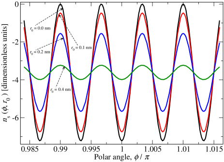
Figure 4: (Color online) The electron spin density oscillations in the vicinity of the point $\phi=\pi$. The number of electrons is $N_{\mathrm{el}}=600$. The temperature is $T=1K$.

The first order contribution to the Green’s function $\mathcal{G}_{\sigma\sigma^{\prime}}(\phi,\tau;\phi^{\prime},\tau)$ is

$$\begin{split}&\mathcal{G}_{\sigma\sigma^{\prime}}^{(1)}(\phi,\tau;\phi^{\prime},\tau)=-\frac{JS^{i}}{(2\pi)^{2}\hbar}\langle\sigma|\hat{\sigma}^{i}|\sigma^{\prime}\rangle\times\\ &\times\sum_{n\,n^{\prime}}\exp(-in\phi+in^{\prime}\phi^{\prime})j_{n\,n^{\prime}}s_{n\,n^{\prime}},\end{split}$$ (19)

where

$$\begin{split}&j_{n\,n^{\prime}}=\exp\biggl{[}-\frac{1}{4}(n-n^{\prime})^{2}\phi_{0}^{2}\biggl{]}\times\\ &\times\mathrm{Re}\biggl{\{}\mathrm{erf}\biggl{[}\frac{\pi}{\phi_{0}}+\frac{i}{2}(n-n^{\prime})\phi_{0}\biggl{]}\biggl{\}},\end{split}$$ (20)

and

$$s_{n\,n^{\prime}}=\begin{cases}\hbar\frac{n_{n^{\prime}}-n_{n}}{\epsilon_{n^{\prime}}-\epsilon_{n}},&n^{\prime 2}\neq n^{2},\\ -n_{n}(1-n_{n})\frac{\hbar}{k_{\mathrm{B}}T},&n^{\prime 2}=n^{2}\end{cases}$$ (21)

with $n_{n}$ being the fermion occupation numbers,

$$n_{n}=\frac{1}{\exp(\frac{\epsilon_{n}-\mu}{k_{\mathrm{B}}T})+1}.$$ (22)

Since $\phi_{0}\ll\pi$, we have

$$j_{n\,n^{\prime}}\approx\exp\biggl{[}-\frac{1}{4}(n-n^{\prime})^{2}\phi_{0}^{2}\biggl{]}$$ (23)

and this approximation will be used in the calculations below.

Substituting Eq. (19) into Eq. (15) and taking into account Eq. (21), we obtain the first order contribution to the electron spin density

$$n_{\mathrm{s}}^{i}(\phi,r_{0})=\frac{2JS^{i}}{(2\pi)^{2}}n_{\mathrm{s}}(\phi,r_{0}),$$ (24)

where $n_{\mathrm{s}}(\phi,r_{0})$ is given by the following expression:

$$\begin{split}&n_{\mathrm{s}}(\phi,r_{0})=\!\!\!\!\!\sum_{\begin{subarray}{c}n\,n^{\prime}\\ (n^{\prime 2}\neq n^{2})\end{subarray}}\exp[-i(n-n^{\prime})\phi]j_{n\,n^{\prime}}\frac{n_{n^{\prime}}-n_{n}}{\epsilon_{n^{\prime}}-\epsilon_{n}}-\\ &-\sum_{\begin{subarray}{c}n\,n^{\prime}\\ (n^{\prime 2}=n^{2})\end{subarray}}\exp[-i(n-n^{\prime})\phi]j_{n\,n^{\prime}}\frac{n_{n}(1-n_{n})}{k_{\mathrm{B}}T}.\end{split}$$ (25)

For a given value of the interaction radius $r_{0}$ the function $n_{\mathrm{s}}(\phi,r_{0})$ provides an oscillatory behavior of the electron spin density as a function of the polar angle $\phi$.

IV Results and discussion

In this section we numerically analyze the electron spin density oscillations. Using Eq. (25) we calculate the function $n_{\mathrm{s}}(\phi,r_{0})$. The mesoscopic ring is assumed to be fabricated on AlGaAs-GaAs heterostructures. The values of the parameters are taken close to the ones used in previous works Utsumi et al. (2004) and in experiments Fuhrer et al. (2001). The ring radius is $R=40$ nm, the effective mass $m=0.067m_{0}$, where $m_{0}$ is the free electron mass.

Let us first consider the behavior of $n_{\mathrm{s}}(\phi,r_{0})$ as a function of the polar angle for the conventional model with $r_{0}=0$. It is shown in Fig. 2 for different values of the temperature $T$ and for the number of electrons $N_{\mathrm{el}}=24$. In systems with a continuous spectrum the RKKY spin density oscillations behave like $\cos(2p_{\mathrm{F}}r/\hbar)$ (similar to the Friedel oscillations of the electronic density) where $p_{\mathrm{F}}$ is the Fermi momentum and $r$ is the distance from the localized spin. In our case the spectrum is discrete. The analog of the Fermi momentum is the energy level number $n_{\mathrm{F}}$ such that at $T=0$ the states with $|n|>n_{\mathrm{F}}$ are not populated. Since the state with a given value of $n$ can be occupied by two electrons, for $N_{\mathrm{el}}=24$ one gets $n_{\mathrm{F}}=6$ and thus $2n_{\mathrm{F}}=12$. In agreement with this estimation Fig. 2 shows 12 oscillations. As it was discussed in the literature (see, for example, Ref. Levitov and Shitov, 2003), the effect of the temperature on the RKKY spin density oscillations is to produce a faster reduction of the oscillation amplitude with the distance from the localized spin. For example in three-dimensional electron gases at $T=0$ the oscillation amplitude at large distances decreases as $1/r^{3}$ and at finite temperatures it is damped at the thermal distance $\hbar p_{\mathrm{F}}/(2\pi mk_{\mathrm{B}}T)$. An analogous behavior takes place in our case as well. As it can be seen from Fig. 2 the amplitude of the oscillations as a function of the polar angle is damped faster for higher values of the temperature.

Next we turn our attention to the effect of the finite interaction radius $r_{0}$ of the exchange interaction on the electron spin density oscillations. From Eq. (23) it seems that for realistic, that is small, values of $\phi_{0}$ the function $j_{n\,n^{\prime}}\approx 1$ and a finite interaction radius value does not produce any change in the electron spin density oscillations in comparison with the case $r_{0}=0$. However, this reasoning is not entirely correct because it does not take into consideration the number of electrons in the gas surrounding the localized spin in the ring. Indeed, when the number of electrons in the gas grows, energy levels with higher values of $|n|$ become important. The contributions with higher values of $|n-n^{\prime}|$ are involved. From Eqs. (23) and (25) one observes that in parallel with this involvement the contributions from terms with high values of $|n-n^{\prime}|$ get more suppressed. It does not matter how small the interaction radius is. The main point is that it is finite. For any finite value of $r_{0}$ there exists a number of electrons $N_{\mathrm{c}}$ in the gas such that for $N_{\mathrm{el}}>N_{\mathrm{c}}$ the interaction radius, no matter how small it is, will produce more and more pronounced impact on the spin density. This is demonstrated in Fig. 3 where the relative change of the spin density at $\phi=\pi$ is depicted as a function of the number of the electrons in the gas for different values of the interaction radius $r_{0}$. As expected the change of the electron spin density in comparison with the conventional model with $r_{0}=0$ is negligible for small numbers of the electron in the ring. For larger numbers of the electrons the electron spin density for finite values of $r_{0}$ starts to deviate from the model with $r_{0}=0$. It is interesting that even the interaction radius $r_{0}=0.05$ nm can produce an observable change of approximately 11% for $N_{\mathrm{el}}=1600$. The ring distance between the two points $\phi=0$ and $\phi=\pi$ is about 126 nm while the size of the area where the spin is localized is 0.1 nm, that is three orders of magnitude less. An important result is that the small vicinity around the localized spin is able to significantly change the electron spin density in every point of the system whose size is several orders of magnitude larger than the size of the domain over which the localized spin is spread.

The RKKY spin density oscillations for $N_{\mathrm{el}}=600$ are displayed in Fig. 4 for different values of $r_{0}$. In this case the number of the oscillations is approximately equal to 300 and thus only a small vicinity around $\phi=\pi$ is plotted to clearly show the oscillations.

Finally, we note that semi-quantitatively the oscillating behavior can be explained by the dominance of the term $\cos(2n_{\mathrm{F}}\phi)j_{n_{\mathrm{F}},-n_{\mathrm{F}}}n_{n_{\mathrm{F}}}(1-n_{n_{\mathrm{F}}})$ in Eq. (25). The $2n_{\mathrm{F}}$ RKKY oscillations with $r_{0}=0$ are weighted with $j_{n_{\mathrm{F}},-n_{\mathrm{F}}}<1$. For small $N_{\mathrm{el}}$ the weight $j_{n_{\mathrm{F}},-n_{\mathrm{F}}}\approx 1$ and plays no role but for large $N_{\mathrm{el}}$ this weight reduces the amplitude of the $2n_{\mathrm{F}}$ RKKY oscillations by the factor $\exp[-(n_{\mathrm{F}}\phi_{0})^{2}]$.

V Summary

The Ruderman-Kittel-Kasuya-Yosida (RKKY) spin density oscillations, induced by an exchange interaction between a localized spin and the electron gas in which the spin is embedded, have been investigated at finite temperatures taking into account finite values of the exchange interaction radius. It has been found that the electron spin density in a non-interacting gas on a mesoscopic ring is changed in comparison with the traditional model which assumes that the interaction radius is zero. The amplitude of the RKKY oscillations is suppressed when the number of the electrons in the gas increases. This suppression gets stronger for larger values of the interaction radius.

A remarkable point is that as soon as the interaction radius is finite, it is already not important how small it is because its impact always becomes observable when the number of the electrons in the ring is large enough.