Unsupervised bayesian convex deconvolution based on a field with an explicit partition function

Abstract

This paper proposes a non-Gaussian Markov field with a special feature: an explicit partition function. To the best of our knowledge, this is an original contribution. Moreover, the explicit expression of the partition function enables the development of an unsupervised edge-preserving convex deconvolution method. The method is fully Bayesian, and produces an estimate in the sense of the posterior mean, numerically calculated by means of a Monte-Carlo Markov Chain technique. The approach is particularly effective and the computational practicability of the method is shown on a simple simulated example.

I Introduction

The research concerning regularization for ill-posed inverse problems was first carried out by Phillips, Twomey and Tikhonov  in the sixties and are compiled in [1]. For the specific problem of deconvolution they lead to the contributions of Hunt [2] based on toroidal models and fast implementation by fft. These methods rely on quadratic penalization i.e., Gaussian laws in a Bayesian framework. The solutions thus formulated are linear w.r.t. the data and numerically efficient. However, their resolution is limited: the capability to properly restore sharp edges is limited.

At the beginning of the eighties, in order to overcome these limitations, Geman & Geman [3] (see also [4]) introduced a much superior Markovian field including hidden variables [5]. The hidden variables (also referred to as dual or auxiliary variable) are binary and interactive variables modeling sharp edges and closed contours. The data processing then relies on a detection-estimation strategy and allows the recovery of distinct zones with abrupt changes. The calculation of the solution in the sense of the maximum a posteriori is based on a simulated annealing algorithm which requires intensive numerical computations. For the sake of computational efficiency in some cases, Geman & Reynolds [6] and then Geman & Yang [7] introduced auxiliary (also referred to as dual) variables: the sampling of a correlated non-Gaussian field reduces to the sampling of a correlated Gaussian field for one part and to the sampling of a separable field for the other. Furthermore, the construction proposed by [7] is founded on the work of Hunt and the toroidal models: the sampling of the correlated Gaussian field reduces to the sampling of an inhomogeneous white Gaussian field followed by an fft. The proposal below takes advantage of this construction.

The case of fields with convex potential [8, 9, 10, 11, 12, 13] (see also [14, 15]) was laid down in the nineties as fulfilling a compromise between the quality of the reconstructed images and the computational burden. In this framework, a particular attention has been paid to the case of $\mbox{L}_{2}-\mbox{L}_{1}$ potentials [9, 10, 11, 12, 13]: a quadratic behavior around the origin and a linear behavior at large values allow edge preservation. In this context, the constructions of [6] and [7] respectively led to two algorithms: ARTHUR and LEGEND [16] (see also [17]). The work presented here concerns this type of potential.

With such potentials, the regularized solutions usually necessitate the adjustment of three hyperparameters: two parameters to control the law for the image and one parameter to control the law for the noise. Several attempts are dedicated to the question of hyperparameter estimation and the investigated solutions are frequently based on statistical approaches: (approximated or pseudo) likelihood, Bayesian strategies, EM and SEM algorithms…The reader may consult papers such as [18, 19, 20, 21, 22, 23, 24] and reference books such as [25, Part.VI], [26, Ch.7] or [27, Ch.8]. These approaches are potentially very powerful but they come up against a major difficulty: the partition function of existing a priori fields depends on hyperparameters and is not explicitly given.

The first novelty of the paper lies in the fact that it proposes a new random field with an explicit partition function. To this end, the paper build an original type of compound (toroidal) field with $\mbox{L}_{2}-\mbox{L}_{1}$ potential. The work is largely inspired by the Bayesian interpretation of dual variables in terms of Location Mixture of Gaussian proposed by [28]. Moreover, it is also inspired by [29] (itself based on the contributions of Hunt [2] and Geman & Yang [7]). However, none of these contributions put forward the idea of a field with an explicit partition function. Afterwards, the paper proposes a second novelty: a full Bayesian unsupervised (i.e., including hyperparameter estimation) edge-preserving convex deconvolution method, thanks to the knowledge of the partition function. It is based on a posterior law for the whole set of unknown parameters (including hyperparameters) and a Minimum Mean Square Error strategy.

The paper is presented in the following manner. Section II introduces the notations and states the problem. Section III is devoted to the construction of the proposed field, Section IV proposes its use for image deconvolution and demonstrates the numerical practicability. Conclusions and perspectives are delivered in Section V. Most of the calculations are explained in Appendices A to H.

II Notation and problem statement

Work is carried out on $P\times P$ real images, with $N=P^{2}$ pixels, represented in a matrix form. $a_{pq}$ denotes the generic element of the matrix ${\mathb{A}}$, $N_{2}({\mathb{A}})=\sum|\,a_{pq}\,|^{2}$ its squared norm and $\overset{\kern-3.30002pt~{}_{\circ}}{{\mathb{A}}}$ its fft-2d. The transformation is normalized: the Parseval relationship is written as $N_{2}({\mathb{A}})=N_{2}(\overset{\kern-3.30002pt~{}_{\circ}}{{\mathb{A}}})$ and the sum of the pixels is $\sum a_{pq}=P\,\overset{\kern-3.30002pt~{}_{\circ}}{a}_{\scriptscriptstyle 00}$. The symbols $\star$ and $\otimes$ respectively represent the circular convolution and the Schur product (termwise) of matrices. If ${\mathb{F}}$ represents a circular filter and ${\mathb{I}}$ an input object, the output is written ${\mathb{O}}={\mathb{F}}\star{\mathb{I}}$ in the spatial domain resulting in $\overset{\kern-3.30002pt~{}_{\circ}}{{\mathb{O}}}=\overset{\kern-3.30002pt~{}_{\circ}}{{\mathb{F}}}\otimes\overset{\kern-3.30002pt~{}_{\circ}}{{\mathb{I}}}$ in the Fourier domain. If $\overset{\kern-3.30002pt~{}_{\circ}}{f}_{pq}\neq 0$ for all $p,q$, the associated filter is invertible.

In the subsequent developments about deconvolution, ${\mathb{Y}}$, ${\mathb{X}}$, ${\mathb{H}}$, and ${\mathb{N}}$ respectively denote the observed data, the unknown object, the convolution matrix and the observation noise. With these notations, the observation equation is written:

$${\mathb{Y}}={\mathb{H}}\star{\mathb{X}}+{\mathb{N}}\,.$$ (1)

The deconvolution problem consists in recovering the unknown object ${\mathb{X}}$ given the observed data ${\mathb{Y}}$ and given the observation model ${\mathb{H}}$. The ill-posedness of the problem has been well identified for several decades and the problem is nowadays often tackled in a Bayesian framework using Markov priors. In a Gibbs form, the prior law writes:

$$f_{{\mathcal{X}}}\left[{\mathb{X}}\right]=K_{{\mathcal{X}}}^{-1}~{}\exp\left[-\Phi_{\boldsymbol{\theta}}\left({\mathb{X}}\right)\right]\,,$$

where $K_{{\mathcal{X}}}$ is the partition function (normalizing constant) and $\Phi_{\boldsymbol{\theta}}$ is the Gibbs energy controlled by a set of parameters (such as variance, threshold, scale, correlation length…) collected in a vector ${\boldsymbol{\theta}}$. The general methodology is well-known: the solution is determined from the a posteriori law and a point estimate can be chosen as the mean or the maximizer, for instance. Anyway, the posterior law (and the point estimates) depends upon hyperparameters notably on the parameters of the prior ${\boldsymbol{\theta}}$. The inference about these parameters can be attempted in a statistical framework whose keystone is an exact and explicit likelihood function (in an usual sense or in a posterior sense). This function is itself founded on a complete expression for the prior law including the partition function as it depends on ${\boldsymbol{\theta}}$. It is given as a large dimension integral:

$$K_{{\mathcal{X}}}=K_{{\mathcal{X}}}({\boldsymbol{\theta}})=\displaystyle\int_{{\mathbbm{R}}^{N}}\exp\left[\,-\Phi_{\boldsymbol{\theta}}\left({\mathb{X}}\right)\,\right]~{}{\mathrm{d}}{\mathb{X}}\,.$$ (2)

It is a commonplace to say that $K_{{\mathcal{X}}}({\boldsymbol{\theta}})$ can be explicitly given for two well-known classes of (continuous state) field:

• $\Phi$ is quadratic, i.e., the field is Gaussian

• $\Phi$ is separable, i.e., the field is white.

In other cases and especially for non-separable and non-Gaussian fields, the theoretical calculation and the numerical computation of (2) are desperate tasks [25, p.281] and they have never been achieved. However, its achievement is made possible and simple in the next Section, for a special non-separable and non-Gaussian field.

III Prior Field with Partition Function

Taking advantage of ($i$) and ($ii$) above, the proposed random field is a compound field involving two variables: a pixel variable noted as ${\mathcal{X}}$ and an auxiliary (or dual or hidden) variable noted as ${\mathcal{B}}$. The joint law for $({\mathcal{X}},{\mathcal{B}})$ is defined by the law of ${\mathcal{X}}|{\mathcal{B}}$ for one part and by the law of ${\mathcal{B}}$ for the other part. The former is a Gaussian component (case ($i$) above) and the latter is a separable component (case ($ii$) above).

III-A Toroidal Gaussian Field for ${\mathcal{X}}|{\mathcal{B}}$

Let us consider two matrices ${\mathb{B}}$ and ${\mathb{F}}$ with $\overset{\kern-3.30002pt~{}_{\circ}}{f}_{pq}\neq 0$ for all $p,q$ and the toroidal (circular shift invariant) Gaussian field with a density parametrized in the form:

$$f_{{\mathcal{X}}|{\mathcal{B}}}\left[{\mathb{X}}|{\mathb{B}}\right]=K_{{\mathcal{X}}|{\mathcal{B}}}^{-1}~{}\exp\left[-\gamma_{\mathrm{d}}\,N_{2}({\mathb{F}}\star{\mathb{X}}-{\mathb{B}})/2\right]\,,$$ (3)

where $\gamma_{\mathrm{d}}>0$ is an inverse variance. The matrix ${\mathb{F}}$ designs the field structure and especially the neighborhood system and the form of the cliques. In the Fourier domain, the potential is separable and naturally develops in two forms:

$$N_{2}({\mathb{F}}\star{\mathb{X}}-{\mathb{B}}) = N_{2}\left(\overset{\kern-3.30002pt~{}_{\circ}}{{\mathb{F}}}\otimes\overset{\kern-3.30002pt~{}_{\circ}}{{\mathb{X}}}-\overset{\kern-3.30002pt~{}_{\circ}}{{\mathb{B}}}\right)$$

$$= \sum_{pq}|\,\overset{\kern-3.30002pt~{}_{\circ}}{f}_{pq}\,\overset{\kern-3.30002pt~{}_{\circ}}{x}_{pq}-\overset{\kern-3.30002pt~{}_{\circ}}{b}_{pq}\,|^{2}$$

$$= \sum_{pq}|\,\overset{\kern-3.30002pt~{}_{\circ}}{f}_{pq}|^{2}~{}|\,\overset{\kern-3.30002pt~{}_{\circ}}{x}_{pq}-\overset{\kern-3.30002pt~{}_{\circ}}{b}_{pq}/\overset{\kern-3.30002pt~{}_{\circ}}{f}_{pq}\,|^{2}$$

which has three essential consequences for the following developments.

1. The law for $\overset{\kern-3.30002pt~{}_{\circ}}{{\mathcal{X}}}$ is separable and each $\overset{\kern-3.30002pt~{}_{\circ}}{X}_{pq}$ is Gaussian with mean $\overset{\kern-3.30002pt~{}_{\circ}}{b}_{pq}/\overset{\kern-3.30002pt~{}_{\circ}}{f}_{pq}$ and inverse variance $\gamma_{\mathrm{d}}|\overset{\kern-3.30002pt~{}_{\circ}}{f}_{pq}|^{2}$. As a result, the sampling of ${\mathcal{X}}$ reduces to the sampling of an inhomogeneous white Gaussian noise followed by an fft-2d.

2. The change of variable $\overline{{\mathcal{X}}}={\mathb{F}}\star{\mathcal{X}}$ is invertible, $\overline{{\mathcal{X}}}$ is white and each $\overline{X}_{pq}$ is Gaussian with mean $b_{pq}$ and common inverse variance $\gamma_{\mathrm{d}}$.

3. The partition function $K_{{\mathcal{X}}|{\mathcal{B}}}$ is easily tractable in the Fourier domain thanks to a change of variable

   $$K_{{\mathcal{X}}|{\mathcal{B}}} = \displaystyle\int_{{\mathbbm{R}}^{N}}\exp\left[-\gamma_{\mathrm{d}}\,N_{2}({\mathb{F}}\star{\mathb{X}}-{\mathb{B}})/2\right]~{}{\mathrm{d}}{\mathb{X}}$$

   $$= \left[\gamma_{\mathrm{d}}^{\,N/2}~{}~{}\left(2\pi\right)^{-N/2}~{}\prod|\overset{\kern-3.30002pt~{}_{\circ}}{f}_{pq}|\right]^{-1}\,,$$

   and does not depend on ${\mathb{B}}$.

In relation to existing works such as [7, 16, 27, 29, 28], the main idea here is simply to focus on the case where the change of variable $\overline{{\mathcal{X}}}={\mathb{F}}\star{\mathcal{X}}$ is invertible (point 2 above) that is to say the number of cliques and the number of pixels are equal.

Remark 1

—  The partition function $K_{{\mathcal{X}}|{\mathcal{B}}}$ does not depend on ${\mathb{B}}$ as a counterpart of a limitation: the number of cliques and the number of pixels are equal. As an illustration of the limitation, let us point out that $K_{{\mathcal{X}}|{\mathcal{B}}}$ depends on ${\mathb{B}}$ for a field based on horizontal cliques plus vertical cliques (the number of cliques is greater than the number of pixels).

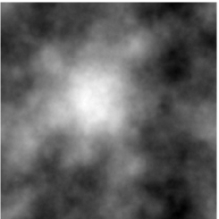
Figure 1: A sample of the field, with $\gamma_{\mathrm{d}}=\gamma_{\mathrm{b}}=1$ ($\varepsilon$ is also set to 1).

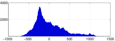
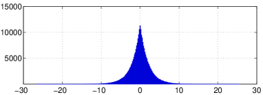
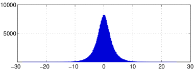
Figure 2: Histograms (image at Fig. 1). From top to bottom: histogram of image pixels $X$, histogram of auxiliary variables $B$ and histogram of differences $\overline{X}$.

III-B Compound Field

A separable and homogeneous field is then introduced for the auxiliary variable ${\mathcal{B}}$ with a density $f_{{\mathcal{B}}}\left[{\mathb{B}}\right]$, product of the $f_{B}\left[\,b_{pq}\,\right]$. The joint density is written as $f_{{\mathcal{X}},{\mathcal{B}}}\left[{\mathb{X}},{\mathb{B}}\right]=f_{{\mathcal{X}}|{\mathcal{B}}}\left[{\mathb{X}}|{\mathb{B}}\right]f_{{\mathcal{B}}}\left[{\mathb{B}}\right]$ and the marginal law is obtained by integrating the auxiliary variables:

$$f_{{\mathcal{X}}}\left[{\mathb{X}}\right]=\displaystyle\int_{{\mathbbm{R}}^{N}}f_{{\mathcal{X}}|{\mathcal{B}}}\left[{\mathb{X}}|{\mathb{B}}\right]f_{{\mathcal{B}}}\left[{\mathb{B}}\right]~{}{\mathrm{d}}{\mathb{B}}\,.$$

Since the partition function $K_{{\mathcal{X}}|{\mathcal{B}}}$ does not depend on ${\mathb{B}}$, the calculations can be achieved

$$\begin{array}[]{l}{}\\ ~{}~{}f_{{\mathcal{X}}}\left[{\mathb{X}}\right]{}\\ {}\\ =\displaystyle K_{{\mathcal{X}}|{\mathcal{B}}}^{-1}~{}\int_{{\mathbbm{R}}^{N}}f_{{\mathcal{B}}}\left[{\mathb{B}}\right]\,\exp\left[-\,\gamma_{\mathrm{d}}\,N_{2}({\mathb{F}}\star{\mathb{X}}-{\mathb{B}})\,/2\right]\,~{}{\mathrm{d}}{\mathb{B{}}}\\ {}\\ =\displaystyle K_{{\mathcal{X}}|{\mathcal{B}}}^{-1}~{}\prod_{pq}\int_{{\mathbbm{R}}}f_{B}\left[\,b_{pq}\,\right]\,\exp\left[-\,\gamma_{\mathrm{d}}\,\left(\overline{x}_{pq}-b_{pq}\right)^{2}\,/2\right]~{}{\mathrm{d}}b_{pq}\end{array}$$

which involves a separable convolution product.

Remark 2

—  The proposed construction is possible for any probability density function $f_{B}$. In this sense, it is possible to design a large class of potential functions.

Thus, a wide range of law is available, but the convex potential case is the one of interest here, as mentioned in the introduction. So, the following property is of importance.

Property 1

—  For any log-concave probability density function $f_{B}$, the probability density function $f_{{\mathcal{X}}}$ is log-concave [31, Theo. 7],[32].

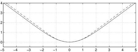
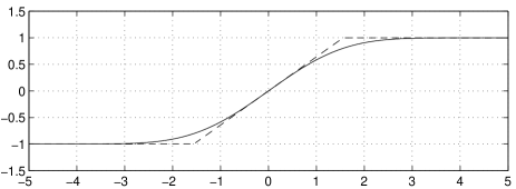
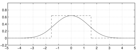
Figure 3: From top to bottom: potential function, first and second derivative. Solid line: Log-Erf potential $\varphi(x)$ of Eq. (6) and dotted line: corresponding Huber potential of Eq. (7). The potential parameters are $\gamma_{\mathrm{d}}=\gamma_{\mathrm{b}}=1$ and hence the equivalent Huber parameters are $\lambda\simeq 0.32$ and $s\simeq 1.56$, according to Eq. (8).

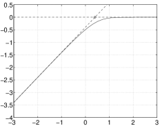
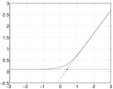
Figure 4: $\lambda$ and $s$ as a function of $\gamma_{\mathrm{b}}$, for a fixed $\gamma_{\mathrm{d}}$ ($\gamma_{\mathrm{d}}=1$) on a log-log scale. As expected, the plot essentially shows two linear behaviors and a critical case for $\gamma_{\mathrm{b}}=\sqrt{2\pi}$  ($\log_{10}\sqrt{2\pi}\sim 0.4$).

III-C Laplace Law for Auxiliary Variables

The following developments are dedicated to the case of auxiliary variables under a Laplace law suggested by [28].

As mentioned by [28] itself, among the Huber-like distributions, such a Laplace-convolved-Gauss probability will have two main advantages: ($i$) the convolution involved in the marginal law $f_{{\mathcal{X}}}$ (Section III-B) will be made explicit and ($ii$) the sampling of auxiliary variables (Section IV-C) will be directly feasible thanks to the inversion of the cumulative density function $F_{{\mathcal{B}}|{\mathcal{X}}}$.

The Laplace law is written in the form:

$$f_{{\mathcal{B}}}\left[{\mathb{B}}\right]=K_{{\mathcal{B}}}^{-1}~{}\exp\left[-\,\gamma_{\mathrm{b}}\,N_{1}({\mathb{B}})\,/2\right]\,,$$ (4)

where $\gamma_{\mathrm{b}}>0$ is a scale parameter, and $N_{1}({\mathb{B}})=\sum|b_{pq}|$ is the $\mbox{L}_{1}$ norm. The partition function is simply calculated thanks to separability

$$K_{{\mathcal{B}}}=\displaystyle\int_{{\mathbbm{R}}^{N}}\exp\left[-\,\gamma_{\mathrm{b}}\,N_{1}({\mathb{B}})\,/2\right]~{}{\mathrm{d}}{\mathb{B}}=\left[{\gamma_{\mathrm{b}}/4}\right]^{-N}\,.$$

According to (3) and (4) the joint density for $({\mathcal{X}},{\mathcal{B}})$ takes the form:

$$\begin{array}[]{l}{}\\ f_{{\mathcal{X}},{\mathcal{B}}}\left[{\mathb{X}},{\mathb{B}}\right]={}\\ {}\\ ~{}K_{{\mathcal{X}},{\mathcal{B}}}^{-1}\exp\left[-\,\gamma_{\mathrm{d}}\,N_{2}({\mathb{F}}\star{\mathb{X}}-{\mathb{B}})\,+\gamma_{\mathrm{b}}\,N_{1}({\mathb{B}})\,/2\right]{}\\ {}\\ \end{array}$$ (5)

and the partition function is explicit: $K_{{\mathcal{X}},{\mathcal{B}}}=K_{{\mathcal{X}}|{\mathcal{B}}}\,K_{{\mathcal{B}}}$.

The marginal law for ${\mathcal{X}}$ involves the one-dimensional convolution of a Gaussian density and a Laplacian density.

$$\begin{array}[]{l}{}\\ ~{}~{}f_{{\mathcal{X}}}\left[{\mathb{X}}\right]{}\\ {}\\ =\displaystyle K_{{\mathcal{X}},{\mathcal{B}}}^{-1}\prod_{pq}\int_{{\mathbbm{R}}}\exp\left[-\,\gamma_{\mathrm{d}}\,\left(\overline{x}_{pq}-b_{pq}\right)^{2}\,+\gamma_{\mathrm{b}}\,|b_{pq}|\,/2\right]~{}{\mathrm{d}}b_{pq}{}\\ {}\\ =\displaystyle K_{{\mathcal{X}},{\mathcal{B}}}^{-1}\prod_{pq}I(+\infty,\overline{x}_{pq},\gamma_{\mathrm{d}},\gamma_{\mathrm{b}}){}\\ \end{array}$$

where $I$ is defined in Appendix B. Thus, the potential function $\varphi$ appears:

$$f_{{\mathcal{X}}}\left[{\mathb{X}}\right]=K_{{\mathcal{X}},{\mathcal{B}}}^{-1}~{}~{}\exp\left[-\,\sum_{pq}\varphi(\overline{x}_{pq})\,/2\right]\,,$$

with:

$$\varphi(x)=-2\log I(+\infty,x,\gamma_{\mathrm{d}},\gamma_{\mathrm{b}})\,.$$ (6)

It is named the Log-Erf potential and it is shown in Fig. 3. The details of the calculations concerning this potential are given in Appendix C. Concerning the first derivative, one has:

$$\varphi^{\prime}(0)=0~{}~{}~{}\text{and\>}~{}~{}~{}\varphi^{\prime}(+\infty)=\gamma_{\mathrm{b}}\,,$$

and concerning the second derivative at origin, one has:

$$\varphi^{\prime\prime}(0) = \frac{\gamma_{\mathrm{b}}^{2}}{2}~{}\left[\left(\eta\,\sqrt{\pi}~{}\mathrm{erfcx}\left[\eta\right]\right)^{-1}-1\right]$$

with $\eta=\gamma_{\mathrm{b}}/\sqrt{8\gamma_{\mathrm{d}}}$ ($\mathrm{erfcx}\left[\cdot\right]$ is given in Appendix A). As expected (see Property 1), this is a convex potential. It is a $\mbox{L}_{2}-\mbox{L}_{1}$ potential which can be reconciled with other more common $\mbox{L}_{2}-\mbox{L}_{1}$ potentials (Huber, log-cosh, hyperbolic, fair function). In the case of the Huber potential:

$$x\mapsto\lambda~{}\begin{cases}x^{2}&\text{if\>}|\,x\,|\leq s\\ 2s\,|\,x\,|-s^{2}&\text{if\>}|\,x\,|\geq s\\ \end{cases}$$ (7)

by identifying the second derivatives at zero and the slopes at infinity, one has:

$$\lambda=\frac{1}{2}~{}\varphi^{\prime\prime}(0)~{}~{}~{}\text{and\>}~{}~{}~{}s=\frac{\varphi^{\prime}(+\infty)}{\varphi^{\prime\prime}(0)}\,.$$ (8)

Compared Log-Erf and Huber potentials and their derivatives are shown in Fig. 3. Using the expansions (14) and (13) of Appendix A, two limit cases can be identified, according to the value of the ratio $\eta$:

$$\begin{array}[]{lrclcrcl}\text{for\>}~{}\eta\gg 1:&\lambda&\simeq&\gamma_{\mathrm{d}}&;&s&\simeq&\displaystyle\frac{\gamma_{\mathrm{b}}}{2\,\gamma_{\mathrm{d}}}\\ {}\\ \text{for\>}~{}\eta\ll 1:&\lambda&\simeq&\displaystyle\gamma_{\mathrm{b}}\sqrt{\frac{\gamma_{\mathrm{d}}}{2\pi}}&;&s&\simeq&\displaystyle\sqrt{\frac{\pi}{2\,\gamma_{\mathrm{d}}}}\end{array}$$

In the two limit cases, on a log-log scale, there is linear behavior of $\lambda$ and $s$ as a function of $\gamma_{\mathrm{b}}$, for a fixed $\gamma_{\mathrm{d}}$ (see Fig. 4). The intersection of the two linear behaviors can be identified as a critical behavior for $\gamma_{\mathrm{b}}=\sqrt{2\pi\gamma_{\mathrm{d}}}$. The critical value will be used for the initialization of simulations of Section IV-D (see also Appendix H).

III-D Practical Case

In practice, the field is based on a $3\times 3$ Laplacian filter, defined by $[0\,,1\,,0\,;\,1\,,-4\,,1\,;\,0\,,1\,,0]$ and represented by the matrix ${\mathb{D}}$. At null frequency one has $\overset{\kern-3.30002pt~{}_{\circ}}{d}_{\scriptscriptstyle 00}=0$ and as a consequence the mean level of the image is not managed. So, an extra parameter is introduced to drive the mean level: it is denoted by $\varepsilon$ ($\varepsilon\geq 0$) and the characteristic matrix ${\mathb{F}}$ is set to ${\mathb{F}}_{\varepsilon}={\mathb{D}}+\varepsilon$.

Remark 3

— If $\varepsilon=0$ the field cannot be normalized and each clique is formed from the four nearest neighbors (cross-like clique). If $\varepsilon\neq 0$, the field can be normalized and each clique is spread out over the entire image.

The following developments take $\varepsilon>0$ and the partition function of the joint field writes:

$$K_{{\mathcal{X}},{\mathcal{B}}}^{-1}=\delta~{}\varepsilon~{}\gamma_{\mathrm{d}}^{\,N/2}~{}\gamma_{\mathrm{b}}^{\,N}\,,~{}~{}~{}~{}\text{with\>}~{}\delta=\left(32\pi\right)^{-N/2}\prod_{\stackrel{{\scriptstyle\scriptscriptstyle(p,q)}}{{\scriptscriptstyle\neq(0,0)}}}|\overset{\kern-3.30002pt~{}_{\circ}}{d}_{pq}|\,.$$

Fig. 1 gives a sample of the field with $\gamma_{\mathrm{d}}=\gamma_{\mathrm{b}}=1$ and Fig. 2 gives histograms of the image pixels, the auxiliary variables $B$ (a Laplace histogram) and the differences $\overline{X}$ (an over-Gaussian histogram).

Remark 4

— It is noteworthy that the marginal model ${\mathcal{X}}$ is homogeneous, but the conditional model ${\mathcal{X}}|{\mathcal{B}}$ is non-homogeneous (except if all the $b_{pq}$ are equal).

IV Deconvolution

As a result of the previous Section, a new random field is now available with a special feature: an explicit (and simple) partition function. In the present Section, the field serves as a prior in a deconvolution method whose specificity is to be unsupervised (i.e., including hyperparameter estimation). More precisely, the method relies on a full Bayesian framework and the solution is determined from an a posteriori law based on an a priori law (given below) for the object, the noise and the hyperparameters.

IV-A Prior choices

IV-A1 Object law

The a priori field is defined in the previous section. The joint density for $({\mathcal{X}},{\mathcal{B}})$ is given by (5) and it is driven by three parameters: $\gamma_{\mathrm{d}}$, $\gamma_{\mathrm{b}}$ and $\varepsilon$.

IV-A2 Noise law

The present work is founded on the usual case of zero-mean white Gaussian noise with inverse variance denoted $\gamma_{\mathrm{n}}$. The density is written:

$$f_{{\mathcal{N}}}({\mathb{N}})=\left(2\pi\right)^{-N/2}~{}~{}\gamma_{\mathrm{n}}^{N/2}\exp\left[-\,\gamma_{\mathrm{n}}~{}N_{2}({\mathb{N}})/2\right]\,.$$

IV-A3 Hyperparameter law

Four parameters are to be managed: $\gamma_{\mathrm{n}}$, $\gamma_{\mathrm{d}}$, $\gamma_{\mathrm{b}}$ and $\varepsilon$. The three parameters of major importance are ${\boldsymbol{\gamma}}=[\gamma_{\mathrm{n}},\gamma_{\mathrm{d}},\gamma_{\mathrm{b}}]$; the fourth parameter $\varepsilon$ drives the prior mean level of the image and it is considered as a nuisance parameter. Anyway, very few is a priori known about these parameters and the idea is to use non-informative or diffuse and separable priors.

• The proposed prior law for the three parameters $\gamma_{\mathrm{n}}$, $\gamma_{\mathrm{d}}$ and $\gamma_{\mathrm{b}}$ is a conjugate law. It is a gamma law (see Eq. (15), Appendix D) with parameters respectively denoted $(\alpha_{\mathrm{n}},\beta_{\mathrm{n}})$, $(\alpha_{\mathrm{d}},\beta_{\mathrm{d}})$ and $(\alpha_{\mathrm{b}},\beta_{\mathrm{b}})$. It allows for easy computations with the posterior law. Moreover, it includes diffuse and non-informative prior: the uniform prior and the Jeffrey’s prior are obtained as limit cases for $(\alpha,\beta)=(1,\infty)$ and for $(\alpha,\beta)=(0,\infty)$ respectively.

• The last parameter $\varepsilon$ is considered as a nuisance parameter and the proposed strategy resorts to integration out. The desired prior law is a Dirac law, so that no information is accounted for about the mean level of the image (it is set on the basis of observed data only). Formally, in a first step a uniform density over $[\,0,M_{\varepsilon}\,]$ is introduced and in a second step the limit law for $M_{\varepsilon}\rightarrow 0$ is considered.

IV-B Joint Law

Thus, the joint law is established for $({\mathcal{Y}},{\mathcal{X}},{\mathcal{B}},{\mathcal{C}},{\mathcal{E}})$:

$$\begin{array}[]{l}f_{{\mathcal{Y}},{\mathcal{X}},{\mathcal{B}},{\mathcal{C}},{\mathcal{E}}}({\mathb{Y}},{\mathb{X}},{\mathb{B}},{\boldsymbol{\gamma}},\varepsilon)~{}={}\\ {}\\ ~{}~{}~{}\delta^{\prime}~{}\gamma_{\mathrm{n}}^{~{}\alpha_{\mathrm{n}}-1+N/2}~{}\gamma_{\mathrm{d}}^{~{}\alpha_{\mathrm{d}}-1+N/2}~{}\gamma_{\mathrm{b}}^{~{}\alpha_{\mathrm{b}}-1+N}~{}\varepsilon~{}M_{\varepsilon}^{-1}{\mathbbm{1}}_{[\,0,M_{\varepsilon}\,]}(\varepsilon)\\ {}\\ ~{}~{}\exp-\,\left\{Q_{\varepsilon}/2~{}+~{}\gamma_{\mathrm{n}}/{\beta_{\mathrm{n}}}~{}+~{}\gamma_{\mathrm{d}}/{\beta_{\mathrm{d}}}~{}+~{}\gamma_{\mathrm{b}}/{\beta_{\mathrm{b}}}\right\}{}\\ {}\\ \end{array}$$

where $\delta^{\prime}=\left(2\pi\right)^{-N/2}\delta/\beta_{\mathrm{n}}^{\alpha_{\mathrm{n}}}\,\Gamma[\alpha_{\mathrm{n}}]~{}\beta_{\mathrm{b}}^{\alpha_{\mathrm{b}}}\,\Gamma[\alpha_{\mathrm{b}}]~{}\beta_{\mathrm{d}}^{\alpha_{\mathrm{d}}}\,\Gamma[\alpha_{\mathrm{d}}]$ is a normalization constant and $Q_{\varepsilon}$ is part of the Co-logarithm of the density involving ${\mathb{F}}_{\varepsilon}$:

$$Q_{\varepsilon}=\gamma_{\mathrm{n}}\,N_{2}({\mathb{Y}}-{\mathb{H}}\star{\mathb{X}})+\gamma_{\mathrm{d}}\,N_{2}({\mathb{F}}_{\varepsilon}\star{\mathb{X}}-{\mathb{B}})+\gamma_{\mathrm{b}}\,N_{1}({\mathb{B}})\,.$$

The a posteriori density is formed for ${\mathcal{X}}$, ${\mathcal{B}}$, ${\mathcal{C}}$ and ${\mathcal{E}}$, given ${\mathcal{Y}}$ thanks to the Bayes rule:

$$\begin{array}[]{l}f_{{\mathcal{X}},{\mathcal{B}},{\mathcal{C}},{\mathcal{E}}|{\mathcal{Y}}}({\mathb{X}},{\mathb{B}},{\boldsymbol{\gamma}},\varepsilon|{\mathb{Y}})={}\\ {}\\ ~{}~{}~{}~{}~{}~{}\displaystyle\frac{f_{{\mathcal{X}},{\mathcal{B}},{\mathcal{C}},{\mathcal{E}},{\mathcal{Y}}}({\mathb{X}},{\mathb{B}},{\boldsymbol{\gamma}},\varepsilon,{\mathb{Y}})}{\displaystyle\int_{{\mathb{X}},{\mathb{B}},{\boldsymbol{\gamma}},\varepsilon}f_{{\mathcal{X}},{\mathcal{B}},{\mathcal{C}},{\mathcal{E}},{\mathcal{Y}}}({\mathb{X}},{\mathb{B}},{\boldsymbol{\gamma}},\varepsilon,{\mathb{Y}})\,{\mathrm{d}}{\mathb{X}}\,{\mathrm{d}}{\mathb{B}}\,{\mathrm{d}}{\boldsymbol{\gamma}}\,{\mathrm{d}}\varepsilon}\,,\end{array}$$

and it is parametrized by the $(\alpha,\beta)$ and $M_{\varepsilon}$. Then, $\varepsilon$ is integrated out and the law for ${\mathcal{X}}$, ${\mathcal{B}}$, ${\mathcal{C}}$ given ${\mathcal{Y}}$ writes

$$f_{{\mathcal{X}},{\mathcal{B}},{\mathcal{C}}|{\mathcal{Y}}}({\mathb{X}},{\mathb{B}},{\boldsymbol{\gamma}}|{\mathb{Y}})=\displaystyle\int_{\varepsilon}f_{{\mathcal{X}},{\mathcal{B}},{\mathcal{C}},{\mathcal{E}}|{\mathcal{Y}}}({\mathb{X}},{\mathb{B}},{\boldsymbol{\gamma}},\varepsilon|{\mathb{Y}})\,{\mathrm{d}}\varepsilon\,.$$

It is also parametrized by the $(\alpha,\beta)$ and $M_{\varepsilon}$, so, the limit is set when $M_{\varepsilon}$ tends to 0. The detail of the calculations is given in Appendix E and it is shown that a probability density function is obtained if the mean level of the object is observed, i.e., $\overset{\kern-3.30002pt~{}_{\circ}}{h}_{\scriptscriptstyle 00}\neq 0$.

IV-C Posterior Law and Posterior Mean

Thus, the Total Posterior Law can be deduced for all the unknown parameters $({\mathcal{X}},{\mathcal{B}},{\mathcal{C}})$ given the observed data ${\mathcal{Y}}$:

$$\begin{array}[]{l}f_{{\mathcal{X}},{\mathcal{B}},{\mathcal{C}}|{\mathcal{Y}}}({\mathb{X}},{\mathb{B}},{\boldsymbol{\gamma}}|{\mathb{Y}})~{}\propto{}\\ {}\\ ~{}~{}~{}~{}~{}~{}\gamma_{\mathrm{n}}^{~{}\alpha_{\mathrm{n}}-1+N/2}~{}~{}\gamma_{\mathrm{d}}^{~{}\alpha_{\mathrm{d}}-1+N/2}~{}~{}\gamma_{\mathrm{b}}^{~{}\alpha_{\mathrm{b}}-1+N}{}\\ {}\\ ~{}~{}~{}~{}~{}\exp-\,\left\{Q_{0}/2~{}+~{}\gamma_{\mathrm{n}}/{\beta_{\mathrm{n}}}~{}+~{}\gamma_{\mathrm{d}}/{\beta_{\mathrm{d}}}~{}+~{}\gamma_{\mathrm{b}}/{\beta_{\mathrm{b}}}\right\}{}\\ {}\\ \end{array}$$ (9)

where $Q_{0}$ involves ${\mathb{F}}_{0}={\mathb{D}}$:

$$Q_{0}=\gamma_{\mathrm{n}}\,N_{2}({\mathb{Y}}-{\mathb{H}}\star{\mathb{X}})+\gamma_{\mathrm{d}}\,N_{2}({\mathb{D}}\star{\mathb{X}}-{\mathb{B}})+\gamma_{\mathrm{b}}\,N_{1}({\mathb{B}})\,.$$

In practice, the chosen point estimate is the posterior mean (i.e., the Minimum Mean Square Error). Its calculation is performed by means of Monte-Carlo Markov Chain stochastic sampling algorithm [33, 25]: auxiliary variables, object and hyperparameters are successively sampled given the other in a Gibbs strategy.

IV-C1 Sampling auxiliary variables

The sampling of auxiliary variables is delicate but can be directly done. It is based on the inversion of the cumulative density function (cdf) $F_{{\mathcal{B}}|{\mathcal{X}}}$. It is sufficient to uniformly sample $u$ in $[0,1]$ and to compute $b=F_{{\mathcal{B}}|{\mathcal{X}}}^{-1}(u)$. The calculations can be found in Appendix F.

IV-C2 Sampling object

The object is a toroidal Gaussian field and the $\overset{\kern-3.30002pt~{}_{\circ}}{X}_{pq}$ are independent with mean $\overset{\kern-3.30002pt~{}_{\circ}}{\mu}_{pq}$ and inverse variance $\overset{\kern-3.30002pt~{}_{\circ}}{\nu}_{pq}$ (see calculations in Appendix G)

$$\overset{\kern-3.30002pt~{}_{\circ}}{\nu}_{pq} = \gamma_{\mathrm{n}}\,|\overset{\kern-3.30002pt~{}_{\circ}}{h}_{pq}|^{2}+\gamma_{\mathrm{d}}\,|\overset{\kern-3.30002pt~{}_{\circ}}{d}_{pq}|^{2}$$ (10)

$$\overset{\kern-3.30002pt~{}_{\circ}}{\mu}_{pq} = \left[\,\gamma_{\mathrm{n}}\,\overset{\kern-3.30002pt~{}_{\circ}}{h}_{pq}^{\,*}~{}\overset{\kern-3.30002pt~{}_{\circ}}{y}_{pq}+\gamma_{\mathrm{d}}\,\overset{\kern-3.30002pt~{}_{\circ}}{d}_{pq}^{\,*}~{}\overset{\kern-3.30002pt~{}_{\circ}}{b}_{pq}\right]/\,\overset{\kern-3.30002pt~{}_{\circ}}{\nu}_{pq}$$ (11)

where superscript $~{}^{*}$ stands for the complex conjugate. Thus, the sampling is reduced to the sampling of an inhomogeneous white Gaussian noise followed by an fft-2d.

	Data	PM	CPM	CPM	CPM	CPM	MAP-LogErf	MAP-Huber
				(best $\gamma_{\mathrm{b}}$)	(best $\gamma_{\mathrm{d}}$)	(best $\gamma_{\mathrm{n}}$)
Dist. L2	11.62%	3.93%	3.94%	3.87%	3.85%	3.81%	5.56%	5.63%
Dist. L1	35.47%	19.47%	19.50%	18.92%	19.40%	19.18%	20.68%	20.84%

TABLE I: Quantitative comparison by means of L2 and L1 distances between true image and data (column 1), true image and estimated images (column 2 to 8).

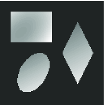
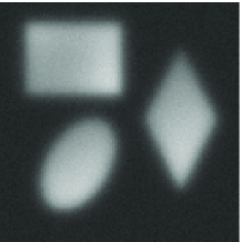
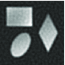
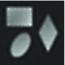
Figure 5: From left to right : original image ${\mathb{X}}^{\star}$, observed data ${\mathb{Y}}$, deconvolved image $\widehat{{\mathb{X}}}_{\textrm{PM}}$ and deconvolved image $\widehat{{\mathb{X}}}_{\textrm{MAP}}$. At the top: gray level images and at the bottom: profile of the 100-th row (which encroaches on both the rectangle and the rhombus). In order to evaluate the relative dynamics in each case, all the images are shown in the same gray-scale between -0.5 and 2. The four shown profiles are also presented between -0.5 and 2.

IV-C3 Sampling hyperparameters

Each parameter $\gamma_{\mathrm{n}}$, $\gamma_{\mathrm{d}}$ and $\gamma_{\mathrm{b}}$ follows a gamma law derived form (9) (see Appendix D) with respective parameters $\alpha$ and $\beta$

$$\begin{array}[]{lcl}\alpha=\alpha_{\mathrm{n}}+N/2&\text{and\>}&\beta^{-1}=\beta_{\mathrm{n}}^{-1}+{N_{2}({\mathb{Y}}-{\mathb{H}}\star{\mathb{X}})/2}\\ \alpha=\alpha_{\mathrm{d}}+N/2&\text{and\>}&\beta^{-1}=\beta_{\mathrm{d}}^{-1}+{N_{2}({\mathb{D}}\star{\mathb{X}}-{\mathb{B}})/2}\\ \alpha=\alpha_{\mathrm{b}}+N&\text{and\>}&\beta^{-1}=\beta_{\mathrm{b}}^{-1}+{N_{1}({\mathb{B}})/2}\,.\end{array}$$

The description of the method and the algorithm are now complete and synthesized in Table II. The remainder of this Section illustrates the implementation practicability.

Initialize • N = 1, Delta = inf • HatX = Data • GamN, GamD, GamB (Annex H)
Repeat • Sample step – Auxiliary variables B (Sect. IV-C1) – Object X (Sect. IV-C2) – Hyperparameter GamN,GamD,GamB (Sect. IV-C3) • Update – N = N+1 – Delta = ( HatX - X ) / N – HatX = ( (N-1)*HatX + 1*X ) / N Until Delta<eps

TABLE II: Detailed algorithm (pseudo-code).

IV-D Computation feasibility

This part illustrates the previous developments and it only aims at demonstrating the numerical practicability of the method. It is built on a deliberately simple image ${\mathb{X}}^{\star}$ appropriate in order to evaluate the capabilities and the limitations of the proposed approach: the image is set up from homogeneous zones separated by sharp edges (see Fig. 5, on the left). It is a $128\times 128$ image composed of a black background and three objects with gray levels gradually changing between 0.7 and 2.1. The difference between neighboring pixels varies between 0 and 2.1 in absolute value. Regarding the Laplacian of the image, $\overline{{\mathb{X}}}={\mathb{F}}\star{\mathb{X}}$, the set of $\overline{X}_{k}$ can be split in two sets: 94 % of the $\overline{X}_{k}$ are less than $2.10^{-4}$ (inside homogeneous zones) and 6 % of the $\overline{X}_{k}$ are greater than $3.10^{-2}$ (located around edges). No value is between $2.10^{-4}$ and $3.10^{-2}$.

The impulse response of the system is Gaussian shaped with 6 pixels width at half-maximum, the noise variance is $2.10^{-2}$ and the resulting observed image ${\mathb{Y}}$ is shown in Fig. 5 (in the second column). The resolution is clearly degraded and details of the edges are no longer visible (neither on the gray level image nor on the shown profile). The dynamic is also strongly affected, notably at about the 64-th sample of the shown profile.

The procedure is initialized by the empirical least-squares hyperparameters given in Appendix H. The object ${\mathb{X}}$ is initialized by the observed data (and there is no need to initialize the auxiliary variables). Moreover, practically, the $(\alpha_{*},\beta_{*})$ are set to $(0,\infty)$ corresponding to the Jeffrey’s prior.

The proposed algorithm generates samples of the a posteriori law $f_{{\mathcal{X}},{\mathcal{B}},{\mathcal{C}}|{\mathcal{Y}}}({\mathb{X}},{\mathb{B}},{\boldsymbol{\gamma}}|{\mathb{Y}})$. Practically, the algorithm behaves as expected: the stationary law is attained after a burn-in time (about 200 iterations) and remains in a steady behavior. The empirical mean of the generated images is recursively computed and the algorithm is stopped when its variation becomes smaller than a given value $T$ (in quadratic norm). In the presented example $T=5.10^{-4}$, the algorithm produced 953 iterations and computation time was 47 seconds.

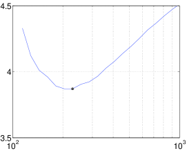
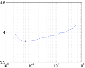
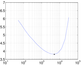
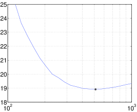
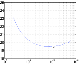
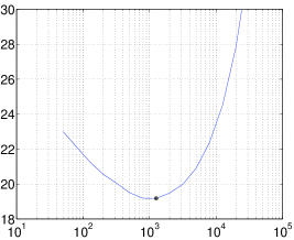
Figure 6: Distances between the true image ${\mathb{X}}^{\star}$ and Conditional Posterior Mean $\widehat{{\mathb{X}}}_{\textrm{CPM}}$ as a function of the parameters $\gamma_{\mathrm{b}}$, $\gamma_{\mathrm{d}}$ and $\gamma_{\mathrm{n}}$, around the posterior mean value $\widehat{{\boldsymbol{\gamma}}}$. From left to right: error is shown as a function of $\gamma_{\mathrm{b}}$, $\gamma_{\mathrm{d}}$ and $\gamma_{\mathrm{n}}$. Top row gives L2 distance and bottom row gives L1 distances. The black dots give the minimum distances reported in Table I.

The resulting generated hyperparameters $\gamma_{\mathrm{b}}$, $\gamma_{\mathrm{d}}$ and $\gamma_{\mathrm{n}}$ are shown in Fig. 7. The left part of the figure shows the 953 iterates of the three parameters: after about 200 iterations the three parameters are stabilized and seem to be under the stationary law of the chain. The empirical mean value (approximating the Posterior Mean) of the parameters respectively are $\widehat{\gamma_{\mathrm{b}}}=2.88\,10^{2}$, $\widehat{\gamma_{\mathrm{d}}}=5.91\,10^{4}$ and $\widehat{\gamma_{\mathrm{n}}}=1.99\,10^{3}$. The iterates are also shown on the right hand side of Fig. 7 as histograms: they are clearly very concentrated around the Posterior Mean (with small variance), i.e., the marginal law for the hyperparameters are quasi-Dirac distributions.

Considering the numerical value, in the sense of Eq. (8), the equivalent regularization parameter is $\widehat{\lambda}=2.17\,10^{1}$ and the equivalent threshold is $\widehat{s}=6.67\,10^{-3}$. It is noticeable that the threshold value correctly split the $\overline{X}_{k}$ in two sets (less than $2.10^{-4}$ – greater than $3.10^{-2}$). The point is that the method automatically adjusts hyperparameters to correctly separate the $\overline{X}_{k}$. This is a first argument in favor of the proposed strategy in order to tune the threshold of an $\mbox{L}_{2}-\mbox{L}_{1}$ Gibbs potential.

The resulting image is shown in Fig. 5 (on the third column). The effect of deconvolution is notable on the image in gray level as well as on the shown profile. The three objects are correctly positioned, the orders of magnitude are respected and the zero level is correctly reconstructed: it can be seen on the entire image and in particular on the shown profile. The dynamic is also correctly restored: this aspect is notable on the shown profile around the maximum (64-th sample). The true dynamic occupies the range 0 – 1.9 whereas the dynamic of the observed data scarcely exceeds 0 – 1.4: the proposed method restores the dynamic to 0 – 1.88 that is to say 99% of the original variation.

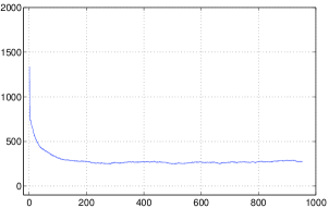
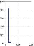
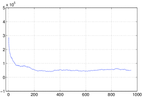
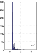
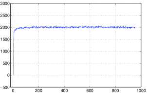
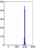
Figure 7: Monte-Carlo Markov Chain for the three hyperparameters generated by the proposed Gibbs sampler. From top to bottom: $\gamma_{\mathrm{b}}$, $\gamma_{\mathrm{d}}$ and $\gamma_{\mathrm{n}}$. The left part of the figure shows the samples as a function of iteration index and the right part of the figure shows the samples as histograms.

A global quantitative comparison has been achieved by evaluating ($i$) the distance between original image ${\mathb{X}}^{\star}$ and observed data ${\mathb{Y}}$ and ($ii$) the distance between original image ${\mathb{X}}^{\star}$ and estimated image $\widehat{{\mathb{X}}}_{\textrm{PM}}$. The considered distances are normalized L2 and L1 distances. The main results are listed in Table I, first and second columns and show an improvement by a factor 2.95 (11.62% to 3.93%) for L2 distance and a factor 1.82 (35.47% to 19.47%) for L1 distance.

In order to deepen the numerical study, a second estimate has been computed: $\widehat{{\mathb{X}}}_{\textrm{CPM}}$ the Conditional Posterior Mean (CPM), i.e., the mean of the conditional posterior law $f_{{\mathcal{X}},{\mathcal{B}}|{\mathcal{Y}},{\mathcal{C}}}({\mathb{X}},{\mathb{B}}|{\mathb{Y}},{\boldsymbol{\gamma}})$. $\widehat{{\mathb{X}}}_{\textrm{CPM}}$ is clearly a function of the hyperparameters ${\boldsymbol{\gamma}}$ and a twofold evaluation is proposed.

• The first estimate is the one obtained with ${\boldsymbol{\gamma}}=\widehat{{\boldsymbol{\gamma}}}$. Practically, the marginal estimate $\widehat{{\mathb{X}}}_{\textrm{PM}}$ and the conditional estimate $\widehat{{\mathb{X}}}_{\textrm{CPM}}(\widehat{{\boldsymbol{\gamma}}})$ are quasi-equal; this is due to the fact that the marginal law for the hyperparameters are quasi-Dirac distributions. Quantitatively, regarding L2 distances, the PM produces 3.93% whereas the CPM produces 3.94%; regarding L1 distances, the PM produces 19.47% whereas the CPM produces 19.50%. In both cases, the modification is almost imperceptible.

• The measurement of errors has also been explored for the CPM as a function $\gamma_{\mathrm{b}}$, $\gamma_{\mathrm{d}}$ and $\gamma_{\mathrm{n}}$, around the posterior mean $\widehat{{\boldsymbol{\gamma}}}$. Results are given on Fig. 6: in each case, smooth variation of distances is observed when varying parameters and an optimum is visible. It is reported on Table I and shows almost imperceptible modification: optimization of the hyperparameters (based on the true image ${\mathb{X}}^{\star}$) allows negligible improvement (smaller than 0.1% for L2 error and smaller than 0.5% for L1 error). So, the main conclusion is that, the unsupervised proposed approach is a relevant tool in order to tune parameters: it works (without the knowledge of the true image) as well as an optimized approach (based on the knowledge of the true image).

Finally, a third estimate has been computed: the Maximum A posteriori (MAP). It has been computed for the LogErf and the Huber potentials. Both of them have been computed with equivalent hyperparameters (given above): $(\widehat{\gamma_{\mathrm{b}}},\widehat{\gamma_{\mathrm{d}}},\widehat{\gamma_{\mathrm{n}}})$ for the LogErf potential and $(\widehat{\lambda},\widehat{s})$ for the Huber potential. The two MAP solutions (LogErf and Huber) are visually indiscernible: this is expected from so similar potential. The results are presented in Fig. 5, right column: the estimated map suffers from cross-like artifact, due to the cross-like structure of the neighborhood system. Quantitatively speaking, the measurements of errors are given on Table I: LogErf and Huber produce almost similar errors. Moreover, the errors are greater than the one produced by the PM and the CPM.

The restoration is nevertheless imperfect and of limited resolution: the sharp edges remain slightly smoothed and limited in amplitude. The ringing effect also affects the quality of the deconvolved image. This diagnostic is long awaited in the framework of convex deconvolution. Anyway, the important point is not so much the property of the deconvolved image itself (intrinsic of any convex deconvolution) but the (new) practical capability to automatically tune the hyperparameters. Moreover, the potential improvement is certainly wide considering more heavy-tailed law for the auxiliary variables, as explained in the next section.

V Conclusion

This paper presents a twofold novelty in the field of statistical image reconstruction and restoration.

1. The partition function is explicitly given for a specific non-Gaussian Markov field, with an $\mbox{L}_{2}-\mbox{L}_{1}$ Gibbs potential. It is built as a compound field involving: an auxiliary variable following a separable Laplace distribution and a pixel variable following a Gaussian distribution given the auxiliary variable.

2. An unsupervised deconvolution method is deduced, based on the exact likelihood taking advantage of the knowledge of the partition function. The method is fully Bayesian, and the point estimate is the posterior mean computed thanks to a Monte-Carlo Markov Chain technique.

The paper focuses on the deconvolution problem, but it is also possible to deal with simpler questions than deconvolution: parameter estimation from direct observation of the field, edge enhancement or denoising.

Moreover, the paper relies on Gaussian noise, but the case of non-Gaussian noise is also envisaged, in particular the use of robust norms to reject abnormal data (outliers). To this end, a separable version of the $\mbox{L}_{2}-\mbox{L}_{1}$ proposed field could be suitable as a law for noise measurement.

The proposed method can be directly applied in the case of large support operator, e.g., reconstruction problems such as Fourier synthesis [34]. The proposed methodology also remains valid for other linear model and the required modification concerns the sampling of the object. It remains Gaussian but its sampling is no longer possible in a single step for the entire image by fft-2d. The Gibbs sampling techniques constitute an adapted tool but the calculation time would be (maybe dramatically) extended. For non-linear problems, the law for the object is no longer Gaussian and a case by case study is required.

Concerning the a priori field, other laws for auxiliary variables are certainly desirable. The possible improvements are numerous considering more heavy-tailed law in order to overcome the limitation of the convex deconvolution. The methodology still remains valid but the difficulty then concerns the sampling of the auxiliary variables. The direct sampling by inversion of the cumulative density function may not be possible, however, the rejection or the Hastings-Metropolis algorithms could be used to overcome this difficulty.

In the case of myopic deconvolution, it is also conceivable to estimate (part of) the parameters of the observation system. Here again, a case by case study is necessary, but the delicate question of the system parameter sampling can probably be tackled by means of rejection or Hastings-Metropolis algorithms.

Appendix A erf, erfc, erfcx

The $\mathrm{erf}$ function is defined for $x\in{\mathbbm{R}}$ by:

$$\mathrm{erf}\left[x\right]=\frac{2}{\sqrt{\pi}}\int_{0}^{x}\exp\left[-t^{2}\right]\,{\mathrm{d}}t\,,$$ (12)

and $\mathrm{ierf}$ denotes the reciprocal function. Elsewhere, $\mathrm{erfc}\left[x\right]=1-\mathrm{erf}\left[x\right]$ and $\mathrm{erfcx}\left[x\right]=\exp\left[x^{2}\right]\mathrm{erfc}\left[x\right]$. Concerning the latter, there are the following expansions:

$$\mathrm{erfcx}\left[x\right] \underset{+\infty}{\sim} \left[1-x^{-2}\right]/\left(x\sqrt{\pi}\right)$$ (13)

$$\mathrm{erfcx}\left[x\right] \underset{0}{\sim} 1-{2x/\sqrt{\pi}}\,.$$ (14)

and the derivative $\mathrm{erfcx}\left[x\right]^{\prime}=2\,x\,\mathrm{erfcx}\left[x\right]-2/\sqrt{\pi}$.

Appendix B Gauss and Laplace convolution

Considering the calculations, a large part of the proposed developments is based on the convolution of a Gaussian function and a Laplacian function.

B-A Preliminary Calculi

For $x_{0}\geq 0$ and $x\in{\mathbbm{R}}$, write:

$$J(x_{0},x,d,b)=\int_{0}^{x_{0}}\exp\left[-\left\{d(y-x)^{2}+by\right\}/2\right]~{}{\mathrm{d}}y\,,$$

simply written as $J(x_{0},x)$ when there is no ambiguity. On rewriting the argument of the exponential, we have:

$$d(y-x)^{2}+by=d\left[(y-\tilde{x})^{2}+(x^{2}-\tilde{x})^{2}\right]$$

with $\tilde{x}=x-b/2d$. The change of variable $t=(y-\tilde{x})\,\sqrt{d/2}$, yields:

$$J(x_{0},x) = \sqrt{{\pi/2d}}~{}\exp\left[{b^{2}/8d}\right]~{}\exp\left[-bx/2\right]$$

$$\left\{\mathrm{erf}\left[\tilde{x}~{}\sqrt{{d/2}}\right]-\mathrm{erf}\left[(\tilde{x}-x_{0})~{}\sqrt{{d/2}}\right]\right\}\,,$$

where the function $\mathrm{erf}$ is defined by (12). In particular, one has: $J(0,x)=0$ and

$$J(+\infty,x) = \sqrt{{\pi/2d}}~{}\exp\left[{b^{2}/8d}\right]~{}$$

$$\exp\left[-bx/2\right]~{}\mathrm{erfc}\left[-\tilde{x}~{}\sqrt{{d/2}}\right]\,.$$

B-B Convolution

For $x_{0},x\in{\mathbbm{R}}$, write:

$$I(x_{0},x,d,b)=\int_{-\infty}^{x_{0}}\exp\left[-\left\{d(y-x)^{2}+b|y|\right\}/2\right]~{}{\mathrm{d}}y\,,$$

written simply as $I(x_{0},x)$ when there is no ambiguity. By the change of variables $y^{\prime}=-y$, $y^{\prime}=by$, and $y^{\prime}=y\sqrt{d}$, it is shown that:

$$I(+\infty,x,d,b) = I(+\infty,-x,d,b)$$

$$I(x_{0},x,d,b) = I(bx_{0},bx,d/b^{2},1)\,/\,b$$

$$I(x_{0},x,d,b) = I(x_{0}\sqrt{d},x\sqrt{d},1,b/\sqrt{d})\,/\,\sqrt{d}$$

It can thus be deduced that:

$$I(x_{0},x,d,b) = J(+\infty,-x,d,b)-J(-x_{0},-x,d,b)$$

$$I(x_{0},x,d,b) = J(+\infty,-x,d,b)+J(x_{0},x,d,b)$$

respectively for $x_{0}<0$ and $x_{0}\geq 0$. These relationships are useful for the study of the potential function (next Appendix) and for the inversion of the cdf of ${\mathcal{B}}|{\mathcal{X}}$ (Appendix F).

Appendix C Log-Erf Potential function

According to the results of the previous Appendix the potential function of the marginal field ${\mathcal{X}}$, Eq. (6), Section III-C is written:

$$\varphi(x)=-2\log I(+\infty,x,\gamma_{\mathrm{d}},\gamma_{\mathrm{b}})\,.$$

By putting: $\chi(x)=\exp\left[\gamma_{\mathrm{b}}\,x/2\right]~{}\mathrm{erfc}\left[(\rho+x)~{}\sqrt{{\gamma_{\mathrm{d}}/2}}\right]$, $\rho=\gamma_{\mathrm{b}}/2\gamma_{\mathrm{d}}$ the potential function can be written:

$$\varphi(x)=-2\log\left[\chi(x)+\chi(-x)\right]\,,$$

up to additive constants. The derivation shows that :

$$\chi^{\prime}(x) = \frac{\gamma_{\mathrm{b}}}{2}\,\chi(x)-\sqrt{\frac{2\,\gamma_{\mathrm{d}}}{\pi}}\,\exp\left[-\gamma_{\mathrm{d}}\left(\rho^{2}+x^{2}\right)/2\right]$$

$$\chi^{\prime\prime}(x) = \frac{\gamma_{\mathrm{b}}}{2}\,\chi^{\prime}(x)+\sqrt{\frac{2\,\gamma_{\mathrm{d}}^{3}}{\pi}}\,x\,\exp\left[-\gamma_{\mathrm{d}}\left(\rho^{2}+x^{2}\right)/2\right]$$

and it can easily be deduced that:

$$\varphi^{\prime}(x)=-2~{}\frac{\chi^{\prime}(x)-\chi^{\prime}(-x)}{\chi(x)+\chi(-x)}=-\gamma_{\mathrm{b}}~{}\frac{\chi(x)-\chi(-x)}{\chi(x)+\chi(-x)}$$

and in particular

$$\varphi^{\prime}(0)=0~{}~{}~{}\text{and\>}~{}~{}~{}\varphi^{\prime}(+\infty)=\gamma_{\mathrm{b}}\,.$$

Moreover, concerning the second derivative at origin

$$\varphi^{\prime\prime}(0) = -\,2~{}\frac{\chi^{\prime\prime}(0)}{\chi(0)}=-\,\gamma_{\mathrm{b}}~{}\frac{\chi^{\prime}(0)}{\chi(0)}$$

$$= \frac{\gamma_{\mathrm{b}}^{2}}{2}~{}\left[\left(\eta\,\sqrt{\pi}~{}\mathrm{erfcx}\left[\eta\right]\right)^{-1}-1\right]$$

with $\eta=\gamma_{\mathrm{b}}/\sqrt{8\gamma_{\mathrm{d}}}$.

Appendix D Gamma Probability Density Function

The gamma probability density function is parametrized by $\alpha>0$ and $\beta>0$ in the form:

$$f_{\gamma}\left(x\,;\,\alpha,\beta\right)=\frac{1}{\beta^{\alpha}\,\Gamma[\alpha]}~{}x^{\alpha-1}~{}\exp\left[-x/\beta\right]\,\,{\mathbbm{1}}_{{\mathbbm{R}}_{+}}(x)\,,$$ (15)

where ${\mathbbm{1}}_{{\mathbbm{R}}_{+}}$ is the indicator function of ${\mathbbm{R}}_{+}$. The expected value is $\alpha\,\beta$, the variance is $\alpha\,\beta^{2}$ and it is maximal for $x=\beta(\alpha-1)$ in the case $\alpha>1$.

Appendix E Integration of Hyperparameter

E-A Preliminary Result

Given a function $f:{\mathbbm{R}}\rightarrow{\mathbbm{R}}_{+}$, ${\mathcal{C}}^{\infty}$ and assume that $g(x)=xf(x)$ can be integrated. By integrating from $0$ to $M$ the Taylor expansion of $g(x)$ at origin, one shows that:

$$\frac{1}{M^{2}}~{}\int_{0}^{M}x\,f(x)\,{\mathrm{d}}x\underset{\scriptscriptstyle M=0}{\longrightarrow}\frac{1}{2}~{}f(0)\,.$$ (16)

Then, give a function $\psi:{\mathbbm{R}}^{Q}\times{\mathbbm{R}}\rightarrow{\mathbbm{R}}_{+}$ such that $\varepsilon\,\psi({\mathb{u}},\varepsilon)$ can be integrated over ${\mathbbm{R}}^{Q+1}$. By using (16), it can be seen that:

$$\frac{\displaystyle\int_{0}^{M}\varepsilon~{}\psi({\mathb{u}},\varepsilon)\,{\mathrm{d}}\varepsilon}{\displaystyle\int_{\mathb{v}}\int_{0}^{M}\eta~{}\psi({\mathb{v}},\eta)\,{\mathrm{d}}\eta\,{\mathrm{d}}{\mathb{v}}}~{}\underset{\scriptscriptstyle M=0}{\longrightarrow}\frac{\psi({\mathb{u}},0)}{\displaystyle\int_{\mathb{v}}\psi({\mathb{v}},0)\ {\mathrm{d}}{\mathb{v}}}~{}$$ (17)

provided that $\psi({\mathb{v}},0)$ can still be integrated over ${\mathbbm{R}}^{Q}$.

E-B Posterior Law

The a posteriori law (Section IV-B) for ${\mathcal{X}}$, ${\mathcal{B}}$, ${\mathcal{C}}$ and ${\mathcal{E}}$ given ${\mathcal{Y}}$ (parametrized by the coefficient $M_{\varepsilon}$) is written, after simplification by $\delta^{\prime}M_{\varepsilon}$:

$$\frac{\displaystyle\int_{\varepsilon=0}^{M_{\varepsilon}}\psi({\mathb{u}},\varepsilon)~{}{\mathrm{d}}\varepsilon}{\displaystyle\int_{{\mathb{X}}{\mathb{B}}{\boldsymbol{\gamma}}}\int_{\varepsilon=0}^{M_{\varepsilon}}\psi({\mathb{v}},\varepsilon)~{}{\mathrm{d}}\varepsilon~{}{\mathrm{d}}{\boldsymbol{\gamma}}~{}{\mathrm{d}}{\mathb{X}}~{}{\mathrm{d}}{\mathb{B}}}$$

where ${\mathb{u}}$ represents all the parameters ${\mathb{X}},{\mathb{B}},{\boldsymbol{\gamma}}$ and:

$$\begin{array}[]{l}\psi({\mathb{u}},\varepsilon)~{}=\delta^{\prime}~{}\gamma_{\mathrm{n}}^{~{}\alpha_{\mathrm{n}}-1+N/2}~{}~{}\gamma_{\mathrm{d}}^{~{}\alpha_{\mathrm{d}}-1+N/2}~{}~{}\gamma_{\mathrm{b}}^{~{}\alpha_{\mathrm{b}}-1+N}~{}\varepsilon{}{}{}{}{}{}\\ {}\\ ~{}~{}~{}~{}~{}~{}~{}~{}\exp-\,\left\{Q_{\varepsilon}/2~{}+~{}\gamma_{\mathrm{n}}/{\beta_{\mathrm{n}}}~{}+~{}\gamma_{\mathrm{d}}/{\beta_{\mathrm{d}}}~{}+~{}\gamma_{\mathrm{b}}/{\beta_{\mathrm{b}}}\right\}\,.{}\\ {}\\ \end{array}$$

To apply the relationship (17), it is sufficient to ensure that $\psi({\mathb{v}},0)$ can be integrated. Since the norms in ${\mathbbm{R}}^{N}$ are equivalent, $k\in{\mathbbm{R}}_{+}$ can be found such as $N_{1}({\mathb{B}})<kN_{2}({\mathb{B}})$ for all ${\mathb{B}}$. Thus the integrand can be majored by a Gaussian integrand and convergence ensured if and only if $\overset{\kern-3.30002pt~{}_{\circ}}{h}_{\scriptscriptstyle 00}\neq 0$.

In the limit, when $M_{\varepsilon}\rightarrow 0$, we have the result (9).

Appendix F Inversion of ${\mathcal{B}}|{\mathcal{X}}$ cdf

The sampling of auxiliary variables (Section IV-C) given the object is based on the inversion of cdf of ${\mathcal{B}}|{\mathcal{X}}$. For $u\in[0,1]$:

$$u=F_{{\mathcal{B}}|{\mathcal{X}}}(b)=\int_{-\infty}^{b}f_{{\mathcal{B}}|{\mathcal{X}}}=\frac{I(b,\bar{b},\gamma_{\mathrm{d}},\gamma_{\mathrm{b}})}{I(+\infty,\bar{b},\gamma_{\mathrm{d}},\gamma_{\mathrm{b}})}\,.$$ (18)

is to be resolved. In order to solve this equation, write $\rho=\gamma_{\mathrm{b}}/2\gamma_{\mathrm{d}}$

$$\theta_{-} = \exp\left[+\gamma_{\mathrm{b}}\,\bar{b}/2\right]~{}\mathrm{erfc}\left[(\rho+\bar{b})~{}\sqrt{{\gamma_{\mathrm{d}}/2}}\right]$$

$$\theta_{+} = \exp\left[-\gamma_{\mathrm{b}}\,\bar{b}/2\right]~{}\mathrm{erfc}\left[(\rho-\bar{b})~{}\sqrt{{\gamma_{\mathrm{d}}/2}}\right]$$

and $\theta=\theta_{-}+\theta_{+}$. Moreover $s=F_{{\mathcal{B}}|{\mathcal{X}}}(0)=\theta_{-}/\theta$ and $\bar{u}=\theta u-\theta_{-}$. Equation (18) is resolved differently depending on whether $u\leq s$ (i.e., $b\leq 0$) or $u\geq s$ (i.e., $b\geq 0$) and yields:

$$b=\bar{b}+\rho-\mathrm{ierf}\left\{T_{-}\right\}\sqrt{2/\gamma_{\mathrm{d}}} u\leq s$$ if

$$b=\bar{b}-\rho-\mathrm{ierf}\left\{T_{+}\right\}\sqrt{2/\gamma_{\mathrm{d}}} u\geq s$$ if

where $\mathrm{ierf}\left\{\cdot\right\}$ is defined in Appendix A and

$$T_{-} = \mathrm{erf}\left[(\bar{b}+\rho)~{}\sqrt{{\gamma_{\mathrm{d}}/2}}\right]-\bar{u}~{}\exp\left[-\gamma_{\mathrm{b}}\,\bar{b}/2\right]$$

$$T_{+} = \mathrm{erf}\left[(\bar{b}-\rho)~{}\sqrt{{\gamma_{\mathrm{d}}/2}}\right]-\bar{u}~{}\exp\left[+\gamma_{\mathrm{b}}\,\bar{b}/2\right]\,.$$

Thus it is possible to sample ${\mathcal{B}}|{\mathcal{X}}$ simply from $u$ uniformly distributed over $[0,1]$.

Appendix G Conditional posterior law for ${\mathcal{X}}$

The posterior law $({\mathcal{X}},{\mathcal{B}},{\mathcal{C}}|{\mathcal{Y}}$) given by Eq. (9) in Section IV-C involves

$$Q_{0}=\gamma_{\mathrm{n}}\,N_{2}({\mathb{Y}}-{\mathb{H}}\star{\mathb{X}})+\gamma_{\mathrm{d}}\,N_{2}({\mathb{D}}\star{\mathb{X}}-{\mathb{B}})+\gamma_{\mathrm{b}}\,N_{1}({\mathb{B}})\,,$$

and the conditional posterior law $({\mathcal{X}}|{\mathcal{B}},{\mathcal{C}},{\mathcal{Y}}$) required to sample object in Section IV-C2 involves

$$Q_{0|}=\gamma_{\mathrm{n}}\,N_{2}({\mathb{Y}}-{\mathb{H}}\star{\mathb{X}})+\gamma_{\mathrm{d}}\,N_{2}({\mathb{D}}\star{\mathb{X}}-{\mathb{B}})\,.$$

In the Fourier domain:

$$Q_{0|} = \gamma_{\mathrm{n}}\,N_{2}(\overset{\kern-3.30002pt~{}_{\circ}}{{\mathb{Y}}}-\overset{\kern-3.30002pt~{}_{\circ}}{{\mathb{H}}}\otimes\overset{\kern-3.30002pt~{}_{\circ}}{{\mathb{X}}})+\gamma_{\mathrm{d}}\,N_{2}(\overset{\kern-3.30002pt~{}_{\circ}}{{\mathb{D}}}\otimes\overset{\kern-3.30002pt~{}_{\circ}}{{\mathb{X}}}-\overset{\kern-3.30002pt~{}_{\circ}}{{\mathb{B}}})$$

$$= \sum_{pq}\gamma_{\mathrm{n}}\,|\overset{\kern-3.30002pt~{}_{\circ}}{y}_{pq}-\overset{\kern-3.30002pt~{}_{\circ}}{h}_{pq}\overset{\kern-3.30002pt~{}_{\circ}}{x}_{pq}|^{2}+\gamma_{\mathrm{d}}\,|\overset{\kern-3.30002pt~{}_{\circ}}{d}_{pq}\overset{\kern-3.30002pt~{}_{\circ}}{x}_{pq}-\overset{\kern-3.30002pt~{}_{\circ}}{b}_{pq}|^{2}$$

that is to say a separable summation. Moreover, it can be rewritten and identified to a sum of quadratic terms:

$$Q_{0|} = \sum_{pq}\overset{\kern-3.30002pt~{}_{\circ}}{\nu}_{pq}|\overset{\kern-3.30002pt~{}_{\circ}}{x}_{pq}-\overset{\kern-3.30002pt~{}_{\circ}}{\mu}_{pq}|^{2}$$

with $\overset{\kern-3.30002pt~{}_{\circ}}{\nu}_{pq}$ and $\overset{\kern-3.30002pt~{}_{\circ}}{\mu}_{pq}$ given in Eq. (10) - (11).

Appendix H Empirical Least Squares Hyperparameters

The initialization of the algorithm is based on second order statistics of the analyzed data, in the Fourier domain. Considering the structure of the a priori field and the noise, for all $(p,q)$, such as $\overset{\kern-3.30002pt~{}_{\circ}}{f}_{pq}\neq 0$ one has:

$$\overset{\kern-3.30002pt~{}_{\circ}}{X}_{pq}=\sqrt{r_{\mathrm{d}}}~{}\overset{\kern-3.30002pt~{}_{\circ}}{G}_{pq}/\overset{\kern-3.30002pt~{}_{\circ}}{f}_{pq}~{}~{}~{}\text{and\>}~{}~{}~{}\overset{\kern-3.30002pt~{}_{\circ}}{N}_{pq}=\sqrt{r_{\mathrm{n}}}~{}\overset{\kern-3.30002pt~{}_{\circ}}{G}^{\prime}_{pq}\\$$

where $\overset{\kern-3.30002pt~{}_{\circ}}{G}_{pq}$ and $\overset{\kern-3.30002pt~{}_{\circ}}{G}^{\prime}_{pq}$ are two independent zero-mean white Gaussian noise with unitary variance. Moreover, considering the observation equation (1), one also has $\overset{\kern-3.30002pt~{}_{\circ}}{Y}_{pq}=\overset{\kern-3.30002pt~{}_{\circ}}{h}_{pq}\overset{\kern-3.30002pt~{}_{\circ}}{X}_{pq}+\overset{\kern-3.30002pt~{}_{\circ}}{N}_{pq}$. With $\overset{\kern-3.30002pt~{}_{\circ}}{Z}_{pq}=|\overset{\kern-3.30002pt~{}_{\circ}}{Y}_{pq}|^{2}$ and $\overset{\kern-3.30002pt~{}_{\circ}}{r}_{pq}=|\overset{\kern-3.30002pt~{}_{\circ}}{h}_{pq}|/|\overset{\kern-3.30002pt~{}_{\circ}}{f}_{pq}|$, we have:

$${\mathrm{E}}\bigl{[}\overset{\kern-3.30002pt~{}_{\circ}}{Z}_{pq}\bigr{]}=r_{\mathrm{d}}~{}\overset{\kern-3.30002pt~{}_{\circ}}{r}_{pq}+r_{\mathrm{n}}\,.$$

Thus the parameters $r_{\mathrm{d}}$ and $r_{\mathrm{n}}$ can be selected at the minimum of the least squares criterion:

$$J(r_{\mathrm{d}},r_{\mathrm{n}})=\sum_{pq}(\overset{\kern-3.30002pt~{}_{\circ}}{z}_{pq}-r_{\mathrm{d}}~{}\overset{\kern-3.30002pt~{}_{\circ}}{r}_{pq}+r_{\mathrm{n}})^{2}\,.$$

It is found that:

$$r_{\mathrm{d}}=\frac{\gamma-\alpha\delta}{\beta-\alpha^{2}}~{}~{}~{}\text{and\>}~{}r_{\mathrm{n}}=\frac{\beta\delta-\alpha\gamma}{\beta-\alpha^{2}}$$

with $N\alpha=\sum\overset{\kern-3.30002pt~{}_{\circ}}{r}_{pq}$, $N\beta=\sum\overset{\kern-3.30002pt~{}_{\circ}}{r}_{pq}^{2}$, $N\gamma=\sum\overset{\kern-3.30002pt~{}_{\circ}}{r}_{pq}\overset{\kern-3.30002pt~{}_{\circ}}{z}_{pq}$, and $N\delta=\sum\overset{\kern-3.30002pt~{}_{\circ}}{z}_{pq}$. These values for $r_{\mathrm{d}}$ and $r_{\mathrm{n}}$ are used to initialize the proposed algorithm (Section IV-C): $\gamma_{\mathrm{d}}=1/r_{\mathrm{d}}$ and $\gamma_{\mathrm{n}}=1/r_{\mathrm{n}}$. The third parameter $\gamma_{\mathrm{b}}$ is initialized at the critical value: $\gamma_{\mathrm{b}}=\sqrt{2\pi\gamma_{\mathrm{d}}}$.

Jean-François Giovannelli was born in Béziers, France, in 1966. He graduated from the École Nationale Supérieure de l’Électronique et de ses Applications in 1990. He received the Doctorat degree in physics at Université Paris-Sud, Orsay, France, in 1995. He is presently assistant professor in the Département de Physique at Université Paris-Sud and researcher with the Laboratoire des Signaux et Systèmes (CNRS - Supélec - UPS). He is interested in regularization and Bayesian methods for inverse problems in signal and image processing. Application fields essentially concern astronomical, medical and geophysical imaging.

References

- [1] A. Tikhonov and V. Arsenin, Solutions of Ill-Posed Problems. Washington, dc: Winston, 1977.
- [2] H. C. Andrews and B. R. Hunt, Digital Image Restoration. Englewood Cliffs, nj: Prentice-Hall, 1977.
- [3] S. Geman and D. Geman, “Stochastic relaxation, Gibbs distributions, and the Bayesian restoration of images,” IEEE Trans. Pattern Anal. Mach. Intell., vol. 6, no. 6, pp. 721–741, November 1984.
- [4] A. Blake and A. Zisserman, Visual reconstruction. Cambridge, ma: The mit Press, 1987.
- [5] J. Idier, “Regularization tools and models for image and signal reconstruction,” in 3nd Intern. Conf. Inverse Problems in Engng., Port Ludlow, wa, June 1999, pp. 23–29.
- [6] D. Geman and G. Reynolds, “Constrained restoration and the recovery of discontinuities,” IEEE Trans. Pattern Anal. Mach. Intell., vol. 14, no. 3, pp. 367–383, March 1992.
- [7] D. Geman and C. Yang, “Nonlinear image recovery with half-quadratic regularization,” IEEE Trans. Image Processing, vol. 4, no. 7, pp. 932–946, July 1995.
- [8] C. A. Bouman and K. D. Sauer, “A generalized Gaussian image model for edge-preserving map estimation,” IEEE Trans. Image Processing, vol. 2, no. 3, pp. 296–310, July 1993.
- [9] P. J. Green, “Bayesian reconstructions from emission tomography data using a modified em algorithm,” IEEE Trans. Medical Imaging, vol. 9, no. 1, pp. 84–93, March 1990.
- [10] L. Rudin, S. Osher, and C. Fatemi, “Nonlinear total variation based noise removal algorithm,” Physica D, vol. 60, pp. 259–268, 1992.
- [11] H. R. Künsch, “Robust priors for smoothing and image restoration,” Ann. Inst. Stat. Math., vol. 46, no. 1, pp. 1–19, 1994.
- [12] J. A. O’Sullivan, “Roughness penalties on finite domains,” IEEE Trans. Image Processing, vol. 4, no. 9, pp. 1258–1268, September 1995.
- [13] J. A. Fessler, H. Erdoan, and W. B. Wu, “Exact distribution of edge-preserving MAP estimators for linear signal models witth gaussian measurement noise,” IEEE Trans. Image Processing, vol. 9, no. 6, pp. 1049–1055, June 2000.
- [14] M. T. Figueiredo and R. D. Nowak, “An EM algorithm for wavelet-based image restoration,” IEEE Trans. Image Processing, vol. 12, no. 8, pp. 906–916, August 2003.
- [15] J.-L. Starck, F. Murtagh, P. Querre, and F. Bonnarel, “Entropy and astronomical data analysis: Perspectives from multiresolution analysis,” Astron. Astrophys., vol. 368, pp. 730–746, 2001.
- [16] P. Charbonnier, L. Blanc-Féraud, G. Aubert, and M. Barlaud, “Deterministic edge-preserving regularization in computed imaging,” IEEE Trans. Image Processing, vol. 6, no. 2, pp. 298–311, February 1997.
- [17] J. Idier, “Convex half-quadratic criteria and interacting auxiliary variables for image restoration,” IEEE Trans. Image Processing, vol. 10, no. 7, pp. 1001–1009, July 2001.
- [18] Z. Zhou, R. M. Leahy, and J. Qi, “Approximate maximum likelihood hyperparameter estimation for Gibbs priors,” IEEE Trans. Image Processing, vol. 6, no. 6, pp. 844–861, June 1997.
- [19] M. T. de Figueiredo and J. M. N. Leitao, “Unsupervised image restoration and edge location using compound Gauss-Markov fields and the MDL principle,” IEEE Trans. Image Processing, vol. 6, no. 8, pp. 1089–1102, August 1997.
- [20] S. S. Saquib, C. A. Bouman, and K. D. Sauer, “ml parameter estimation for Markov random fields with applications to Bayesian tomography,” IEEE Trans. Image Processing, vol. 7, no. 7, pp. 1029–1044, July 1998.
- [21] X. Descombes, R. Morris, J. Zerubia, and M. Berthod, “Estimation of Markov random field prior parameters using Markov chain Monte Carlo maximum likelihood,” IEEE Trans. Image Processing, vol. 8, no. 7, pp. 954–963, 1999.
- [22] R. Molina, A. K. Katsaggelos, and J. Mateos, “Bayesian and regularization methods for hyperparameter estimation in image restoration,” IEEE Trans. Image Processing, vol. 8, no. 2, pp. 231–246, February 1999.
- [23] A. D. Lanterman, U. Grenander, and M. I. Miller, “Bayesian segmentation via asymptotic partition functions,” IEEE Trans. Pattern Anal. Mach. Intell., vol. 22, no. 4, pp. 337–347, April 2000.
- [24] V. Pascazio and G. Ferraiuolo, “Statistical regularization in linearized microwave imaging through MRF-based MAP estimation: hyperparameter estimation and image computation,” IEEE Trans. Image Processing, vol. 12, no. 5, pp. 572–582, May 2003.
- [25] G. Winkler, Image Analysis, Random Fields and Markov Chain Monte Carlo Methods. Springer Verlag, Berlin, Germany, 2003.
- [26] S. Z. Li, Markov Random Field Modeling in Image Analysis. Tokyo: Springer-Verlag, 2001.
- [27] J. Idier, Ed., Approche bay sienne pour les probl mes inverses. Paris: Trait IC2, S rie traitement du signal et de l’image, Herm s, 2001.
- [28] F. Champagnat and J. Idier, “A connection between half-quadratic criteria and EM algorithm,” IEEE Signal Processing Letters, vol. 11, no. 9, pp. 709–712, September 2004.
- [29] A. Jalobeanu, L. Blanc-Féraud, and J. Zerubia, “Hyperparameter estimation for satellite image restoration by a MCMC maximum likelihood method,” Pattern Recognition, vol. 35, no. 2, pp. 341–352, 2002.
- [30] L. Onsager, “A two-dimensional model with an order-disorder transition,” Phys. Rev., vol. 65, no. 3 & 4, pp. 117–149, February 1944.
- [31] A. Prèkopa, “On logarithmic concave measures and functions,” Acta Scientiarum Mathematicarum, vol. 34, pp. 335–343, 1973.
- [32] I. A. Ibragimov, “On the composition of unimodal distributions,” Theory of Probability and Its Applications, vol. 1, 1956.
- [33] C. P. Robert and G. Casella, Monte-Carlo Statistical Methods, ser. Springer Texts in Statistics. New York, ny: Springer, 2000.
- [34] J.-F. Giovannelli and A. Coulais, “Positive deconvolution for superimposed extended source and point sources,” Astron. Astrophys., vol. 439, pp. 401–412, 2005.