Limit theorems for random spatial drainage networks

Abstract

Suppose that under the action of gravity, liquid drains through the unit $d$-cube via a minimal-length network of channels constrained to pass through random sites and to flow with nonnegative component in one of the canonical orthogonal basis directions of $\mathbb{R}^{d}$, $d\geq 2$. The resulting network is a version of the so-called minimal directed spanning tree. We give laws of large numbers and convergence in distribution results on the large-sample asymptotic behaviour of the total power-weighted edge-length of the network on uniform random points in $(0,1)^{d}$. The distributional results exhibit a weight-dependent phase transition between Gaussian and boundary-effect-derived distributions. These boundary contributions are characterized in terms of limits of the so-called on-line nearest-neighbour graph, a natural model of spatial network evolution, for which we also present some new results. Also, we give a convergence in distribution result for the length of the longest edge in the drainage network; when $d=2$, the limit is expressed in terms of Dickman-type variables.

Key words and phrases: Random spatial graphs; spanning tree; weak convergence; phase transition; nearest-neighbour graphs; Dickman distribution; distributional fixed-point equation.

AMS 2000 Mathematics Subject Classification: 60D05 (Primary); 60F05, 90B15, 60F25, 05C80 (Secondary)

1 Introduction

We consider a continuum model of drainage through a porous medium in $\mathbb{R}^{d}$ ($d\in\mathbb{N}:=\{1,2,3,\ldots\}$), which we first describe informally. Let $\{{\bf e}_{1},\ldots,{\bf e}_{d}\}$ be the canonical orthonormal basis of $\mathbb{R}^{d}$. We distinguish the ${\bf e}_{d}$ direction and suppose that ‘gravity’ acts in direction $-{\bf e}_{d}$; in free space, liquid would fall in exactly the $-{\bf e}_{d}$ direction.

Informally, consider a unit $d$-cube, representing a block of porous material. We scatter a certain finite set $\mathcal{X}$ of points in this cube, representing special sites in the medium. We constrain liquid to drain in channels that visit every site and travel in straight lines from site to site. The vectors of each channel must have a non-positive component in the ${\bf e}_{d}$ direction; that is, they must respect gravity. The collection of channels spanning $\mathcal{X}$ satisfying these conditions we call a drainage network on $\mathcal{X}$. A natural question is to find the most efficient arrangement of channels satisfying the above constraints, i.e., a drainage network that is in some sense optimal. As we shall see, an answer to this question is a version of the so-called minimal directed spanning tree (MDST for short) on the vertices $\mathcal{X}$.

More mathematically, let $\mathcal{X}$ be a finite point set in $(0,1)^{d}$ whose points have distinct $d$-th coordinates. We construct a directed graph on vertex set $\mathcal{X}$ as follows. Join each vertex ${\bf x}\in\mathcal{X}$ by a directed edge to a Euclidean nearest neighbour (if one exists, and arbitrarily breaking any ties) amongst those points ${\bf y}\in\mathcal{X}\setminus\{{\bf x}\}$ such that ${\bf y}\preccurlyeq_{*}{\bf x}$. Here $\preccurlyeq_{*}$ is the order on $\mathcal{X}$ induced by the order on $d$-th coordinates: $(x_{1},\ldots,x_{d})\preccurlyeq_{*}(y_{1},\ldots,y_{d})$ if and only if $x_{d}\leq y_{d}$. We call the directed graph so constructed the MDST on $(\mathcal{X};\preccurlyeq_{*})$: it is a mathematical solution to the problem of constructing a minimal-length drainage network on $\mathcal{X}$ as informally described above.

The subject of this paper is the MDST on $(\mathcal{P}_{n};\preccurlyeq_{*})$ where $\mathcal{P}_{n}$ is a homogeneous Poisson point process of intensity $n>0$ on $(0,1)^{d}$. Then (with probability $1$), $\mathcal{P}_{n}$ is indeed a finite point set with distinct $d$-th coordinates so that the MDST is almost surely well-defined. We study the total power-weighted edge-length of the MDST on $(\mathcal{P}_{n};\preccurlyeq_{*})$ as $n\to\infty$, and also the length of the longest edge.

The MDST on $(\mathcal{P}_{n};\preccurlyeq_{*})$ is an example of a random spatial graph, that is, a graph generated by scattering points randomly into a region of space and connecting them according to some prescribed rule. Motivated in part by real-world networks with spatial content, such as communications networks (including the Internet), social networks, and physical networks, a substantial body of recent research has dealt with the large-sample asymptotic theory of such graphs. Examples include the geometric graph, the nearest-neighbour graph, and the minimal-length spanning tree (MST). See, for example, [3, 14, 17, 18, 20, 21, 26, 27, 31, 34]. A feature that distinguishes the MDST considered here from other random spatial graphs is that the constraint on direction of the edges can lead to significant (indeed, sometimes dominating) boundary effects due to the possibility of long edges occurring near the lower boundary cube $(0,1)^{d-1}$ orthogonal to ${\bf e}_{d}$. Another difference is the fact that there is no uniform upper bound on vertex degrees in the MDST.

In general, the MDST can be defined on any finite partially ordered set in $\mathbb{R}^{d}$, as described in [22]; a survey of results on the random MDST is given in [25]. Examples considered previously are the ‘cooridnate-wise’ (or ‘South-West’) partial ordering on point sets in $(0,1)^{2}$ [7, 23, 22] or in $(0,1)^{d}$ [5], and the radial spanning tree [4] on point sets in $\mathbb{R}^{2}$. Also, laws of large numbers for the MDST on a class of partial orders of $\mathbb{R}^{2}$ were given in [32].

In this paper we are concerned with the ‘South’ partial order $\preccurlyeq_{*}$, which is even a total order, on point sets in $\mathbb{R}^{d}$ with distinct $d$-coordinates. Our main results, Theorems 2.1 and 2.2, give laws of large numbers, convergence of expectation, and distributional convergence results for the total power-weighted edge-length of the MDST on $(\mathcal{P}_{n};\preccurlyeq_{*})$ for $d\geq 2$. We also give a convergence result for the maximum edge-length in the MDST (Theorem 2.3). Our main distributional limit result, Theorem 2.2, reveals two regimes of limit behaviour for the total power-weighted edge-length depending on the power-weighting, in which the limit law is either purely normal or given in terms of boundary effects characterized as distributional limits of certain on-line nearest-neighbour graphs. At a critical point between these two regimes, there is a phase transition at which both effects contribute significantly to the limit law. In order to understand the boundary effects in the MDST, and its longest edge, we make use of the fact that near to the boundary, the MDST is well-approximated by a certain on-line nearest-neighbour graph.

In the on-line nearest-neighbour graph (ONG), each point after the first in a sequence of points arriving sequentially in $\mathbb{R}^{d}$ is joined to its nearest neighbour amongst those points already present. The ONG itself is of separate interest as a simple growth model for random networks, such as the world wide web graph (see [6]). The total power-weighted length of the ONG has been studied in [18, 24, 32, 33]. In the present paper, the ONG arises as a natural tool for studying the structure of the MDST near to the boundary; we also prove a new result (Theorem 3.1) on the length of the longest edge in the ONG on uniform random points in $(0,1)^{d}$.

In the particular case of the total weight of the MDST on $(\mathcal{P}_{n};\preccurlyeq_{*})$ when $d=2$, which is one of the most natural cases, the boundary contributions to the total power-weighted edge-length limit laws can be characterized in terms the limiting distribution of the total weight of the one-dimensional ONG (centred as necessary). Results from [24] say that such a distribution is characterized by a distributional fixed-point equation. Such fixed-point equations, and the ‘divide and conquer’ algorithms from which they often arise, are also a subject of considerable recent interest; see, for example, [2, 16, 29].

Mathematically, much of the motivating interest comes from the desire to further understand the interplay between stochastic geometry and distributional fixed points previously more commonly seen in the analysis of algorithms (see e.g. [16]). This relationship was first seen in our previous work [23, 32] on limit theorems for the length of the ‘South-West’ MDST in the unit square. The present work adds to this by considering the ‘South’ MDST, for which the fixed-point distributions which arise are different. We remain some way from having a full description of the limits for all possible partial orders, other shapes of domain and non-uniform densities.

In [23, 32], only the case $d=2$ of the ‘South-West’ MDST was studied. In the present paper we deal also with higher dimensions. With fairly straightforward modifications, the method used in [23] could be adapted to prove the $d=2$ case of our Theorem 2.2 below. However, at several points the proofs used in [23] are not easily adapted to higher dimensions, and thus we have adopted different proofs; sometimes these improve or extend ideas from [23] and sometimes we use entirely different techniques. Another difference is that [23, 32] made use of general results of Penrose and Yukich [26, 27] while in the present paper we instead use the results of Penrose [20, 21] (see also [19]) which are in several ways more convenient for the current application. Thus the results of the present paper are of a similar (albeit general-dimensional) flavour to those in [23, 32], but the proofs are different.

Before describing our results in detail, we return to the question of motivation. General motivation for the MDST is as a model for a constrained optimal transport network (see e.g. [25]). As has been mentioned elsewhere (e.g. [7]), the MDST can be motivated by communications networks. However, in the present case the primary motivation is from drainage networks. From this point of view, our choice of ‘South’ partial ordering seems the most natural, and the two most natural choices of $d$ are $d=2$ and $d=3$. For further references on the mathematical modelling of drainage networks, and a related infinite lattice version of this model, for which rather different properties were studied, see [12]; for background on modelling of drainage networks in general, see also [28].

2 Statement of results

In this section we give formal definitions of our model and state our main results. Let $d\in\mathbb{N}$. Let $\mathcal{X}$ be a finite subset of $\mathbb{R}^{d}$ endowed with the binary relation $\preccurlyeq_{*}$, for which $(x_{1},\ldots,x_{d})\preccurlyeq_{*}(y_{1},\ldots,y_{d})$ if and only if $x_{d}\leq y_{d}$. Assume that all the elements of $\mathcal{X}$ have distinct $x_{d}$-coordinates. Under this assumption, $\preccurlyeq_{*}$ is a partial order on $\mathcal{X}$ (in fact, a total order), and so the MDST that we shall construct fits into the theory of the MDST on partially ordered sets given in [22, 25]. Let ${\rm card}(\mathcal{X})$ denote the cardinality (number of elements) of the set $\mathcal{X}$.

A minimal element, or sink, is a vertex ${\bf x}\in\mathcal{X}$ for which there exists no ${\bf y}\in\mathcal{X}\setminus\{{\bf x}\}$ such that ${\bf y}\preccurlyeq_{*}{\bf x}$. Thus under our definition of $\preccurlyeq_{*}$ and our assumption on $\mathcal{X}$, there is a unique sink having strictly minimal $x_{d}$-coordinate and which we shall denote ${\bf m}(\mathcal{X})$.

For a vertex ${\bf x}\in\mathcal{X}\setminus\{{\bf m}(\mathcal{X})\}$, we say that ${\bf y}\in\mathcal{X}\setminus\{{\bf x}\}$ is a directed nearest neighbour (in the $\preccurlyeq_{*}$-sense) of ${\bf x}$ with respect to $\mathcal{X}$ if ${\bf y}\preccurlyeq_{*}{\bf x}$ and

$$\|{\bf y}-{\bf x}\|_{d}=\min_{{\bf z}\in\mathcal{X}\setminus\{{\bf x}\}:{\bf z}\preccurlyeq_{*}{\bf x}}\|{\bf z}-{\bf x}\|_{d};$$

here and subsequently $\|\cdot\|_{d}$ denotes the Euclidean norm on $\mathbb{R}^{d}$. For each ${\bf x}\in\mathcal{X}\setminus\{{\bf m}(\mathcal{X})\}$ let ${\bf n}_{\bf x}:={\bf n}({\bf x};\mathcal{X})$ denote a directed nearest neighbour of ${\bf x}$ with respect to $\mathcal{X}$, chosen arbitrarily if ${\bf x}$ has more than one directed nearest neighbour. A minimal directed spanning tree (MDST) on $(\mathcal{X};\preccurlyeq_{*})$, or simply ‘on $\mathcal{X}$’ from now on, is a directed graph with vertex set $\mathcal{X}$ and edge set $\{({\bf x},{\bf n}_{\bf x}):{\bf x}\in\mathcal{X}\setminus\{{\bf m}(\mathcal{X})\}\}$. That is, there is an edge from each point other than the sink to a directed nearest neighbour. Hence, ignoring the directedness of the edges, an MDST on $\mathcal{X}$ is a tree rooted at the sink ${\bf m}(\mathcal{X})$. Note that an MDST is also a solution to a global optimization problem (see [7, 22]) — that is, find a minimal-length spanning tree (ignoring directedness of the edges) such that each vertex is connected to the sink by a unique directed path, where directed edges must respect $\preccurlyeq_{*}$.

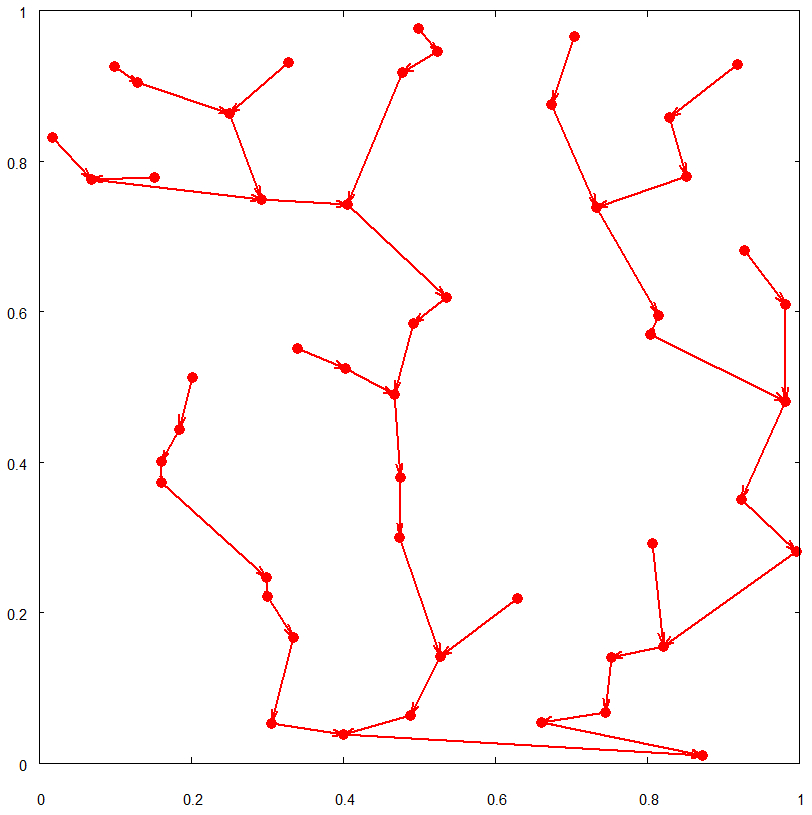
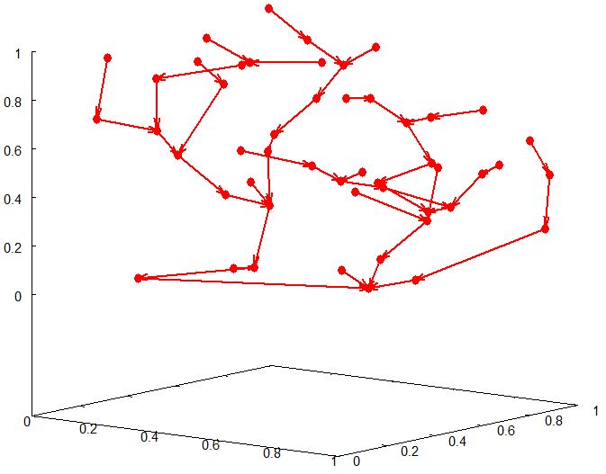
Figure 1: Realizations of the MDST under $\preccurlyeq_{*}$ on 50 simulated uniform random points in $(0,1)^{2}$ (left) and $(0,1)^{3}$ (right).

For $\mathcal{X}\subset\mathbb{R}^{d}$ with ${\rm card}(\mathcal{X})\geq 2$, let $d_{*}({\bf x};\mathcal{X})$ denote the Euclidean distance from a non-minimal ${\bf x}\in\mathcal{X}$ to a directed nearest neighbour ${\bf n}({\bf x};\mathcal{X})$ under $\preccurlyeq_{*}$ and set $d_{*}({\bf m}(\mathcal{X});\mathcal{X})=0$. For $d\in\mathbb{N}$ and $\alpha>0$, define the total power-weighted edge-length of the MDST on $\mathcal{X}$ by

$$\mathcal{L}^{d,\alpha}(\mathcal{X}):=\sum_{{\bf x}\in\mathcal{X}}(d_{*}({\bf x};\mathcal{X}))^{\alpha}=\sum_{{\bf x}\in\mathcal{X}\setminus\{{\bf m}(\mathcal{X})\}}\|{\bf x}-{\bf n}({\bf x};\mathcal{X})\|_{d}^{\alpha},$$

where an empty sum is $0$. In particular, $\mathcal{L}^{d,1}(\mathcal{X})$ is the total Euclidean length of the MDST on $\mathcal{X}$. Also, define the centred version $\tilde{\mathcal{L}}^{d,\alpha}(\mathcal{X}):=\mathcal{L}^{d,\alpha}(\mathcal{X})-{\mathbb{E}}[\mathcal{L}^{d,\alpha}(\mathcal{X})]$.

From now on we will take $\mathcal{X}$ to be a random point set in $(0,1)^{d}$. In particular, we will take a homogeneous Poisson point process $\mathcal{P}_{n}$ of intensity $n$ on $(0,1)^{d}$. Note that in this random setting, each point of $\mathcal{P}_{n}$ almost surely has a unique $x_{d}$-coordinate and at most one directed nearest neighbour under $\preccurlyeq_{*}$, so that $\mathcal{P}_{n}$ has a unique MDST, which is rooted at ${\bf m}(\mathcal{P}_{n})$.

We state and prove all of our main results in the present paper for the Poisson process $\mathcal{P}_{n}$. In all cases, the authors believe that analogous results hold for the binomial point process consisting of $n$ independent uniform random points on $(0,1)^{d}$ instead; it should be possible to use standard de-Poissonization arguments (such as applied in similar circumstances in [22, 23]) to verify this.

In the present paper we are concerned with $d\geq 2$. When $d=1$, $\preccurlyeq_{*}$ coincides with the coordinatewise partial order $\preccurlyeq^{*}$ (and indeed the total order $\leq$ on $\mathbb{R}$) and so our ‘South’ MDST is the same as the ‘South-West’ MDST here. Moreover, $\mathcal{L}^{1,\alpha}(\mathcal{P}_{n})$ is a sum of powers of spacings of uniform points, and it can be studied using standard Dirichlet spacings results (see e.g. [8, 9]). For instance, Darling (see [9], p. 245) essentially gives a central limit theorem for the binomial point process analogue of $\mathcal{L}^{1,\alpha}(\mathcal{P}_{n})$. From now on we fix $d\in\{2,3,\ldots\}$.

Our first result describes the first-order behaviour of $\mathcal{L}^{d,\alpha}(\mathcal{P}_{n})$ as $n\to\infty$. In particular, we have a law of large numbers for $\alpha\in(0,d)$, and also asymptotic results for the expectation when $\alpha\geq d$. In $d=2$, the binomial point process version of Theorem 2.1(i) is contained in the $\phi=\pi$ case of Theorem 5 of [32]. For $d\in\mathbb{N}$, let

$$v_{d}:=\pi^{d/2}\left[\Gamma\left(1+(d/2)\right)\right]^{-1},$$ (1)

the volume of the unit $d$-ball (see e.g. [13] equation (6.50)); here $\Gamma(\cdot)$ denotes the Euler Gamma function.

Theorem 2.1

Suppose $d\in\{2,3,4,\ldots\}$.

• Suppose $\alpha\in(0,d)$. Then as $n\to\infty$,

  $$n^{(\alpha/d)-1}\mathcal{L}^{d,\alpha}(\mathcal{P}_{n})\to 2^{\alpha/d}\Gamma(1+(\alpha/d))v_{d}^{-\alpha/d},\textrm{ in }L^{1}.$$ (2)

• Suppose $\alpha\geq d$. Then there exists $\mu^{\prime}(d,\alpha)\in(0,\infty)$ such that, as $n\to\infty$

  $${\mathbb{E}}[\mathcal{L}^{d,\alpha}(\mathcal{P}_{n})]\to\mu^{\prime}(d,\alpha).$$ (3)

  Moreover, we can express

  $$\mu^{\prime}(d,\alpha)=\mu(d-1,\alpha)+{\bf 1}_{\{\alpha=d\}}2v_{d}^{-1},$$

  where constants $\mu(d-1,\alpha)\in(0,\infty)$ can be characterized in terms of limits of certain on-line nearest-neighbour graphs: $\mu(\cdot,\cdot)$ is as given in Proposition 2.1 of [33]; see (71) below. In particular, for $\alpha\geq 2$

  $$\mu(1,\alpha)=\frac{2}{\alpha(\alpha+1)}\left(1+\frac{2^{-\alpha}}{\alpha-1}\right).$$

One can generalize the statement of Theorem 2.1(i) to more general point processes under certain conditions; see [20, 19] for a general framework.

Our second main result (Theorem 2.2, below) presents convergence in distribution results for $\mathcal{L}^{d,\alpha}(\mathcal{P}_{n})$; the distributional limits contain Gaussian random variables and also random variables defined as distributional limits of certain on-line nearest-neighbour graphs (see Section 3). In general we do not give an explicit description of the latter distributions. However, in the case of $d=2$, the limits in question can be characterized as solutions to distributional fixed-point equations, which we describe at the end of this section.

We now state our main convergence in distribution result. Let $\mathcal{N}(0,s^{2})$ denote the normal distribution with mean zero and variance $s^{2}\geq 0$; included is the degenerate case $\mathcal{N}(0,0)$. By ‘$\stackrel{{\scriptstyle d}}{{\longrightarrow}}$’ we denote convergence in distribution.

Theorem 2.2

Suppose $d\in\{2,3,4,\ldots\}$ and $\alpha>0$. Then there exists a constant $s_{\alpha}^{2}\in[0,\infty)$ such that, for a normal random variable $W_{\alpha}\sim\mathcal{N}(0,s_{\alpha}^{2})$, as $n\to\infty$:

$$n^{(\alpha/d)-(1/2)}\tilde{\cal L}^{d,\alpha}(\mathcal{P}_{n})\stackrel{{\scriptstyle d}}{{\longrightarrow}}W_{\alpha}\leavevmode\nobreak\ \leavevmode\nobreak\ \leavevmode\nobreak\ (0<\alpha<d/2);$$

$$\tilde{\cal L}^{d,d/2}(\mathcal{P}_{n})\stackrel{{\scriptstyle d}}{{\longrightarrow}}W_{d/2}+Q(d-1,d/2);\leavevmode\nobreak\ \leavevmode\nobreak\$$

$$\tilde{\cal L}^{d,\alpha}(\mathcal{P}_{n})\stackrel{{\scriptstyle d}}{{\longrightarrow}}Q(d-1,\alpha)\leavevmode\nobreak\ \leavevmode\nobreak\ \leavevmode\nobreak\ (\alpha>d/2).$$

Here the $Q(d-1,\alpha)$ are mean-zero random variables as given in Lemma 3.2 below and independent of the $W_{\alpha}$; in particular $Q(1,\alpha)=\tilde{G}_{\alpha}$ for $\alpha\geq 1$, where $\tilde{G}_{\alpha}$ has the distribution given by (7) or (2) below.

Remarks. (a) It can be shown that the limiting variance $s_{\alpha}^{2}$ of the normal component in the above limits is strictly positive for $\alpha>0$, using, for example, techniques similar to those in [3] or [27] (see Lemma 6.2 of the extended version of [23] for an example of such a result for a different MDST model).
(b) The normal random variables $W_{\alpha}$ arise from the edges away from the lower boundary of the $d$-cube (see Section 4.2). The variables $Q(d-1,\alpha)$ arise from the edges very close to the boundary, where the MDST is asymptotically close to a $(d-1)$-dimensional on-line nearest-neighbour graph: this is formalized in Section 5 below.
(c) Theorem 2.2 indicates a phase transition in the character of the limit law as $\alpha$ increases. The normal contribution dominates for $\alpha\in(0,d/2)$, while the boundary contribution dominates for $\alpha>d/2$. In the critical case $\alpha=d/2$ (such as the natural case $d=2$ and $\alpha=1$) neither effect dominates and both terms contribute significantly to the asymptotic behaviour. The intuition here is that increasing $\alpha$ increases the relative importance of long edges, such as, typically, those near to the boundary.
(d) As will be demonstrated below (see Lemma 3.2), the random variables $Q(d-1,\alpha)$ can be characterized as distributional limits of certain on-line nearest-neighbour graphs. It is known (see [24]) that the $Q(d-1,\alpha)$ are non-Gaussian for $\alpha>d-1$. When $d=2$ much more is known (see [24]); $Q(1,\alpha)$ can be characterized in terms of a distributional fixed-point equation (see (7) and (2) below). In particular, $Q(1,\alpha)$ is non-Gaussian for $\alpha\geq 1$. The authors suspect that for general $d$, $Q(d-1,\alpha)$ is in fact non-Gaussian for all $\alpha\geq d/2$.

Theorem 2.3 below gives a convergence in distribution result on the length of the longest edge in the MDST on $(\mathcal{P}_{n};\preccurlyeq_{*})$. A similar result (in $d=2$ only) for the longest edge in the ‘South-West’ MDST was given in [22]. Let $\mathcal{L}_{\rm max}^{d}(\mathcal{X})$ denote the length of the longest edge in the MDST (under $\preccurlyeq_{*}$) on point set $\mathcal{X}\subset(0,1)^{d}$:

$$\mathcal{L}_{\rm max}^{d}(\mathcal{X}):=\max_{{\bf x}\in\mathcal{X}}d_{*}({\bf x};\mathcal{X})=\max_{{\bf x}\in\mathcal{X}\setminus\{{\bf m}(\mathcal{X})\}}\|{\bf x}-{\bf n}({\bf x};\mathcal{X})\|_{d}.$$

In the particular case $d=2$, the distributional limit arising in Theorem 2.3 below is expressed in terms of the max-Dickman distribution (named after Dickman’s work [10] on the asymptotic distribution of large prime factors), which can be characterized as the distribution of a random variable $M$ satisfying the fixed-point equation

$$M\stackrel{{\scriptstyle d}}{{=}}\max\{1-U,UM\},$$ (4)

where $U$ is uniform on $(0,1)$ and independent of the $M$ on the right. (Here and subsequently ‘$\stackrel{{\scriptstyle d}}{{=}}$’ denotes equality in distribution.) See [22, 25] and references therein for more information on the max-Dickman distribution; it has appeared in many contexts, and a picture of part of its density function is on the front cover of the second edition of Billingsley’s book [8]. In particular, we note that $M$ can be characterized as the first component of the Poisson–Dirichlet distribution with parameter 1, and ${\mathbb{E}}[M]\approx 0.6243299$ is Dickman’s constant (see [10] p. 9).

Theorem 2.3

Let $d\in\{2,3,\ldots,\}$. There exists a random variable $Q_{\rm max}(d-1)$ such that

$$\mathcal{L}_{\rm max}^{d}(\mathcal{P}_{n})\stackrel{{\scriptstyle d}}{{\longrightarrow}}Q_{\rm max}(d-1),$$

as $n\to\infty$. Moreover, $Q_{\rm max}(d-1)$ is characterized in terms of the ONG (see Theorem 3.1 below); in particular

$$Q_{\rm max}(1)\stackrel{{\scriptstyle d}}{{=}}\max\{UM^{\{1\}},(1-U)M^{\{2\}}\},$$

where $U$, $M^{\{1\}}$ and $M^{\{2\}}$ are independent random variables, $U$ is uniform on $(0,1)$, and $M^{\{1\}}$ and $M^{\{2\}}$ have the max-Dickman distribution as given by (4).

We will derive Theorem 2.3 from a new result on the limiting distribution of the length of the longest edge in the ONG on uniform random points in $(0,1)^{d}$, which is of some independent interest: see Theorem 3.1 below.

As promised, we now give a characterization of the limits $Q(1,\alpha)$, $\alpha\geq 1$, arising in the $d=2$ case of Theorem 2.2. First we define random variables $\tilde{J}_{\alpha}$, $\alpha>1/2$, with ${\mathbb{E}}[\tilde{J}_{\alpha}]=0$ and ${\mathbb{E}}[\tilde{J}_{\alpha}^{2}]<\infty$. Define $\tilde{J}_{1}$ by the fixed-point equation

$$\tilde{J}_{1}\stackrel{{\scriptstyle d}}{{=}}\min\{U,1-U\}+U\tilde{J}_{1}^{\{1\}}+(1-U)\tilde{J}_{1}^{\{2\}}+\frac{1}{2}U\log U+\frac{1}{2}(1-U)\log(1-U),$$ (5)

and for $\alpha\in(1/2,\infty)\setminus\{1\}$, define $\tilde{J}_{\alpha}$ by the fixed-point equation

$$\tilde{J}_{\alpha}\stackrel{{\scriptstyle d}}{{=}}\min\{U,(1-U)\}^{\alpha}+U^{\alpha}\tilde{J}_{\alpha}^{\{1\}}+(1-U)^{\alpha}\tilde{J}_{\alpha}^{\{2\}}+\frac{2^{-\alpha}}{\alpha-1}\left(U^{\alpha}+(1-U)^{\alpha}-1\right).$$ (6)

In each of these two equations (and subsequently), $Y^{\{1\}}$ and $Y^{\{2\}}$ denote independent copies of the random variable $Y$, and $U$ denotes a uniform random variable on $(0,1)$ independent of the other random variables on the right-hand side of the equation.

Note that (5) and (6) define unique square-integrable mean-zero solutions (see e.g. Theorem 3 of Rösler [29]), and hence the distributions of $\tilde{J}_{1}$ and $\tilde{J}_{\alpha}$ are uniquely defined. Moments of $\tilde{J}_{\alpha}$ can be calculated recursively from (5) and (6); see [24] for some information on the first few moments of $\tilde{J}_{1}$, for example. From these moments one can deduce that $\tilde{J}_{\alpha}$, $\alpha>1/2$ is not Gaussian.

Now we can define random variables $\tilde{H}_{\alpha}$, $\tilde{G}_{\alpha}$, again with zero mean and finite variance. Define $\tilde{H}_{1}$ by

$$\tilde{H}_{1}\stackrel{{\scriptstyle d}}{{=}}U\tilde{J}_{1}+(1-U)\tilde{H}_{1}+\frac{U}{2}+\frac{1}{2}U\log U+\frac{1}{2}(1-U)\log(1-U).$$

For $\alpha\in(1/2,\infty)\setminus\{1\}$, define $\tilde{H}_{\alpha}$ by

$$\tilde{H}_{\alpha}\stackrel{{\scriptstyle d}}{{=}}U^{\alpha}\tilde{J}_{\alpha}+(1-U)^{\alpha}\tilde{H}_{\alpha}+U^{\alpha}\left(1+\frac{2^{-\alpha}}{\alpha-1}\right)+((1-U)^{\alpha}-1)\left(\frac{1}{\alpha}+\frac{2^{-\alpha}}{\alpha(\alpha-1)}\right).$$

Define $\tilde{G}_{1}$ by

$$\tilde{G}_{1}\stackrel{{\scriptstyle d}}{{=}}U\tilde{H}_{1}^{\{1\}}+(1-U)\tilde{H}_{1}^{\{2\}}+\frac{1}{4}+\frac{1}{2}U\log U+\frac{1}{2}(1-U)\log(1-U).$$ (7)

Finally, for $\alpha\in(1/2,\infty)\setminus\{1\}$, define $\tilde{G}_{\alpha}$ by

$$\tilde{G}_{\alpha}\stackrel{{\scriptstyle d}}{{=}}{} U^{\alpha}\tilde{H}_{\alpha}^{\{1\}}+(1-U)^{\alpha}\tilde{H}_{\alpha}^{\{2\}}+\left(U^{\alpha}+(1-U)^{\alpha}\right)\left(\frac{1}{\alpha}+\frac{2^{-\alpha}}{\alpha(\alpha-1)}\right)$$

$$-\frac{2}{\alpha(\alpha+1)}\left(1+\frac{2^{-\alpha}}{\alpha-1}\right).$$ (8)

Once again, the distributions of $\tilde{H}_{\alpha}$ and $\tilde{G}_{\alpha}$ are uniquely defined. It is the distribution of $\tilde{G}_{\alpha}$ $(\alpha\geq 1)$ as defined by (7) or (2) that appears in the $d=2$ case of Theorem 2.2.

In the remainder of this paper, we prove Theorems 2.1, 2.2 and 2.3. First, in Section 3 we discuss the ONG, which we use to deal with the boundary effects in the MDST, and prove some new results, which are of some independent interest. In Section 4, we apply general results of Penrose [20, 21] (see also [19]) to prove a law of large numbers and central limit theorem for the total weight of the MDST away from the boundary. In Section 5 we deal with the boundary effects themselves. Then in Section 6 we prove Theorem 2.3. Finally, we complete the proofs of Theorem 2.2 in Section 7 and Theorem 2.1 in Section 8.

Throughout the sequel we make repeated use of Slutsky’s theorem (see, e.g., Durrett [11], p. 72), which says that for sequences of random variables $(X_{n})$, $(Y_{n})$ such that $X_{n}\stackrel{{\scriptstyle d}}{{\longrightarrow}}X$ and $Y_{n}\stackrel{{\scriptstyle P}}{{\longrightarrow}}0$ as $n\to\infty$, we have $X_{n}+Y_{n}\stackrel{{\scriptstyle d}}{{\longrightarrow}}X$ as $n\to\infty$. (Here and subsequently ‘$\stackrel{{\scriptstyle P}}{{\longrightarrow}}$’ denotes convergence in probability.)

3 The on-line nearest-neighbour graph

In this section we describe the on-line nearest-neighbour graph that we use to analyse the boundary effects in the total weight of the MDST under $\preccurlyeq_{*}$. Some of the results that we will require are present in [24] and [33], but we will also need some new results, which we prove in this section.

Let $(\mathbf{Y}_{1},\mathbf{Y}_{2},\ldots)$ be a sequence of vectors in $\mathbb{R}^{d}$, and for $m\in\mathbb{N}$ set $\mathcal{Y}_{m}:=(\mathbf{Y}_{1},\ldots,\mathbf{Y}_{m})$. The on-line nearest-neighbour graph (ONG) on sequence $\mathcal{Y}_{m}$ is constructed by joining each point after the first of $\mathcal{Y}_{m}$ by a directed edge to its (Euclidean) nearest neighbour amongst those points that precede it in the sequence. That is, for $i=2,\ldots,m$ we include the edge $(\mathbf{Y}_{i},\mathbf{Y}_{j})$ where $j\in\{1,\ldots,i-1\}$ is such that

$$\|\mathbf{Y}_{j}-\mathbf{Y}_{i}\|_{d}=\min_{1\leq k<i}\|\mathbf{Y}_{k}-\mathbf{Y}_{i}\|_{d},$$

arbitrarily breaking any ties.

In this way we obtain the ONG on $\mathcal{Y}_{m}$, denoted $\mathrm{ONG}(\mathcal{Y}_{m})$ and which, ignoring directedness of edges, is a tree rooted at $\mathbf{Y}_{1}$. Denote the total power-weighted edge-length with exponent $\alpha>0$ of $\mathrm{ONG}(\mathcal{Y}_{m})$ by $\mathcal{O}^{d,\alpha}(\mathcal{Y}_{m})$, that is

$$\mathcal{O}^{d,\alpha}(\mathcal{Y}_{m}):=\sum_{i=2}^{m}\min_{1\leq j<i}\|\mathbf{Y}_{i}-\mathbf{Y}_{j}\|_{d}^{\alpha};$$

when $\mathcal{Y}_{m}$ is random, we denote the centred version by $\tilde{\cal O}^{d,\alpha}(\mathcal{Y}_{m}):=\mathcal{O}^{d,\alpha}(\mathcal{Y}_{m})-{\mathbb{E}}[\mathcal{O}^{d,\alpha}(\mathcal{Y}_{m})]$.

Our primary interest is the case where $\mathcal{Y}_{m}$ is a sequence of uniform random vectors on the $d$-cube. Let $d\in\mathbb{N}$. Let $(\mathbf{U}_{1},\mathbf{U}_{2},\ldots)$ be a sequence of independent uniform random vectors in $(0,1)^{d}$. For $m\in\mathbb{N}$, set $\mathcal{U}_{m}:=(\mathbf{U}_{1},\ldots,\mathbf{U}_{m})$. We then consider $\mathrm{ONG}(\mathcal{U}_{m})$.

We also consider the ONG defined on a Poisson number of points. Let $(N(t))_{t\geq 0}$ be the counting process of a homogeneous Poisson process of unit rate in $(0,\infty)$, independent of $(\mathbf{U}_{1},\mathbf{U}_{2},\ldots)$. Thus $N(n)$ is a Poisson random variable with mean $n$. With $\mathcal{U}_{m}$ as defined above set $\Pi_{n}=\mathcal{U}_{N(n)}$; we then consider $\mathrm{ONG}(\Pi_{n})$ Note that the points of the sequence $\Pi_{n}$ then constitute a homogeneous Poisson point process of intensity $n$ on $(0,1)^{d}$.

We need the following result, which is contained in Theorem 2.1 of [33].

Lemma 3.1

Suppose $d\in\mathbb{N}$.

• For $\alpha\in(0,d/2)$, there exists a constant $C\in(0,\infty)$ such that for all $n\geq 1$

  $${\mathbb{V}\mathrm{ar}}[\tilde{\cal O}^{d,\alpha}(\Pi_{n})]\leq Cn^{1-(2\alpha/d)}.$$

• For $\alpha=d/2$, there exists a constant $C\in(0,\infty)$ such that for all $n\geq 1$

  $${\mathbb{V}\mathrm{ar}}[\tilde{\cal O}^{d,d/2}(\Pi_{n})]\leq C\log(1+n).$$

The following result is contained in Theorem 2.2 of [33], with Theorem 2.2 of [24] used to deduce the final statement about the $d=1$ case.

Lemma 3.2

Suppose $d\in\mathbb{N}$ and $\alpha>d/2$. Then there exists a mean-zero random variable $Q(d,\alpha)$ such that as $n\to\infty$

$$\tilde{\cal O}^{d,\alpha}(\Pi_{n})\stackrel{{\scriptstyle d}}{{\longrightarrow}}Q(d,\alpha).$$

In particular, $Q(1,\alpha)=\tilde{G}_{\alpha}$ for $\alpha\geq 1$, where $\tilde{G}_{\alpha}$ has distribution given by (7) or (2).

In order to deduce Theorem 2.3, we use the following result on the length of longest edge of the ONG on uniform random points in $(0,1)^{d}$, which adds to the analysis of the ONG given in [6, 18, 24, 32, 33]. For a sequence $\mathcal{Y}_{m}=(\mathbf{Y}_{1},\ldots,\mathbf{Y}_{m})$ of points in $\mathbb{R}^{d}$, let $\mathcal{O}_{\rm max}^{d}(\mathcal{Y}_{m})$ denote the length of the longest edge in the ONG on $\mathcal{Y}_{m}$:

$$\mathcal{O}_{\rm max}^{d}(\mathcal{Y}_{m}):=\max_{2\leq i\leq m}\min_{1\leq j<i}\|\mathbf{Y}_{i}-\mathbf{Y}_{j}\|_{d}.$$

For $d=1$, where $\mathcal{U}_{n}=(U_{1},\ldots,U_{n})$ and $\Pi_{n}=(U_{1},\ldots,U_{N(n)})$ for $U_{1},U_{2},\ldots$ independent uniform random variables on $(0,1)$, we set $\mathcal{U}_{n}^{0}:=(0,U_{1},\ldots,U_{n})$, i.e. $\mathcal{U}_{n}^{0}$ is $\mathcal{U}_{n}$ but with an initial point placed at the origin, and similarly $\Pi_{n}^{0}:=(0,U_{1},\ldots,U_{N(n)})$.

Theorem 3.1

Let $d\in\mathbb{N}$.

• There exists a random variable $Q_{\rm max}(d)$ such that as $n\to\infty$

  $$\mathcal{O}_{\rm max}^{d}(\mathcal{U}_{n})\stackrel{{\scriptstyle d}}{{\longrightarrow}}Q_{\rm max}(d);\leavevmode\nobreak\ \leavevmode\nobreak\ \leavevmode\nobreak\ \mathcal{O}_{\rm max}^{d}(\Pi_{n})\stackrel{{\scriptstyle d}}{{\longrightarrow}}Q_{\rm max}(d).$$

• When $d=1$, we have in particular that

  $$Q_{\rm max}(1)\stackrel{{\scriptstyle d}}{{=}}\max\{UM^{\{1\}},(1-U)M^{\{2\}}\},$$ (9)

  where $U$, $M^{\{1\}}$, $M^{\{2\}}$ are independent, $U$ is uniform on $(0,1)$ and $M^{\{1\}}$, $M^{\{2\}}$ are max-Dickman random variables as given by (4). Also as $n\to\infty$

  $$\mathcal{O}_{\rm max}^{1}(\mathcal{U}^{0}_{n})\stackrel{{\scriptstyle d}}{{\longrightarrow}}M;\leavevmode\nobreak\ \leavevmode\nobreak\ \leavevmode\nobreak\ \mathcal{O}_{\rm max}^{1}(\Pi^{0}_{n})\stackrel{{\scriptstyle d}}{{\longrightarrow}}M,$$ (10)

  where $M$ is a max-Dickman random variable as given by (4).

Proof. First we prove part (i). With probability $1$, for all $n$, $0\leq\mathcal{O}_{\rm max}^{d}(\mathcal{U}_{n})\leq d^{1/2}$ and $\mathcal{O}_{\rm max}^{d}(\mathcal{U}_{n+1})\geq\mathcal{O}_{\rm max}^{d}(\mathcal{U}_{n})$. Hence $\mathcal{O}_{\rm max}^{d}(\mathcal{U}_{n})\to Q_{\rm max}(d)$ a.s., as $n\to\infty$, for some $Q_{\rm max}(d)$. Then by the coupling of $\Pi_{n}$ and $\mathcal{U}_{n}$ and the fact that $N(n)\to\infty$ a.s., we have that with this coupling $\mathcal{O}_{\rm max}^{d}(\Pi_{n})$ converges to the same $Q_{\rm max}$ a.s. and hence in distribution (regardless of the coupling), completing the proof of part (i).

We now prove part (ii) of the theorem, and so take $d=1$. First we prove (10). Again by the coupling of $\Pi_{n}$ and $\mathcal{U}_{n}$, it suffices to prove that $\mathcal{O}_{\rm max}^{1}(\mathcal{U}^{0}_{n})\to M$ a.s. as $n\to\infty$. The following argument is related to the proof of Theorem 2 of [22].

An upper record value in the sequence $X_{1},X_{2},X_{3},\ldots$ is a value $X_{i}$ which exceeds $\max\{X_{1}$, $\ldots$, $X_{i-1}\}$ (the first value $X_{1}$ is also included as a record value). Let $j(1),j(2),\ldots$ be the values of $i\in\mathbb{N}$ such that $U_{i}$ is an upper record in the sequence $(U_{1},U_{2},\ldots)$, arranged in increasing order so that $1=j(1)<j(2)<\cdots$. Let $R_{n}:=\max\{k:j(k)\leq n\}$ be the number of record values in the sequence $\mathcal{U}_{n}=(U_{1},\ldots,U_{n})$.

A record $U_{i}$ has by definition no preceding point in the sequence $\mathcal{U}_{n}$ to its right in the unit interval, and hence (in the ONG on $\mathcal{U}^{0}_{n}$) must be joined to its nearest neighbour to the left amongst those points already present, which is necessarily the previous record value when $i>1$, or $0$ in the case of $U_{1}$. Then each non-record $U_{i}$ lies in an interval between a record value and its nearest neighbour to the left, and hence gives rise to a shorter edge than that from some record value. Thus

$$\mathcal{O}_{\rm max}^{1}(\mathcal{U}_{n}^{0})=\max_{1\leq i\leq R_{n}}\left\{U_{j(i)}-U_{j(i-1)}\right\},$$ (11)

where we set $j(0):=0$ and $U_{0}:=0$. For $i\in\mathbb{N}$ set

$$V_{i}:=\frac{1-U_{j(i)}}{1-U_{j(i-1)}}.$$

It is not hard to see that $V_{1},V_{2},\ldots$ are mutually independent and each is uniformly distributed over $(0,1)$. Therefore, setting

$$M:=\max\{1-V_{1},V_{1}(1-V_{2}),V_{1}V_{2}(1-V_{3}),V_{1}V_{2}V_{3}(1-V_{4}),\ldots\},$$

we obtain

$$M =\max\{1-V_{1},V_{1}\max\{1-V_{2},V_{2}(1-V_{3}),V_{2}V_{3}(1-V_{4}),\ldots\}\}$$

$$=\max\{1-V_{1},V_{1}M^{\prime}\},$$ (12)

where $M^{\prime}:=\max\{1-V_{2},V_{2}(1-V_{3}),V_{2}V_{3}(1-V_{4}),\ldots\}$ has the same distribution as $M$ and is independent of $V_{1}$. Hence $M$ has the max-Dickman distribution as given by (4). Furthermore, with the convention that an empty product is $1$,

$$(1-V_{i})\prod_{k=1}^{i-1}V_{k}=\frac{U_{j(i)}-U_{j(i-1)}}{1-U_{j(i-1)}}\prod_{k=1}^{i-1}\left(\frac{1-U_{j(k)}}{1-U_{j(k-1)}}\right)=U_{j(i)}-U_{j(i-1)},$$ (13)

for $k\in\mathbb{N}$. Also, $R_{n}\to\infty$ almost surely as $n\to\infty$. Hence by (11), (3) and (13),

$$\mathcal{O}_{\rm max}^{1}(\mathcal{U}^{0}_{n})=\max_{1\leq i\leq R_{n}}\left\{(1-V_{i})\prod_{k=1}^{i-1}V_{k}\right\}\to\max_{i\geq 1}\left\{(1-V_{i})\prod_{k=1}^{i-1}V_{k}\right\}=M,$$

where the convergence is almost sure. This proves (10).

To complete the proof of part (ii) of the theorem, we need to prove (9). Conditioning on $U=U_{1}$ and the number of points of $(U_{2},U_{3},\ldots,U_{n})$ that fall in each of the two intervals $(0,U)$, $(U,1)$, we obtain by scaling that

$$\mathcal{O}_{\rm max}^{1}(\mathcal{U}_{n})\stackrel{{\scriptstyle d}}{{=}}\max\{U\mathcal{O}_{\rm max}^{1}(\mathcal{U}^{0}_{L}),(1-U)\mathcal{O}_{\rm max}^{1}(\tilde{\mathcal{U}}^{0}_{n-1-L})\},$$ (14)

where in the right-hand expression $\tilde{\mathcal{U}}^{0}_{m}=(0,\tilde{U}_{1},\tilde{U}_{2},\ldots,\tilde{U}_{m})$, $L\sim{\rm Bin}(n-1,U)$, and $U,U_{1},U_{2},\ldots,\tilde{U}_{1},\tilde{U}_{2},\ldots$ are independent uniform random variables on $(0,1)$. Here $L$ and $n-1-L$ both tend to infinity a.s. as $n\to\infty$, and $\mathcal{O}_{\rm max}^{1}(\mathcal{U}^{0}_{L})$ and $\mathcal{O}_{\rm max}^{1}(\tilde{\mathcal{U}}^{0}_{n-1-L})$ are independent given $L$. Thus by (10) we have that $\mathcal{O}_{\rm max}^{1}(\mathcal{U}^{0}_{L})$ and $\mathcal{O}_{\rm max}^{1}(\tilde{\mathcal{U}}^{0}_{n-1-L})$ converge in distribution to independent copies of the max-Dickman variable $M$. Then (14) and the fact that $Q_{\rm max}(1)$ is the distributional limit of $\mathcal{O}_{\rm max}^{1}(\mathcal{U}_{n})$ yields (9). $\square$

4 Limit theorems away from the boundary

In this section we prove a law of large numbers and central limit theorem for the total power-weighted length of the MDST edges from points that are not too close to the base of the unit $d$-cube. To do this, we employ some general results of Penrose [19, 20, 21].

Recently, notions of stabilizing functionals of point sets have proved to be a useful basis for a general methodology for establishing limit theorems for functionals of random point sets in $\mathbb{R}^{d}$. See for example [18, 20, 21, 26, 27]. To prove the law of large numbers (Lemma 4.1) and central limit theorem (Lemma 4.4) in this section, we make use of the general results on convergence of random measures in geometric probability given in [19, 20, 21]. These two lemmas will then form two of the ingredients for two of our main results, Theorems 2.1 and 2.2.

We use the following notation. Let $d\in\mathbb{N}$. Let $\mathcal{X}\subset\mathbb{R}^{d}$ be finite. For constant $a>0$, and ${\bf y}\in\mathbb{R}^{d}$, let ${\bf y}+a\mathcal{X}$ denote the transformed set $\{{\bf y}+a{\bf x}:{\bf x}\in\mathcal{X}\}$. For ${\bf x}\in\mathbb{R}^{d}$ and $r>0$, let $B({\bf x};r)$ be the closed Euclidean $d$-ball with centre ${\bf x}$ and radius $r$. For bounded measurable $R\subset\mathbb{R}^{d}$ let $|R|$ denote the $d$-dimensional Lebesgue measure of $R$. Write ${\bf 0}$ for the origin of $\mathbb{R}^{d}$.

For $\alpha>0$, define the $[0,\infty)$-valued function on finite non-empty $\mathcal{X}\subset\mathbb{R}^{d}$ and ${\bf x}\in\mathcal{X}$:

$$\xi({\bf x};\mathcal{X}):=d_{*}({\bf x};\mathcal{X})^{\alpha},$$ (15)

and set $\xi({\bf x};\emptyset):=0$ for any ${\bf x}$. Then $\xi$ is translation invariant (that is $\xi({\bf y}+{\bf x};{\bf y}+\mathcal{X})=\xi({\bf x};\mathcal{X})$ for all ${\bf y}\in\mathbb{R}^{d}$, all finite $\mathcal{X}\subset\mathbb{R}^{d}$ and ${\bf x}\in\mathcal{X}$) and homogeneous of order $\alpha$ (that is for any $r>0$, $\xi(r{\bf x};r\mathcal{X})=r^{\alpha}\xi({\bf x};\mathcal{X})$ for all finite $\mathcal{X}\subset\mathbb{R}^{d}$ and ${\bf x}\in\mathcal{X}$). For $\mathcal{X}\subset\mathbb{R}^{d}$ and ${\bf x}\in\mathbb{R}^{d}$, write $\mathcal{X}^{\bf x}$ for $\mathcal{X}\cup\{{\bf x}\}$. If ${\bf x}\notin\mathcal{X}$, we abbreviate notation to $\xi({\bf x};\mathcal{X})=\xi({\bf x};\mathcal{X}^{\bf x})$. The above definitions extend naturally to infinite but locally finite sets $\mathcal{X}$ (as in [20]).

Let

$$\mathcal{L}^{d,\alpha}(\mathcal{X};R):=\sum_{{\bf x}\in\mathcal{X}\cap R}\xi({\bf x};\mathcal{X})$$ (16)

be the translation invariant functional defined on all finite point sets $\mathcal{X}\subset\mathbb{R}^{d}$ and all Borel sets $R\subseteq\mathbb{R}^{d}$ induced by the function $\xi$. Then $\mathcal{L}^{d,\alpha}(\mathcal{X};R)$ is the total power-weighted length of the edges of the MDST on $\mathcal{X}$ originating from points in the region $R$. It is this functional that interests us here. When $\mathcal{X}$ is random, set $\tilde{\mathcal{L}}^{d,\alpha}(\mathcal{X};R):=\mathcal{L}^{d,\alpha}(\mathcal{X};R)-{\mathbb{E}}[\mathcal{L}^{d,\alpha}(\mathcal{X};R)]$. Note that with our previous notation, $\mathcal{L}^{d,\alpha}(\mathcal{X})=\mathcal{L}^{d,\alpha}(\mathcal{X};(0,1)^{d})$ for $\mathcal{X}\subset(0,1)^{d}$.

Fix ${\varepsilon}\in(0,1/d)$ (small). Let $(g_{n})_{n>0}$ be such that $g_{n}\in(0,1)$ and $g_{n}=\Theta(n^{{\varepsilon}-(1/d)})$ as $n\to\infty$, where by $a(n)=\Theta(b(n))$ as $n\to\infty$ we mean

$$0<\liminf_{n\to\infty}\frac{a(n)}{b(n)}\leq\limsup_{n\to\infty}\frac{a(n)}{b(n)}<\infty.$$

Given $g_{n}$, we introduce the family $(\Gamma_{n})_{n\geq 1}$ of Borel subsets of $\mathbb{R}^{d}$ given by

$$\Gamma_{n}:=(0,1)^{d-1}\times(g_{n},1),$$ (17)

i.e. $\Gamma_{n}$ is the unit $d$-cube without a thin strip at the base (in the ${\bf e}_{d}$ sense). Note that the limiting set $\cup_{n\geq 1}\Gamma_{n}=(0,1)^{d}$. Later on, in Section 7, we will make a more specific choice for $g_{n}$. For $n\geq 1$, locally finite $\mathcal{X}\subset\mathbb{R}^{d}$ and ${\bf x}\in\mathcal{X}$ we define the scaled-up version of $\xi$ restricted to $\Gamma_{n}$ by

$$\xi_{n}({\bf x};\mathcal{X}):=\xi(n^{1/d}{\bf x};n^{1/d}\mathcal{X}){\bf 1}_{\Gamma_{n}}({\bf x}).$$

Then, from (16)

$$\mathcal{L}^{d,\alpha}(\mathcal{X};\Gamma_{n})=\sum_{{\bf x}\in\mathcal{X}}\xi({\bf x};\mathcal{X}){\bf 1}_{\Gamma_{n}}({\bf x})=n^{-\alpha/d}\sum_{{\bf x}\in\mathcal{X}}\xi_{n}({\bf x};\mathcal{X}),$$ (18)

using the fact that $\xi$ as given by (15) is homogeneous of order $\alpha$. We employ the following notion of stabilization (see [20, 21]).

Definition 4.1

For any locally finite $\mathcal{X}\subset\mathbb{R}^{d}$ and Borel region $A\subseteq\mathbb{R}^{d}$, define $R_{\xi}({\bf 0};\mathcal{X},A)$ (called the radius of stabilization for $\xi$ at ${\bf 0}$ with respect to $\mathcal{X}$ and $A$) to be the smallest integer $r\geq 0$ such that

$$\xi({\bf 0};(\mathcal{X}\cap B({\bf 0};r))\cup\mathcal{Y})=\xi({\bf 0};\mathcal{X}\cap B({\bf 0};r)),$$

for all finite $\mathcal{Y}\subset A\setminus B({\bf 0};r)$. If no such $r$ exists, set $R_{\xi}({\bf 0};\mathcal{X},A)=\infty$.

When $A$ is all of $\mathbb{R}^{d}$, we write $R_{\xi}({\bf 0};\mathcal{X})$ for $R_{\xi}({\bf 0};\mathcal{X},\mathbb{R}^{d})$.

4.1 Law of large numbers

We will apply a Poisson point process analogue of the law of large numbers Theorem 2.1 of [20]. As mentioned on p. 1130 of [20], such a Poisson-sample result follows by similar arguments to the proofs in [20]; in fact such a result is stated and proved as Theorem 2.1 in [19]. It is this latter result that we will use in this section.

Let $\mathcal{H}_{1}$ denote a homogeneous Poisson point process of unit intensity on $\mathbb{R}^{d}$. Our law of large numbers result for this section is the following.

Lemma 4.1

Suppose $d\in\{2,3,\ldots\}$ and $\alpha>0$. As $n\to\infty$ we have

$$n^{(\alpha/d)-1}\mathcal{L}^{d,\alpha}(\mathcal{P}_{n};\Gamma_{n})\to{\mathbb{E}}[\xi({\bf 0};\mathcal{H}_{1})]=2^{\alpha/d}v_{d}^{-\alpha/d}\Gamma(1+(\alpha/d)),$$ (19)

where the convergence is in $L^{2}$, and $v_{d}$ is given by (1).

The statement (19) will follow from Theorem 2.1 of [19] applied to our functional $\xi$ as defined at (15), using (18). Thus we need to verify the conditions of Theorem 2.1 of [19]: (a) that $R_{\xi}({\bf 0};\mathcal{H}_{1})$ is almost surely finite; and (b) that there exists some $p>2$ such that the following two moments conditions hold:

$$\sup_{n\geq 1;\leavevmode\nobreak\ {\bf x}\in(0,1)^{d}}{\mathbb{E}}[\xi_{n}({\bf x};\mathcal{P}_{n})^{p}]<\infty,\leavevmode\nobreak\ \leavevmode\nobreak\ \textrm{and}$$ (20)

$$\sup_{n\geq 1;\leavevmode\nobreak\ {\bf x},{\bf y}\in(0,1)^{d}}{\mathbb{E}}[\xi_{n}({\bf x};\mathcal{P}^{\bf y}_{n})^{p}]<\infty.$$ (21)

The next two lemmas take care of this.

Lemma 4.2

For $\xi$ given by (15), the radius of stabilization $R_{\xi}({\bf 0};\mathcal{H}_{1})$ as defined in Definition 4.1 is almost surely finite.

Proof. Let $R=d_{*}({\bf 0};\mathcal{H}_{1})$. Then $R$ is finite almost surely. For any $\ell>R$ we have that $\xi({\bf 0};(\mathcal{H}_{1}\cap B({\bf 0};\ell))\cup{\cal Y})=R^{\alpha}$, for any finite ${\cal Y}\subset\mathbb{R}^{d}\setminus B({\bf 0};\ell)$. Thus taking $R_{\xi}({\bf 0};\mathcal{H}_{1})$ to be the smallest integer greater than $R$, $R_{\xi}({\bf 0};\mathcal{H}_{1})$ is almost surely finite. $\square$

Lemma 4.3

Suppose $d\in\{2,3,\ldots\}$ and $\alpha>0$. Then for $(\Gamma_{n})_{n\geq 1}$ as given at (17) and $\xi$ as given by (15) the moments conditions (20) and (21) hold for any $p>0$.

Proof. We have from the definition of $\xi_{n}$ and (15) that

$$\sup_{{\bf x}\in(0,1)^{d}}{\mathbb{E}}[\xi_{n}({\bf x};\mathcal{P}_{n})^{p}]=\sup_{{\bf x}\in\Gamma_{n}}{\mathbb{E}}[\xi(n^{1/d}{\bf x};n^{1/d}\mathcal{P}_{n})^{p}]=\sup_{{\bf x}\in\Gamma_{n}}{\mathbb{E}}[d_{*}(n^{1/d}{\bf x};n^{1/d}\mathcal{P}_{n})^{\alpha p}].$$ (22)

For $d\in\{2,3,\ldots\}$, ${\bf x}\in\Gamma_{n}$ and $r>0$, define the region in the scaled-up space $(0,n^{1/d})^{d}$

$$A^{d}_{n}({\bf x},r):=B(n^{1/d}{\bf x};r)\cap(0,n^{1/d})^{d}\cap\{{\bf y}\in\mathbb{R}^{d}:{\bf y}\preccurlyeq_{*}n^{1/d}{\bf x}\}.$$ (23)

For ${\bf x}\in\Gamma_{n}$, define the variables $\zeta_{n}^{(1)}({\bf x}):=d_{*}(n^{1/d}{\bf x};n^{1/d}\mathcal{P}_{n}){\bf 1}_{\{d_{*}({\bf x};\mathcal{P}_{n})\leq g_{n}\}}$ and $\zeta_{n}^{(2)}({\bf x}):=d_{*}(n^{1/d}{\bf x};n^{1/d}\mathcal{P}_{n}){\bf 1}_{\{d_{*}({\bf x};\mathcal{P}_{n})>g_{n}\}}$. For $t\geq 0$,

$${\mathbb{P}}(\zeta_{n}^{(1)}({\bf x})>t)={\mathbb{P}}(\{d_{*}(n^{1/d}{\bf x};n^{1/d}\mathcal{P}_{n})>t\}\cap\{d_{*}(n^{1/d}{\bf x};n^{1/d}\mathcal{P}_{n})\leq n^{1/d}g_{n}\}).$$

This probability is clearly zero unless $t<n^{1/d}g_{n}$, in which case, by the definition of $\Gamma_{n}$ the region $A_{n}^{d}({\bf x},t)$ does not touch the hyperplane $\{x_{d}=0\}$, so that $|A_{n}^{d}({\bf x},t)|\geq 2^{-d}v_{d}t^{d}$, where $v_{d}$ is the volume of the unit $d$-ball given by (1). Hence for all $t\geq 0$,

$${\mathbb{P}}(\zeta_{n}^{(1)}({\bf x})>t)\leq\exp(-2^{-d}v_{d}t^{d})$$

so that for all $n$ and all ${\bf x}\in\Gamma_{n}$, $\zeta_{n}^{(1)}({\bf x})$ is stochastically dominated by a variable with cumulative distribution function $F(t)=1-\exp(-2^{-d}v_{d}t^{d})$, $t\geq 0$. Such a variable has finite $(\alpha p)$-th moment.

Also, for all $n$ and all ${\bf x}\in\Gamma_{n}$, the random variable $\zeta_{n}^{(2)}({\bf x})$ is bounded by the random variable $d^{1/2}n^{1/d}{\bf 1}_{\{d_{*}(n^{1/d}{\bf x};n^{1/d}\mathcal{P}_{n})>n^{1/d}g_{n}\}}$, so that

$${\mathbb{E}}[(\zeta_{n}^{(2)}({\bf x}))^{\alpha p}]\leq d^{\alpha p/2}n^{\alpha p/d}{\mathbb{P}}(d_{*}(n^{1/d}{\bf x};n^{1/d}\mathcal{P}_{n})>n^{1/d}g_{n})$$

$$\leq d^{\alpha p/2}n^{\alpha p/d}\exp(-|A_{n}^{d}({\bf x},n^{1/d}g_{n})|)\leq d^{\alpha p/2}n^{\alpha p/d}\exp(-2^{-d}v_{d}(n^{1/d}g_{n})^{d})$$

and since $n^{1/d}g_{n}=\Theta(n^{\varepsilon})$, this upper bound is bounded in $n$. Thus the $(\alpha p)$-th moment of $\zeta_{n}^{(2)}({\bf x})$ is bounded uniformly over all $n$ and all ${\bf x}\in\Gamma_{n}$. Combined with the earlier uniform moment bound for $\zeta_{n}^{(1)}({\bf x})$ and (22), this yields (20).

For (21), note that for any ${\bf x}\in\Gamma_{n},{\bf y}\in(0,1)^{d}$

$$\xi_{n}({\bf x};\mathcal{P}_{n}^{\bf y})=d_{*}(n^{1/d}{\bf x};n^{1/d}(\mathcal{P}_{n}\cup\{{\bf y}\}))^{\alpha}\leq d_{*}(n^{1/d}{\bf x};n^{1/d}\mathcal{P}_{n})^{\alpha}+{\bf 1}_{\{\mathcal{P}_{n}\subset\Gamma_{n}\}}n^{\alpha/d}d^{\alpha/2}.$$

Moreover, $\xi_{n}({\bf x};\mathcal{P}_{n}^{\bf y})$ is zero for ${\bf x}\in(0,1)^{d}\setminus\Gamma_{n}$. Thus

$$\sup_{{\bf x},{\bf y}\in(0,1)^{d}}{\mathbb{E}}\left[\xi_{n}({\bf x};\mathcal{P}_{n}^{\bf y})^{p}\right]\leq\sup_{{\bf x}\in(0,1)^{d}}{\mathbb{E}}\left[\xi_{n}({\bf x};\mathcal{P}_{n})^{p}\right]+{\mathbb{P}}(\mathcal{P}_{n}\subset\Gamma_{n})n^{\alpha p/d}d^{\alpha p/2},$$

so that (20) implies (21) since ${\mathbb{P}}(\mathcal{P}_{n}\subset\Gamma_{n})=\exp(-ng_{n})$. $\square$

Proof of Lemma 4.1. From Theorem 2.1 of [19], with (18) and Lemmas 4.2 and 4.3, we obtain the convergence statement in (19). It remains to prove the final equality (19). We have, for $s\geq 0$

$${\mathbb{P}}\left(\xi({\bf 0};\mathcal{H}_{1})>s\right)={\mathbb{P}}\left(\mathcal{H}_{1}\cap\{{\bf x}\in\mathbb{R}^{d}:{\bf x}\preccurlyeq_{*}{\bf 0}\}\cap B({\bf 0};s^{1/\alpha})=\emptyset\right)=\exp{(-(v_{d}/2)s^{d/\alpha})}.$$

Hence,

$${\mathbb{E}}\left[\xi({\bf 0};\mathcal{H}_{1})\right]=\int_{0}^{\infty}{\mathbb{P}}\left(\xi({\bf 0};\mathcal{H}_{1})>s\right)\mathrm{d}s=\int_{0}^{\infty}\exp(-(v_{d}/2)s^{d/\alpha})\mathrm{d}s,$$

which by the change of variables $y=(v_{d}/2)s^{d/\alpha}$ is the same as

$$\frac{\alpha}{d}2^{\alpha/d}v_{d}^{-\alpha/d}\int_{0}^{\infty}y^{(\alpha/d)-1}\exp(-y)\mathrm{d}y=\frac{\alpha}{d}2^{\alpha/d}v_{d}^{-\alpha/d}\Gamma(\alpha/d),$$

by Euler’s Gamma integral (see e.g. 6.1.1 in [1]). The desired equality now follows from the functional relation $x\Gamma(x)=\Gamma(1+x)$ (see 6.1.15 in [1]). $\square$

4.2 Central limit theorem

We again consider $\mathcal{L}^{d,\alpha}(\mathcal{P}_{n};\Gamma_{n})$ as given by (18). In this section we aim to prove a central limit theorem complementing the law of large numbers of Section 4.1. This time, we will apply Theorems 2.1 and 2.2 of [21] to give the following result.

Lemma 4.4

Let $d\in\{2,3,\ldots\}$ and $\alpha>0$. There exists a constant $s_{\alpha}\in[0,\infty)$, not depending on the choice of ${\varepsilon}$ or the sequence $g_{n}$, such that, as $n\to\infty$,

$$\lim_{n\to\infty}\left(n^{(2\alpha/d)-1}{\mathbb{V}\mathrm{ar}}\left[\mathcal{L}^{d,\alpha}(\mathcal{P}_{n};\Gamma_{n})\right]\right)=\lim_{n\to\infty}\left(n^{-1}{\mathbb{V}\mathrm{ar}}\left[\sum_{{\bf x}\in\mathcal{P}_{n}}\xi_{n}({\bf x};\mathcal{P}_{n})\right]\right)=s_{\alpha}^{2},$$

and

$$n^{(\alpha/d)-(1/2)}\tilde{\mathcal{L}}^{d,\alpha}(\mathcal{P}_{n};\Gamma_{n})\stackrel{{\scriptstyle d}}{{\longrightarrow}}\mathcal{N}(0,s_{\alpha}^{2}).$$

Proof. In order to prove this lemma, we need to verify the conditions of Theorems 2.1 and 2.2 of [21] (see also Theorem 2.2 and 2.3 of [19]) for our function $\xi$ as given by (15). In addition to the moments conditions (20), (21) (as shown to hold in Lemma 4.3), we need to demonstrate the following additional stabilization conditions:

$${\mathbb{P}}(R_{\xi}({\bf 0};\mathcal{H}_{1}^{\bf z})<\infty)=1,$$ (24)

for all ${\bf z}\in\mathbb{R}^{d}$; and

$$\limsup_{s\to\infty}s^{-1}\log\left(\sup_{n\geq 1;\leavevmode\nobreak\ {\bf x}\in\Gamma_{n}}{\mathbb{P}}(R_{\xi}(n^{1/d}{\bf x};n^{1/d}\mathcal{P}_{n},n^{1/d}(0,1)^{d})>s)\right)<0.$$ (25)

Condition (24) requires that the radius of stabilization is almost surely finite on the addition of an arbitrary extra point to $\mathcal{H}_{1}$, and condition (25) requires exponential decay of the tail of the radius of stabilization.

Given Lemma 4.2, (24) is clear, since with probability $1$ the addition of any extra point ${\bf z}\in\mathbb{R}^{d}$ to $\mathcal{H}_{1}$ can only decrease the radius of stabilization at ${\bf 0}$.

We need to prove (25). Let $|A^{d}_{n}({\bf x},r)|$ be defined by (23), and for ${\bf z}=(z_{1},z_{2},\ldots,z_{d})\in n^{1/d}\Gamma_{n}$, let $m({\bf z}):=z_{d}$, the last component of ${\bf z}$. For $d\geq 2$, we claim that there are finite constants $C_{d}>0$ and $n_{0}\geq 1$ such that

$$|A^{d}_{n}({\bf x},r)|\geq C_{d}r^{d-1}\leavevmode\nobreak\ \textrm{if}\leavevmode\nobreak\ r\in(1,d^{1/2}n^{1/d}],$$ (26)

for all $n\in\mathbb{N}$ with $n\geq n_{0}$, and any ${\bf x}\in\Gamma_{n}$.

We verify the claim (26). Take $n_{0}$ such that for all $n\geq n_{0}$ we have $n^{1/d}g_{n}\geq 1$. Then for $n\geq n_{0}$, suppose $r\in(1,d^{1/2}n^{1/d}]$. For a lower bound on the volume of $A^{d}_{n}({\bf x},r)$, consider ${\bf x}=(0,0,\ldots,0,m({\bf x}))$, the ‘worst case’. Let $h_{\bf x}$ denote the hyperplane $\{{\bf y}\in n^{1/d}\Gamma_{n}:m({\bf y})=m(n^{1/d}{\bf x})\}$. Let $r^{\prime}:=d^{-1/2}r$, so $r^{\prime}\leq n^{1/d}$. Then let ${\bf w}_{1},{\bf w}_{2},\ldots,{\bf w}_{d-1}$ denote the $d-1$ points of $h_{\bf x}$ $(r^{\prime},0,0,\ldots,0,m(n^{1/d}{\bf x}))$, $(0,r^{\prime},0,\ldots,0,m(n^{1/d}{\bf x}))$, …$(0,0,\ldots,0,r^{\prime},m(n^{1/d}{\bf x}))$, and let ${\bf w}_{0}$ denote the point $(0,0,\ldots,0,m(n^{1/d}{\bf x})-1)$. Then since ${\bf x}\in\Gamma_{n}$, the $d$-dimensional ‘right pyramid’ defined by vertices ${\bf w}_{0},n^{1/d}{\bf x},{\bf w}_{1},\ldots,{\bf w}_{d-1}$ is contained within both $(0,n^{1/d})^{d}$ and the half-ball $B(n^{1/d}{\bf x};r)\cap\{{\bf y}\in\mathbb{R}^{d}:{\bf y}\preccurlyeq_{*}n^{1/d}{\bf x}\}$. The volume of this ‘pyramid’ is $d!^{-1}(r^{\prime})^{d-1}$. This gives a lower bound for $|A^{d}_{n}({\bf x},r)|$, and (26) holds as claimed.

To prove (25), note that $n^{1/d}\mathcal{P}_{n}$ is a homogeneous Poisson point process of unit intensity on $(0,n^{1/d})^{d}$. Then for $s>1$, arguing as in the proof of Lemma 4.2 yields

$${\mathbb{P}}\left(R_{\xi}(n^{1/d}{\bf x};n^{1/d}\mathcal{P}_{n},n^{1/d}(0,1)^{d})>s\right)\leq{\mathbb{P}}\left(d_{*}(n^{1/d}{\bf x};n^{1/d}\mathcal{P}_{n})>s-1\right)$$

$$\leq\exp\left(-\left|A_{n}^{d}({\bf x},s-1)\right|\right).$$

So by (26), for $n\geq n_{0}$ and $2<s\leq d^{1/2}n^{1/d}+1$, we obtain,

$$\sup_{{\bf x}\in\Gamma_{n}}{\mathbb{P}}\left(R_{\xi}(n^{1/d}{\bf x};n^{1/d}\mathcal{P}_{n},n^{1/d}(0,1)^{d})>s\right)\leq\exp\left(-C_{d}(s-1)^{d-1}\right).$$

Also, this probability is zero for $s>d^{1/2}n^{1/d}+1$. Thus for any $s>d^{1/2}n_{0}^{1/d}+1$,

$$\sup_{n\geq 1;\leavevmode\nobreak\ {\bf x}\in\Gamma_{n}}{\mathbb{P}}\left(R_{\xi}(n^{1/d}{\bf x};n^{1/d}\mathcal{P}_{n},n^{1/d}(0,1)^{d})>s\right) \leq\exp\left(-C_{d}(s-1)^{d-1}\right),$$

and (25) follows. $\square$

5 Boundary effects in the MDST

In this section, we consider the contribution to the total power-weighted length of the MDST under $\preccurlyeq_{*}$ due to boundary effects near the ‘bottom face’ of the $d$-cube. Here the possibility of long edges leads to rather special behaviour. We shall see that the on-line nearest-neighbour graph, as described in Section 3, will be a useful tool here.

Fix ${\varepsilon}>0$ small. Let $(t_{n})_{n>0}$ be such that $t_{n}\in(0,1)$ and $t_{n}=\Theta(n^{-(1/2)-{\varepsilon}})$ as $n\to\infty$ (we make a specific choice for $t_{n}$ in Section 7). Let $B_{n}$ denote the boundary region $(0,1)^{d-1}\times(0,t_{n}]$, i.e. we look in a thin slice at the base (in the sense of $\preccurlyeq_{*}$) of the unit $d$-cube. Recall from (16) that $\mathcal{L}^{d,\alpha}(\mathcal{X};R)$ denotes the contribution to the total weight of the MDST on $\mathcal{X}$ from those points of $\mathcal{X}\cap R$, and $\tilde{\mathcal{L}}^{d,\alpha}(\mathcal{X};R):=\mathcal{L}^{d,\alpha}(\mathcal{X};R)-{\mathbb{E}}[\mathcal{L}^{d,\alpha}(\mathcal{X};R)]$. Also recall that $\mathcal{P}_{n}$ denotes a homogeneous Poisson point process of intensity $n$ on $(0,1)^{d}$. Our main result of this section is the following.

Theorem 5.1

Suppose $d\in\{2,3,\ldots\}$. Let ${\varepsilon}>0$ and $t_{n}=\Theta(n^{-(1/2)-{\varepsilon}})$ specify $B_{n}$.

• Suppose $\alpha\geq d/2$. With $Q(d-1,\alpha)$ as in Lemma 3.2, we have that as $n\to\infty$

  $$\tilde{\mathcal{L}}^{d,\alpha}(\mathcal{P}_{n};B_{n})\stackrel{{\scriptstyle d}}{{\longrightarrow}}Q(d-1,\alpha).$$ (27)

• Suppose $\alpha\in(0,d/2)$. As $n\to\infty$,

  $$n^{(\alpha/d)-(1/2)}\tilde{\mathcal{L}}^{d,\alpha}(\mathcal{P}_{n};B_{n})\stackrel{{\scriptstyle P}}{{\longrightarrow}}0.$$ (28)

The idea behind the proof of Theorem 5.1 is to show that the MDST under $\preccurlyeq_{*}$ near to the boundary is close to an ONG defined on a sequence of uniform random vectors in $(0,1)^{d-1}$ coupled to the points of the MDST in $B_{n}$. To do this, we produce an explicit sequence of random variables on which we construct the ONG coupled to $\mathcal{P}_{n}$ on which the MDST is constructed.

Define the point process

$$\mathcal{W}_{n}:=\mathcal{P}_{n}\cap B_{n}.$$ (29)

Let $\beta_{n}:={\rm card}(\mathcal{W}_{n})$. List $\mathcal{W}_{n}$ in order of increasing $x_{d}$-coordinate as $\mathbf{U}_{i}$, $i=1,2,\ldots,\beta_{n}$. In coordinates, set $\mathbf{U}_{i}=(U_{i}^{1},U_{i}^{2},\ldots,U_{i}^{d})$ for each $i$. Let $\mathbf{V}_{i}=(U_{i}^{1},\ldots,U^{d-1}_{i})\in(0,1)^{d-1}$ be the projection of $\mathbf{U}_{i}$ down (in the ${\bf e}_{d}$ sense) onto the base of the unit $d$-cube. Set

$${\cal V}_{n}:=(\mathbf{V}_{1},\ldots,\mathbf{V}_{\beta_{n}}).$$ (30)

Then ${\cal V}_{n}$ is a sequence of uniform random vectors in $(0,1)^{d-1}$ (the base of the unit $d$-cube), on which we may construct the ONG as appropriate. Note that the points of ${\cal V}_{n}$ in fact constitute a homogeneous Poisson point process of intensity $nt_{n}=\Theta(n^{(1/2)-{\varepsilon}})$ on $(0,1)^{d-1}$ (this follows from the Mapping Theorem, see [15]). With the ONG weight functional $\mathcal{O}^{d,\alpha}(\cdot)$ defined in Section 3, the ONG weight $\mathcal{O}^{d-1,\alpha}({\cal V}_{n})$ is coupled in a natural way to $\mathcal{L}^{d,\alpha}(\mathcal{W}_{n})=\mathcal{L}^{d,\alpha}(\mathcal{P}_{n};B_{n})$.

Our first step towards Theorem 5.1 is the following result, which shows that, near the boundary, the MDST is close to the coupled ONG.

Lemma 5.1

Suppose $d\in\{2,3,\ldots\}$. Let ${\varepsilon}>0$ and $t_{n}=\Theta(n^{-(1/2)-{\varepsilon}})$ specify $B_{n}$. Let $\mathcal{W}_{n},{\cal V}_{n}$ be as defined at (29), (30) respectively. For $\alpha\geq 1$, as $n\to\infty$,

$$\mathcal{L}^{d,\alpha}(\mathcal{W}_{n})-\mathcal{O}^{d-1,\alpha}({\cal V}_{n})\to 0,\textrm{ in }L^{1},$$ (31)

and, for $\alpha\in(0,1)$, as $n\to\infty$,

$${\mathbb{E}}\left|\mathcal{L}^{d,\alpha}(\mathcal{W}_{n})-\mathcal{O}^{d-1,\alpha}({\cal V}_{n})\right|=O\left(n^{(1/2)-{\varepsilon}-\alpha((1/2)+{\varepsilon})}\right).$$ (32)

Proof. We construct the MDST on the set of points $\mathcal{W}_{n}$, and construct the ONG on the projections down onto $(0,1)^{d-1}$, ${\cal V}_{n}$. With a slight abuse of notation, consider the points $\mathbf{U}_{i}=(\mathbf{V}_{i},U^{d}_{i})$, $i=1,\ldots,\beta_{n}$.

Note that by construction of the MDST on $\preccurlyeq_{*}$ and the ONG, and our choice of ordering of points, we have that $\mathbf{U}_{j}\preccurlyeq_{*}\mathbf{U}_{i}$ if and only if $j\leq i$. Thus either an edge exists from $\mathbf{U}_{i}$ in the MDST and also from $\mathbf{V}_{i}$ in the ONG, or from neither. For the difference between the total weights of the two models, it suffices to consider the case in which both edges exist. Then $\mathbf{V}_{i}$ is joined to a point $\mathbf{V}_{D(i)}$, $D(i)<i$ in the ONG, and $\mathbf{U}_{i}$ to a point $\mathbf{U}_{J(i)}$ in the MDST; we do not necessarily have $J(i)=D(i)$. Since $J(i)<i$ by construction of the MDST on $\preccurlyeq_{*}$ and the ordering of our points, we have that $\mathbf{V}_{J(i)}$ was an admissible candidate to be the point that $\mathbf{V}_{i}$ joins to in the ONG. Therefore, we have that $\|\mathbf{V}_{i}-\mathbf{V}_{D(i)}\|_{d-1}\leq\|\mathbf{V}_{i}-\mathbf{V}_{J(i)}\|_{d-1}$. It then follows that

$$\|(\mathbf{V}_{i},U_{i}^{d})-(\mathbf{V}_{J(i)},U^{d}_{J(i)})\|_{d}^{\alpha}\geq\|\mathbf{V}_{i}-\mathbf{V}_{J(i)}\|_{d-1}^{\alpha}\geq\|\mathbf{V}_{i}-\mathbf{V}_{D(i)}\|_{d-1}^{\alpha},$$ (33)

and so we have that, for all $\alpha>0$,

$$\mathcal{O}^{d-1,\alpha}({\cal V}_{n})\leq\mathcal{L}^{d,\alpha}(\mathcal{W}_{n}).$$ (34)

Also, by construction of the ONG and our ordering on points, we see $(\mathbf{V}_{D(i)},U^{d}_{D(i)})\preccurlyeq_{*}(\mathbf{V}_{i},U^{d}_{i})$. So by the construction of the MDST, we have that

$$\|(\mathbf{V}_{i},U^{d}_{i})-(\mathbf{V}_{J(i)},U^{d}_{J(i)})\|_{d}\leq\|(\mathbf{V}_{i},U^{d}_{i})-(\mathbf{V}_{D(i)},U^{d}_{D(i)})\|_{d}.$$ (35)

If $({\bf x},y)\in(0,1)^{d-1}\times(0,1)$ then $\|({\bf x},y)\|_{d}\leq\|{\bf x}\|_{d-1}+y$, and by the Mean Value Theorem for the function $t\mapsto t^{\alpha}$, for $\alpha\geq 1$,

$$\|({\bf x},y)\|_{d}^{\alpha}-\|{\bf x}\|_{d-1}^{\alpha}\leq(\|{\bf x}\|_{d-1}+y)^{\alpha}-\|{\bf x}\|_{d-1}^{\alpha}\leq\alpha((d-1)^{1/2}+1)^{\alpha-1}y\leavevmode\nobreak\ \leavevmode\nobreak\ \leavevmode\nobreak\ (\alpha\geq 1).$$

So we have that, for $d\geq 2$ and $\alpha\geq 1$, there is a finite positive $C$ such that, a.s.,

$$\|(\mathbf{V}_{i},U^{d}_{i})-(\mathbf{V}_{D(i)},U^{d}_{D(i)})\|_{d}^{\alpha}-\|\mathbf{V}_{i}-\mathbf{V}_{D(i)}\|_{d-1}^{\alpha}\leq C(U^{d}_{i}-U^{d}_{D(i)}).$$ (36)

Then (35) and (36) yield, for $\alpha\geq 1$, a.s.,

$$\|(\mathbf{V}_{i},U^{d}_{i})-(\mathbf{V}_{J(i)},U^{d}_{J(i)})\|_{d}^{\alpha}-\|\mathbf{V}_{i}-\mathbf{V}_{D(i)}\|_{d-1}^{\alpha}\leq C(U^{d}_{i}-U^{d}_{D(i)})\leq Ct_{n},$$ (37)

which implies that there exist $C,C^{\prime}\in(0,\infty)$ such that for all $n\geq 1$

$$\mathcal{L}^{d,\alpha}(\mathcal{W}_{n})-\mathcal{O}^{d-1,\alpha}({\cal V}_{n})\leq C\beta_{n}t_{n}\leq C^{\prime}\beta_{n}n^{-(1/2)-{\varepsilon}}.$$ (38)

Combining (34) and (38) we have that, for $\alpha\geq 1$, some $C\in(0,\infty)$ and all $n\geq 1$, a.s.,

$$\left|\mathcal{L}^{d,\alpha}(\mathcal{W}_{n})-\mathcal{O}^{d-1,\alpha}({\cal V}_{n})\right|\leq C\beta_{n}n^{-(1/2)-{\varepsilon}}.$$

Taking expectations, using the facts that $\beta_{n}$ is Poisson with mean $nt_{n}=\Theta(n^{(1/2)-{\varepsilon}})$ and ${\varepsilon}>0$, we obtain (31).

Now we consider the case $\alpha\in(0,1)$. By the concavity of the function $t\mapsto t^{\alpha}$ for $\alpha\in(0,1)$, we have for $({\bf x},y)\in(0,1)^{d-1}\times(0,1)$ that

$$\|({\bf x},y)\|_{d}^{\alpha}-\|{\bf x}\|_{d-1}^{\alpha}\leq(\|{\bf x}\|_{d-1}+y)^{\alpha}-\|{\bf x}\|_{d-1}^{\alpha}\leq y^{\alpha}\leavevmode\nobreak\ \leavevmode\nobreak\ \leavevmode\nobreak\ (0<\alpha<1).$$

Then, by a similar argument to the $\alpha\geq 1$ case, we obtain

$$\left|\mathcal{L}^{d,\alpha}(\mathcal{W}_{n})-\mathcal{O}^{d-1,\alpha}({\cal V}_{n})\right|\leq C\beta_{n}n^{-\alpha((1/2)+{\varepsilon})},$$

so taking expectations yields (32). $\square$

Lemma 5.2

Suppose $d\in\{2,3,\ldots\}$ and $\alpha\geq d/2$. Let $\mathcal{W}_{n}$ be as defined at (29) and suppose that $Q(d-1,\alpha)$ is the mean-zero random variable given in Lemma 3.2. Then as $n\to\infty$

$$\tilde{\mathcal{L}}^{d,\alpha}(\mathcal{W}_{n})\stackrel{{\scriptstyle d}}{{\longrightarrow}}Q(d-1,\alpha).$$ (39)

In particular, $Q(1,\alpha)=\tilde{G}_{\alpha}$ for $\alpha\geq 1$, where $\tilde{G}_{\alpha}$ has the distribution given by (7) or (2).

Proof. For $\alpha\geq d/2\geq 1$, it follows from (31) that as $n\to\infty$

$$\tilde{\mathcal{L}}^{d,\alpha}(\mathcal{W}_{n})-\tilde{\mathcal{O}}^{d-1,\alpha}({\cal V}_{n})\stackrel{{\scriptstyle P}}{{\longrightarrow}}0.$$ (40)

Also, since ${\cal V}_{n}$ is a homogeneous Poisson point process of intensity $nt_{n}=\Theta(n^{(1/2)-{\varepsilon}})$ on $(0,1)^{d-1}$, and $\alpha\geq d/2>(d-1)/2$, we have from Lemma 3.2 that as $n\to\infty$

$$\tilde{\mathcal{O}}^{d-1,\alpha}({\cal V}_{n})\stackrel{{\scriptstyle d}}{{\longrightarrow}}Q(d-1,\alpha).$$ (41)

Thus (40), (41) and Slutsky’s theorem complete the proof of (39). $\square$

Proof of Theorem 5.1. For $\alpha\geq d/2$, (27) follows from (39). Now suppose $\alpha\in(0,d/2)$. First suppose that $\alpha<1$. Then (32) implies that for $\alpha\in(0,1)$

$${\mathbb{E}}\left[n^{(\alpha/d)-(1/2)}\left|\mathcal{L}^{d,\alpha}(\mathcal{P}_{n};B_{n})-\mathcal{O}^{d-1,\alpha}({\cal V}_{n})\right|\right]=O(n^{\alpha((1/d)-(1/2))-{\varepsilon}(1+\alpha)})\to 0,$$

since $d\geq 2$ and ${\varepsilon}>0$. So for $\alpha\in(0,1)$ we have

$$n^{(\alpha/d)-(1/2)}\left(\tilde{\mathcal{L}}^{d,\alpha}(\mathcal{P}_{n};B_{n})-\tilde{\cal O}^{d-1,\alpha}({\cal V}_{n})\right)\to 0,\textrm{ in }L^{1},$$ (42)

as $n\to\infty$. Also, (31) implies that (42) also holds for $\alpha\in[1,d/2)$ when $d\geq 3$. Thus (42) holds for all $\alpha\in(0,d/2)$. Recall that ${\cal V}_{n}$ is a homogeneous Poisson point process in $(0,1)^{d-1}$ with intensity $nt_{n}=\Theta(n^{(1/2)-{\varepsilon}})$. If $\alpha\leq(d-1)/2$, then by Lemma 3.1(i) and (ii) we have that for some $C\in(0,\infty)$

$${\mathbb{V}\mathrm{ar}}\left[n^{(\alpha/d)-(1/2)}\tilde{\cal O}^{d-1,\alpha}({\cal V}_{n})\right]\leq Cn^{(2\alpha/d)-1}(n^{(1/2)-{\varepsilon}})^{1-(2\alpha/(d-1))}\log n$$

$$\leq Cn^{\alpha((2/d)-1/(d-1))-(1/2)}\log n\leq Cn^{-1/d}\log n\to 0,$$

as $n\to\infty$. If $\alpha\in((d-1)/2,d/2)$, then by Lemma 3.2, as $n\to\infty$

$$n^{(\alpha/d)-(1/2)}\tilde{\cal O}^{d-1,\alpha}({\cal V}_{n})\stackrel{{\scriptstyle P}}{{\longrightarrow}}0.$$

So by Slutsky’s theorem with (42) we obtain (28). $\square$

6 Proof of Theorem 2.3

In this section we are interested in the longest edge in the MDST under $\preccurlyeq_{*}$ on $\mathcal{P}_{n}\subset(0,1)^{d}$. The intuition behind Theorem 2.3 is that this edge is likely to be near the lower $(d-1)$-dimensional boundary. Thus we again make use of the fact that the MDST near the boundary is well-approximated by the appropriate on-line nearest-neighbour graph. Then we deduce Theorem 2.3 from Theorem 3.1 using the set-up of Section 5.

From Section 5 recall that for fixed ${\varepsilon}>0$, $B_{n}$ denotes the boundary region $(0,1)^{d-1}\times(0,t_{n}]$ (where $t_{n}=\Theta(n^{-(1/2)-{\varepsilon}})$), and from (29) that $\mathcal{W}_{n}=\mathcal{P}_{n}\cap B_{n}$. Also, recall from (30) that ${\cal V}_{n}$ is the sequence of $(d-1)$-dimensional projections of $\mathcal{W}_{n}$ in order of increasing $x_{d}$-coordinate.

Proof of Theorem 2.3. We have from (33) that every edge in the ONG on ${\cal V}_{n}$ has length bounded above by the length of some edge in the MDST on $\mathcal{W}_{n}$. On the other hand, we have from (37) that an edge from $\mathbf{U}_{i}\in\mathcal{W}_{n}$ in the MDST has length at most $O(t_{n})$ greater than the edge in the ONG from the corresponding $\mathbf{V}_{i}\in{\cal V}_{n}$. Thus we have that for some $C\in(0,\infty)$ and all $n\geq 1$

$$0\leq\mathcal{L}_{\rm max}^{d}(\mathcal{W}_{n})-\mathcal{O}_{\rm max}^{d-1}({\cal V}_{n})\leq Cn^{-(1/2)-{\varepsilon}}.$$

Hence almost surely

$$\mathcal{L}_{\rm max}^{d}(\mathcal{W}_{n})-\mathcal{O}_{\rm max}^{d-1}({\cal V}_{n})\longrightarrow 0,$$

as $n\to\infty$. By Theorem 3.1(i) and the fact that ${\cal V}_{n}$ is a homogeneous Poisson point process of intensity $nt_{n}\to\infty$ (for ${\varepsilon}$ small), we have

$$\mathcal{O}_{\rm max}^{d-1}({\cal V}_{n})\stackrel{{\scriptstyle d}}{{\longrightarrow}}Q_{\rm max}(d-1),$$

as $n\to\infty$. Hence Slutsky’s theorem implies that

$$\mathcal{L}_{\rm max}^{d}(\mathcal{W}_{n})\stackrel{{\scriptstyle d}}{{\longrightarrow}}Q_{\rm max}(d-1),$$ (43)

as $n\to\infty$. Set

$$M_{n}:=\max_{{\bf x}\in\mathcal{P}_{n}\setminus\mathcal{W}_{n}}d_{*}({\bf x};\mathcal{P}_{n}),$$

the length of the longest edge in the MDST from points of $\mathcal{P}_{n}$ in the region $(0,1)^{d-1}\times(t_{n},1)$. Then for any $n\geq 1$, $\mathcal{L}_{\rm max}^{d}(\mathcal{P}_{n})=\max\{\mathcal{L}_{\rm max}^{d}(\mathcal{W}_{n}),M_{n}\}$; thus

$$\mathcal{L}_{\rm max}^{d}(\mathcal{W}_{n})\leq\mathcal{L}_{\rm max}^{d}(\mathcal{P}_{n})\leq\mathcal{L}_{\rm max}^{d}(\mathcal{W}_{n})+M_{n}.$$ (44)

Hence by (44), (43), and Slutsky’s theorem, to complete the proof of the theorem it suffices to show that as $n\to\infty$

$$M_{n}\stackrel{{\scriptstyle P}}{{\longrightarrow}}0.$$ (45)

We prove this last statement. For ${\varepsilon}>0$ as before and $(i_{1},\ldots,i_{d})\in\mathbb{N}^{d}$, define the cuboid

$$C(i_{1},\ldots,i_{d}):=((i_{1}-1)\lfloor n^{{\varepsilon}}\rfloor^{-1},i_{1}\lfloor n^{{\varepsilon}}\rfloor^{-1}]\times\cdots\times((i_{d-1}-1)\lfloor n^{{\varepsilon}}\rfloor^{-1},i_{d-1}\lfloor n^{{\varepsilon}}\rfloor^{-1}]\times((i_{d}-1)\lfloor t_{n}^{-1}\rfloor^{-1},i_{d}\lfloor t_{n}^{-1}\rfloor^{-1}].$$

Let $E_{n}$ denote the event

$$\bigcup_{(i_{1},\ldots,i_{d})\in\mathbb{N}^{d}\cap[(0,\lfloor n^{\varepsilon}\rfloor]^{d-1}\times(0,\lfloor t_{n}^{-1}\rfloor]]}\left\{\mathcal{P}_{n}\cap C(i_{1},\ldots,i_{d})=\emptyset\right\}.$$

The number of points of $\mathcal{P}_{n}$ in each cuboid $C(i_{1},\ldots,i_{d})$ in the union is Poisson distributed with mean

$$n\cdot\lfloor n^{\varepsilon}\rfloor^{-(d-1)}\cdot\lfloor t_{n}^{-1}\rfloor^{-1}=\Theta(n^{(1/2)-d{\varepsilon}}),$$

and the total number of cuboids in the union is $\lfloor n^{\varepsilon}\rfloor^{d-1}\lfloor t_{n}^{-1}\rfloor=O(n^{(1/2)+d{\varepsilon}})$. Thus Boole’s inequality implies that there exist $C,C^{\prime}\in(0,\infty)$ for which, for all $n\geq 1$,

$${\mathbb{P}}(E_{n})\leq Cn^{(1/2)-d{\varepsilon}}\exp(-C^{\prime}n^{(1/2)-d{\varepsilon}}),$$

and hence ${\mathbb{P}}(E_{n})\to 0$ as $n\to\infty$, for ${\varepsilon}$ small enough. However, if $E_{n}$ does not occur then each cuboid contains at least one point of $\mathcal{P}_{n}$ and $M_{n}$ is bounded by a constant times $n^{-{\varepsilon}}$. Thus (45) follows and the proof is complete. $\square$

7 Proof of Theorem 2.2

In this section we complete the proof of our convergence in distribution result for $\mathcal{L}^{d,\alpha}(\mathcal{P}_{n})$, Theorem 2.2. Recall from Section 4 that ${\varepsilon}>0$ is fixed (small) and $\Gamma_{n}$ denotes the region $(0,1)^{d-1}\times(g_{n},1)$, where $g_{n}=\Theta(n^{{\varepsilon}-(1/d)})$ as $n\to\infty$. As in Section 5, denote by $B_{n}$ the region $(0,1)^{d-1}\times(0,t_{n}]$, where $t_{n}=\Theta(n^{-(1/2)-{\varepsilon}})$. We will make a particular choice for $g_{n}$ and $t_{n}$ shortly. Denote by $I_{n}$ the intermediate region $(0,1)^{d}\setminus(B_{n}\cup\Gamma_{n})=(0,1)^{d-1}\times(t_{n},g_{n}]$.

In order to prove Theorem 2.2, we need to collect previous results on the limiting behaviour of the MDST in the regions $\Gamma_{n}$ and $B_{n}$, and also deal with the region $I_{n}$. In Sections 4.2 and 5 we saw that, for large $n$, the weight (suitably centred and scaled) of edges starting in $\Gamma_{n}$ satisfies a central limit theorem, and the weight of edges starting in $B_{n}$ can be approximated by the on-line nearest-neighbour graph. To complete the proof of Theorem 2.2, we shall show that (with a suitable scaling factor for $\alpha<d/2$) the contribution to the total weight from points in $I_{n}$ has variance converging to zero, and that the lengths from $B_{n}$ and $\Gamma_{n}$ are asymptotically independent by virtue of the fact that the configuration of points in $I_{n}$ is (with probability approaching one) sufficient to ensure that the configuration of points in $B_{n}$ has no effect on the edges from points in $\Gamma_{n}$.

Recall from (16) that for a point set $\mathcal{X}\subset\mathbb{R}^{d}$ and a region $R\subseteq\mathbb{R}^{d}$, $\mathcal{L}^{d,\alpha}(\mathcal{X};R)$ denotes the total weight of edges of the MDST on $\mathcal{X}$ which originate in the region $R$. The next result is the main result of this section: it gives asymptotic control of the variance of $\mathcal{L}^{d,\alpha}(\mathcal{P}_{n};I_{n})$, and will allow us to complete the proof of Theorem 2.2.

Lemma 7.1

Suppose $d\in\{2,3,4,\ldots\}$ and $\alpha>0$. Then for small enough ${\varepsilon}>0$ there exist $g_{n}=\Theta(n^{{\varepsilon}-(1/d)})$ and $t_{n}=\Theta(n^{-(1/2)-{\varepsilon}})$ specifying $I_{n}$ for which, as $n\to\infty$,

$${\mathbb{V}\mathrm{ar}}[{\cal L}^{d,\alpha}(\mathcal{P}_{n};I_{n})]\to 0,\leavevmode\nobreak\ \leavevmode\nobreak\ \leavevmode\nobreak\ (\alpha>(d-1)/2),$$ (46)

$$\textrm{ and }\leavevmode\nobreak\ \leavevmode\nobreak\ \leavevmode\nobreak\ {\mathbb{V}\mathrm{ar}}[n^{(\alpha/d)-(1/2)}{\cal L}^{d,\alpha}(\mathcal{P}_{n};I_{n})]\to 0,\leavevmode\nobreak\ \leavevmode\nobreak\ \leavevmode\nobreak\ (0<\alpha<d/2).$$ (47)

Before embarking on the proof of Lemma 7.1, we prove the following preliminary result which, for our purposes, will control the dependency structure of the MDST. Let $\mathcal{X}$ be a set of points in $(0,1)^{d}$. For non-empty $\mathcal{X}$ and ${\bf x}\in\mathcal{X}$, let $D_{*}({\bf x};\mathcal{X})$ denote the total degree of ${\bf x}$ (i.e. the total number of directed edges that have ${\bf x}$ as one endpoint) in the MDST on $\mathcal{X}$; set $D_{*}({\bf x};\emptyset):=0$ for any ${\bf x}$.

Lemma 7.2

Let $d\geq 2$. For any ${\varepsilon}\in(0,1)$ there exist $C,C^{\prime}\in(0,\infty)$ such that for all $n\geq 1$

$${\mathbb{P}}\left(\sup_{{\bf x}\in\mathcal{P}_{n}}D_{*}({\bf x};\mathcal{P}_{n})>n^{\varepsilon}\right)\leq C\exp(-C^{\prime}n^{\varepsilon}).$$

Proof. Suppose $d\geq 2$. Fix $n\in\mathbb{N}$. Let $(\mathbf{U}_{1},\ldots,\mathbf{U}_{n})$ be the points of a binomial point process of $n$ independent uniform random vectors on $(0,1)^{d}$ , listed in order of increasing $x_{d}$-coordinate, so that $\mathbf{U}_{1}\preccurlyeq_{*}\mathbf{U}_{2}\preccurlyeq_{*}\cdots\preccurlyeq_{*}\mathbf{U}_{n}$. Set $\mathcal{X}_{n}:=\{\mathbf{U}_{1},\ldots,\mathbf{U}_{n}\}$.

We now consider our usual coupling of the MDST to the ONG. In coordinates, write $\mathbf{U}_{i}=(U_{i}^{1},\ldots,U_{i}^{d})$. Set $\mathbf{V}_{i}=(U_{i}^{1},\ldots,U_{i}^{d-1})$, the projection of $\mathbf{U}_{i}$ down (in the ${\bf e}_{d}$-sense) onto $(0,1)^{d-1}$.

With probability one, the $\mathbf{U}_{j}$, $\mathbf{V}_{j}$ have distinct $d$-, $(d-1)$-dimensional inter-point distances, so there are no ties to break in constructing the MDST or ONG. Consider a point $\mathbf{U}_{j}$ with $j\in\{1,\ldots,n-1\}$. Suppose that $\mathbf{U}_{k}$, $j<k\leq n$ is joined to $\mathbf{U}_{j}$ in the MDST on $\mathcal{X}_{n}$. Then $\|\mathbf{U}_{k}-\mathbf{U}_{j}\|_{d}\leq\|\mathbf{U}_{k}-\mathbf{U}_{i}\|_{d}$ for $i\in\{j+1,\ldots,k-1\}$. Also

$$\|\mathbf{V}_{k}-\mathbf{V}_{i}\|_{d-1}^{2}=\|\mathbf{U}_{k}-\mathbf{U}_{i}\|_{d}^{2}-(U_{k}^{d}-U_{i}^{d})^{2}.$$

Then since $U_{i}^{d}$ is increasing in $i$, $\|\mathbf{V}_{k}-\mathbf{V}_{i}\|_{d-1}$ is minimized over $i\in\{j,\ldots,k-1\}$ by $i=j$. In other words, a necessary condition for $\mathbf{U}_{k}$, $j<k\leq n$, to be joined to $\mathbf{U}_{j}$ in the MDST on $\mathcal{X}_{n}$ is that the corresponding edge from $\mathbf{V}_{k}$ to $\mathbf{V}_{j}$ exists in the ONG on sequence of points $(\mathbf{V}_{j},\mathbf{V}_{j+1},\ldots,\mathbf{V}_{n})$ in $(0,1)^{d-1}$.

Hence the in-degree of $\mathbf{U}_{j}$ in the MDST on $\mathcal{X}_{n}$ is bounded above by the in-degree of $\mathbf{V}_{j}$ in the ONG on $(\mathbf{V}_{j},\mathbf{V}_{j+1},\ldots,\mathbf{V}_{n})$. Since $\mathbf{V}_{1},\ldots,\mathbf{V}_{n}$ are independent uniform random vectors in $(0,1)^{d-1}$, we have that this latter quantity has the same distribution as the degree of $\mathbf{V}_{1}$ in the ONG on $(\mathbf{V}_{1},\mathbf{V}_{2},\ldots,\mathbf{V}_{n-j+1})$. Hence $D_{*}(\mathbf{U}_{j};\mathcal{X}_{n})$ is stochastically dominated by the degree of $\mathbf{V}_{1}$ in the ONG on $(\mathbf{V}_{1},\mathbf{V}_{2},\ldots,\mathbf{V}_{n})$, which we denote $D_{\rm ONG}(n)$.

Hence

$$\sup_{1\leq j\leq n}{\mathbb{P}}(D_{*}(\mathbf{U}_{j};\mathcal{X}_{n})>s)\leq{\mathbb{P}}(D_{\rm ONG}(n)>s).$$

Then by Boole’s inequality, we have that

$${\mathbb{P}}\left(\sup_{1\leq j\leq n}D_{*}(\mathbf{U}_{j};\mathcal{X}_{n})>s\right)\leq\sum_{j=1}^{n}\sup_{1\leq i\leq n}{\mathbb{P}}(D_{*}(\mathbf{U}_{i};\mathcal{X}_{n})>s)\leq n{\mathbb{P}}(D_{\rm ONG}(n)>s).$$

Let $N(n)={\rm card}(\mathcal{P}_{n})$. We have

$${\mathbb{P}}\left(\sup_{1\leq j\leq N(n)}D_{*}(\mathbf{U}_{j};\mathcal{X}_{N(n)})>s\right) \leq{\mathbb{P}}(N(n)\geq 2n)+\sup_{m<2n}{\mathbb{P}}\left(\sup_{1\leq j\leq m}D_{*}(\mathbf{U}_{j};\mathcal{X}_{m})>s\right)$$

$$\leq{\mathbb{P}}(N(n)\geq 2n)+2n{\mathbb{P}}(D_{\rm ONG}(2n)>s).$$

By following the argument in Section 3.1 of [6] we have that for any ${\varepsilon}>0$, ${\mathbb{P}}(D_{\rm ONG}(2n)>n^{\varepsilon})=O(\exp(-Cn^{\varepsilon}))$. Also, ${\mathbb{P}}(N(n)\geq 2n)=O(\exp(-Cn))$ by standard Poisson tail bounds (e.g. Lemma 1.2 in [17]). This completes the proof. $\square$

To prove Lemma 7.1 we first derive an upper bound (52 below) for ${\mathbb{V}\mathrm{ar}}[\mathcal{L}^{d,\alpha}(\mathcal{P}_{n};I_{n})]$ in terms of the mean-square changes in $\mathcal{L}^{d,\alpha}(\mathcal{P}_{n};I_{n})$ on re-sampling Poisson points over a certain partition of $B_{n}\cup I_{n}$ into boxes, in a similar way to a technique in [26]. Unlike in [26], where the boxes are the same shape and size, we need to use boxes of different shapes to take account of the structure of the MDST near the boundary.

For each $n\geq 1$, we will divide $(0,1)^{d}$ into layers of rectangular $d$-cells. To begin we will divide $(0,1)^{d-1}\times(0,\infty)$ into layers starting at the base (in the ${\bf e}_{d}$ sense). The $k$-th layer $(k\in\mathbb{N})$ will have height $h_{n}(k)$ given by

$$h_{n}(k):=n^{-1+{\varepsilon}}2^{(k-1)(d-1)}.$$

We will let $H_{n}(k)$ denote the starting height (in the ${\bf e}_{d}$ sense) of layer $k$; define $H_{n}(1):=0$ and for $k\geq 2$

$$H_{n}(k):=\sum_{i=1}^{k-1}h_{n}(i)=\sum_{i=0}^{k-2}n^{-1+{\varepsilon}}2^{(d-1)i}=c_{d}n^{-1+{\varepsilon}}\left(2^{(d-1)(k-1)}-1\right)=c_{d}h_{n}(k)-c_{d}n^{-1+{\varepsilon}},$$

where $c_{d}=(2^{d-1}-1)^{-1}$ depends only on $d$. We then define the box

$$L_{n}(k):=(0,1)^{d-1}\times(H_{n}(k),H_{n}(k+1)]\leavevmode\nobreak\ \leavevmode\nobreak\ \leavevmode\nobreak\ (k\in\mathbb{N});$$

we will refer to $L_{n}(k)$ as the $k$-th layer.

For $n\geq 1$ define $M_{n}\in\mathbb{N}$ such that

$$M_{n}:=\min\{m\in\mathbb{N}:H_{n}(m+1)\geq n^{-(1/2)-{\varepsilon}}\}.$$

Then $M_{n}$ satisfies

$$M_{n}=\Theta(\log n),\leavevmode\nobreak\ \leavevmode\nobreak\ \leavevmode\nobreak\ 2^{M_{n}}=\Theta(n^{(1-4{\varepsilon})/(2(d-1))}).$$ (48)

We then define for $n\geq 1$ the region

$$B_{n}:=\bigcup_{k=1}^{M_{n}}L_{n}(k)=(0,1)^{d-1}\times(0,H_{n}(M_{n}+1)].$$

Then with our previous notation as $B_{n}=(0,1)^{d-1}\times(0,t_{n})$, we have $t_{n}=H_{n}(M_{n}+1)=\Theta(n^{-(1/2)-{\varepsilon}})$.

Also for $n\geq 1$ define $K_{n}\in\mathbb{N}$ such that

$$K_{n}:=\min\{k\in\mathbb{N}:H_{n}(k+1)\geq n^{{\varepsilon}-(1/d)}\}.$$

Thus

$$K_{n}:=\Theta(\log n),\leavevmode\nobreak\ \leavevmode\nobreak\ \leavevmode\nobreak\ 2^{K_{n}}=\Theta(n^{1/d}).$$ (49)

Define for $n\geq 1$ the region

$$I_{n}:=\bigcup_{k=M_{n}+1}^{K_{n}}L_{n}(k)=(0,1)^{d-1}\times(H_{n}(M_{n}+1),H_{n}(K_{n}+1)],$$ (50)

so that, with our previous notation for $I_{n}$, $g_{n}=H_{n}(K_{n}+1)=\Theta(n^{{\varepsilon}-(1/d)})$. These specific choices for $t_{n}$ and $g_{n}$ then fit with our previous usage.

We now subdivide each layer into cells. For $k=1,2,\ldots,K_{n}$, divide layer $k$ into rectangular cells of height $h_{n}(k)$ by forming a grid by dividing each of the $d-1$ sides of the layer into $2^{k-1}$ equal intervals. Thus layer $k$ then consists of $2^{(k-1)(d-1)}$ cells of height $h_{n}(k)$ and $(d-1)$-widths $2^{1-k}$. Each such cell has volume $2^{(1-k)(d-1)}h_{n}(k)=n^{-1+{\varepsilon}}$. The total number of cells in all the layers up to layer $K_{n}$ we denote by $\ell(n)$, which is given by

$$\ell(n):=\sum_{k=1}^{K_{n}}2^{(k-1)(d-1)}=\Theta(2^{(d-1)K_{n}})=\Theta(n^{1-(1/d)}),$$ (51)

by (49). For layers $1$ up to $K_{n}$, label the individual cells lexicographically as $S^{n}_{i}$, $i=1,2,\ldots,\ell(n)$.

Note that for ${\varepsilon}$ small enough, cells in layer $k\leq M_{n}$ are always wider than they are tall, while for $M_{n}\leq k\leq K_{n}$ cells in layer $k$ have height at most a constant times $n^{\varepsilon}$ times their width.

Let $\tilde{\mathcal{P}}_{n}$ denote an independent copy of the homogeneous Poisson point process $\mathcal{P}_{n}$, and for $i=1,2,\ldots,\ell(n)$ set

$$\mathcal{P}_{n}^{i}:=(\mathcal{P}_{n}\setminus S^{n}_{i})\cup(\tilde{\mathcal{P}}_{n}\cap S^{n}_{i}),$$

so that $\mathcal{P}_{n}^{i}$ is $\mathcal{P}_{n}$ but with the Poisson points in $S^{n}_{i}$ independently re-sampled. For ease of notation during this proof, for $n>0$ set $Y_{n}=\tilde{\mathcal{L}}^{d,\alpha}(\mathcal{P}_{n};I_{n})$. Define

$$\Delta^{n}_{i}:=\tilde{\mathcal{L}}^{d,\alpha}(\mathcal{P}^{i}_{n};I_{n})-\tilde{\mathcal{L}}^{d,\alpha}(\mathcal{P}_{n};I_{n})=\mathcal{L}^{d,\alpha}(\mathcal{P}^{i}_{n};I_{n})-\mathcal{L}^{d,\alpha}(\mathcal{P}_{n};I_{n}),$$

the change in $Y_{n}$ on re-sampling the Poisson points in $S^{n}_{i}$. By Steele’s [30] version of the Efron–Stein inequality, or by a martingale difference argument, we have that for $n>0$

$${\mathbb{V}\mathrm{ar}}[\mathcal{L}^{d,\alpha}(\mathcal{P}_{n};I_{n})]={\mathbb{E}}[Y_{n}^{2}]\leq\sum_{i=1}^{\ell(n)}{\mathbb{E}}[(\Delta^{n}_{i})^{2}].$$ (52)

For $i=1,2,\ldots,\ell(n)$, let $G(i)$ be the integer $k\in\{1,\ldots,K_{n}\}$ such that $S_{i}\subseteq L(k)$, so that $G(i)$ is the layer to which $S_{i}$ belongs. Formally,

$$G(i):=\left\lceil(d-1)^{-1}\log_{2}\left[\left(2^{d-1}-1\right)i+1\right]\right\rceil.$$

The next result gives bounds on ${\mathbb{E}}[(\Delta_{i}^{n})^{2}]$.

Lemma 7.3

Let $d\in\{2,3,\ldots\}$ and $\alpha>0$. There exists $C\in(0,\infty)$ such that for all $n>0$ and all $i\in\{1,2,\ldots,\ell(n)\}$

$${\mathbb{E}}[(\Delta_{i}^{n})^{2}]\leq\begin{cases}Cn^{(6+4\alpha){\varepsilon}}n^{-\alpha/(d-1)}&\textrm{\leavevmode\nobreak\ if\leavevmode\nobreak\ }G(i)\leq M_{n}\\ Cn^{(6+2\alpha){\varepsilon}}2^{-2\alpha G(i)}&\textrm{\leavevmode\nobreak\ if\leavevmode\nobreak\ }M_{n}<G(i)\leq K_{n}\end{cases}$$ (53)

Note that $2^{-2\alpha G(i)}=\Theta(i^{-2\alpha/(d-1)})$ as $i\to\infty$, and for $G(i)\leq M_{n}$ or $G(i)\leq K_{n}$, $i=O(n^{(1-4{\varepsilon})/2})$ or $i=O(n^{1-(1/d)})$ respectively.

Proof of Lemma 7.3. Let $E^{\prime}_{n}$ denote the event that every cell $S^{n}_{j}\subset(B_{n}\cup I_{n})$ contains at least one and not more than $n^{2{\varepsilon}}$ points of $\mathcal{P}_{n}$, and also $\tilde{\mathcal{P}}_{n}$. That is,

$$E^{\prime}_{n}:=\bigcap_{1\leq j\leq\ell(n)}\left\{1\leq{\rm card}(\mathcal{P}_{n}\cap S^{n}_{j})\leq n^{2{\varepsilon}},\leavevmode\nobreak\ 1\leq{\rm card}(\tilde{\mathcal{P}}_{n}\cap S^{n}_{j})\leq n^{2{\varepsilon}}\right\}.$$

We have from Boole’s inequality and the fact that ${\rm card}(\mathcal{P}_{n}\cap S^{n}_{j})$ has the same distribution as ${\rm card}(\tilde{\mathcal{P}}_{n}\cap S^{n}_{j})$

$${\mathbb{P}}((E^{\prime}_{n})^{c}) \leq 2\sum_{1\leq j\leq\ell(n)}{\mathbb{P}}\left(\left\{1\leq{\rm card}(\mathcal{P}_{n}\cap S^{n}_{j})\leq n^{2{\varepsilon}}\right\}^{c}\right)$$

$$=2\ell(n)\left[{\mathbb{P}}({\rm card}(\mathcal{P}_{n}\cap S^{n}_{j})>n^{2{\varepsilon}})+{\mathbb{P}}({\rm card}(\mathcal{P}_{n}\cap S^{n}_{j})=0)\right].$$ (54)

Now ${\rm card}(\mathcal{P}_{n}\cap S^{n}_{j})$, $j=1,\ldots,\ell(n)$ are Poisson distributed with mean $n^{{\varepsilon}}$ (since $|S_{j}|=n^{-1+{\varepsilon}}$). By standard Chernoff bounds on Poisson tails (see e.g. Lemma 1.2 of [17]), we have that ${\mathbb{P}}({\rm card}(\mathcal{P}_{n}\cap S^{n}_{j})>n^{2{\varepsilon}})=O(\exp(-Cn^{2{\varepsilon}}\log n))$, whereas ${\mathbb{P}}({\rm card}(\mathcal{P}_{n}\cap S^{n}_{j})=0)=\exp(-n^{{\varepsilon}})$. Thus from (7), using (51), there exists $C\in(0,\infty)$ such that

$${\mathbb{P}}((E^{\prime}_{n})^{c})=O\left(n^{1-(1/d)}\exp(-n^{\varepsilon})\right)=O(\exp(-Cn^{\varepsilon})),$$ (55)

as $n\to\infty$.

Also, for ${\varepsilon}>0$ and $n>0$ let $E_{n}^{\prime\prime}$ denote the event that the maximum vertex degree in the MDST on $\mathcal{P}_{n}$ and on $\mathcal{P}_{n}^{i}$ for each $i$ is bounded by $n^{\varepsilon}$; i.e.

$$E_{n}^{\prime\prime}:=\left\{\sup_{\mathcal{X}\in\{\mathcal{P}_{n},\mathcal{P}_{n}^{1},\ldots,\mathcal{P}_{n}^{\ell(n)}\}}\sup_{{\bf x}\in\mathcal{X}}D_{*}({\bf x};\mathcal{X})\leq n^{{\varepsilon}}\right\}.$$

Then by Lemma 7.2 we have that for some $C\in(0,\infty)$,

$${\mathbb{P}}((E_{n}^{\prime\prime})^{c})=O(\exp(-Cn^{\varepsilon})).$$ (56)

Let

$$E_{n}:=E_{n}^{\prime}\cap E_{n}^{\prime\prime}.$$ (57)

Then ${\mathbb{P}}(E_{n}^{c})\leq{\mathbb{P}}((E_{n}^{\prime})^{c})+{\mathbb{P}}((E_{n}^{\prime\prime})^{c})$ so that by (55) and (56) we have that there exists $C\in(0,\infty)$ such that as $n\to\infty$

$${\mathbb{P}}(E_{n}^{c})=O(\exp(-Cn^{\varepsilon})).$$ (58)

We bound ${\mathbb{E}}[(\Delta_{i}^{n})^{2}]$ by partitioning over the occurrence of $E_{n}$ and using the fact that

$${\mathbb{E}}[(\Delta^{n}_{i})^{2}]\leq{\mathbb{E}}[(\Delta^{n}_{i})^{2}\mid E_{n}]+{\mathbb{E}}[(\Delta^{n}_{i})^{2}{\bf 1}_{E_{n}^{c}}].$$ (59)

First note that by the Cauchy–Schwarz inequality and the trivial bound $|\Delta_{i}^{n}|\leq C({\rm card}(\mathcal{P}_{n})+{\rm card}(\tilde{\mathcal{P}}_{n}))$, we have that

$${\mathbb{E}}[(\Delta^{n}_{i})^{2}{\bf 1}_{E_{n}^{c}}]\leq({\mathbb{E}}[(\Delta_{i}^{n})^{4}])^{1/2}({\mathbb{P}}(E_{n}^{c}))^{1/2}\leq C({\mathbb{E}}[(N(n)+N^{\prime}(n))^{4}])^{1/2}({\mathbb{P}}(E_{n}^{c}))^{1/2},$$

where $N(n),N^{\prime}(n)$ are independent Poisson random variables with mean $n$. Hence from (58) we have that for some $C\in(0,\infty)$

$${\mathbb{E}}[(\Delta^{n}_{i})^{2}{\bf 1}_{E_{n}^{c}}]=O(\exp(-Cn^{{\varepsilon}})).$$ (60)

Next we treat the case where $E_{n}$ occurs. First suppose $G(i)\leq M_{n}$, so that $S^{n}_{i}\subseteq B_{n}$. Contributions to $\Delta^{n}_{i}$ are from directed edges from Poisson points in $I_{n}$ to Poisson points in $S_{i}^{n}$: specifically, such edges that are added or deleted on the re-sampling of the Poisson points in $S^{n}_{i}$. The number of such edges is bounded by the sums of the vertex degrees in the MDST of points of $\mathcal{P}_{n}\cap S_{i}^{n}$ and $\tilde{\mathcal{P}}_{n}\cap S_{i}^{n}$. Given $E_{n}$, the number of points of $\mathcal{P}_{n}\cap S^{n}_{i}$ is bounded by $n^{2{\varepsilon}}$, similarly with $\tilde{\mathcal{P}}_{n}$, and each point has degree bounded by $n^{{\varepsilon}}$. It follows that the number of edges that can contribute to $\Delta^{n}_{i}$ is bounded by $2n^{3{\varepsilon}}$ under $E_{n}$. Further, given $E_{n}$, the length of an edge contributing to $\Delta^{n}_{i}$ is bounded by a constant times the width of cells in $L(M_{n}+1)$ the first layer in $I_{n}$, which for $d\geq 2$ is $O(2^{-M_{n}})=O(n^{2{\varepsilon}-(1/(2(d-1)))})$ by (48). Each edge therefore gives a contribution to $\Delta^{n}_{i}$ at most $O(n^{2\alpha{\varepsilon}-(\alpha/(2(d-1)))})$ in absolute value. It follows that there exists $C\in(0,\infty)$ such that for all $n>0$ and all $i$ with $G(i)\leq M_{n}$

$${\mathbb{E}}[(\Delta^{n}_{i})^{2}\mid E_{n}]\leq Cn^{(6+4\alpha){\varepsilon}}n^{-\alpha/(d-1)}.$$ (61)

Thus from (59) with the bounds (60) and (61) we obtain the $G(i)\leq M_{n}$ case of (53).

Finally suppose $M_{n}<G(i)\leq K_{n}$, so that $S^{n}_{i}\subseteq I_{n}$. Given $E_{n}$, the number of points of $\mathcal{P}_{n}\cap S^{n}_{i}$ is bounded by $n^{2{\varepsilon}}$; similarly for $\tilde{\mathcal{P}}_{n}$. Further, given $E_{n}$, edge lengths contributing to $\Delta^{n}_{i}$ are bounded by a constant times $n^{\varepsilon}$ times the width of cell $S_{i}^{n}$ in layer $G(i)$, which is $O(2^{-G(i)})$, and each point has degree bounded by $n^{{\varepsilon}}$. Thus for $M_{n}<G(i)\leq K_{n}$,

$${\mathbb{E}}[(\Delta_{i}^{n})^{2}\mid E_{n}]=O(n^{(6+2\alpha){\varepsilon}}\cdot 2^{-2\alpha G(i)}).$$ (62)

Then (59) with (60) and (62) yields the $M_{n}<G(i)\leq K_{n}$ case of (53). $\square$

We can now complete the proof of Lemma 7.1.

Proof of Lemma 7.1. Fix $d\geq 2$ and $\alpha>0$. Take $I_{n}$ as defined by (50) so that $g_{n}=H_{n}(K_{n}+1)$ and $t_{n}=H_{n}(M_{n}+1)$ are as in the statement of Lemma 7.1. Again using the shorthand $Y_{n}=\tilde{\mathcal{L}}^{d,\alpha}(\mathcal{P}_{n};I_{n})$, we obtain from (52) with (53) that for all $n>0$

$${\mathbb{E}}[Y_{n}^{2}] =\sum_{1\leq i\leq\ell(n)}{\mathbb{E}}[(D^{n}_{i})^{2}]\leq\sum_{k=1}^{M_{n}}\sum_{i:S^{n}_{i}\subseteq L(k)}{\mathbb{E}}[(\Delta^{n}_{i})^{2}]+\sum_{k=M_{n}+1}^{K_{n}}\sum_{i:S^{n}_{i}\subseteq L(k)}{\mathbb{E}}[(\Delta^{n}_{i})^{2}]$$

$$\leq C\sum_{k=1}^{M_{n}}2^{k(d-1)}n^{(6+4\alpha){\varepsilon}}n^{-\alpha/(d-1)}+C\sum_{k=M_{n}+1}^{K_{n}}2^{k(d-1)}n^{(6+2\alpha){\varepsilon}}2^{-2\alpha k}$$

$$\leq C2^{M_{n}(d-1)}n^{(6+4\alpha){\varepsilon}}n^{-\alpha/(d-1)}+C2^{K_{n}(d-1-2\alpha)}n^{(7+2\alpha){\varepsilon}}+C2^{M_{n}(d-1-2\alpha)}n^{(7+2\alpha){\varepsilon}},$$

where the additional $n^{\varepsilon}$ factor in the last two terms takes care of the extra logarithmic factor when $\alpha=(d-1)/2$. Using (48) and (49) we thus have that for any ${\varepsilon}>0$ there exists $C\in(0,\infty)$ such that for all $n>0$

$${\mathbb{E}}[Y_{n}^{2}]\leq Cn^{(1/2)-(\alpha/(d-1))+(4+4\alpha){\varepsilon}}(1+n^{(1+2\alpha){\varepsilon}})+Cn^{1-((1+2\alpha)/d)+(7+2\alpha){\varepsilon}}.$$ (63)

For $d\geq 2$, this tends to zero as $n\to\infty$ for $\alpha>(d-1)/2$ and ${\varepsilon}$ sufficiently small, which gives (46). On the other hand, for $\alpha<d/2$, we have from (63), noting that $(2\alpha/d)-(\alpha/(d-1))=(\alpha/d)(d-2)/(d-1)$, that

$${\mathbb{E}}[n^{(2\alpha/d)-1}Y_{n}^{2}]\leq Cn^{(\alpha/d)(d-2)/(d-1)-(1/2)+(4+4\alpha){\varepsilon}}(1+n^{(1+2\alpha){\varepsilon}})+Cn^{-(1/d)+(7+2\alpha){\varepsilon}},$$

which also tends to zero as $n\to\infty$ for ${\varepsilon}$ small enough and $d\geq 2$. This gives (47). $\square$

Proof of Theorem 2.2. Again we use the construction of Lemma 7.1. For the duration of this proof, to ease notation, set $X_{n}=\tilde{\mathcal{L}}^{d,\alpha}(\mathcal{P}_{n};\Gamma_{n})$, $Y_{n}=\tilde{\mathcal{L}}^{d,\alpha}(\mathcal{P}_{n};I_{n})$ and $Z_{n}=\tilde{\mathcal{L}}^{d,\alpha}(\mathcal{P}_{n};B_{n})$. Thus $\tilde{\mathcal{L}}^{d,\alpha}(\mathcal{P}_{n})=X_{n}+Y_{n}+Z_{n}$.

First suppose $\alpha\in(0,d/2)$. Then from (28) and (47) we have that $n^{(\alpha/d)-(1/2)}(Y_{n}+Z_{n})\stackrel{{\scriptstyle P}}{{\longrightarrow}}0$ as $n\to\infty$. With Lemma 4.4 and Slutsky’s theorem, we obtain the $\alpha\in(0,d/2)$ case of Theorem 2.2.

Now suppose $\alpha>d/2$. Then Lemma 4.4 and (46) imply that $X_{n}+Y_{n}\stackrel{{\scriptstyle P}}{{\longrightarrow}}0$ as $n\to\infty$. So (27) with Slutsky’s theorem gives the $\alpha>d/2$ case of Theorem 2.2.

Finally suppose $\alpha=d/2$. Again (46) implies that $Y_{n}\stackrel{{\scriptstyle P}}{{\longrightarrow}}0$. Here we have from (27) that $Z_{n}\stackrel{{\scriptstyle d}}{{\longrightarrow}}Q(d-1,d/2)$ and from Lemma 4.4 that $X_{n}\stackrel{{\scriptstyle d}}{{\longrightarrow}}W_{1}$ where $W_{1}$ is a normal random variable. We need to show that the limits $W_{1}$ and $Q(d-1,d/2)$ are independent. Set $k_{n}:=\lceil n^{(1/d)-({\varepsilon}/2)}\rceil$. For ${\bf z}\in\mathbb{Z}^{d-1}\cap[0,k_{n}]^{d-1}$ let $C({\bf z})\subset I_{n}$ denote the cube

$$C({\bf z}):=(k_{n}^{-1}{\bf z},0)+(0,k_{n}^{-1}]^{d-1}\times(g_{n}-k_{n}^{-1},g_{n}].$$

Thus there are $k_{n}^{d-1}=\Theta(n^{1-(1/d)-{\varepsilon}(d-1)/2})$ such cubes, each of volume $k_{n}^{-d}=\Theta(n^{-1+(d{\varepsilon}/2)})$. Let $A_{n}$ denote the event

$$A_{n}:=\bigcap\left\{{\rm card}(\mathcal{P}_{n}\cap C({\bf z}))>0:{\bf z}\in\mathbb{Z}^{d-1}\cap[0,k_{n}]^{d-1}\right\}.$$

The number of points of $\mathcal{P}_{n}$ in each cube $C({\bf z})$ is a Poisson random variable with mean $\Theta(n^{d{\varepsilon}/2})$, and so

$${\mathbb{P}}(A_{n}^{c})\leq\sum_{\bf z}{\mathbb{P}}({\rm card}(\mathcal{P}_{n}\cap C({\bf z}))=0)=O(n^{1-(1/d)-{\varepsilon}(d-1)/2}\cdot\exp(-Cn^{d{\varepsilon}/2}))\to 0,$$

as $n\to\infty$. Given a configuration of $\mathcal{P}_{n}$ satisfying $A_{n}$, for $n$ sufficiently large, $X_{n}$ and $Z_{n}$ are (conditionally) independent, since no point of $\mathcal{P}_{n}\cap\Gamma_{n}$ can be joined to a point of $\mathcal{P}_{n}\cap B_{n}$ in the MDST. Then the proof is completed by following the argument for Equation (7.25) in [23]. $\square$

8 Proof of Theorem 2.1

In order to complete the proof of Theorem 2.1, we need to add to the law of large numbers away from the boundary (in region $\Gamma_{n}$), Lemma 4.1, by dealing with the edges near to the boundary. We proceed in a similar fashion to Sections 5 and 7, dealing with the contributions from the region $B_{n}$ in Lemma 8.2 below (using the coupling to the ONG as in Section 5), and with the contributions from the region $I_{n}$ in Lemma 8.1 below (using the construction of Section 7).

Lemma 8.1

Suppose $d\in\{2,3,\ldots\}$ and $\alpha>0$. Then for small enough ${\varepsilon}>0$ there exist $g_{n}=\Theta(n^{{\varepsilon}-(1/d)})$ and $t_{n}=\Theta(n^{-(1/2)-{\varepsilon}})$ specifying $I_{n}$ for which, as $n\to\infty$,

$$n^{(\alpha/d)-1}\mathcal{L}^{d,\alpha}(\mathcal{P}_{n};I_{n})\to 0,\textrm{ in }L^{1},\leavevmode\nobreak\ \leavevmode\nobreak\ \leavevmode\nobreak\ (\alpha\in(0,d)),$$ (64)

$$\textrm{ and }\leavevmode\nobreak\ \leavevmode\nobreak\ \leavevmode\nobreak\ \mathcal{L}^{d,\alpha}(\mathcal{P}_{n};I_{n})\to 0,\textrm{ in }L^{1},\leavevmode\nobreak\ \leavevmode\nobreak\ \leavevmode\nobreak\ (\alpha>d-1).$$ (65)

Proof. Recall the construction of the partition of $I_{n}$ described in Section 7, and the definition of the event $E_{n}$ from (57). Then

$${\mathbb{E}}[\mathcal{L}^{d,\alpha}(\mathcal{P}_{n};I_{n})]={\mathbb{E}}[\mathcal{L}^{d,\alpha}(\mathcal{P}_{n};I_{n}){\bf 1}_{E_{n}}]+{\mathbb{E}}[\mathcal{L}^{d,\alpha}(\mathcal{P}_{n};I_{n}){\bf 1}_{E^{c}_{n}}],$$ (66)

where by Cauchy–Schwarz

$${\mathbb{E}}[\mathcal{L}^{d,\alpha}(\mathcal{P}_{n};I_{n}){\bf 1}_{E^{c}_{n}}]\leq({\mathbb{E}}[(\mathcal{L}^{d,\alpha}(\mathcal{P}_{n};I_{n}))^{2}])^{1/2}({\mathbb{P}}(E^{c}_{n}))^{1/2}\leq C({\mathbb{E}}[N(n)^{2}])^{1/2}({\mathbb{P}}(E^{c}_{n}))^{1/2},$$

where $N(n)={\rm card}(\mathcal{P}_{n})$ is Poisson distributed with mean $n$. Thus by (58) there exists $C\in(0,\infty)$ such that

$${\mathbb{E}}[\mathcal{L}^{d,\alpha}(\mathcal{P}_{n};I_{n}){\bf 1}_{E^{c}_{n}}]=O(\exp(-Cn^{{\varepsilon}})).$$ (67)

Also, using the construction of Section 7,

$${\mathbb{E}}[\mathcal{L}^{d,\alpha}(\mathcal{P}_{n};I_{n}){\bf 1}_{E_{n}}]\leq\sum_{k=M_{n}+1}^{K_{n}}\sum_{i:S^{n}_{i}\subseteq L(k)}{\mathbb{E}}[\mathcal{L}^{d,\alpha}(\mathcal{P}_{n};S_{i}^{n})\mid E_{n}].$$

Given $E_{n}$, as in the proof of Lemma 7.3, the number of points in each $S_{i}^{n}$ is bounded by $n^{2{\varepsilon}}$, the degree of each point is bounded by $n^{\varepsilon}$, and each edge has length bounded by a constant times $n^{\varepsilon}2^{-G(i)}$. Thus

$${\mathbb{E}}[\mathcal{L}^{d,\alpha}(\mathcal{P}_{n};I_{n})\mid E_{n}]\leq C\sum_{k=M_{n}+1}^{K_{n}}2^{k(d-1)}\cdot n^{(3+\alpha){\varepsilon}}\cdot 2^{-\alpha k}.$$ (68)

Thus from (66) with (67) and (68) we obtain

$${\mathbb{E}}[\mathcal{L}^{d,\alpha}(\mathcal{P}_{n};I_{n})]=O(2^{(d-1-\alpha)K_{n}}n^{(3+\alpha){\varepsilon}})+O(2^{(d-1-\alpha)M_{n}}n^{(4+\alpha){\varepsilon}}),$$

where the additional $n^{\varepsilon}$ factor in the second term takes care of the extra logarithmic factor when $\alpha=d-1$. Using (48) and (49) we have for $d\geq 2$

$${\mathbb{E}}[\mathcal{L}^{d,\alpha}(\mathcal{P}_{n};I_{n})]=O(n^{1-(\alpha/d)-(1/d)+(3+\alpha){\varepsilon}})+O(n^{(1/2)-(\alpha/(2(d-1)))+(2+6\alpha){\varepsilon}}).$$ (69)

For $\alpha>d-1$ this tends to zero as $n\to\infty$ for ${\varepsilon}$ small enough, and so we obtain (65). On the other hand, for $\alpha\in(0,d)$, we have from (69) that

$${\mathbb{E}}[n^{(\alpha/d)-1}\mathcal{L}^{d,\alpha}(\mathcal{P}_{n};I_{n})]=O(n^{(3+\alpha){\varepsilon}-(1/d)})+O(n^{(\alpha(d-2)/(2d(d-1)))-(1/2)+(2+6\alpha){\varepsilon}}),$$

which again tends to zero for ${\varepsilon}$ small enough, giving (64). $\square$

Recall the definition of the point process ${\cal V}_{n}\subset(0,1)^{d-1}$ from (30).

Lemma 8.2

Suppose $d\in\{2,3,\ldots\}$. For $\alpha\in(0,d)$ we have that as $n\to\infty$

$$n^{(\alpha/d)-1}\mathcal{O}^{d-1,\alpha}({\cal V}_{n})\to 0,\textrm{ in }L^{1}.$$ (70)

Also, for $\alpha\geq d$, there exist finite positive constants $\mu(d-1,\alpha)$ such that as $n\to\infty$,

$${\mathbb{E}}[\mathcal{O}^{d-1,\alpha}({\cal V}_{n})]\to\mu(d-1,\alpha).$$ (71)

In particular, $\mu(1,\alpha)=\frac{2}{\alpha(\alpha+1)}(1+\frac{2^{-\alpha}}{\alpha-1})$.

Proof. Suppose $\alpha\in(0,d)$. Recall that $\beta_{n}={\rm card}({\cal V}_{n})$ is Poisson with mean $\Theta(n^{(1/2)-{\varepsilon}})$. Let $\mathbf{U}_{1},\mathbf{U}_{2},\ldots$ be a sequence of independent uniform random vectors on $(0,1)^{d}$. Let $\mathcal{U}_{m}$ denote the sequence of uniform random vectors in $(0,1)^{d-1}$ formed by the sequence orthogonal projections down onto $(0,1)^{d-1}$ of the points of $\{\mathbf{U}_{1},\ldots,\mathbf{U}_{m}\}\cap B_{n}$ listed in order of increasing $x_{d}$-coordinate. Then, without loss of generality, we can assume that $\mathcal{P}_{n}=\{\mathbf{U}_{1},\ldots,\mathbf{U}_{N(n)}\}$ with $N(n)$ Poisson with mean $n$, $\beta_{n}={\rm card}(\mathcal{P}_{n}\cap B_{n})$, and ${\cal V}_{n}=\mathcal{U}_{\beta_{n}}$ in this notation.

Let $A_{n}$ denote the event $\{\beta_{n}>nt_{n}+n^{1/4}\}$. Then by standard Chernoff bounds on Poisson tails (see, e.g., Lemma 1.2 of [17]), ${\mathbb{P}}(A_{n})=O({\rm e}^{-Cn^{\varepsilon}})$ for some $C\in(0,\infty)$. With the coupling described above,

$$n^{(\alpha/d)-1}\mathcal{O}^{d-1,\alpha}({\cal V}_{n})\leq n^{(\alpha/d)-1}\mathcal{O}^{d-1,\alpha}(\mathcal{U}_{\lceil nt_{n}+n^{1/4}\rceil})+n^{(\alpha/d)-1}{\bf 1}_{A_{n}}C^{\prime}N(n),$$ (72)

for some $C^{\prime}\in(0,\infty)$ and $N(n)={\rm card}(\mathcal{P}_{n})$ is Poisson with mean $n$. By Theorem 2.1 of [24], for $\alpha<d-1$ we have that as $m\to\infty$

$${\mathbb{E}}[\mathcal{O}^{d-1,\alpha}(\mathcal{U}_{m})]=O(m^{(d-1-\alpha)/(d-1)}),$$ (73)

and also

$${\mathbb{E}}[\mathcal{O}^{d-1,d-1}(\mathcal{U}_{m})]=O(\log m),\leavevmode\nobreak\ \leavevmode\nobreak\ \leavevmode\nobreak\ {\mathbb{E}}[\mathcal{O}^{d-1,\alpha}(\mathcal{U}_{m})]\to\mu(d-1,\alpha)\leavevmode\nobreak\ \leavevmode\nobreak\ \leavevmode\nobreak\ (\alpha>d-1),$$ (74)

for some positive constant $\mu(d-1,\alpha)$: this notation coincides with Proposition 2.1 of [33]. The particular values $\mu(1,\alpha)=\frac{2}{\alpha(\alpha+1)}(1+\frac{2^{-\alpha}}{\alpha-1})$ for $\alpha>1$ were given in Proposition 2.1 of [24]. Thus by (73), if $\alpha<d-1$,

$${\mathbb{E}}[n^{(\alpha/d)-1}\mathcal{O}^{d-1,\alpha}(\mathcal{U}_{\lceil nt_{n}+n^{1/4}\rceil})]=O\left(n^{-(1/2)-{\varepsilon}+\alpha((d-2+{\varepsilon}d)/(2d(d-1)))}\right)\to 0,$$

as $n\to\infty$, for ${\varepsilon}$ small. Also, for $\alpha\in[d-1,d)$

$${\mathbb{E}}[n^{(\alpha/d)-1}\mathcal{O}^{d-1,\alpha}(\mathcal{U}_{\lceil nt_{n}+n^{1/4}\rceil})]\to 0,$$

as $n\to\infty$, by (74). Also by Cauchy–Schwarz

$${\mathbb{E}}[n^{(\alpha/d)-1}{\bf 1}_{A_{n}}N(n)]\leq n^{(\alpha/d)-1}({\mathbb{E}}[N(n)^{2}])^{1/2}({\mathbb{P}}(A_{n}))^{1/2}\to 0,$$ (75)

as $n\to\infty$. So from (72) this completes the proof of (70).

For the proof of (71), let $A^{\prime}_{n}$ denote the event that $\{\beta_{n}<nt_{n}-n^{1/4}\}$. Then by Chernoff tail bounds again, ${\mathbb{P}}(A^{\prime}_{n})=O({\rm e}^{-Cn^{\varepsilon}})$. We have that there is a constant $C^{\prime}\in(0,\infty)$ such that for all $n$

$$\mathcal{O}^{d-1,\alpha}(\mathcal{U}_{\lceil nt_{n}-n^{1/4}\rceil})-{\bf 1}_{A^{\prime}_{n}}C^{\prime}n\leq\mathcal{O}^{d-1,\alpha}({\cal V}_{n})\leq\mathcal{O}^{d-1,\alpha}(\mathcal{U}_{\lceil nt_{n}+n^{1/4}\rceil})+{\bf 1}_{A_{n}}C^{\prime}N(n).$$ (76)

Suppose $\alpha\geq d>d-1$. Then by (74) and (75) we have that the expectations of both the lower and upper bounds in (76) converge to $\mu(d-1,\alpha)$. Thus we have (71). $\square$

Proof of Theorem 2.1. Consider

$$\mathcal{L}^{d,\alpha}(\mathcal{P}_{n})=\mathcal{L}^{d,\alpha}(\mathcal{P}_{n};\Gamma_{n})+\mathcal{L}^{d,\alpha}(\mathcal{P}_{n};B_{n})+\mathcal{L}^{d,\alpha}(\mathcal{P}_{n};I_{n}).$$ (77)

First suppose $\alpha\in(0,d)$. We have

$${\mathbb{E}}[n^{(\alpha/d)-1}\mathcal{L}^{d,\alpha}(\mathcal{P}_{n};B_{n})]$$

$$={\mathbb{E}}[n^{(\alpha/d)-1}\mathcal{O}^{d-1,\alpha}({\cal V}_{n})]+n^{(\alpha/d)-1}{\mathbb{E}}\left[\mathcal{L}^{d,\alpha}(\mathcal{P}_{n};B_{n})-\mathcal{O}^{d-1,\alpha}({\cal V}_{n})\right].$$ (78)

From (70) we have that the first term on the right-hand side of (8) tends to zero as $n\to\infty$ for $\alpha\in(0,d)$. By (32) we have that for $\alpha\in(0,1)$ the second term on the right-hand side of (8) is $O(n^{\alpha((1/d)-(1/2)-{\varepsilon})-(1/2)-{\varepsilon}})$ which tends to zero for $d\geq 2$, and (31) yields the same result for $\alpha\geq 1$. Thus for any $\alpha\in(0,d)$, we have that $n^{(\alpha/d)-1}\mathcal{L}^{d,\alpha}(\mathcal{P}_{n};B_{n})$ tends to zero in $L^{1}$. Then multiplying both sides of (77) by $n^{(\alpha/d)-1}$ and applying Lemma 4.1 and (64) we obtain (2).

Now suppose $\alpha\geq d$. We have

$${\mathbb{E}}[\mathcal{L}^{d,\alpha}(\mathcal{P}_{n};B_{n})]={\mathbb{E}}[\mathcal{O}^{d-1,\alpha}({\cal V}_{n})]+{\mathbb{E}}\left[\mathcal{L}^{d,\alpha}(\mathcal{P}_{n};B_{n})-\mathcal{O}^{d-1,\alpha}({\cal V}_{n})\right].$$ (79)

By (31) the last term on the right of (79) tends to zero as $n\to\infty$, since $\alpha\geq d>1$. Also, (71) says that the first term on the right of (79) tends to $\mu(d-1,\alpha)$. Thus for $\alpha\geq d$

$${\mathbb{E}}[\mathcal{L}^{d,\alpha}(\mathcal{P}_{n};B_{n})]\to\mu(d-1,\alpha).$$

Also, Lemma 4.1 implies that, for $\alpha>d$

$${\mathbb{E}}[\mathcal{L}^{d,\alpha}(\mathcal{P}_{n};\Gamma_{n})]\to 0,$$

and for $\alpha=d$

$${\mathbb{E}}[\mathcal{L}^{d,d}(\mathcal{P}_{n};\Gamma_{n})]\to 2v_{d}^{-1}.$$

Then taking expectations in (77) and using (65) gives (3). This completes the proof of Theorem 2.1. $\square$

References

[1] Abramowitz, M. and Stegun, I.A. (Eds.)
(1965)
Handbook of Mathematical Functions, National Bureau of Standards,
Applied Mathematics Series 55. U.S. Government Printing
Office, Washington D.C.
[2] Aldous, D.J. and Bandyopadhyay, A. (2005)
A survey of max-type recursive
distributional equations, Ann. Appl. Probab.15, 1047–1110.
[3] Avram, F. and Bertsimas, D. (1993)
On central limit
theorems in geometrical probability, Ann. Appl. Probab.3, 1033–1046.
[4]
Baccelli, F. and Bordenave, C. (2007)
The radial spanning tree of a Poisson point process,
Ann. Appl. Probab.17, 305–359.
[5] Bai, Z.-D., Lee, S. and Penrose, M.D. (2006) Rooted
edges in a minimal directed spanning tree,
Adv. Appl. Probab.38, 1–30.
[6] Berger, N., Bollobás, B., Borgs, C., Chayes, J., and Riordan, O. (2003)
Degree distribution
of the FKP model. In:
Automata, Languages and Programming,
eds. J.C.M. Baeten, J.K. Lenstra, J. Parrow, & G.J. Woeginger,
Lecture Notes in Computer
Science2719,
Springer, Heidelberg, pp. 725–738.
[7] Bhatt, A.G. and Roy, R. (2004)
On a random
directed spanning tree, Adv. Appl. Probab.36, 19–42.
[8] Billingsley, P. (1999) Convergence of Probability Measures,
2nd edn., Wiley, New York.
[9] Darling, D.A. (1953) On a class
of problems related to the random division of an interval,
Ann. Math. Statist.24,
239–253.
[10] Dickman, K. (1930)
On the frequency of numbers containing
prime factors of a certain relative magnitude, Ark. Math. Astr. Fys.22,
1–14.
[11] Durrett, R. (1991) Probability: Theory and Examples, Wadsworth
&
Brooks/Cole, Pacific Grove, CA.
[12] Gangopadhyay, S., Roy, R., and Sarkar, A. (2004)
Random oriented trees: a model of drainage networks,
Ann. Appl. Probab.14, 1241–1266.
[13] Huang, K. (1987)
Statistical Mechanics, 2nd edn., Wiley.
[14] Kesten, H. and Lee, S. (1996) The central limit
theorem for weighted minimal spanning trees on random points, Ann. Appl. Probab.6, 495–527.
[15]
Kingman, J.F.C. (1993) Poisson Processes, Oxford Studies in
Probability3, Oxford University Press, Oxford.
[16] Neininger, R. and Rüschendorf, L. (2004)
A general limit theorem for recursive algorithms and combinatorial structures,
Ann. Appl. Probab.14, 378–418.
[17] Penrose, M. (2003) Random Geometric Graphs,
Oxford Studies in Probability6, Clarendon Press,
Oxford.
[18] Penrose, M.D. (2005)
Multivariate spatial central limit theorems with applications
to percolation and spatial graphs, Ann. Probab.33, 1945–1991.
[19] Penrose, M.D. (2005)
Convergence of random measures in geometric probability. Preprint available from
http://arxiv.org/abs/math.PR/0508464.
[20] Penrose, M.D. (2007)
Laws of large numbers in stochastic geometry with
statistical applications,
Bernoulli13 (2007) 1124–1150.
[21] Penrose, M.D. (2007)
Gaussian limits for random geometric measures,
Electronic J. Probab.12 (2007)
989–1035.
[22] Penrose, M.D. and Wade, A.R. (2004) Random
minimal directed spanning trees and Dickman-type distributions,
Adv. Appl. Probab36, 691–714.
[23] Penrose, M.D. and Wade, A.R. (2006)
On the total
length of the random
minimal directed spanning tree, Adv. Appl. Probab.38, 336–372.
Extended version available from http://arxiv.org/abs/math.PR/0409201.
[24] Penrose, M.D. and Wade, A.R. (2008)
Limit theory for the random on-line nearest-neighbor graph,
Random Structures Algorithms32, 125–156.
[25] Penrose, M.D. and Wade, A.R. (2009)
Random directed and on-line networks. Preprint.
To appear in:
New Perspectives in Stochastic Geometry,
eds. W.S. Kendall and I.A. Molchanov,
Oxford University Press, Oxford.
[26] Penrose, M.D. and Yukich, J.E. (2001) Central limit
theorems for some graphs in computational geometry, Ann.
Appl. Probab.11, 1005–1041.
[27] Penrose, M.D. and Yukich, J.E. (2003) Weak laws of large
numbers in
geometric probability, Ann. Appl. Probab.13, 277–303.
[28] Rodriguez-Iturbe, I. and Rinaldo, A. (1997) Fractal
River Basins: Chance and Self-Organization,
Cambridge University Press, Cambridge.
[29]
Rösler, U. (1992)
A fixed point theorem for distributions,
Stochastic Process. Appl.42, 195–214.
[30] Steele, J.M. (1986) An Efron–Stein
inequality for non-symmetric statistics,
Ann. Statist.14, 753–758.
[31] Steele, J.M. (1997) Probability Theory and Combinatorial
Optimization, Society for Industrial and Applied Mathematics,
Philadelphia.
[32] Wade, A.R. (2007)
Explicit laws of large numbers for random nearest-neighbour-type graphs,
Adv. Appl. Probab.39, 326–342.
[33] Wade, A.R. (2009)
Asymptotic theory for the
multidimensional random on-line
nearest-neighbour graph.
To appear in Stochastic Processes Appl.
Preprint available from http://arxiv.org/abs/math.PR/0702414.
[34] Yukich, J.E. (1998) Probability Theory of Classical
Euclidean Optimization Problems, Lecture Notes in
Mathematics1675, Springer, Berlin.